ENTANGLEMENT OF GAUSSIAN STATES Gerardo Adesso

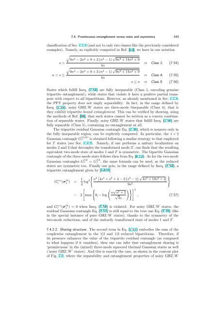
7.4. Promiscuous entanglement versus noise and asymmetry 143
classification of Sec. 7.1.1 (and not to only two classes like the previously considered
examples). Namely, as explicitly computed in Ref. [53], we have in our notation
9n
s >
4 − 2n2 + 9 + 3 (n2 − 1) √ 9n4 + 14n2 + 9
4n
9n
n < s ≤
⇒ Class 1; (7.54)
4 − 2n2 + 9 + 3 (n2 − 1) √ 9n4 + 14n2 + 9
4n
⇒ Class 4; (7.55)
s ≤ n ⇒ Class 5. (7.56)
States which fulfill Ineq. (7.54) are fully inseparable (Class 1, encoding genuine
tripartite entanglement), while states that violate it have a positive partial transpose
with respect to all bipartitions. However, as already mentioned in Sec. 7.1.1,
the PPT property does not imply separability. In fact, in the range defined by
Ineq. (7.55), noisy GHZ/W states are three-mode biseparable (Class 4), that is
they exhibit tripartite bound entanglement. This can be verified by showing, using
the methods of Ref. [94], that such states cannot be written as a convex combination
of separable states. Finally, noisy GHZ/W states that fulfill Ineq. (7.56) are
fully separable (Class 5), containing no entanglement at all.
The tripartite residual Gaussian contangle Eq. (7.36), which is nonzero only in
the fully inseparable region, can be explicitly computed. In particular, the 1 × 2
is obtained following a similar strategy to that employed
Gaussian contangle G i|(jk)
τ
for T states (see Sec. 7.3.2). Namely, if one performs a unitary localization on
modes 2 and 3 that decouples the transformed mode 3 ′ , one finds that the resulting
equivalent two-mode state of modes 1 and 2 ′ is symmetric. The bipartite Gaussian
contangle of the three-mode state follows then from Eq. (6.12). As for the two-mode
Gaussian contangles G 1|2
τ
= G 1|3
τ , the same formula can be used, as the reduced
states are symmetric too. Finally one gets, in the range defined by Ineq. (7.54), a
tripartite entanglement given by [GA16]
G res
τ (σ th
s ) = 1
4 log2
2 n 4s4 + s2 + 4 − 2 s2 − 1 √ 4s4 + 10s2 + 4
9s2
−
n
2 max 0, − log
√ s2 2 + 2
√ ,
3s
(7.57)
and G res
τ (σ th
s ) = 0 when Ineq. (7.54) is violated. For noisy GHZ/W states, the
residual Gaussian contangle Eq. (7.57) is still equal to the true one Eq. (7.35) (like
in the special instance of pure GHZ/W states), thanks to the symmetry of the
two-mode reductions, and of the unitarily transformed state of modes 1 and 2 ′ .
7.4.2.2. Sharing structure. The second term in Eq. (7.57) embodies the sum of the
couplewise entanglement in the 1|2 and 1|3 reduced bipartitions. Therefore, if
its presence enhances the value of the tripartite residual contangle (as compared
to what happens if it vanishes), then one can infer that entanglement sharing is
‘promiscuous’ in the (mixed) three-mode squeezed thermal Gaussian states as well
(‘noisy GHZ/W ’ states). And this is exactly the case, as shown in the contour plot
of Fig. 7.6, where the separability and entanglement properties of noisy GHZ/W