ENTANGLEMENT OF GAUSSIAN STATES Gerardo Adesso

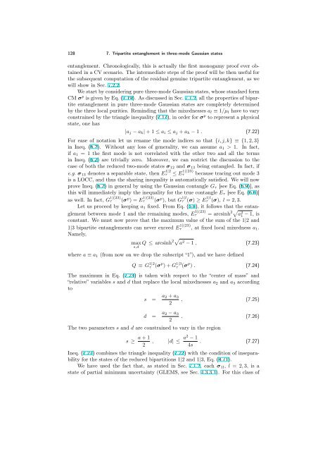
128 7. Tripartite entanglement in three-mode Gaussian states
entanglement. Chronologically, this is actually the first monogamy proof ever obtained
in a CV scenario. The intermediate steps of the proof will be then useful for
the subsequent computation of the residual genuine tripartite entanglement, as we
will show in Sec. 7.2.2.
We start by considering pure three-mode Gaussian states, whose standard form
CM σ p is given by Eq. (7.19). As discussed in Sec. 7.1.2, all the properties of bipartite
entanglement in pure three-mode Gaussian states are completely determined
by the three local purities. Reminding that the mixednesses al ≡ 1/µl have to vary
constrained by the triangle inequality (7.17), in order for σ p to represent a physical
state, one has
|aj − ak| + 1 ≤ ai ≤ aj + ak − 1 . (7.22)
For ease of notation let us rename the mode indices so that {i, j, k} ≡ {1, 2, 3}
in Ineq. (6.2). Without any loss of generality, we can assume a1 > 1. In fact,
if a1 = 1 the first mode is not correlated with the other two and all the terms
in Ineq. (6.2) are trivially zero. Moreover, we can restrict the discussion to the
case of both the reduced two-mode states σ12 and σ13 being entangled. In fact, if
e.g. σ13 denotes a separable state, then E 1|2
τ
≤ E 1|(23)
τ
because tracing out mode 3
is a LOCC, and thus the sharing inequality is automatically satisfied. We will now
prove Ineq. (6.2) in general by using the Gaussian contangle Gτ [see Eq. (6.9)], as
this will immediately imply the inequality for the true contangle Eτ [see Eq. (6.6)]
as well. In fact, G 1|(23)
τ
(σ p ) = E 1|(23)
τ
(σ p ), but G 1|l
τ (σ) ≥ E 1|l
τ (σ), l = 2, 3.
Let us proceed by keeping a1 fixed. From Eq. (6.8), it follows that the entanglement
between mode 1 and the remaining modes, E 1|(23)
τ = arcsinh 2 a2 1 − 1, is
constant. We must now prove that the maximum value of the sum of the 1|2 and
1|3 bipartite entanglements can never exceed E 1|(23)
τ , at fixed local mixedness a1.
Namely,
max
s,d Q ≤ arcsinh2 a 2 − 1 , (7.23)
where a ≡ a1 (from now on we drop the subscript “1”), and we have defined
Q ≡ G 1|2
τ (σ p ) + G 1|3
τ (σ p ) . (7.24)
The maximum in Eq. (7.23) is taken with respect to the “center of mass” and
“relative” variables s and d that replace the local mixednesses a2 and a3 according
to
s = a2 + a3
2
d = a2 − a3
2
, (7.25)
. (7.26)
The two parameters s and d are constrained to vary in the region
s ≥
a + 1
2
, |d| ≤ a2 − 1
4s
. (7.27)
Ineq. (7.27) combines the triangle inequality (7.22) with the condition of inseparability
for the states of the reduced bipartitions 1|2 and 1|3, Eq. (4.71).
We have used the fact that, as stated in Sec. 7.1.2, each σ1l, l = 2, 3, is a
state of partial minimum uncertainty (GLEMS, see Sec. 4.3.3.1). For this class of