ENTANGLEMENT OF GAUSSIAN STATES Gerardo Adesso
ENTANGLEMENT OF GAUSSIAN STATES Gerardo Adesso
ENTANGLEMENT OF GAUSSIAN STATES Gerardo Adesso

Create successful ePaper yourself
Turn your PDF publications into a flip-book with our unique Google optimized e-Paper software.
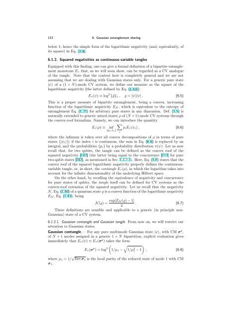
112 6. Gaussian entanglement sharing<br />
below 1; hence the simple form of the logarithmic negativity (and, equivalently, of<br />
its square) in Eq. (6.4).<br />
6.1.2. Squared negativities as continuous-variable tangles<br />
Equipped with this finding, one can give a formal definition of a bipartite entanglement<br />
monotone Eτ that, as we will soon show, can be regarded as a CV analogue<br />
of the tangle. Note that the context here is completely general and we are not<br />
assuming that we are dealing with Gaussian states only. For a generic pure state<br />
|ψ〉 of a (1 + N)-mode CV system, we define our measure as the square of the<br />
logarithmic negativity [the latter defined by Eq. (1.43)]:<br />
Eτ (ψ) ≡ log 2 ˜ϱ1 , ϱ = |ψ〉〈ψ| . (6.5)<br />
This is a proper measure of bipartite entanglement, being a convex, increasing<br />
function of the logarithmic negativity EN , which is equivalent to the entropy of<br />
entanglement Eq. (1.25) for arbitrary pure states in any dimension. Def. (6.5) is<br />
naturally extended to generic mixed states ρ of (N + 1)-mode CV systems through<br />
the convex-roof formalism. Namely, we can introduce the quantity<br />
Eτ (ρ) ≡ inf<br />
{pi,ψi}<br />
<br />
piEτ (ψi) , (6.6)<br />
where the infimum is taken over all convex decompositions of ρ in terms of pure<br />
states {|ψi〉}; if the index i is continuous, the sum in Eq. (6.6) is replaced by an<br />
integral, and the probabilities {pi} by a probability distribution π(ψ). Let us now<br />
recall that, for two qubits, the tangle can be defined as the convex roof of the<br />
squared negativity [142] (the latter being equal to the concurrence [113] for pure<br />
two-qubit states [247], as mentioned in Sec. 1.4.2.1). Here, Eq. (6.6) states that the<br />
convex roof of the squared logarithmic negativity properly defines the continuousvariable<br />
tangle, or, in short, the contangle Eτ (ρ), in which the logarithm takes into<br />
account for the infinite dimensionality of the underlying Hilbert space.<br />
On the other hand, by recalling the equivalence of negativity and concurrence<br />
for pure states of qubits, the tangle itself can be defined for CV systems as the<br />
convex-roof extension of the squared negativity. Let us recall that the negativity<br />
N , Eq. (1.40) of a quantum state ϱ is a convex function of the logarithmic negativity<br />
EN , Eq. (1.43), being<br />
N (ϱ) = exp[EN (ϱ) − 1]<br />
. (6.7)<br />
These definitions are sensible and applicable to a generic (in principle non-<br />
Gaussian) state of a CV system.<br />
6.1.2.1. Gaussian contangle and Gaussian tangle. From now on, we will restrict our<br />
attention to Gaussian states.<br />
Gaussian contangle.— For any pure multimode Gaussian state |ψ〉, with CM σp ,<br />
of N + 1 modes assigned in a generic 1 × N bipartition, explicit evaluation gives<br />
immediately that Eτ (ψ) ≡ Eτ (σp ) takes the form<br />
Eτ (σ p ) = log 2<br />
<br />
1/µ1 − 1/µ 2 <br />
1 − 1 , (6.8)<br />
where µ1 = 1/ √ Det σ1 is the local purity of the reduced state of mode 1 with CM<br />
σ1.<br />
i<br />
2