ENTANGLEMENT OF GAUSSIAN STATES Gerardo Adesso
ENTANGLEMENT OF GAUSSIAN STATES Gerardo Adesso ENTANGLEMENT OF GAUSSIAN STATES Gerardo Adesso
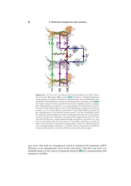
98 5. Multimode entanglement under symmetry 1 2 3 1 2 3 2' 3' Figure 5.1. “If You Cut The Head Of A Basset Hound, It Will Grow Again” (by F. Illuminati, 2001; see also [207], Chapter 1). Graphical depiction of the process of unitary localization (concentration) and delocalization (distribution) of entanglement in three-mode bisymmetric Gaussian states [GA5] (or “basset hound” states), described in the text. Initially, mode 1 is entangled (entanglement is depicted as a waving string) with both modes 2 and 3. It exists a local (with respect to the 1|(23) bipartition) symplectic operation, realized e.g. via a beam-splitter (denoted by a black thick dash), such that all the entanglement is concentrated between mode 1 and the transformed mode 2 ′ , while the other transformed mode 3 ′ decouples from the rest of the system (unitary localization). Therefore, the head of the basset hound (mode 3 ′ ) has been cut off. However, being realized through a symplectic operation (i.e. unitary on the density matrix), the process is reversible: operating on modes 2 ′ and 3 ′ with the inverse symplectic transformation, yields the original modes 2 and 3 entangled again with mode 1, without any loss of quantum correlations (unitary delocalization): the head of the basset hound is back again. once more, that such an entanglement switch is endowed with maximum (100%) efficiency, as no entanglement is lost in the conversions. This fact may have a remarkable impact in the context of quantum repeaters [41] for communications with continuous variables.
5.2. Quantification and scaling of entanglement in fully symmetric states 99 5.1.3.1. The case of the basset hound. To give an example, we can consider a bisymmetric 1 × 2 three-mode Gaussian state, 12 where the CM of the last two modes (constituting subsystem SB) is assumed in standard form, Eq. (2.54). Because of the symmetry, the local symplectic transformation responsible for entanglement concentration in this simple case is the identity on the first mode (constituting subsystem SA) and just a 50:50 beam-splitter transformation B2,3(1/2), Eq. (2.26), on the last two modes [268] (see also Sec. 9.2.1). The entire procedure of unitary localization and delocalization of entanglement [GA5] is depicted in Fig. 5.1. Interestingly, it may be referred to as “cut-off and regrowth of the head of a basset hound”, where in our example the basset hound pictorially represents a bisymmetric three-mode state. However, the breed of the dog reflects the fact that the unitary localizability is a property that extends to all 1×N [GA4] and M ×N [GA5] bisymmetric Gaussian states (in which case, the basset hound’s body would be longer and longer with increasing N). We can therefore address bisymmetric Gaussian states as basset hound states, if desired. In this canine analogy, let us take the freedom to remark that fully symmetric states of the form Eq. (2.60), as a special case, are of course bisymmetric under any bipartition of the modes; this, in brief, means that any conceivable multimode, bipartite entanglement is locally equivalent to the minimal two-mode, bipartite entanglement (consequences of this will be deeply investigated in the following). Pictorially, remaining in the context of three-mode Gaussian states, this special type of basset hound state resembles a Cerberus state, in which any one of the three heads can be cut and can be reversibly regrown. 5.2. Quantification and scaling of entanglement in fully symmetric states In this Section we will explicitly compute the block entanglement (i.e. the entanglement between different blocks of modes) for some instances of multimode Gaussian states. We will study its scaling behavior as a function of the number of modes and explore in deeper detail the localizability of the multimode entanglement. We focus our attention on fully symmetric L-mode Gaussian states (the number of modes is denoted by L in general to avoid confusion), endowed with complete permutation invariance under mode exchange, and described by a 2L × 2L CM σ β L given by Eq. (2.60). These states are trivially bisymmetric under any bipartition of the modes, so that their block entanglement is always localizable by means of local symplectic operations. Let us recall that concerning the covariances in normal forms of fully symmetric states (see Sec. 2.4.3), pure L-mode states are characterized by ν − β = ν+ β L = 1 in Eq. (2.61), which yields z1 = (L − 2)(b2 − 1) + (b 2 − 1) [L ((b 2 − 1) L + 4) − 4] 2b(L − 1) z2 = (L − 2)(b2 − 1) − (b 2 − 1) [L ((b 2 − 1) L + 4) − 4] 2b(L − 1) , . (5.13) 12 The bipartite and genuinely tripartite entanglement structure of three-mode Gaussian states will be extensively investigated in Chapter 7, based on Ref. [GA11]. The bisymmetric three-mode Gaussian states will be also reconsidered as efficient resources for 1 → 2 telecloning of coherent states in Sec. 12.3, based on Ref. [GA16].
- Page 61 and 62: 2.4. Standard forms of Gaussian cov
- Page 63: Part II Bipartite entanglement of G
- Page 66 and 67: 52 3. Characterizing entanglement o
- Page 68 and 69: 54 3. Characterizing entanglement o
- Page 71 and 72: CHAPTER 4 Two-mode entanglement Thi
- Page 73 and 74: 4.2. Entanglement and symplectic ei
- Page 75 and 76: 4.3. Entanglement versus Entropic m
- Page 77 and 78: 1 0.75 0.5 SL1 0.25 0 (a) 4.3. Enta
- Page 79 and 80: 4.3. Entanglement versus Entropic m
- Page 81 and 82: Μ Μ1Μ2 3 2 1 1 4.3. Entanglemen
- Page 83 and 84: 4.3. Entanglement versus Entropic m
- Page 85 and 86: 4.3. Entanglement versus Entropic m
- Page 87 and 88: global generalized entropy S3 globa
- Page 89 and 90: 4.4. Quantifying entanglement via p
- Page 91 and 92: 4.4. Quantifying entanglement via p
- Page 93 and 94: 4.5. Gaussian entanglement measures
- Page 95 and 96: 4.5. Gaussian entanglement measures
- Page 97 and 98: 4.5. Gaussian entanglement measures
- Page 99 and 100: 4.5. Gaussian entanglement measures
- Page 101 and 102: Ν p Σopt 1 0.8 0.6 0.4 0.2 0 4.5
- Page 103 and 104: GEF GEF 4 3 2 1 0 4.6. Summary and
- Page 105: 4.6. Summary and further remarks 91
- Page 108 and 109: 94 5. Multimode entanglement under
- Page 110 and 111: 96 5. Multimode entanglement under
- Page 114 and 115: 100 5. Multimode entanglement under
- Page 116 and 117: 102 5. Multimode entanglement under
- Page 118 and 119: 104 5. Multimode entanglement under
- Page 121: Part III Multipartite entanglement
- Page 124 and 125: 110 6. Gaussian entanglement sharin
- Page 126 and 127: 112 6. Gaussian entanglement sharin
- Page 128 and 129: 114 6. Gaussian entanglement sharin
- Page 130 and 131: 116 6. Gaussian entanglement sharin
- Page 132 and 133: 118 6. Gaussian entanglement sharin
- Page 134 and 135: 120 6. Gaussian entanglement sharin
- Page 136 and 137: 122 7. Tripartite entanglement in t
- Page 138 and 139: 124 7. Tripartite entanglement in t
- Page 140 and 141: 126 7. Tripartite entanglement in t
- Page 142 and 143: 128 7. Tripartite entanglement in t
- Page 144 and 145: 130 7. Tripartite entanglement in t
- Page 146 and 147: 132 7. Tripartite entanglement in t
- Page 148 and 149: 134 7. Tripartite entanglement in t
- Page 150 and 151: 136 7. Tripartite entanglement in t
- Page 152 and 153: 138 7. Tripartite entanglement in t
- Page 154 and 155: 140 7. Tripartite entanglement in t
- Page 156 and 157: 142 7. Tripartite entanglement in t
- Page 158 and 159: 144 7. Tripartite entanglement in t
- Page 160 and 161: 146 7. Tripartite entanglement in t
98 5. Multimode entanglement under symmetry<br />
1 2 3<br />
1 2 3<br />
2' 3'<br />
Figure 5.1. “If You Cut The Head Of A Basset Hound, It Will Grow<br />
Again” (by F. Illuminati, 2001; see also [207], Chapter 1). Graphical depiction<br />
of the process of unitary localization (concentration) and delocalization (distribution)<br />
of entanglement in three-mode bisymmetric Gaussian states [GA5]<br />
(or “basset hound” states), described in the text. Initially, mode 1 is entangled<br />
(entanglement is depicted as a waving string) with both modes 2 and 3.<br />
It exists a local (with respect to the 1|(23) bipartition) symplectic operation,<br />
realized e.g. via a beam-splitter (denoted by a black thick dash), such that all<br />
the entanglement is concentrated between mode 1 and the transformed mode<br />
2 ′ , while the other transformed mode 3 ′ decouples from the rest of the system<br />
(unitary localization). Therefore, the head of the basset hound (mode 3 ′ ) has<br />
been cut off. However, being realized through a symplectic operation (i.e. unitary<br />
on the density matrix), the process is reversible: operating on modes 2 ′<br />
and 3 ′ with the inverse symplectic transformation, yields the original modes 2<br />
and 3 entangled again with mode 1, without any loss of quantum correlations<br />
(unitary delocalization): the head of the basset hound is back again.<br />
once more, that such an entanglement switch is endowed with maximum (100%)<br />
efficiency, as no entanglement is lost in the conversions. This fact may have a remarkable<br />
impact in the context of quantum repeaters [41] for communications with<br />
continuous variables.


