ENTANGLEMENT OF GAUSSIAN STATES Gerardo Adesso

Ν p
Σopt 1
0.8
0.6
0.4
0.2
0
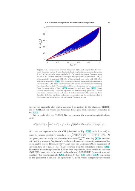
4.5. Gaussian entanglement measures versus Negativities 87
0 0.2 0.4 0.6 0.8 1
Ν Σ
Figure 4.9. Comparison between Gaussian EMs and negativities for twomode
Gaussian states. On the horizontal axis we plot the symplectic eigenvalue
˜ν−(σ) of the partially transposed CM ˜σ of a generic two-mode Gaussian state
with CM σ. On the vertical axis we plot the symplectic eigenvalue ˜ν−(σ p
opt )
of the partially transposed CM ˜σ p
opt
of the optimal pure state with CM σp
opt ,
which minimizes Eq. (3.11). The negativities are all monotonically decreasing
functions of ˜ν−(σ), while the Gaussian EMs are all monotonically decreasing
functions of ˜ν−(σ p
opt ). The equation of the two boundary curves are obtained
from the saturation of Ineq. (4.78) (upper bound) and Ineq. (4.81) (lower
bound), respectively. The dots represent 50 000 randomly generated CMs of
two-mode Gaussian states. Of up to 1 million random CMs, none has been
found to lie below the lower solid-line curve, enforcing the conjecture that it
be an absolute boundary for all two-mode Gaussian states.
But we can promptly give partial answers if we restrict to the classes of GLEMS
and of GMEMS, for which the Gaussian EMs have been explicitly computed in
Sec. 4.5.2.
Let us begin with the GLEMS. We can compute the squared symplectic eigenvalue
˜ν 2 −(σ GLEMS ) =
4(s 2 + d 2 ) − g 2
− 1 − (4(s2 + d2 ) − g2 − 1) 2 − 4g2
/2 .
Next, we can reparametrize the CM (obtained
by Eq. (4.68) with λ = −1) to
make ˜ν− appear explicitly, namely g = ˜ν 2 −[4(s2 + d2 ) − 1 − ˜ν 2 −]/(1 + ˜ν 2 −). At
this point, one can study the piecewise function m2GLEMS opt from Eq. (4.74), and find
out that it is a convex function of d in the whole space of parameters corresponding
to entangled states. Hence, m2GLEMS opt , and thus the Gaussian EM, is maximized at
the boundary |d| = (2˜ν−s − ˜ν 2 − − 1)/2, resulting from the saturation of Ineq. (4.69).
The states maximizing Gaussian EMs at fixed negativities, if we restrict to the class
of GLEMS, have then to be found in the subclass of GMEMMS (states of maximal
negativity for fixed marginals [GA3], defined by Eq. (4.1) in Sec. 4.3.2), depending
on the parameter s and on the eigenvalue ˜ν− itself, which completely determines