Recovery Plan for the Mexican Spotted Owl (Strix occidentalis lucida )
Recovery Plan for the Mexican Spotted Owl (Strix occidentalis lucida )
Recovery Plan for the Mexican Spotted Owl (Strix occidentalis lucida )

Create successful ePaper yourself
Turn your PDF publications into a flip-book with our unique Google optimized e-Paper software.
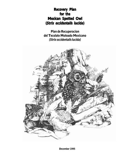
<strong>Recovery</strong> <strong>Recovery</strong> <strong>Plan</strong><br />
<strong>Plan</strong><br />
<strong>for</strong> <strong>for</strong> <strong>the</strong><br />
<strong>the</strong><br />
<strong>Mexican</strong> <strong>Mexican</strong> <strong>Spotted</strong> <strong>Spotted</strong> <strong>Owl</strong><br />
<strong>Owl</strong><br />
(<strong>Strix</strong> <strong>Strix</strong> <strong>occidentalis</strong> <strong>occidentalis</strong> <strong>lucida</strong> <strong>lucida</strong>) <strong>lucida</strong><br />
<strong>Plan</strong> de Recuperacion<br />
del Tecolate Moteado <strong>Mexican</strong>o<br />
(<strong>Strix</strong> <strong>occidentalis</strong> <strong>lucida</strong>)<br />
December 1995
Primary Primary Primary Authors:<br />
Authors:<br />
<strong>Recovery</strong> <strong>Recovery</strong> <strong>Plan</strong><br />
<strong>Plan</strong><br />
<strong>for</strong> <strong>for</strong> <strong>the</strong><br />
<strong>the</strong><br />
<strong>Mexican</strong> <strong>Mexican</strong> <strong>Mexican</strong> <strong>Spotted</strong> <strong>Spotted</strong> <strong>Owl</strong><br />
<strong>Owl</strong><br />
(<strong>Strix</strong> <strong>Strix</strong> <strong>occidentalis</strong> <strong>occidentalis</strong> <strong>lucida</strong> <strong>lucida</strong>) <strong>lucida</strong><br />
<strong>Plan</strong> de Recuperacion<br />
del Tecolate Moteado <strong>Mexican</strong>o<br />
(<strong>Strix</strong> <strong>occidentalis</strong> <strong>lucida</strong>)<br />
Nancy M. Kaufman, Regional Director,<br />
U.S. Department of <strong>the</strong> Interior, Fish and Wildlife Service,<br />
Southwestern Region<br />
William M. Block; Fernando Clemente; Jack F. Cully; James L. Dick, Jr.; Alan B. Franklin;<br />
Joseph L. Ganey; Frank P. Howe; W.H. Moir; Steven L. Spangle; Sarah E. Rinkevich; Dean L. Urban;<br />
Robert Vahle; James P. Ward, Jr.; and Gary C. White<br />
O<strong>the</strong>r O<strong>the</strong>r Contributors:<br />
Contributors:<br />
Kevin J. Cook (Technical Editor): Brian Geils (Disturbance Analyses);<br />
Kate W. Grandison (Meeting Facilitator); Tim Keitt (Landscape Analyses); Juan F. Martinez-Montoya<br />
(<strong>Mexican</strong> <strong>Recovery</strong> Units); Art Needleman and Jill Simmons (Layout and Design);<br />
Joyce V. Patterson (Illustrator); Tom Spalding (State of Arizona); Rich Teck (Forest Modeling);<br />
Steven Thompson (Southwestern Tribal Liaison); Brenda E. Witsell (Administrative Assistant).<br />
1995<br />
Approved:__________________________________________________ Date:_____________<br />
Regional Director, U.S. Fish and Wildlife Service
DISCLAIMER:<br />
DISCLAIMER:<br />
This <strong>Recovery</strong> <strong>Plan</strong> is not intended to provide details on all aspects of <strong>Mexican</strong> spotted owl management.<br />
The <strong>Recovery</strong> <strong>Plan</strong> outlines steps necessary to bring about recovery of <strong>the</strong> species. The <strong>Recovery</strong> <strong>Plan</strong> is not<br />
a “decision document” as defined by <strong>the</strong> National Environmental Policy Act (NEPA). It does not allocate<br />
resources on public lands. The implementation of <strong>the</strong> recovery plan is <strong>the</strong> responsibility of Federal and State<br />
management agencies in areas where <strong>the</strong> species occurs. Implementation is done through incorporation of<br />
appropriate portions of <strong>the</strong> <strong>Recovery</strong> <strong>Plan</strong> in agency decision documents such as <strong>for</strong>est plans, park management<br />
plans, and State game management plans. Such documents are <strong>the</strong>n subject to <strong>the</strong> NEPA process <strong>for</strong><br />
public review and selection of alternatives.<br />
LITERATURE LITERATURE CITATIONS:<br />
CITATIONS:<br />
This document should be referenced in literature citations as follows:<br />
USDI Fish and Wildlife Service. 1995. <strong>Recovery</strong> plan <strong>for</strong> <strong>the</strong> <strong>Mexican</strong> spotted owl: Vol.I.<br />
Albuquerque, New Mexico. XXXpp.<br />
A fee <strong>for</strong> additional copies of this document will be charged depending on <strong>the</strong> number of pages<br />
and postage. Additional copies of this document may be purchased from:<br />
Fish and Wildlife Reference Service<br />
5430 Grosvenor Lane, Suite 110<br />
Be<strong>the</strong>sda, MD 20814<br />
(303) 492-6403<br />
1-800-582-3421
<strong>Mexican</strong> <strong>Spotted</strong> <strong>Owl</strong> <strong>Recovery</strong> <strong>Plan</strong><br />
MEXICAN MEXICAN SPO SPOTTED SPO TED O OOWL<br />
O WL RECO RECOVER RECO VER VERY VER Y PL PLAN PL AN<br />
Table Table of of Contents<br />
Contents<br />
List List of of Tables ables ables ................................................................................................................................ ................................................................................................................................ vii<br />
vii<br />
List List of of F FFigur<br />
F igur igures igur es ............................................................................................................................... ............................................................................................................................... viii<br />
viii<br />
Executiv ecutiv ecutive ecutiv e S SSummar<br />
S ummar ummary ummar ....................................................................................................................... ....................................................................................................................... ix<br />
ix<br />
Ackno ckno cknowledgments<br />
ckno wledgments wledgments........................................................................................................................<br />
wledgments ........................................................................................................................ xiii<br />
xiii<br />
PAR AR ART AR T I: I: PL PLAN PL AN DE DEVEL DE VEL VELOPMENT<br />
VEL OPMENT<br />
A. A. RECO RECOVER RECO RECO VER VERY VERY<br />
Y PL PLANNING<br />
PL ANNING ................................................................................................ ................................................................................................ 1<br />
B. B. LISTING LISTING ............................................................................................................................ ............................................................................................................................ 2<br />
The Present or Threatened Destruction, Modificiation, or Curtailment<br />
of its Habitat or Range .....................................................................................................2<br />
Overutilization <strong>for</strong> Commercial, Recreational, Scientific, or Educational<br />
Purposes ..........................................................................................................................3<br />
Disease or Predation ........................................................................................................ 3<br />
Inadequacy of Existing Regulatory Mechanisms ...................................................................3<br />
O<strong>the</strong>r Natural or Manmade Factors Affecting Its Continued Existence ................................3<br />
C. C. PP<br />
PAST PP<br />
AST AND AND CURRENT CURRENT MANA MANAGEMENT MANA GEMENT OF OF THE<br />
THE<br />
MEXICAN MEXICAN SPO SPOTTED SPO TED O OOWL<br />
O OWL<br />
WL .......................................................................................... .......................................................................................... 4<br />
Fish and Wildlife Service ...................................................................................................... 4<br />
Forest Service ....................................................................................................................... 4<br />
Forest Service Southwestern Region (Region 3) ................................................................ 4<br />
Forest Service Rocky Mountain Region (Region 2) .......................................................... 5<br />
Forest Service Intermountain Region (Region 4) .............................................................. 5<br />
O<strong>the</strong>r Federal Agencies ........................................................................................................ 6<br />
National Park Service ....................................................................................................... 6<br />
Bureau of Land Management ........................................................................................... 6<br />
Department of Defense ................................................................................................... 6<br />
States ................................................................................................................................... 7<br />
Arizona............................................................................................................................ 7<br />
New Mexico .................................................................................................................... 7<br />
Colorado ......................................................................................................................... 7<br />
Utah ................................................................................................................................ 7<br />
Texas ............................................................................................................................... 8<br />
Tribes .................................................................................................................................. 8<br />
Mescalero Apache Tribe ................................................................................................... 8<br />
White Mountain Apache Tribe......................................................................................... 8<br />
San Carlos Apache Tribe .................................................................................................. 9<br />
Jicarilla Apache ................................................................................................................ 9<br />
Navajo Nation ................................................................................................................. 9<br />
Mexico ................................................................................................................................ 9<br />
D. D. CONSIDERA<br />
CONSIDERA<br />
CONSIDERATIONS CONSIDERA<br />
CONSIDERATIONS<br />
TIONS IN IN PL PLAN PL AN DE DEVEL DE DEVEL<br />
VEL VELOPMENT<br />
VEL OPMENT ....................................................... ....................................................... 11<br />
11<br />
<strong>Recovery</strong> Units .................................................................................................................... 11<br />
The Current Situation ......................................................................................................... 11<br />
<strong>Recovery</strong> <strong>Plan</strong> Duration ....................................................................................................... 12<br />
Conservation <strong>Plan</strong>s <strong>for</strong> O<strong>the</strong>r <strong>Spotted</strong> <strong>Owl</strong> Subspecies ......................................................... 13<br />
i
<strong>Mexican</strong> <strong>Spotted</strong> <strong>Owl</strong> <strong>Recovery</strong> <strong>Plan</strong><br />
Ecosystem Management ..................................................................................................... 15<br />
Economic Considerations ...................................................................................................16<br />
Human Intervention and Natural Processes ........................................................................17<br />
Differences Between <strong>the</strong> Draft and Final <strong>Recovery</strong> <strong>Plan</strong>s .....................................................17<br />
PAR AR ART AR T II: II: BIOL BIOLOGICAL BIOL OGICAL AND AND AND ECOL ECOLOGICAL ECOL OGICAL BA BACK BA CK CKGR CK GR GROUND GR OUND<br />
A. A. GENERAL GENERAL BIOL BIOLOGY BIOL OGY AND AND AND ECOL ECOLOGICAL ECOL OGICAL REL RELATIONSHIPS<br />
REL TIONSHIPS<br />
OF OF THE THE MEXICAN MEXICAN SPO SPOTTED SPO TED O OOWL<br />
O WL ......................................................................... ......................................................................... 19<br />
19<br />
Taxonomy ..........................................................................................................................19<br />
Description ........................................................................................................................21<br />
Distribution and Abundance ..............................................................................................21<br />
Habitat Associations ........................................................................................................... 26<br />
Nesting and Roosting Habitat.........................................................................................26<br />
Foraging Habitat ............................................................................................................27<br />
Territoriality and Home Range ...........................................................................................27<br />
Vocalizations ......................................................................................................................28<br />
Interspecific Competition ...................................................................................................28<br />
Feeding Habitats and Prey Ecology .....................................................................................28<br />
Reproductive Biology .........................................................................................................29<br />
Mortality Factors ................................................................................................................31<br />
Predation ........................................................................................................................31<br />
Starvation .......................................................................................................................31<br />
Accidents ........................................................................................................................31<br />
Disease and Parasites .......................................................................................................32<br />
Population Biology ............................................................................................................. 32<br />
Survival ..........................................................................................................................32<br />
Reproduction .................................................................................................................33<br />
Environmental Variation.................................................................................................33<br />
Population Trends ...........................................................................................................33<br />
Movements.........................................................................................................................33<br />
Seasonal Movements. ...................................................................................................... 33<br />
Natal Dispersal ...............................................................................................................33<br />
Landscape Pattern and Metapopulation Structure ...............................................................34<br />
Conclusions .......................................................................................................................34<br />
B. B. RECO RECOVER RECO VER VERY VER Y UNIT UNITS........................................................................................................<br />
UNIT UNIT ........................................................................................................ 36<br />
36<br />
United States ......................................................................................................................36<br />
Colorado Plateau ............................................................................................................36<br />
Sou<strong>the</strong>rn Rocky Mountains - Colorado...........................................................................40<br />
Sou<strong>the</strong>rn Rocky Mountains - New Mexico......................................................................40<br />
Upper Gila Mountains....................................................................................................44<br />
Basin and Range - West ..................................................................................................46<br />
Basin and Range - East ...................................................................................................46<br />
Mexico ...............................................................................................................................49<br />
Sierra Madre Occidental - Norte .....................................................................................49<br />
Sierra Madre Oriental- Norte .......................................................................................... 50<br />
Sierra Madre Occidental - Sur........................ .................................................................50<br />
Sierra Madre Oriental - Sur.............................................................................................51<br />
Eje Neovolcanico ............................................................................................................51<br />
ii
<strong>Mexican</strong> <strong>Spotted</strong> <strong>Owl</strong> <strong>Recovery</strong> <strong>Plan</strong><br />
C. C. DEFINITIONS DEFINITIONS OF OF FOREST FOREST CO COVER CO VER TYP YP YPES YP ES ES.............................................................<br />
ES ............................................................. 52<br />
52<br />
Literature Review................................................................................................................52<br />
Ponderosa Pine ...............................................................................................................53<br />
Mixed-conifer .................................................................................................................53<br />
Spruce-fir .......................................................................................................................54<br />
O<strong>the</strong>r Forest Types of Interest .........................................................................................54<br />
Chihuahua Pine..........................................................................................................54<br />
Quaking Aspen ...........................................................................................................55<br />
Riparian Forests ..........................................................................................................55<br />
<strong>Plan</strong> Definitions .................................................................................................................55<br />
Ponderosa Pine Forest .....................................................................................................55<br />
Pine-oak Forest ...............................................................................................................55<br />
Mixed-conifer Forest.......................................................................................................56<br />
High-elevation Forests, Including Spruce-fir Forest .........................................................57<br />
Quaking Aspen...............................................................................................................57<br />
Key to Forest Types.............................................................................................................57<br />
D. D. CONCEPTU<br />
CONCEPTUAL CONCEPTU AL FRAME FRAMEWORK FRAME ORK FOR FOR RECO RECOVER RECO VER VERY....................................................<br />
VER .................................................... 59<br />
59<br />
Ecosystem or Landscape Management ................................................................................59<br />
Fire.................................................................................................................................60<br />
O<strong>the</strong>r Natural Disturbances ............................................................................................61<br />
Degradation of Riparian Forests ......................................................................................65<br />
Timber Harvest and Silvicultural Practices ..........................................................................65<br />
Historical Perspectives ....................................................................................................65<br />
Past Practices ..............................................................................................................65<br />
Forest <strong>Plan</strong>s ................................................................................................................66<br />
Habitat Trends ............................................................................................................66<br />
Data Availability .....................................................................................................66<br />
Trends in Forest Land Base and Timber Volume ...................................................... 67<br />
Trends in Forest Types ............................................................................................67<br />
Trends in Size-class Distibutions .............................................................................68<br />
Summary of Recent Habitat Trends ........................................................................68<br />
Silvicultural Practices and Forest Management ................................................................68<br />
Silviculture .................................................................................................................69<br />
Even-aged Management .......................................................................................... 69<br />
Uneven-aged Management......................................................................................70<br />
Development and Maintenance of Stratified Mixtures .............................................71<br />
Conclusions.................................................................................................................... 71<br />
Grazing .............................................................................................................................. 72<br />
Recreation .......................................................................................................................... 73<br />
Types of Recreation ........................................................................................................ 73<br />
Camping .................................................................................................................... 74<br />
Hiking ....................................................................................................................... 74<br />
Off-road Vehicles ....................................................................................................... 74<br />
Rock Climbing ........................................................................................................ . 74<br />
Wildlife Viewing and Photography........................................................................... . 74<br />
Recreation Summary .................................................................................................. .74<br />
Summary........................................................................................................................... .75<br />
iii
PAR AR ART AR T III: III: RECO RECOVER RECO VER VERY VER<br />
<strong>Mexican</strong> <strong>Spotted</strong> <strong>Owl</strong> <strong>Recovery</strong> <strong>Plan</strong><br />
A. A. DELISTING DELISTING .................................................................................................................... .................................................................................................................... 76 76<br />
76<br />
The Delisting Process ........................................................................................................ 76<br />
Delisting Criteria ............................................................................................................... 76<br />
Monitoring Population Trends ....................................................................................... 77<br />
O<strong>the</strong>r Considerations of Population Monitoring ........................................................ 79<br />
Monitoring Habitat Trends ............................................................................................ 79<br />
Long-term Management <strong>Plan</strong> ........................................................................................ 80<br />
Delisting at <strong>the</strong> <strong>Recovery</strong> Unit Level .............................................................................. 80<br />
Moderating and Regulating Threats. .......................................................................... 81<br />
Habitat Trends Within <strong>Recovery</strong> Units ....................................................................... 81<br />
B. B. GENERAL GENERAL APPR APPROACH<br />
APPR CH ................................................................................................ ................................................................................................ 82<br />
82<br />
Assumptions and Guiding Principles.................................................................................. 82<br />
Assumptions. ................................................................................................................. 83<br />
Guiding Principles ......................................................................................................... 84<br />
General Recommendations ................................................................................................ 84<br />
Protected Areas .............................................................................................................. 84<br />
Protected Activity Center (PAC) ................................................................................ 84<br />
Guidelines ............................................................................................................. 84<br />
Rationale ............................................................................................................... 89<br />
Steep Slopes (Outside of PACs) .................................................................................. 89<br />
Guidelines ............................................................................................................. 89<br />
Rationale ............................................................................................................... 89<br />
Reserved Lands .......................................................................................................... 90<br />
Guidelines ............................................................................................................. 90<br />
Rationale ............................................................................................................... 90<br />
Restricted Areas ............................................................................................................. 90<br />
Existing Conditions ................................................................................................... 91<br />
Reference Conditions ................................................................................................. 91<br />
Nesting and Roosting target/threshold conditions .................................................. 91<br />
Coarse Filter .............................................................................................................. 93<br />
Fine Filter .................................................................................................................. 94<br />
Overriding Guidelines ........................................................................................... 94<br />
Specific Guidelines ................................................................................................ 94<br />
Rationale ............................................................................................................... 95<br />
Riparian Communities............................................................................................... 95<br />
Guidelines ............................................................................................................. 95<br />
Rationale ............................................................................................................... 95<br />
O<strong>the</strong>r Forest and Woodland Types ................................................................................. 95<br />
Grazing Recommendations ................................................................................................ 96<br />
Grazing Guidelines ........................................................................................................ 96<br />
Rationale <strong>for</strong> Grazing Guidelines ................................................................................... 97<br />
Recreation Recommendations............................................................................................ 98<br />
Guidelines ..................................................................................................................... 98<br />
<strong>Recovery</strong> Unit Considerations ........................................................................................... 98<br />
Colorado Plateau ........................................................................................................... 98<br />
Potential Threats ........................................................................................................ 99<br />
Sou<strong>the</strong>rn Rocky Mountains - Colorado.......................................................................... 99<br />
iv
<strong>Mexican</strong> <strong>Spotted</strong> <strong>Owl</strong> <strong>Recovery</strong> <strong>Plan</strong><br />
Potential Threats ........................................................................................................ 99<br />
Sou<strong>the</strong>rn Rocky Mountains - New Mexico..................................................................... 99<br />
Potential Threats ....................................................................................................... 100<br />
Upper Gila Mountains.................................................................................................. 100<br />
Potential Threats ....................................................................................................... 100<br />
Basin and Range - West ................................................................................................ 101<br />
Potential Threats ....................................................................................................... 101<br />
Basin and Range - East ................................................................................................. 102<br />
Potential Threats ....................................................................................................... 102<br />
Mexico ......................................................................................................................... 103<br />
Potential Threats ....................................................................................................... 104<br />
Sierra Madre Occidental - Norte ........................................................................... 104<br />
Sierra Madre Oriental - Norte............................................................................... 104<br />
Sierra Madre Occidental - Sur............................................................................... 104<br />
Sierra Madre Oriental - Sur .................................................................................. 104<br />
Eje Neovolcanico .................................................................................................. 104<br />
C. C. MONIT MONITORING MONIT ORING PR PROCEDURES<br />
PR OCEDURES<br />
OCEDURES.................................................................................<br />
OCEDURES ................................................................................. 105<br />
105<br />
Habitat Monitoring .......................................................................................................... 105<br />
Macrohabitat ................................................................................................................ 105<br />
Microhabitat ................................................................................................................ 106<br />
Population Monitoring ..................................................................................................... 107<br />
Target Population ......................................................................................................... 107<br />
Sampling Units............................................................................................................. 107<br />
Sampling Procedures..................................................................................................... 108<br />
Stratification ............................................................................................................. 108<br />
Selection of Quadrats ................................................................................................ 108<br />
Sampling Within Quadrats ....................................................................................... 108<br />
Banding Birds ........................................................................................................... 109<br />
Statistical Analysis......................................................................................................... 109<br />
Estimation of Capture Probability ............................................................................. 109<br />
Estimation of Density Per Quadrat............................................................................ 110<br />
Estimation of Density Per Stratum ............................................................................ 110<br />
Variance Estimators ................................................................................................... 111<br />
Cormack-Jolly-Seber Models ..................................................................................... 111<br />
Personnel ...................................................................................................................... 111<br />
Training .................................................................................................................... 112<br />
Computerized Data Entry and Summarization.............................................................. 112<br />
Costs ............................................................................................................................ 113<br />
Potential Experiments ................................................................................................... 113<br />
Alternative Designs <strong>for</strong> Population Monitoring ............................................................. 114<br />
Drawing New Samples of Quadrats Each Year ........................................................... 114<br />
Conducting Surveys Less Often than Yearly ............................................................... 115<br />
Adaptive Sampling .................................................................................................... 115<br />
Conclusions ..................................................................................................................... 115<br />
D. D. A AACTIVIT<br />
A ACTIVIT<br />
CTIVIT CTIVITY-SP<br />
CTIVIT -SP -SPECIFIC -SPECIFIC<br />
ECIFIC RESEAR RESEARCH<br />
RESEAR CH ............................................................................ ............................................................................ 116<br />
116<br />
Role of <strong>the</strong> Scientific Process ............................................................................................ 116<br />
Important Ascpects of Experimental Design...................................................................... 117<br />
Limitations in Past Research on <strong>the</strong> <strong>Mexican</strong> <strong>Spotted</strong> <strong>Owl</strong> ................................................ 118<br />
Research Needs................................................................................................................. 118<br />
Dispersal ...................................................................................................................... 119<br />
v
<strong>Mexican</strong> <strong>Spotted</strong> <strong>Owl</strong> <strong>Recovery</strong> <strong>Plan</strong><br />
Genetics. .......................................................................................................................... 120<br />
Habitat ............................................................................................................................. 120<br />
Population Biology ...........................................................................................................120<br />
Threats to <strong>Recovery</strong> .......................................................................................................... 120<br />
O<strong>the</strong>r Ecosystem Components ......................................................................................... 120<br />
E. E. SUMMAR SUMMARY SUMMAR SUMMAR Y OF OF RECO RECOVER RECO VER VERY VER ........................................................................................ ........................................................................................ 121<br />
121<br />
PAR AR ART AR T IV IV: IV : RECO RECOVER RECO RECO VER VERY VER Y PL PLAN PL AN IMPLEMENT<br />
IMPLEMENTATION<br />
IMPLEMENT TION TION<br />
A. A. IMPLEMENTING IMPLEMENTING L LLAWS,<br />
L WS, REGUL REGULATIONS, REGUL TIONS, AND AND A AAUTHORITIES<br />
A UTHORITIES ......................<br />
...................... ...................... 124<br />
124<br />
Endangered Species Act .................................................................................................... 124<br />
Section 4 ...................................................................................................................... 124<br />
Section 5 ...................................................................................................................... 125<br />
Section 6 ...................................................................................................................... 125<br />
Section 7 ...................................................................................................................... 125<br />
Section 8 ...................................................................................................................... 126<br />
Section 9 ...................................................................................................................... 126<br />
Section 10 .................................................................................................................... 126<br />
National Forest Management Act...................................................................................... 126<br />
National Environmental Policy Act ...................................................................................128<br />
Migratory Bird Treaty Act ................................................................................................. 128<br />
Tribal Lands ..................................................................................................................... 128<br />
State and Private Lands ..................................................................................................... 128<br />
Mexico ............................................................................................................................. 128<br />
B. B. IMPLEMENT<br />
IMPLEMENTATION IMPLEMENT<br />
IMPLEMENT TION O OOVERSIGHT<br />
O VERSIGHT ........................................................................... ........................................................................... 129<br />
129<br />
<strong>Recovery</strong> Unit Working Teams.......................................................................................... 129<br />
Continuing Duties of <strong>the</strong> <strong>Recovery</strong> Team ......................................................................... 120<br />
Centralized <strong>Spotted</strong> <strong>Owl</strong> In<strong>for</strong>mation Repository ............................................................. 130<br />
C. C. STEPDO STEPDOWN STEPDO STEPDO WN OUTLINE OUTLINE .............................................................................................. .............................................................................................. 131<br />
131<br />
D. D. D. IMPLEMENT<br />
IMPLEMENT<br />
IMPLEMENTATION IMPLEMENT TION AND AND COST COST SCHEDULE SCHEDULE ....................................................... ....................................................... 137<br />
137<br />
GL GLOSSAR GL OSSAR OSSARY OSSAR ..................................................................................................................... ..................................................................................................................... 145<br />
145<br />
LITERA LITERATURE LITERA TURE CITED CITED ................................................................................................... ................................................................................................... 152<br />
152<br />
APP APPENDIX APP ENDIX A: A: The The The R RReco<br />
R eco ecover eco er ery er y Team eam and and and Associates Associates ....................................................... ....................................................... 163 163<br />
163<br />
APP APPENDIX APP APPENDIX<br />
ENDIX B: B: Schedule Schedule of of MM<br />
Meetings MM<br />
eetings ............................................................................. ............................................................................. 165 165<br />
165<br />
APP APPENDIX APP ENDIX C: C: Schedule Schedule of of F FField<br />
F ield Visits Visits ......................................................................... ......................................................................... 166<br />
166<br />
APP APPENDIX APP ENDIX D: D: List List of of EE<br />
English E nglish and and Latin Latin N NNames<br />
N ames .......................................................... .......................................................... 167<br />
167<br />
APP APPENDIX APP ENDIX E: E: Agencies Agencies Agencies and and P PPersons<br />
P ersons Commenting Commenting on on D DDraft<br />
D raft R RReco<br />
RR<br />
eco ecover eco er ery ery<br />
y P P<strong>Plan</strong><br />
PP<br />
lan ............... ............... 170 170<br />
170<br />
vi
List List of of Tables<br />
Tables<br />
<strong>Mexican</strong> <strong>Spotted</strong> <strong>Owl</strong> <strong>Recovery</strong> <strong>Plan</strong><br />
Table able ES.1 ES.1 Overview of management categories by vegetation type <strong>for</strong> lands not<br />
administratively reserved.................................................................................................................xi<br />
Table able I.D.1 I.D.1 Summary of relative <strong>Mexican</strong> spotted owl population size, timber harvest threat, and fire<br />
threat by <strong>Recovery</strong> Unit.................................................................................................................. 12<br />
Table able II.A.1. II.A.1. Historical records and minimum numbers of <strong>Mexican</strong> spotted owls<br />
found during planned surveys and incidental observations, reported by <strong>Recovery</strong> Unit<br />
and land ownership .................................................................................................................. 23-24<br />
Table able II.B.1. II.B.1. Land-ownership patterns (thousands of hectares) in <strong>Recovery</strong> Units<br />
within <strong>the</strong> United States .................................................................................................................41<br />
Table able II.B.2. II.B.2. Land-ownership patterns (thousands of hectares) in <strong>Recovery</strong> Units<br />
within Mexico ................................................................................................................................50<br />
Table able able II.D.1. II.D.1. Changes in <strong>the</strong> area (ha x 1,000 [ac x 1,000]) and distribution of<br />
<strong>for</strong>est types from <strong>the</strong> 1960s to 1980s on commercial <strong>for</strong>est lands within Arizona<br />
and New Mexico ............................................................................................................................67<br />
Table able II.D.2. II.D.2. Changes in <strong>the</strong> density (trees/ha [trees/ac]) and distribution of<br />
tree size classes from <strong>the</strong> 1960s to 1980s on commercial <strong>for</strong>est lands within Arizona<br />
and New Mexico ............................................................................................................................68<br />
Table able III.B.1 III.B.1 III.B.1 Target/threshold conditions <strong>for</strong> mixed-conifer and pine-oak <strong>for</strong>ests<br />
within restricted areas .....................................................................................................................92<br />
Table able IV IV.1 IV .1 Implementation and cost schedule ..................................................................... 139-144<br />
vii
List List List of of Figures<br />
Figures<br />
<strong>Mexican</strong> <strong>Spotted</strong> <strong>Owl</strong> <strong>Recovery</strong> <strong>Plan</strong><br />
Figur igur igure igur e II.A.1. II.A.1. Geographic range of <strong>the</strong> spotted owl ......................................................................20<br />
Figur igur igure igur e II.A.2. II.A.2. II.A.2. Current distribution of <strong>Mexican</strong> spotted owls in <strong>the</strong> United States<br />
based on planned surveys and incidental observations recorded from 1990 through 1993...............22<br />
Figur igur igure igur e II.A.3. II.A.3. Current distribution of <strong>Mexican</strong> spotted owls in Mexico based on<br />
planned surveys and incidental observations recorded from 1990 through 1993 .............................. 25<br />
Figur igur igure igur e II.A.4. II.A.4. Geographic variability in <strong>the</strong> food habits of <strong>Mexican</strong> spotted owls<br />
represented as relative frequencies of (a) (a) woodrats, (b) (b) voles, (c) (c) gophers, (d) (d) birds,<br />
(e) (e) bats, and (f (f) (f ) reptiles..................................................................................................................30<br />
Figur igur igure igur e II.B.1. II.B.1. II.B.1. <strong>Recovery</strong> Units within <strong>the</strong> United States.................................................................37<br />
Figur igur igure igur e II.B.2. II.B.2. <strong>Recovery</strong> Units within <strong>the</strong> Republic of Mexico ........................................................38<br />
Figur igur igure igur e II.B.3 II.B.3 Colorado Plateau <strong>Recovery</strong> Unit.............................................................................. 39<br />
Figur igur igur igure igur e II.B.4 II.B.4 Sou<strong>the</strong>rn Rocky Mountains - Colorado <strong>Recovery</strong> Unit ............................................42<br />
Figur igur igure igure<br />
e II.B.5 II.B.5 Sou<strong>the</strong>rn Rocky Mountains - New Mexico <strong>Recovery</strong> Unit .......................................43<br />
Figur igur igure igur e II.B.6 II.B.6 Upper Gila Mountains <strong>Recovery</strong> Unit .....................................................................45<br />
Figur igur igure igur e II.B.7 II.B.7 Basin and Range - West <strong>Recovery</strong> Unit ....................................................................47<br />
Figur igur igure igur e II.B.8 II.B.8 Basin and Range - East <strong>Recovery</strong> Unit .....................................................................48<br />
Figur igur igure igur e II.D.1 II.D.1 Historical record of number of total fires and number of<br />
natural fires. Data from USFS Southwestern Region ......................................................................62<br />
Figur igur igure igur e II.D.2 II.D.2 Historical record of fires over four hectares in size. Data from<br />
USFS Southwestern Region ............................................................................................................62<br />
Figur igur igur igure igur e II.D.3 II.D.3 Five-year running averages of area burned. Data from USFS<br />
Southwestern Region......................................................................................................................63<br />
Figur igur igure igur e III.A.1 III.A.1 Hypo<strong>the</strong>tical curve of <strong>the</strong> statistical power to detect a trend in a population ...........78<br />
Figur igur igure igur e III.B.1 III.B.1 Conceptualization of <strong>the</strong> <strong>Recovery</strong> <strong>Plan</strong> and needs <strong>for</strong> delisting<br />
of <strong>the</strong> <strong>Mexican</strong> spotted owl depicting <strong>the</strong> interdependency of population<br />
monitoring, habitat monitoring, and management recommendations .............................................83<br />
Figur igur igure igur e III.B.2 III.B.2 Generalization of protection stratgies by <strong>for</strong>est/vegetation type ...............................85<br />
Figur igur igure igur e III.B.3 III.B.3 Examples of protected activity center (PAC) boundaries from<br />
<strong>the</strong> Lincoln National Forest ............................................................................................................87<br />
viii
Volume 1/Executive Summary<br />
INTRODUCTION<br />
INTRODUCTION<br />
The <strong>Mexican</strong> spotted owl was listed as a<br />
threatened species on 15 April 1993. Two<br />
primary reasons were cited <strong>for</strong> <strong>the</strong> listing: historical<br />
alteration of its habitat as <strong>the</strong> result of<br />
timber management practices, specifically <strong>the</strong><br />
use of even-aged silviculture, plus <strong>the</strong> threat of<br />
<strong>the</strong>se practices continuing, as provided in National<br />
Forest <strong>Plan</strong>s. The danger of catastrophic<br />
wildfire was also cited as a potential threat <strong>for</strong><br />
additional habitat loss. Concomitant with <strong>the</strong><br />
listing of <strong>the</strong> <strong>Mexican</strong> spotted owl, a <strong>Recovery</strong><br />
Team was appointed by FWS Southwestern<br />
Regional Director John Rogers to develop a<br />
<strong>Recovery</strong> <strong>Plan</strong>. This report constitutes <strong>the</strong><br />
<strong>Recovery</strong> <strong>Plan</strong> <strong>for</strong> <strong>the</strong> <strong>Mexican</strong> spotted owl.<br />
This <strong>Recovery</strong> <strong>Plan</strong> provides a basis <strong>for</strong><br />
management actions to be undertaken by landmanagement<br />
agencies and Indian Tribes to<br />
remove recognized threats and recover <strong>the</strong><br />
spotted owl. Primary actions will be taken by <strong>the</strong><br />
USDA Forest Service, USDI Bureau of Land<br />
Management, USDI Fish and Wildlife Service,<br />
USDI Bureau of Indian Affairs, and sovereign<br />
American Indian Tribes. The Fish and Wildlife<br />
Service will oversee implementation of <strong>the</strong><br />
<strong>Recovery</strong> <strong>Plan</strong> through its authorities under <strong>the</strong><br />
Endangered Species Act.<br />
The Team made every ef<strong>for</strong>t to identify and<br />
consider all sources of in<strong>for</strong>mation in developing<br />
this plan. Previous plans developed <strong>for</strong> <strong>the</strong><br />
nor<strong>the</strong>rn spotted owl (Thomas et al. 1990, Bart<br />
et al. 1992) and <strong>the</strong> Cali<strong>for</strong>nia spotted owl<br />
(Verner et al. 1992) were considered in <strong>the</strong><br />
development of this <strong>Recovery</strong> <strong>Plan</strong>. The Team<br />
analyzed data that had not been evaluated<br />
previously and re-analyzed data when appropriate<br />
to ensure that in<strong>for</strong>mation was consistent or<br />
to address questions not considered in previous<br />
analyses of those data.<br />
RECOVERY RECOVERY RECOVERY GOAL<br />
GOAL<br />
The purpose of this <strong>Recovery</strong> <strong>Plan</strong> is to<br />
outline <strong>the</strong> steps necessary to remove <strong>the</strong> Mexi-<br />
EXECUTIVE EXECUTIVE SUMMARY<br />
SUMMARY<br />
ix<br />
<strong>Mexican</strong> <strong>Spotted</strong> <strong>Owl</strong> <strong>Recovery</strong> <strong>Plan</strong><br />
can spotted owl from <strong>the</strong> list of threatened<br />
species.<br />
THE THE RECOVERY RECOVERY PLAN<br />
PLAN<br />
The <strong>Recovery</strong> <strong>Plan</strong> contains five basic<br />
elements:<br />
1. A recovery goal and a set of delisting<br />
criteria that, when met, will allow <strong>the</strong><br />
<strong>Mexican</strong> spotted owl to be removed from<br />
<strong>the</strong> list of threatened species.<br />
2. Provision of three general strategies <strong>for</strong><br />
management that provide varying levels<br />
of habitat protection depending on <strong>the</strong><br />
owl’s needs and habitat use.<br />
3. Recommendations <strong>for</strong> population and<br />
habitat monitoring.<br />
4. A research program to address critical<br />
in<strong>for</strong>mation needs to better understand<br />
<strong>the</strong> biology of <strong>the</strong> <strong>Mexican</strong> spotted owl<br />
and <strong>the</strong> effects of anthropogenic activities<br />
on <strong>the</strong> owl and its habitat.<br />
5. Implementation procedures that<br />
specify oversight and coordination<br />
responsibilities.<br />
Each of <strong>the</strong>se elements is described briefly<br />
below.<br />
Delisting Delisting Criteria<br />
Criteria<br />
The primary threat to <strong>the</strong> <strong>Mexican</strong> spotted<br />
owl leading to its listing as a threatened species<br />
was <strong>the</strong> alteration of its habitat in Arizona and<br />
New Mexico as <strong>the</strong> result of timber management,<br />
specifically even-aged management.<br />
<strong>Mexican</strong> spotted owls use a variety of habitats,<br />
but are typically associated with multi-canopied<br />
stands of mature mixed-conifer and ponderosa<br />
pine-Gambel oak <strong>for</strong>ests. Past logging using<br />
even-aged shelterwood prescriptions that included<br />
short rotations and <strong>the</strong> removal of large
volumes of timber greatly simplified stand<br />
structures which adversely affected >300,000 ha<br />
(800,000 ac) of spotted owl habitat (Fletcher<br />
1990). Existing Forest <strong>Plan</strong>s call <strong>for</strong> continued<br />
use of shelterwood harvests, potentially leading<br />
to continued loss of owl habitat. However, <strong>the</strong><br />
Team recognizes and is encouraged by recent<br />
ef<strong>for</strong>ts to amend existing Forest <strong>Plan</strong>s to deemphasize<br />
<strong>the</strong> use of even-aged silviculture and<br />
incorporate <strong>the</strong> management guidelines provided<br />
within this <strong>Recovery</strong> <strong>Plan</strong>.<br />
The range of <strong>the</strong> <strong>Mexican</strong> spotted owl was<br />
divided into six <strong>Recovery</strong> Units in <strong>the</strong> United<br />
States and five in Mexico. <strong>Recovery</strong> Units were<br />
based on various factors including biotic provinces,<br />
<strong>the</strong> spotted owl’s ecology, and management<br />
considerations. If delisting criteria are met,<br />
<strong>Recovery</strong> Units can be delisted separately. The<br />
following criteria must be met <strong>for</strong> delisting to be<br />
considered: (1) <strong>the</strong> population in <strong>the</strong> three most<br />
populated <strong>Recovery</strong> Units must be stable or<br />
increasing after 10 years of monitoring; (2)<br />
scientifically-valid habitat monitoring protocols<br />
are designed and implemented to assess (a) gross<br />
changes in habitat quantity across <strong>the</strong> range of<br />
<strong>the</strong> <strong>Mexican</strong> spotted owl, and (b) habitat modifications<br />
and habitat trajectories within treated<br />
stands; and (3) a long-term management plan is<br />
in place to ensure appropriate management <strong>for</strong><br />
<strong>the</strong> spotted owl and its habitat. If <strong>the</strong>se three<br />
criteria are met, <strong>the</strong>n <strong>the</strong> <strong>Mexican</strong> spotted owl<br />
can be delisted within any <strong>Recovery</strong> Unit if<br />
threats have been moderated or regulated, and if<br />
habitat trends are stable or increasing.<br />
Levels Levels of of Protection<br />
Protection<br />
General recommendations are proposed <strong>for</strong><br />
three levels of management: protected areas,<br />
restricted areas, and o<strong>the</strong>r <strong>for</strong>est and woodland<br />
types (Table ES.1). Protected areas include a 243<br />
ha (600 ac) “Protected Activity Center” (PAC)<br />
placed at known or historical nest and/or roost<br />
sites, slopes >40% in mixed-conifer and pine-oak<br />
<strong>for</strong>ests that have not been harvested within <strong>the</strong><br />
past 20 years, and administratively reserved<br />
lands. Harvest of trees >22.4 cm (9 inches) dbh<br />
(diameter at breast height) is not allowed within<br />
protected areas, but light underburning is<br />
permitted on a case-specific basis as needed to<br />
Volume 1/Executive Summary<br />
x<br />
<strong>Mexican</strong> <strong>Spotted</strong> <strong>Owl</strong> <strong>Recovery</strong> <strong>Plan</strong><br />
reduce fuels. Also, a fire risk-abatement program<br />
is proposed to allow <strong>the</strong> treatments of fuels using<br />
a combination of fuel removal and fire. This<br />
management can be conducted initially within<br />
10% of <strong>the</strong> PACs, after which time <strong>the</strong> effectiveness<br />
of <strong>the</strong> program should be evaluated. Similar<br />
management can be conducted on steep slopes,<br />
but with no areal restrictions.<br />
Restricted areas include ponderosa pine-<br />
Gambel oak and mixed-conifer <strong>for</strong>ests and<br />
riparian environments. Target/threshold criteria<br />
are provided to define <strong>the</strong> proportion of <strong>the</strong><br />
landscape that should be in or approaching<br />
conditions suitable <strong>for</strong> nesting and roosting. The<br />
remainder of <strong>the</strong> landscape should be managed<br />
in such a way to allocate stands to ensure a<br />
sustained provision of nest and roost habitat<br />
through time. Broad guidelines <strong>for</strong> riparian<br />
systems emphasize <strong>the</strong> maintenance and restoration<br />
of riparian areas to ensure a mix of size and<br />
age classes.<br />
O<strong>the</strong>r <strong>for</strong>est and woodland types include<br />
ponderosa pine and spruce-fir <strong>for</strong>ests, pinyonjuniper<br />
woodlands, and aspen groves that are not<br />
included within PACs. No specific guidelines are<br />
proposed, but general recommendations are<br />
given to manage <strong>the</strong>se areas <strong>for</strong> landscape diversity<br />
within natural ranges of variation.<br />
Population Population and and Habitat Habitat Monitoring<br />
Monitoring<br />
The <strong>Recovery</strong> <strong>Plan</strong> provides a detailed<br />
program to monitor spotted owl populations<br />
and habitats. Both are key components of <strong>the</strong><br />
delisting criteria. Population monitoring is<br />
restricted to <strong>the</strong> three most populated <strong>Recovery</strong><br />
Units because <strong>the</strong>ir spotted owl populations<br />
meet sample size criteria <strong>for</strong> <strong>the</strong> monitoring<br />
design. Fur<strong>the</strong>r, <strong>the</strong>se <strong>Recovery</strong> Units comprise<br />
<strong>the</strong> core <strong>Mexican</strong> spotted owl population and<br />
<strong>the</strong> Team assumes that <strong>the</strong>ir population status<br />
reflects that of <strong>the</strong> entire population. The design<br />
presented in <strong>the</strong> <strong>Recovery</strong> <strong>Plan</strong> entails <strong>the</strong> use of<br />
mark-recapture methodology on random quadrats<br />
to estimate key population parameters. The<br />
objectives of <strong>the</strong> habitat monitoring are (a) to<br />
track gross changes in habitat quality and quantity<br />
using remote sensing technology, and (b) to<br />
evaluate whe<strong>the</strong>r treatments meet <strong>the</strong> desired<br />
goal of setting stands on trajectories to become<br />
replacement habitat.
Table able ES.1.<br />
ES.1. Overview of management categories by vegetation type <strong>for</strong> lands not<br />
administratively reserved.<br />
Volume 1/Executive Summary<br />
<strong>Mexican</strong> <strong>Spotted</strong> <strong>Owl</strong> <strong>Recovery</strong> <strong>Plan</strong><br />
Vegetation egetation In n N NNest<br />
N est S SSlope<br />
S lope Timber imber H HHar<br />
H ar arvest ar est est<br />
Within ithin PP<br />
Past PP<br />
ast Management anagement anagement<br />
Type ype Ar Area? Ar ea? 1 > 40% 40% 20 20 Years? ears? Categor ategor ategory ategor<br />
Any Yes Protected<br />
Mixed-conifer No Yes No Protected<br />
Pine-Oak No Yes No Protected<br />
Mixed-conifer No Yes Yes Restricted<br />
Pine-Oak No Yes Yes Restricted<br />
Mixed-conifer No No Restricted<br />
Pine-Oak No No Restricted<br />
Riparian No No Restricted<br />
Ponderosa Pine No No O<strong>the</strong>r types<br />
Spruce-Fir No No O<strong>the</strong>r types<br />
Pinyon-Juniper No No O<strong>the</strong>r types<br />
Aspen No No O<strong>the</strong>r types<br />
Oak No No O<strong>the</strong>r types<br />
1 Refers to land contained within a protected activity center.<br />
Activity-specific Activity-specific Research Research Program Program<br />
Program<br />
The <strong>Recovery</strong> Team made extensive use of<br />
scientific data. During <strong>the</strong> process of ga<strong>the</strong>ring<br />
and evaluating <strong>the</strong>se data, it became evident that<br />
additional in<strong>for</strong>mation was needed to refine <strong>the</strong><br />
recovery measures. Past research ef<strong>for</strong>ts emphasized<br />
inductive approaches to ga<strong>the</strong>r in<strong>for</strong>mation<br />
on basic life history needs of <strong>the</strong> spotted owl.<br />
Although <strong>the</strong>se research ef<strong>for</strong>ts provided some<br />
key in<strong>for</strong>mation, more rigorous and directed<br />
approaches will be needed to address questions<br />
on dispersal, genetics, habitat, populations, and<br />
effect of management on spotted owls and o<strong>the</strong>r<br />
ecosystem attributes.<br />
Implementation Implementation Measures<br />
Measures<br />
<strong>Recovery</strong> <strong>Plan</strong>s are not self-implementing<br />
under <strong>the</strong> Endangered Species Act. Thus, an<br />
implementation schedule is provided that<br />
outlines steps needed <strong>for</strong> <strong>the</strong> execution of <strong>the</strong><br />
recovery measures. These implementation<br />
guidelines include <strong>the</strong> <strong>for</strong>mation of an interagency<br />
working team <strong>for</strong> each <strong>Recovery</strong> Unit to<br />
oversee implementation of <strong>the</strong> recovery measures<br />
that encompass four broad areas: resource<br />
xi<br />
management programs, active management<br />
actions, monitoring, and research.<br />
CONCLUSION<br />
CONCLUSION<br />
The <strong>Recovery</strong> <strong>Plan</strong> is based largely on final<br />
and preliminary results of field studies of spotted<br />
owl habitat use, population biology, and distribution.<br />
The Team relied on in<strong>for</strong>mation published<br />
in <strong>the</strong> both scientific and “gray” literature.<br />
If data were available but unanalyzed, <strong>the</strong> Team<br />
made every reasonable ef<strong>for</strong>t to conduct those<br />
analyses. Reanalyses of data were conducted<br />
when <strong>the</strong> Team wished to address questions not<br />
addressed by those who collected <strong>the</strong> data. Thus,<br />
this <strong>Recovery</strong> <strong>Plan</strong> represents <strong>the</strong> current stateof-knowledge<br />
on <strong>the</strong> <strong>Mexican</strong> spotted owl.<br />
The <strong>Recovery</strong> <strong>Plan</strong> recommendations are a<br />
combination of (1) protection of both occupied<br />
habitats and unoccupied areas approaching<br />
characteristics of nesting habitat, and (2) implementation<br />
of ecosystem management within<br />
unoccupied but potential habitat. The goal is to<br />
protect conditions and structures used by spotted<br />
owls where <strong>the</strong>y exist and set o<strong>the</strong>r stands on<br />
a trajectory to grow into replacement nest<br />
habitat or to provide conditions <strong>for</strong> <strong>for</strong>aging and
dispersal. By necessity this <strong>Plan</strong> is a hybrid<br />
approach because <strong>the</strong> status of <strong>the</strong> <strong>Mexican</strong><br />
spotted owl as a threatened species requires some<br />
level of protection until <strong>the</strong> subspecies is<br />
delisted. These constraints modify ways and<br />
opportunities to manage ecosystems within<br />
landscapes where owls occur or might occur in<br />
<strong>the</strong> future. The <strong>Plan</strong> advocates applying ecosystem<br />
management in two slightly different ways.<br />
Within unoccupied mixed-conifer and pine-oak<br />
<strong>for</strong>est on
ACKNOWLEDGMENTS<br />
ACKNOWLEDGMENTS<br />
<strong>Mexican</strong> <strong>Spotted</strong> <strong>Owl</strong> <strong>Recovery</strong> <strong>Plan</strong><br />
Many people helped in <strong>the</strong> completion of this <strong>Plan</strong>. A list of people who commented on <strong>the</strong> draft<br />
<strong>Recovery</strong> <strong>Plan</strong> is provided in Appendix E. In addition, we thank everyone who contributed valuable<br />
time and in<strong>for</strong>mation to <strong>the</strong> <strong>Recovery</strong> Team, and apologize <strong>for</strong> any omissions in our special thanks to<br />
<strong>the</strong> following:<br />
Suppor uppor upport uppor t of of <strong>the</strong> <strong>the</strong> <strong>the</strong> team team: team Nancy M. Kaufman, John G. Rogers, Jim Young, Susan MacMullin, Jamie<br />
Rappaport-Clark (Fish and Wildlife Service [FWS] Region 2); Denver Burns (Rocky Mountain Station<br />
[RMS], Colorado); Charles W. Cartwright, Jim Lloyd, John Kirkpatrick, Larry Henson (Forest Service<br />
[FS] Region 3).<br />
Providing viding viding data data to to <strong>the</strong> <strong>the</strong> team team: team Craig Allen, Mike Britten, Dick Braun, Larry Henderson, Clive<br />
Pinnock (National Park Service [NPS]); George Alter, Cheryl Caro<strong>the</strong>rs, Larry Cordova, Larry Cosper,<br />
Ka<strong>the</strong>rin Farr, Keith Fletcher, Hea<strong>the</strong>r Hollis, Patrick D. Jackson, Mike Man<strong>the</strong>i, Renee Galeano-<br />
Popp, Danney Salas, John Shafer, Dennis Watson (FS); Mike Bogan, Cindy Ramotnik (National<br />
Biological Service, [NBS]); Erik Brekke (Bureau of Land Management, [BLM]); Russell Duncan (SW<br />
Field Biologists); R.J. Gutiérrez, David Olson, Mark Seamans (Humboldt State Univ. [HSU]); Charles<br />
Johnson, Richard Reynolds (RMS); Susan Eggen-McIntosh (Sou<strong>the</strong>rn Station New Orleans); Pat<br />
Mehlhop (Natural Heritage Program, NM); Hildy Reiser (Holloman AFB, NM); Steve Speich (Dames<br />
and Moore Consultants); Roger Skaggs (Glenwood, NM); Luis Tarango (Colegio De Postgraduados,<br />
San Luis Potosi, Mexico); Jim Tress (SWCA Inc.); Dave Willey (N. Arizona Univ. [NAU]); Rick<br />
Winslow (Navajo Fish and Wildl. Dept.).<br />
Consultation Consultation and and and P PPresentations<br />
P esentations esentations: esentations Cristen Allen, Don Reimer (DR Systems); Bruce Anderson,<br />
Douglas A. Boyce, Paul Boucher, Cecelia Dargan, Don DeLorenzo, Jim Ellenwood, Leon Fager, Mary<br />
Lou Fairwea<strong>the</strong>r, Leon Fisher, Keith Fletcher, Hea<strong>the</strong>r Hollis, Marlin Johnson, Milo Larson, Bob<br />
Leaverton, Mike Leonard, Jim Lloyd, Mike Man<strong>the</strong>i, Chris Mehling, Terry Myers, Danney Salas, Steve<br />
Servis, George Sheppard, Tom Skinner, Josh Taiz, Rich Teck, Borys Tkacz, Jon Verner, Dennis Watson<br />
(FS); Bill Austin, Steve Chambers, George Devine, Jennifer Fowler-Propst, Marcos Gorreson, Sonja<br />
Jahrsdoerfer, Michele James, Sue Linner, Britta Muiznieks, Carol Torrez (FWS); George Barrowclough<br />
(Am. Museum of Natural Hist.); Ernie Beil, Sheridan Stone (Ft. Huachuca, AZ); Erik Brekke (BLM);<br />
Tina Carlson (Natural Heritage Program); Mario Cirett (Ecological Center, Mexico); Martha Coleman,<br />
Tanya Shenk (Colorado State Univ.); Gerald Craig (CO Division of Wildlife); Norris Dodd (AZ Game<br />
and Fish Dept.); Russell Duncan (SW Field Biologists); Jeff Feen, Tim Wilhite (San Carlos Apache);<br />
Eric Forsman (FS Pacific NW Res. Stn.); Brian Geils, John Lundquist, Richard Reynolds (RMS); R.J.<br />
Gutiérrez, Dave Olson, Mark Seamans (HSU); Steve Haglund (Bureau of Indian Affairs); Craig Hauke<br />
(NPS); Tod Hull, Rich VanDemark (Applied Ecosystem Management Inc.); Terry Johnson (independent<br />
researcher); Joe Jojola (White Mtn. Apache); Norman Jojola (Mescalero Apache); Cameron<br />
Martinez (Nor<strong>the</strong>rn Pueblos); Marcelo Marquez, Luis Tarango (Colegio De Postgraduados, San Luis<br />
Potosi, Mexico); John McTague (NAU); Armando Cortez Ortiz, Jose Luis Omelasde Anda (National<br />
Institute of Statistics and Geographic Info., Mexico); Peter Stacey (Univ. of Nevada); Alejandro<br />
Velazques (Silviculturist, Mexico); Jerry Verner (FS Pacific SW Res. Stn.); Bob Waltermire (FWS/<br />
NBS); Sartor O. Williams, III (NM Dept. Game & Fish); Kendall Young (New Mexico State. Univ.);<br />
Mary Price (Univ. Calif., Riverside); Carl Marti (Weber State College); Andy Carey (FS Pacific NW<br />
Res. Stn.).<br />
xiii
xiv<br />
<strong>Mexican</strong> <strong>Spotted</strong> <strong>Owl</strong> <strong>Recovery</strong> <strong>Plan</strong><br />
Conducting Conducting FF<br />
Field FF<br />
ield ield Trips ips ips: ips Bruce Anderson, Don DeLorenzo, Hea<strong>the</strong>r Green, Dave Nelson,<br />
Danney Salas, Steve Servis (FS); Russell Duncan (SW Field Biologists); Joe Jojola (White Mtn.<br />
Apache); San Carlos Apache Tribe, White Mountain Apache Tribe (providing <strong>the</strong> team access to <strong>the</strong>ir<br />
lands); Steve Speich (Dames and Moore Consultants); Sheridan Stone (Ft. Huachuca, AZ); Luis<br />
Tarango (Colegio De Postgraduados, San Luis Potosi, Mexico).<br />
Ga<strong>the</strong>r a<strong>the</strong>r a<strong>the</strong>ring a<strong>the</strong>r ing and and and Analyzing Analyzing D DData<br />
D ata ata: ata Damon Brown, Charlotte Corbett, Laura Duncan, Jill Dwyer,<br />
Jeff Jenness, Rudy King, Sharon Masek, Mike Nelson, Janie Sandoval, Peter Scott, Wayne Shepperd,<br />
Doug Spaeth, Mike Stanghellini, Gerry Wildeman, Randy Wilson, Rick Winslow, Karen Yarnell<br />
(RMS); Martha Coleman, Kevin Kalin (CSU); Susan DeRosier, Earl Hill, Karen Holmstrom, Rich<br />
Teck (FS); Susan Eggen-McIntosh (FS Sou<strong>the</strong>rn Stn., New Orleans); Bob Waltermire, Barb White<br />
(FWS/BS); Dave Willey (NAU).<br />
Logistical Logistical S SSuppor<br />
S uppor upport: uppor Bekki King, Karen Montano (FWS); Kim Ross (RMS).
<strong>Mexican</strong> <strong>Spotted</strong> <strong>Owl</strong> <strong>Recovery</strong> <strong>Plan</strong><br />
Volume I
<strong>Recovery</strong> <strong>Plan</strong> Development<br />
Volume I, Part I
The USDI Fish and Wildlife Service (FWS)<br />
added <strong>the</strong> <strong>Mexican</strong> spotted owl to <strong>the</strong> List of<br />
Threatened and Endangered Wildlife (50 CFR<br />
17.11) as a threatened species, effective on 15<br />
April 1993. Section 4(f)(1) of <strong>the</strong> Endangered<br />
Species Act of 1973, as amended (Act) (16<br />
U.S.C. 1531), requires <strong>the</strong> Secretary of <strong>the</strong><br />
Interior (usually delegated to <strong>the</strong> Director of <strong>the</strong><br />
FWS) to “...develop and implement (recovery)<br />
plans <strong>for</strong> <strong>the</strong> conservation of endangered species<br />
and threatened species...unless he finds that such<br />
a plan will not promote <strong>the</strong> conservation of <strong>the</strong><br />
species.”<br />
To develop scientifically credible recovery<br />
plans <strong>for</strong> listed species, <strong>the</strong> FWS may appoint<br />
recovery teams comprised of scientists and<br />
resource specialists with expertise ei<strong>the</strong>r on <strong>the</strong><br />
species being considered or with o<strong>the</strong>r relevant<br />
expertise. In <strong>the</strong> case of <strong>the</strong> <strong>Mexican</strong> spotted<br />
owl, <strong>the</strong> FWS appointed <strong>the</strong> <strong>Mexican</strong> <strong>Spotted</strong><br />
<strong>Owl</strong> <strong>Recovery</strong> Team (<strong>Recovery</strong> Team). A list of<br />
<strong>Recovery</strong> Team members and <strong>the</strong>ir areas of<br />
expertise can be found in Appendix A. A chronology<br />
of <strong>Recovery</strong> Team activities is provided in<br />
Appendices B and C.<br />
<strong>Recovery</strong> teams present recovery plans to <strong>the</strong><br />
FWS as <strong>the</strong>ir recommendation on <strong>the</strong> steps<br />
necessary to remove a species from <strong>the</strong> List of<br />
Threatened and Endangered Wildlife and <strong>Plan</strong>ts.<br />
Removal from <strong>the</strong> list, or “delisting,” means <strong>the</strong><br />
species is no longer in need of protection under<br />
<strong>the</strong> Act and is <strong>the</strong>re<strong>for</strong>e considered “recovered.”<br />
If deemed acceptable, <strong>the</strong> Director of <strong>the</strong> FWS<br />
Region assigned <strong>the</strong> lead <strong>for</strong> that species approves<br />
<strong>the</strong> plan.<br />
The FWS, pursuant to requirements under<br />
section 4(f)(4) of <strong>the</strong> Act, published a Notice of<br />
Availability of <strong>the</strong> Draft <strong>Mexican</strong> <strong>Spotted</strong> <strong>Owl</strong><br />
<strong>Recovery</strong> <strong>Plan</strong> in <strong>the</strong> Federal Register on March<br />
27, 1995 (60 FR 15787). In addition to this<br />
general solicitation <strong>for</strong> in<strong>for</strong>mation and public<br />
comment, <strong>the</strong> FWS sent copies of <strong>the</strong> draft<br />
<strong>Recovery</strong> <strong>Plan</strong> to numerous Federal and State<br />
agencies, Indian Tribes, county governments,<br />
environmental and industry groups, and o<strong>the</strong>rs<br />
who had expressed interest in <strong>the</strong> <strong>Mexican</strong><br />
spotted owl. Finally, specific professional organizations<br />
and individuals were asked to provide<br />
Volume I/Part I<br />
A. A. RECOVERY RECOVERY RECOVERY PLANNING<br />
PLANNING<br />
1<br />
<strong>Mexican</strong> <strong>Spotted</strong> <strong>Owl</strong> <strong>Recovery</strong> <strong>Plan</strong><br />
peer review of ei<strong>the</strong>r <strong>the</strong> entire document or<br />
portions treating subjects within <strong>the</strong>ir specific<br />
areas of expertise. A list of reviewers is provided<br />
in Appendix E.<br />
<strong>Recovery</strong> plans are nei<strong>the</strong>r self-implementing<br />
nor legally binding. Ra<strong>the</strong>r, approved recovery<br />
plans effectively constitute FWS policy on that<br />
listed species or group of species, <strong>the</strong>reby guiding<br />
<strong>the</strong> Service in conducting various processes<br />
required under <strong>the</strong> Act, such as section 7 consultation,<br />
conservation planning under section 10,<br />
and o<strong>the</strong>r procedures. In most cases, recovery<br />
plans are followed by o<strong>the</strong>r Federal agencies in<br />
compliance with <strong>the</strong> mandate under sections<br />
2(c)(1) and 7(a)(1) of <strong>the</strong> Act to utilize <strong>the</strong>ir<br />
authorities in carrying out programs <strong>for</strong> <strong>the</strong><br />
conservation of endangered and threatened<br />
species. In addition, State and local governments<br />
usually follow <strong>the</strong> recommendations of recovery<br />
plans in <strong>the</strong>ir species conservation ef<strong>for</strong>ts.<br />
Section 4(f)(1)(B) of <strong>the</strong> Act specifies <strong>the</strong><br />
contents of a recovery plan:<br />
“(i) a description of such site-specific<br />
management actions as may be necessary<br />
to achieve <strong>the</strong> plan’s goal <strong>for</strong> <strong>the</strong><br />
conservation and survival of <strong>the</strong><br />
species” (III.B);<br />
“(ii) objective, measurable criteria which,<br />
when met, would result in a<br />
determination...that <strong>the</strong> species be<br />
removed from <strong>the</strong> list” (III.A);<br />
“(iii) estimates of <strong>the</strong> time required and <strong>the</strong><br />
cost to carry out those measures<br />
needed to achieve <strong>the</strong> plan’s goal and<br />
to achieve intermediate steps toward<br />
that goal” (IV.C and IV.D).
The <strong>Mexican</strong> spotted owl is one of three<br />
spotted owl subspecies (see II.A). Under section<br />
3 of <strong>the</strong> Act, <strong>the</strong> term “species” includes “...any<br />
subspecies of fish or wildlife...”. Although <strong>the</strong><br />
<strong>Mexican</strong> spotted owl is a subspecies, it is sometimes<br />
referred to as a “species” in this document<br />
when discussed in <strong>the</strong> context of <strong>the</strong> Act or o<strong>the</strong>r<br />
laws and regulations. An “endangered species” is<br />
defined under <strong>the</strong> Act as “...any species which is<br />
in danger of becoming extinct throughout all or<br />
a significant portion of its range....” A threatened<br />
species is one “...which is likely to become<br />
an endangered species in <strong>the</strong> <strong>for</strong>eseeable future<br />
throughout all or a significant portion of its<br />
range.” Section 4 (A)(1) of <strong>the</strong> Act lists five<br />
factors that can, ei<strong>the</strong>r singly or collectively,<br />
result in listing as endangered or threatened:<br />
“(A) <strong>the</strong> present or threatened destruction,<br />
modification, or curtailment of its<br />
habitat or range;<br />
(B) overutilization <strong>for</strong> commercial, recreational,<br />
scientific, or educational<br />
purposes;<br />
(C) disease or predation;<br />
(D) <strong>the</strong> inadequacy of existing regulatory<br />
mechanisms;<br />
(E) o<strong>the</strong>r natural or man-made factors<br />
affecting its continued existence.”<br />
The final rule listing <strong>the</strong> <strong>Mexican</strong> spotted<br />
owl as a threatened species (final rule) (58 FR<br />
14248) provides a detailed discussion of <strong>the</strong><br />
primary factors (A and D) leading to <strong>the</strong> determination<br />
of threatened status. It should be noted<br />
that <strong>the</strong> <strong>Recovery</strong> Team summarizes <strong>the</strong> final<br />
rule here <strong>for</strong> in<strong>for</strong>mation purposes only. The<br />
<strong>Recovery</strong> Team’s assessment of <strong>the</strong> current<br />
situation with regard to <strong>the</strong> subspecies’ status<br />
and threats is reflected in Part III. The following<br />
briefly summarizes <strong>the</strong> factors leading to <strong>the</strong><br />
species’ listing, as discussed in <strong>the</strong> final rule:<br />
Volume I/Part I<br />
B. B. LISTING<br />
LISTING<br />
2<br />
<strong>Mexican</strong> <strong>Spotted</strong> <strong>Owl</strong> <strong>Recovery</strong> <strong>Plan</strong><br />
THE THE PRESENT PRESENT OR OR THREATENED<br />
THREATENED<br />
THREATENED<br />
DESTRUCTION, DESTRUCTION, MODIFICATION,<br />
MODIFICATION,<br />
OR OR CURTAILMENT CURTAILMENT CURTAILMENT OF OF ITS<br />
ITS<br />
HABITAT HABITAT OR OR OR RANGE RANGE<br />
RANGE<br />
Past, current, and future timber-harvest<br />
practices in <strong>the</strong> Southwestern Region (Region 3)<br />
of <strong>the</strong> USDA Forest Service (FS) were cited as<br />
<strong>the</strong> primary factors leading to listing <strong>the</strong> <strong>Mexican</strong><br />
spotted owl as a threatened species. The final<br />
rule stated that <strong>the</strong> Southwestern Region of <strong>the</strong><br />
FS managed timber primarily under a<br />
shelterwood harvest regime. This harvest method<br />
produces even-aged stands ra<strong>the</strong>r than <strong>the</strong><br />
uneven-aged, multi-layered stands most often<br />
used by <strong>Mexican</strong> spotted owls <strong>for</strong> nesting and<br />
roosting. In addition, <strong>the</strong> shelterwood silvicultural<br />
system calls <strong>for</strong> even-aged conditions in<br />
perpetuity. Thus, stands already changed from<br />
“suitable” to “capable” would not be allowed to<br />
return to a “suitable” condition; and acreage<br />
slated <strong>for</strong> future harvest will be similarly rendered<br />
perpetually unsuitable <strong>for</strong> <strong>Mexican</strong> spotted<br />
owl nesting and roosting.<br />
The final rule stated that “...significant<br />
portions of spotted owl habitat have been lost or<br />
modified,” and cited Fletcher (1990) in estimating<br />
that 420,000 ha (1,037,000 ac) of habitat<br />
were converted from “suitable” to “capable.” Of<br />
this, about 78.7%, or 330,000 ha (816,000 ac),<br />
was a result of human activities, whereas <strong>the</strong><br />
remainder was converted naturally, primarily by<br />
wildfire. According to <strong>the</strong> final rule, <strong>for</strong>est plans<br />
in <strong>the</strong> FS Region 3 allowed <strong>for</strong> up to 95% of<br />
commercial <strong>for</strong>est (59% of suitable spotted owl<br />
habitat) to be managed under a shelterwood<br />
system. The loss of lower- and middle-level<br />
riparian habitat plus habitat lost to recreation<br />
developments were also cited in <strong>the</strong> final rule as<br />
factors in habitat loss.
OVERUTILIZATION OVERUTILIZATION FOR<br />
FOR<br />
COMMERCIAL, COMMERCIAL, RECREATIONAL,<br />
RECREATIONAL,<br />
RECREATIONAL,<br />
SCIENTIFIC, SCIENTIFIC, OR OR EDUCATIONAL<br />
EDUCATIONAL<br />
PURPOSES<br />
PURPOSES<br />
The final rule stated that scientific research<br />
has <strong>the</strong> greatest potential <strong>for</strong> overutilization of<br />
<strong>the</strong> <strong>Mexican</strong> spotted owl, whereas birding,<br />
educational field trips, and agency “show me”<br />
trips are likely to increase as <strong>the</strong> owl becomes<br />
better known. The effects of <strong>the</strong>se activities,<br />
ei<strong>the</strong>r chronically or acutely, are unknown.<br />
Volume I/Part I<br />
DISEASE DISEASE OR OR PREDATION<br />
PREDATION<br />
The final rule stated that great horned owls<br />
and o<strong>the</strong>r raptors are predators of <strong>Mexican</strong><br />
spotted owls. It also implied that <strong>for</strong>est management<br />
created ecotones favored by great horned<br />
owls, thus creating an increased likelihood of<br />
contact between <strong>the</strong> two species.<br />
3<br />
<strong>Mexican</strong> <strong>Spotted</strong> <strong>Owl</strong> <strong>Recovery</strong> <strong>Plan</strong><br />
INADEQUACY INADEQUACY OF OF EXISTING<br />
EXISTING<br />
REGULATORY REGULATORY MECHANISMS<br />
MECHANISMS<br />
MECHANISMS<br />
The final rule discussed various Federal and<br />
State laws and agency management policies,<br />
concluding that existing regulatory mechanisms<br />
were inadequate to protect <strong>the</strong> <strong>Mexican</strong> spotted<br />
owl. For fur<strong>the</strong>r discussion on extant regulatory<br />
mechanisms, refer to Part IV.<br />
OTHER OTHER NATURAL NATURAL OR OR MANMADE<br />
MANMADE<br />
FACTORS FACTORS AFFECTING AFFECTING ITS<br />
ITS<br />
CONTINUED CONTINUED EXISTENCE<br />
EXISTENCE<br />
The final rule cited wildfires as a past and<br />
future threat to spotted owl habitat. The potential<br />
<strong>for</strong> increasing malicious and accidental<br />
anthropogenic harm to <strong>the</strong> species was also cited<br />
as a possible threat. In addition, <strong>the</strong> final rule<br />
recognized <strong>the</strong> potential <strong>for</strong> <strong>the</strong> barred owl to<br />
expand its range into that of <strong>the</strong> <strong>Mexican</strong> spotted<br />
owl, resulting in possible competition and/or<br />
hybridization. It was speculated that habitat<br />
fragmentation may encourage and hasten this<br />
expansion.
Volume I/Part I<br />
C. C. PAST PAST AND AND CURRENT CURRENT MANAGEMENT<br />
MANAGEMENT<br />
OF OF THE THE MEXICAN MEXICAN SPOTTED SPOTTED OWL<br />
OWL<br />
Prior to <strong>the</strong> proposed listing of <strong>the</strong> <strong>Mexican</strong><br />
spotted owl, some Federal agencies and involved<br />
States had conferred special status on <strong>the</strong> subspecies<br />
(e.g., State “threatened,” FS “sensitive,”<br />
FWS “candidate”) in recognition of its rarity,<br />
habitat preferences and threats to those habitat<br />
types, and/or need of special management<br />
considerations. This section summarizes <strong>the</strong><br />
special status assigned to <strong>the</strong> subspecies and <strong>the</strong><br />
resulting conservation ef<strong>for</strong>ts.<br />
FISH FISH AND AND WILDLIFE WILDLIFE SERVICE<br />
SERVICE<br />
The FWS listed <strong>the</strong> entire spotted owl<br />
species as a Category-2 candidate in its 6 January<br />
1989 Notice of Review (54 FR 554). Category-2<br />
candidates are those species that <strong>the</strong> FWS<br />
believes may qualify <strong>for</strong> listing as threatened or<br />
endangered but <strong>for</strong> which insufficient in<strong>for</strong>mation<br />
is available to support <strong>the</strong> required rulemaking<br />
process. The nor<strong>the</strong>rn subspecies was<br />
listed as threatened in 1990; <strong>the</strong> Cali<strong>for</strong>nia and<br />
<strong>Mexican</strong> subspecies remained in Category-2<br />
candidate status.<br />
The <strong>Mexican</strong> spotted owl was proposed <strong>for</strong><br />
listing as a threatened species on 4 November<br />
1991 (56 FR 56344) as a result of a status review<br />
prompted by a petition to list <strong>the</strong> subspecies.<br />
Following publication of <strong>the</strong> listing proposal, <strong>the</strong><br />
FWS attempted to develop a conservation<br />
agreement with involved Federal agencies to<br />
conserve <strong>the</strong> <strong>Mexican</strong> spotted owl. This ef<strong>for</strong>t<br />
was unsuccessful, so <strong>the</strong> final rule was published<br />
on 16 March 1993 (58 CFR 14248). Critical<br />
habitat was not determinable at <strong>the</strong> time of<br />
listing.<br />
Since <strong>the</strong> listing of <strong>the</strong> subspecies, <strong>the</strong> FWS<br />
has been conducting <strong>the</strong> processes associated<br />
with listed species under <strong>the</strong> Act, such as section<br />
7 consultation on Federal actions that may affect<br />
<strong>the</strong> subspecies, issuance of research permits<br />
under Section 10, and recovery planning under<br />
section 4, including funding of several research<br />
projects.<br />
Two petitions to delist <strong>the</strong> species have been<br />
reviewed by <strong>the</strong> FWS. In both cases, delisting<br />
was determined to be “not warranted” because<br />
4<br />
<strong>Mexican</strong> <strong>Spotted</strong> <strong>Owl</strong> <strong>Recovery</strong> <strong>Plan</strong><br />
<strong>the</strong> petitions failed to present substantial scientific<br />
and commercial in<strong>for</strong>mation to support<br />
<strong>the</strong>ir assertion that <strong>the</strong> species should be<br />
delisted. Notices of those findings, including<br />
discussions of <strong>the</strong> issues raised in <strong>the</strong> petitions,<br />
were published in <strong>the</strong> Federal Register on 23<br />
September 1993 (58 FR 49467) and 1 April<br />
1994 (59 FR 15361).<br />
The FWS proposed critical habitat <strong>for</strong> <strong>the</strong><br />
<strong>Mexican</strong> spotted owl on 7 December 1994 (59<br />
FR 63162), and published <strong>the</strong> final critical<br />
habitat rule on 6 June 1995 (60 FR 29914).<br />
Since that time, <strong>the</strong> FWS has been in consultation<br />
with action agencies on <strong>the</strong> effects of<br />
proposed and ongoing actions on critical habitat.<br />
FOREST FOREST FOREST SERVICE<br />
SERVICE<br />
The primary administrator of lands supporting<br />
<strong>Mexican</strong> spotted owls in <strong>the</strong> United States is<br />
<strong>the</strong> FS. Most spotted owls have been found<br />
within FS Region 3 (including 11 National<br />
Forests in Arizona and New Mexico). The Rocky<br />
Mountain (Region 2, including two National<br />
Forests in Colorado) and Intermountain (Region<br />
4, including three National Forests in Utah)<br />
Regions support fewer spotted owls.<br />
Forest Forest Service Service Southwestern Southwestern Region<br />
Region<br />
(Region (Region 3)<br />
3)<br />
Prior to <strong>the</strong> listing of <strong>the</strong> <strong>Mexican</strong> spotted<br />
owl, FS Region 3 issued detailed guidelines <strong>for</strong><br />
its management. Those guidelines were issued as<br />
Interim Directive Number 1 (ID No. 1) in June<br />
1989, <strong>the</strong>n revised and reissued as ID No. 2<br />
approximately one year later. Although ID No. 2<br />
expired in December 1991, FS Region 3 has<br />
continued managing under those guidelines.<br />
Interim Directive Number 2 guidelines<br />
required establishing management territories<br />
around all nesting and roosting spotted owls, as<br />
well as territorial owls detected at night <strong>for</strong><br />
which daytime locations were not recorded. All<br />
management territories except those on <strong>the</strong><br />
Lincoln and Gila National Forests had a 182-ha
(450 ac) core area surrounded by 627 ha (1,550<br />
ac) of <strong>the</strong> “best available” habitat, extending <strong>the</strong><br />
area to 809 ha (2,000 ac) per management<br />
territory. On <strong>the</strong> Lincoln and Gila National<br />
Forests, <strong>the</strong> 182-ha (450 ac) cores were augmented<br />
by an additional 425 ha (1,050 ac) of<br />
habitat, <strong>for</strong> a total management territory size of<br />
607 ha (1,500 ac).<br />
Except <strong>for</strong> road construction, habitat degradation<br />
was not allowed within management<br />
territory cores. In <strong>the</strong> remainder of <strong>the</strong> management<br />
territory management activities, including<br />
timber harvest, were limited to 209-314 ha<br />
(516-775 ac). The FS guidelines provided no<br />
protection <strong>for</strong> unoccupied habitat except in<br />
wilderness areas and administratively restricted<br />
lands.<br />
The FS Region 3 has been in <strong>the</strong> process of<br />
amending <strong>for</strong>est plans through <strong>the</strong> National<br />
Environmental Policy Act (NEPA) process to<br />
incorporate <strong>the</strong> management recommendations<br />
contained in this <strong>Recovery</strong> <strong>Plan</strong>. The <strong>Recovery</strong><br />
Team commends that ef<strong>for</strong>t.<br />
Forest Forest Forest Service Service Rocky Rocky Mountain Mountain Region<br />
Region<br />
(Region (Region (Region 2)<br />
2)<br />
Region 2 of <strong>the</strong> FS <strong>for</strong>med a task <strong>for</strong>ce in<br />
1992 to begin developing management guidelines<br />
<strong>for</strong> <strong>the</strong> <strong>Mexican</strong> spotted owl. These management<br />
guidelines are still in draft <strong>for</strong>m and<br />
have not been <strong>for</strong>mally approved and adopted by<br />
FS Region 2. However, management activities<br />
continue to be examined on a case-by-case basis,<br />
and ID No. 2 may be used as a general guideline.<br />
Forest Forest Service Service Service Intermountain Intermountain Region<br />
Region<br />
(Region (Region (Region 4)<br />
4)<br />
Prior to <strong>the</strong> listing of <strong>the</strong> <strong>Mexican</strong> spotted<br />
owl, biologists from FS Region 4 and Utah’s<br />
o<strong>the</strong>r land and wildlife management agencies,<br />
plus owl researchers, <strong>for</strong>med <strong>the</strong> Utah <strong>Mexican</strong><br />
<strong>Spotted</strong> <strong>Owl</strong> Working Group (Working Group).<br />
The Working Group meets annually to identify<br />
and address issues pertaining to <strong>the</strong> management<br />
and conservation of <strong>Mexican</strong> spotted owls in<br />
Utah (Kate Grandison, FS, Cedar City, UT, pers.<br />
comm.). The Utah <strong>Mexican</strong> <strong>Spotted</strong> <strong>Owl</strong><br />
Technical Team (Technical Team) was <strong>for</strong>med by<br />
Volume I/Part I<br />
5<br />
<strong>Mexican</strong> <strong>Spotted</strong> <strong>Owl</strong> <strong>Recovery</strong> <strong>Plan</strong><br />
<strong>the</strong> Working Group to focus on spotted owl<br />
issues such as (1) potential impacts to <strong>Mexican</strong><br />
spotted owls in sou<strong>the</strong>rn Utah; (2) current<br />
research and future research needs and priorities;<br />
(3) inventory and monitoring protocols; (4)<br />
management suggestions suitable <strong>for</strong> application<br />
by all land management agencies in sou<strong>the</strong>rn<br />
Utah; and (5) dissemination of in<strong>for</strong>mation<br />
from <strong>the</strong> Working Group and Technical Team to<br />
management and administrative levels. The goals<br />
of <strong>the</strong> Technical Team, which is composed of<br />
biologists from <strong>the</strong> FWS, FS, USDI Bureau of<br />
Land Management (BLM), USDI National Park<br />
Service (NPS), Utah Division of Wildlife Resources<br />
(UDWR), and a researcher/technical<br />
consultant, are to provide land and wildlife<br />
managers with <strong>the</strong> in<strong>for</strong>mation necessary to<br />
ensure <strong>the</strong> protection of <strong>Mexican</strong> spotted owls<br />
and to suggest strategies <strong>for</strong> managing spotted<br />
owl habitat in Utah.<br />
The Technical Team developed “Suggestions<br />
<strong>for</strong> Management of <strong>the</strong> <strong>Mexican</strong> <strong>Spotted</strong> <strong>Owl</strong> in<br />
Utah.” These suggestions were sent to line<br />
officers <strong>for</strong> approval on 5 August 1994. Management<br />
territories on <strong>the</strong> Manti-LaSal National<br />
Forest were established using <strong>the</strong>se suggestions,<br />
although ID No. 2 has also been adopted by<br />
Region 4. Interim Directive No. 2 was modified<br />
in March 1994 in Region 4 to change <strong>the</strong> survey<br />
protocol to include only potential breeding<br />
habitat in canyon areas below 2,590 m (8,500<br />
ft).<br />
According to <strong>the</strong> suggestions, management<br />
territory size should be 1,330 ha (3,350 ac) with<br />
355-ha (875 ac) core areas of canyon habitat. In<br />
addition, a 0.8-km (0.5 mi) protection area<br />
centered on <strong>the</strong> nest site was established to<br />
protect <strong>the</strong> nest stand and surrounding areas.<br />
Habitat degradation is not allowed in <strong>the</strong> management<br />
territory areas. A “potential dispersal<br />
area” extends 58 km (35.8 mi) beyond <strong>the</strong><br />
perimeter of <strong>the</strong> management territory. This area<br />
can be used <strong>for</strong> timber harvest, but post-harvest<br />
conditions must meet a reasonable facsimile of<br />
<strong>the</strong> 50-11-40 dispersal rule developed by Thomas<br />
et al. (1990). Forest Service Region 4<br />
continues to manage under ID No. 2, with <strong>the</strong><br />
above modifications, except where superseded by<br />
<strong>the</strong> “Suggestions <strong>for</strong> Management of <strong>Mexican</strong><br />
<strong>Spotted</strong> <strong>Owl</strong>s in Utah.”
OTHER OTHER OTHER FEDERAL FEDERAL AGENCIES<br />
AGENCIES<br />
National National Park Park Service<br />
Service<br />
Several NPS-administered units are known<br />
to support <strong>Mexican</strong> spotted owls, including<br />
Zion, Capitol Reef, and Canyonlands National<br />
Parks plus Glen Canyon National Recreation<br />
Area in Utah; Mesa Verde National Monument<br />
in Colorado; Grand Canyon National Park plus<br />
Saguaro, Walnut Canyon, and Chiricahua<br />
National Monuments in Arizona; Bandelier<br />
National Monument in New Mexico; and<br />
Guadalupe Mountains National Park in Texas.<br />
The National Park Service Organic Act<br />
protects all wildlife on National Parks and<br />
Monuments. However, no specific management<br />
guidelines are in place <strong>for</strong> <strong>Mexican</strong> spotted owls,<br />
and <strong>the</strong> effectiveness of applying general laws<br />
and policies <strong>for</strong> spotted owls is difficult to<br />
evaluate.<br />
Bureau Bureau of of Land Land Land Management<br />
Management<br />
The BLM has developed management<br />
policies specifically <strong>for</strong> <strong>the</strong> <strong>Mexican</strong> spotted owl<br />
in Colorado and New Mexico. The Colorado<br />
guidelines state that “...in areas with a confirmed<br />
nest or roost site, surface management activities<br />
will be limited and will be determined on a caseby-case<br />
basis to allow as much flexibility as<br />
possible outside of <strong>the</strong> core area.” The BLM in<br />
Colorado has management guidelines <strong>for</strong> oil and<br />
gas development where <strong>Mexican</strong> spotted owls are<br />
known to occur. No surface occupancy is allowed<br />
within 0.4 km (0.25 mi) of a nest or roost<br />
site, and restrictions on o<strong>the</strong>r associated activities<br />
apply between 1 February and 31 July. <strong>Spotted</strong><br />
owl management policy by <strong>the</strong> BLM in New<br />
Mexico establishes and preserves cores of habitat<br />
wherever <strong>the</strong> owl is found. The BLM determines<br />
<strong>the</strong> size of <strong>the</strong> cores on a case-by-case basis.<br />
The BLM in Colorado follows <strong>the</strong> survey<br />
techniques of <strong>the</strong> FS Region 3 spotted owl<br />
protocol. Management territories have not been<br />
designated <strong>for</strong> known birds. Surveys are conducted<br />
in areas of potential habitat where<br />
projects are planned that may be in conflict with<br />
spotted owl management.<br />
Volume I/Part I<br />
6<br />
<strong>Mexican</strong> <strong>Spotted</strong> <strong>Owl</strong> <strong>Recovery</strong> <strong>Plan</strong><br />
The BLM in Utah has no specific internal<br />
guidelines on management practices <strong>for</strong> <strong>Mexican</strong><br />
spotted owls. However, agency personnel did<br />
participate in producing “Suggestions <strong>for</strong> <strong>the</strong><br />
Management of <strong>Mexican</strong> <strong>Spotted</strong> <strong>Owl</strong>s in<br />
Utah.” The BLM will incorporate management<br />
prescriptions <strong>for</strong> <strong>the</strong> <strong>Mexican</strong> spotted owl and its<br />
potential habitat into resource management<br />
plans as <strong>the</strong>y are updated over <strong>the</strong> next several<br />
years.<br />
The BLM in Arizona has no specific guidelines<br />
<strong>for</strong> managing <strong>Mexican</strong> spotted owls.<br />
However, <strong>the</strong> standard BLM procedure <strong>for</strong><br />
assessing impacts on threatened or endangered<br />
species will be followed <strong>for</strong> projects proposed in<br />
spotted owl habitat. Guidelines <strong>for</strong> protecting<br />
<strong>the</strong> owl or its habitat would <strong>the</strong>n be developed<br />
on a site-specific basis (Ted Corderey, BLM,<br />
Endangered Species Coordinator, Phoenix<br />
Office, pers. comm.).<br />
Department Department of of Defense Defense<br />
Defense<br />
The Fort Huachuca Military Reservation<br />
(Post) in sou<strong>the</strong>astern Arizona is <strong>the</strong> only military<br />
land known to support nesting <strong>Mexican</strong><br />
spotted owls. On <strong>the</strong> Post, military activity in<br />
spotted owl habitat is generally confined to<br />
various foot maneuvers, although <strong>the</strong> Army is<br />
considering expanding some tank maneuvers<br />
into higher elevations where <strong>the</strong> owl occurs<br />
(Sheridan Stone, Fort Huachuca Military Reservation,<br />
pers. comm.). One spotted owl site has<br />
been popular with birders <strong>for</strong> a number of years,<br />
but <strong>the</strong> effect of this activity is unknown. The<br />
Army also considers wildfire to be a potential<br />
threat and assesses <strong>the</strong> possibility of wildfire<br />
ignition when designing military activities on<br />
<strong>the</strong> Post.<br />
Wintering <strong>Mexican</strong> spotted owls have been<br />
found on Fort Carson, near Colorado Springs,<br />
Colorado, and breeding owls are present on <strong>the</strong><br />
Fremont Military Operating Area, which includes<br />
FS and BLM lands designated <strong>for</strong> conducting<br />
military maneuvers. Finally, low-level<br />
military air operations in some areas have been<br />
identified as actions that may affect <strong>Mexican</strong><br />
spotted owls. Such operations are likely to<br />
increase in <strong>the</strong> next several years, and <strong>the</strong> Department<br />
of Defense is currently funding studies
of <strong>the</strong> effects of <strong>the</strong>se activities on spotted owls<br />
(M. Hildegard Reiser, Holoman Air Force Base,<br />
pers. comm.).<br />
Arizona<br />
Arizona<br />
Volume I/Part I<br />
STATES<br />
STATES<br />
The <strong>Mexican</strong> spotted owl is listed as “threatened”<br />
on <strong>the</strong> list of “Threatened Native Wildlife<br />
in Arizona” (Arizona Game and Fish Department<br />
1988). The Arizona Game and Fish<br />
Department has authority to manage wildlife<br />
under provisions of Arizona Revised Statute 17,<br />
<strong>the</strong> goal of which is to maintain State’s natural<br />
biotic diversity by listing and protecting threatened<br />
and endangered species. “Threatened”<br />
species is defined as “...those species or subspecies<br />
whose continued presence in Arizona could<br />
be in jeopardy in <strong>the</strong> near future. Serious threats<br />
have been identified and populations are (a)<br />
lower than <strong>the</strong>y were historically or (b) extremely<br />
local and small.”<br />
Threatened status provides no special protection<br />
to species, although it does provide a<br />
mechanism through which <strong>the</strong> state can allocate<br />
Heritage Program grants to fund research <strong>for</strong><br />
specially designated species. However, general<br />
Arizona wildlife rules make it unlawful “...unless<br />
o<strong>the</strong>rwise prescribed...<strong>for</strong> a person to...take,<br />
possess, transport, buy, sell or offer or expose <strong>for</strong><br />
sale wildlife, except as expressly permitted ....”<br />
New New Mexico<br />
Mexico<br />
The State of New Mexico confers no special<br />
status on spotted owls. However, New Mexico<br />
Statute 17-2-14 makes it unlawful “...<strong>for</strong> any<br />
person to take, possess, trap or ensnare, or in any<br />
manner to injure, maim or destroy birds of <strong>the</strong><br />
order Strigi<strong>for</strong>mes.” However, permits may be<br />
obtained to take owls <strong>for</strong> purposes of Indian<br />
religion, scientific study, or falconry. In addition,<br />
persons who commercially raise poultry or game<br />
birds may legally kill any owl that has killed <strong>the</strong>ir<br />
stock.<br />
7<br />
Colorado Colorado<br />
Colorado<br />
<strong>Mexican</strong> <strong>Spotted</strong> <strong>Owl</strong> <strong>Recovery</strong> <strong>Plan</strong><br />
The <strong>Mexican</strong> spotted owl was listed as<br />
threatened by <strong>the</strong> Colorado Division of Wildlife<br />
(CDOW) in 1993. “Threatened” wildlife is<br />
defined as “...any species or subspecies of wildlife<br />
which, as determined by <strong>the</strong> Colorado Wildlife<br />
Commission, is not in immediate jeopardy of<br />
extinction but is vulnerable because it exists in<br />
such small numbers or is so extremely restricted<br />
throughout all or a significant portion of its<br />
range that it may become endangered.” Threatened<br />
status protects wildlife species by making<br />
it unlawful “...<strong>for</strong> any person to take, possess,<br />
transport, export, process, sell or offer <strong>for</strong><br />
sale...any species or subspecies of [threatened]<br />
wildlife....” In addition, <strong>the</strong> CDOW is legislatively<br />
mandated to “...establish such programs<br />
including acquisition of land...as are deemed<br />
necessary <strong>for</strong> management of...threatened<br />
species.” An interagency working group<br />
coordinates spotted owl inventories throughout<br />
Colorado.<br />
Utah Utah<br />
Utah<br />
The UDWR included <strong>the</strong> <strong>Mexican</strong> spotted<br />
owl as a sensitive species on its 1987 Native Utah<br />
Wildlife Species of Special Concern list (UDWR<br />
1987). “Sensitive” wildlife is defined as “...any<br />
wildlife species which, although still occurring in<br />
numbers adequate <strong>for</strong> survival, whose population<br />
has been greatly depleted, is declining in numbers,<br />
distribution, and/or habitat (S1); or occurs<br />
in limited areas and/or numbers due to a restricted<br />
or specialized habitat (S2).” A management<br />
program, including protection or enhancement,<br />
is needed <strong>for</strong> <strong>the</strong>se sensitive species.<br />
The owl’s status was elevated to “Threatened”<br />
in <strong>the</strong> revised draft list in 1992 (UDWR<br />
1992). According to UDWR definition, “threatened”<br />
species include “...any wildlife species,<br />
subspecies, or population which is likely to<br />
become an endangered species within <strong>the</strong> <strong>for</strong>eseeable<br />
future throughout all or a significant<br />
portion of its range in Utah or <strong>the</strong> world.”<br />
Both sensitive and threatened species receive<br />
“protected” status under Utah’s wildlife codes.<br />
For species under protected status, “...[A] person
may not take...protected wildlife or <strong>the</strong>ir parts;<br />
an occupied nest of protected wildlife; or an<br />
egg of protected wildlife.” Nor may a person<br />
“...transport,...sell or purchase...or possess<br />
protected wildlife or <strong>the</strong>ir parts.”<br />
Texas<br />
Texas<br />
Few <strong>Mexican</strong> spotted owls are documented<br />
<strong>for</strong> Texas, and most of <strong>the</strong> location records are in<br />
Guadalupe National Park. Thus, <strong>the</strong> State of<br />
Texas has no spotted owl program. However,<br />
Texas Parks and Wildlife Code Section 64.002<br />
provides protection <strong>for</strong> nongame birds by<br />
prohibiting killing, trapping, transportation,<br />
possession of parts, and <strong>the</strong> like. Destruction of<br />
eggs and nests of nongame birds is also prohibited.<br />
Volume I/Part I<br />
TRIBES<br />
TRIBES<br />
Tribal beliefs and philosophies guide resource<br />
management on Tribal lands. Several<br />
Tribes consider owls a bad omen; however, Tribal<br />
beliefs also dictate that all living creatures are<br />
essential parts of nature and, as such, <strong>the</strong>y are<br />
revered and protected. For example, <strong>the</strong> Elders<br />
Council of San Carlos Apache Tribe expressed<br />
<strong>the</strong> traditional view that owls and <strong>the</strong>ir homes<br />
should not be disturbed.<br />
<strong>Mexican</strong> spotted owl habitat or potential<br />
habitat exists on 10 Indian reservations in <strong>the</strong><br />
Southwest. Eight of <strong>the</strong> Tribes have conducted<br />
spotted owl surveys, and five Tribes have located<br />
spotted owls on <strong>the</strong>ir lands. Two o<strong>the</strong>r Tribes<br />
have historical spotted owl records.<br />
Reservations were established <strong>for</strong> <strong>the</strong> benefit<br />
of <strong>the</strong> Tribes and <strong>the</strong>ir members. Tribal lands are<br />
held in “trust” by <strong>the</strong> Federal Government. They<br />
are not considered public lands or part of <strong>the</strong><br />
public domain. Tribes are sovereign governments<br />
with management authority over wildlife and<br />
o<strong>the</strong>r Tribal land resources. Many Tribes maintain<br />
professionally staffed wildlife and natural<br />
resources management programs to ensure<br />
prudent management and protection of tribal<br />
resources, including threatened and endangered<br />
species.<br />
8<br />
<strong>Mexican</strong> <strong>Spotted</strong> <strong>Owl</strong> <strong>Recovery</strong> <strong>Plan</strong><br />
The FWS is aware of spotted owl conservation<br />
ef<strong>for</strong>ts on five Indian reservations: <strong>the</strong><br />
Mescalero Apache, Fort Apache, San Carlos<br />
Apache, Jicarilla Apache, and Navajo Nation.<br />
Mescalero Mescalero Mescalero Apache Apache Tribe<br />
Tribe<br />
The Mescalero Apache Tribe in New Mexico<br />
actively manages <strong>the</strong>ir <strong>for</strong>est while managing <strong>for</strong><br />
all federally listed or proposed threatened or<br />
endangered species that may exist on <strong>the</strong> reservation,<br />
including <strong>the</strong> <strong>Mexican</strong> spotted owl. This is<br />
accomplished through developing strategies <strong>for</strong><br />
identifying and managing habitat determined by<br />
<strong>the</strong> Tribe to be necessary to ensure protection.<br />
The Mescalero has been working with <strong>the</strong> FWS<br />
in development of a conservation strategy <strong>for</strong> <strong>the</strong><br />
subspecies on reservation lands.<br />
White White Mountain Mountain Mountain Apache Apache Tribe<br />
Tribe<br />
The Tribe recently developed a conservation<br />
plan <strong>for</strong> <strong>Mexican</strong> spotted owls on <strong>the</strong> reservation.<br />
Areas containing spotted owls are placed in<br />
one of two land-management categories, termed<br />
Designated Management Areas (DMAs). Areas<br />
supporting “clusters” of four or more territories<br />
are considered “Category-1” DMAs. In <strong>the</strong>se<br />
areas, spotted owl habitat concerns drive management<br />
prescriptions; timber harvest is a<br />
secondary objective. Category-1 DMAs range<br />
from about 2,430-4,050 ha (6,000-10,000 ac),<br />
and contain 57% of known spotted owl sites on<br />
<strong>the</strong> reservation.<br />
“Category-2” DMAs include areas supporting<br />
1-3 owl territories. Habitat outside <strong>the</strong><br />
territories is managed only secondarily <strong>for</strong><br />
spotted owls, with o<strong>the</strong>r resource objectives<br />
given priority. No timber harvest is allowed in<br />
30-ha (75 ac) patches around owl activity centers.<br />
A seasonal restriction on potentially disturbing<br />
activities is provided in a 202-ha (500 ac)<br />
area, and timber prescriptions within this area<br />
should be designed to improve habitat integrity.<br />
The Tribe continues to survey <strong>the</strong>ir lands <strong>for</strong><br />
spotted owls. If more owl sites are detected,<br />
Category-1 and Category-2 DMAs may be<br />
established upon approval by <strong>the</strong> Tribal Council.
San San Carlos Carlos Apache Apache Tribe<br />
Tribe<br />
<strong>Spotted</strong> owl surveys on <strong>the</strong> San Carlos<br />
Apache Reservation have been conducted according<br />
to <strong>the</strong> FS Region 3 <strong>Mexican</strong> <strong>Spotted</strong><br />
<strong>Owl</strong> Inventory Protocol. <strong>Mexican</strong> spotted owl<br />
habitat has been identified and delineated<br />
throughout <strong>the</strong> reservation. A joint Tribal/<br />
Bureau of Indian Affairs interdisciplinary team<br />
evaluates effects of actions on spotted owls. Any<br />
potential impact on spotted owls or owl habitat<br />
is deferred until compliance with <strong>the</strong> Act and<br />
associated regulations is attained.<br />
Preliminary discussions between <strong>the</strong> San<br />
Carlos Apache and <strong>the</strong> FWS have taken place<br />
regarding development of specific spotted owl<br />
management guidelines. Approximately 90% of<br />
tribally identified nesting, roosting, and <strong>for</strong>aging<br />
habitats are on lands inoperable <strong>for</strong> timber<br />
harvest and <strong>the</strong>re<strong>for</strong>e are not in <strong>the</strong> commercial<br />
timber base.<br />
Jicarilla Jicarilla Jicarilla Apache Apache Apache Tribe<br />
Tribe<br />
The Jicarilla Apache Tribe has developed a<br />
spotted owl conservation plan, approved by <strong>the</strong><br />
Jicarilla Tribal Council and accepted by <strong>the</strong><br />
FWS. No resident owls have been detected to<br />
date on <strong>the</strong> reservation; however, in <strong>the</strong> event<br />
resident owls are detected, <strong>the</strong> Tribe has proposed<br />
to designate a 405-ha (1,000 ac) management<br />
territory. Uneven-aged timber management<br />
will be allowed to continue in all but 40 ha<br />
(100 ac) of <strong>the</strong> territory. In <strong>the</strong> absence of<br />
confirmed resident owls, all mixed-conifer stands<br />
of 10 ha (25 ac) or greater are treated as roosting/nesting<br />
sites, and timber harvest will not be<br />
allowed. A seasonal restriction around any active<br />
nest sites that are found is also proposed.<br />
Navajo Navajo Nation<br />
Nation<br />
<strong>Mexican</strong> spotted owl management on <strong>the</strong><br />
Navajo Nation, and particularly on <strong>the</strong> Navajo<br />
Nation Commercial Forest, currently adheres to<br />
FS Region 3’s ID No. 2. The FS Region 3<br />
<strong>Mexican</strong> <strong>Spotted</strong> <strong>Owl</strong> Inventory Protocol is<br />
followed <strong>for</strong> all timber sales on <strong>the</strong> commercial<br />
<strong>for</strong>est and <strong>for</strong> any project or disturbance, on or<br />
Volume I/Part I<br />
9<br />
<strong>Mexican</strong> <strong>Spotted</strong> <strong>Owl</strong> <strong>Recovery</strong> <strong>Plan</strong><br />
off <strong>the</strong> commercial <strong>for</strong>est, that may impact<br />
spotted owls. The current Navajo spotted owl<br />
inventory program is limited to areas where<br />
timber sales or o<strong>the</strong>r projects are planned.<br />
The Navajo Nation is developing a multispecies<br />
conservation plan, including management<br />
guidelines <strong>for</strong> spotted owl conservation, in<br />
conjunction with <strong>the</strong>ir 10-year plan <strong>for</strong> managing<br />
commercial <strong>for</strong>est. Upon completion of <strong>the</strong><br />
multi-species conservation plan, <strong>the</strong> Navajo<br />
Nation may apply to <strong>the</strong> FWS <strong>for</strong> a section<br />
10(a)(1)(B) permit, which will allow limited<br />
incidental take to occur provided an adequate<br />
habitat conservation plan is implemented.<br />
MEXICO MEXICO<br />
MEXICO<br />
The <strong>Mexican</strong> spotted owl is listed as a<br />
threatened species under Mexico’s Official<br />
<strong>Mexican</strong> Norm (NOM) (NOM-059-ECOL-<br />
1994). Threatened species are defined as those<br />
which could face danger of extinction if <strong>the</strong><br />
conditions that cause deterioration or modification<br />
of <strong>the</strong>ir habitats, or decline of <strong>the</strong>ir populations,<br />
prevail.<br />
Species listed under NOM are af<strong>for</strong>ded<br />
certain protections:<br />
1. Possession, use, or derivation of profit<br />
from live wildlife or plants, whe<strong>the</strong>r<br />
originating in captivity or in <strong>the</strong> wild, are<br />
prohibited.<br />
2. Use and exploitation of <strong>the</strong> habitats of<br />
listed species are prohibited in some<br />
States.<br />
Some use of threatened species is allowed <strong>for</strong><br />
scientific and recovery purposes. For example,<br />
specimens and <strong>the</strong>ir parts, products, and byproducts<br />
can be removed from <strong>the</strong>ir natural<br />
environment <strong>for</strong> scientific purposes under<br />
permits issued by legal authorities, with <strong>the</strong><br />
understanding that specimens or <strong>the</strong>ir parts<br />
cannot be used <strong>for</strong> commercial purposes. In<br />
addition, specimens can be removed from <strong>the</strong><br />
wild <strong>for</strong> <strong>the</strong> purpose of captive breeding upon<br />
approval of <strong>the</strong> <strong>Mexican</strong> government.<br />
Under NOM, recovery plans have been<br />
prepared <strong>for</strong> sea turtles and <strong>the</strong> monarch butter-
fly. The Government and o<strong>the</strong>r institutions have<br />
shown interest in <strong>the</strong> conservation of o<strong>the</strong>r<br />
species such as manatees, yellow-headed parrots,<br />
and <strong>Mexican</strong> spotted owls, but currently no<br />
recovery plans are in place <strong>for</strong> <strong>the</strong>se species.<br />
Social, economic, and political systems differ<br />
in Mexico from those in <strong>the</strong> U.S. Concomitantly,<br />
land ownership patterns differ and influence<br />
natural resource management. <strong>Mexican</strong><br />
lands are classified into three types of tenancy:<br />
1. Federal lands include all lands administered<br />
under Federal Government institutions.<br />
Federal lands include protected<br />
natural areas such as Reserves of <strong>the</strong><br />
Biosphere, National Parks, and Areas of<br />
Protection of Natural Resources. Protected<br />
natural areas comprise 3% of <strong>the</strong><br />
total area of Mexico’s five recovery units.<br />
Volume I/Part I<br />
10<br />
<strong>Mexican</strong> <strong>Spotted</strong> <strong>Owl</strong> <strong>Recovery</strong> <strong>Plan</strong><br />
2. Ejidal lands are allotted by <strong>the</strong> <strong>Mexican</strong><br />
Government to a person or community<br />
<strong>for</strong> agriculture, <strong>for</strong>estry, mining, and<br />
o<strong>the</strong>r uses. Thus, lands within ejidos are<br />
intensively managed <strong>for</strong> natural resource<br />
use. Ejidos comprise approximately<br />
17.5% of <strong>the</strong> area within <strong>the</strong> <strong>Mexican</strong><br />
recovery units.<br />
3. Private lands are possessed under a<br />
“certificate of inaffectability.” Any<br />
protection af<strong>for</strong>ded <strong>the</strong>se lands is at <strong>the</strong><br />
discretion of <strong>the</strong> landowner. Approximately<br />
79.5% of <strong>the</strong> <strong>Mexican</strong> recovery<br />
units is comprised of private land.
This section describes various considerations,<br />
o<strong>the</strong>r than <strong>the</strong> basic biology of <strong>the</strong><br />
<strong>Mexican</strong> spotted owl, that were integral in<br />
development of this <strong>Recovery</strong> <strong>Plan</strong>.<br />
Volume I/Part I<br />
D. D. CONSIDERATIONS CONSIDERATIONS IN<br />
IN<br />
RECOVERY RECOVERY PLAN PLAN DEVELOPMENT<br />
DEVELOPMENT<br />
RECOVERY RECOVERY UNITS<br />
UNITS<br />
The <strong>Mexican</strong> spotted owl is a widespread<br />
subspecies that occurs in a wide variety of<br />
habitats (see Part II). In addition, <strong>the</strong> threats<br />
faced by <strong>the</strong> subspecies, <strong>the</strong> management regimes<br />
employed by various agencies and in each<br />
country, and <strong>the</strong> protective mechanisms available<br />
in different portions of <strong>the</strong> subspecies’ range are<br />
variable. Finally, spotted owl densities, food<br />
habits, degree of isolation, and o<strong>the</strong>r aspects of<br />
<strong>the</strong> subspecies’ biology differ somewhat among<br />
portions of its range. For <strong>the</strong>se reasons, <strong>the</strong><br />
<strong>Recovery</strong> Team partitioned <strong>the</strong> <strong>Mexican</strong> spotted<br />
owl range into distinct recovery units. Six<br />
recovery units were designated in <strong>the</strong> United<br />
States: Colorado Plateau, Sou<strong>the</strong>rn Rocky<br />
Mountains - Colorado, Sou<strong>the</strong>rn Rocky Mountains<br />
- New Mexico, Upper Gila Mountains,<br />
Basin and Range - West, and Basin and Range -<br />
East (Figs. II.B.1 and II.B.3–II.B.8). Five recovery<br />
units were established in Mexico: Sierra<br />
Madre Occidental - Norte, Sierra Madre Occidental<br />
- Sur, Sierra Madre Oriental - Norte,<br />
Sierra Madre Oriental - Sur, and Eje<br />
Neovolcanico (Figs. II.B.2). For a complete<br />
description of <strong>the</strong> recovery units and <strong>the</strong> bases<br />
<strong>for</strong> <strong>the</strong>ir designation see II.B.<br />
Whereas some management recommendations<br />
apply to <strong>the</strong> subspecies rangewide, delineating<br />
recovery units allowed specific recommendations<br />
to be prioritized appropriately within<br />
each portion of <strong>the</strong> subspecies’ range. In addition,<br />
some criteria <strong>for</strong> delisting <strong>the</strong> subspecies<br />
apply at <strong>the</strong> recovery-unit level. This approach<br />
allows delisting of <strong>the</strong> <strong>Mexican</strong> spotted owl by<br />
recovery unit when certain rangewide population<br />
and habitat criteria are met and when regional<br />
management plans or o<strong>the</strong>r sufficient regulatory<br />
mechanisms are implemented.<br />
11<br />
<strong>Mexican</strong> <strong>Spotted</strong> <strong>Owl</strong> <strong>Recovery</strong> <strong>Plan</strong><br />
THE THE CURRENT CURRENT SITUATION<br />
SITUATION<br />
In developing this <strong>Recovery</strong> <strong>Plan</strong>, <strong>the</strong> <strong>Recovery</strong><br />
Team considered various aspects of <strong>the</strong><br />
current spotted owl population, habitat, and<br />
threats. Two salient points emerged. First, <strong>the</strong><br />
<strong>Recovery</strong> Team assumes that <strong>the</strong> current population<br />
size and distribution are adequate <strong>for</strong><br />
providing a reference point <strong>for</strong> assessing future<br />
changes in <strong>the</strong> population, since no undisputable<br />
evidence is available indicating that <strong>the</strong> population<br />
is declining or is significantly below historical<br />
levels. This is a critical assumption that must<br />
be tested through <strong>the</strong> population monitoring<br />
required by this <strong>Recovery</strong> <strong>Plan</strong>. If <strong>the</strong> monitoring<br />
data demonstrate that <strong>the</strong> population is<br />
stable or increasing, <strong>the</strong> assumption of adequate<br />
population size will be validated. Conversely, if<br />
monitoring data show a decreasing population,<br />
<strong>the</strong> situation will need to be reexamined and<br />
corrective measures must be developed. Thus,<br />
<strong>the</strong> population and habitat monitoring requirements<br />
are essential parts of this <strong>Recovery</strong> <strong>Plan</strong>; if<br />
<strong>the</strong>se monitoring ef<strong>for</strong>ts are not conducted, <strong>the</strong><br />
management recommendations provided herein<br />
cannot stand alone.<br />
A second consideration involves variations in<br />
both spotted owl densities and threats faced<br />
throughout <strong>the</strong> subspecies’ range. <strong>Spotted</strong> owl<br />
densities are greatest in <strong>the</strong> center of <strong>the</strong> subspecies’<br />
range and <strong>the</strong>y decrease toward <strong>the</strong> range<br />
periphery. In addition, <strong>the</strong> main threats identified<br />
during <strong>the</strong> listing process were <strong>for</strong>estry<br />
practices and wildfire risk, both of which vary<br />
across <strong>the</strong> subspecies’ range. Table I.D.1. illustrates<br />
<strong>the</strong> <strong>Recovery</strong> Team’s appraisal.<br />
The Upper Gila Mountains, Basin and<br />
Range - West, and Basin and Range - East<br />
<strong>Recovery</strong> Units have significant owl populations<br />
with <strong>the</strong> potential of being seriously impacted by<br />
fire and/or <strong>for</strong>estry practices (Table I.D.1). This<br />
conclusion does not imply that <strong>the</strong> o<strong>the</strong>r recovery<br />
units are not important, but leads to <strong>the</strong><br />
recommendations that (1) recovery ef<strong>for</strong>ts<br />
concentrate on recovery units with <strong>the</strong> highest<br />
owl populations and where significant threats
exist; (2) management within recovery units<br />
should emphasize alleviating <strong>the</strong> greatest threats;<br />
and (3) <strong>the</strong> management recommendations in<br />
Part III should be tailored to <strong>the</strong> owl population<br />
and <strong>the</strong> threats existing in <strong>the</strong> specific area under<br />
analysis.<br />
The <strong>Recovery</strong> Team believes <strong>the</strong> risk of<br />
extirpation of <strong>Mexican</strong> spotted owls under <strong>the</strong><br />
near-term management recommendations is low.<br />
This belief is based on two points:<br />
1. Implementation of <strong>the</strong> management<br />
recommendations within this <strong>Recovery</strong><br />
<strong>Plan</strong> (see Part III) will protect occupied<br />
habitat, protect o<strong>the</strong>r habitat that can<br />
presumably be occupied in <strong>the</strong> near<br />
future, and allow <strong>for</strong> “replacement”<br />
habitat to develop and be sustained on<br />
<strong>the</strong> landscape. Habitat monitoring as<br />
required by this <strong>Recovery</strong> <strong>Plan</strong> should<br />
provide data on habitat trends throughout<br />
<strong>Recovery</strong> <strong>Plan</strong> duration.<br />
2. The population will be monitored over<br />
<strong>the</strong> life of <strong>the</strong> <strong>Recovery</strong> <strong>Plan</strong>, thus<br />
providing insight as to whe<strong>the</strong>r <strong>the</strong><br />
current “baseline” population is sufficient<br />
to maintain <strong>the</strong> subspecies over<br />
time and testing <strong>the</strong> assumption that<br />
<strong>the</strong> “baseline” population is adequate.<br />
The <strong>Recovery</strong> Team did not make <strong>the</strong><br />
assumption that <strong>the</strong> “baseline” population<br />
is adequate lightly, but reasoned<br />
that <strong>the</strong> <strong>Mexican</strong> spotted owl is well<br />
distributed throughout its historical<br />
range, suggesting that no significant<br />
extirpations have occurred.<br />
Volume I/Part I<br />
12<br />
<strong>Mexican</strong> <strong>Spotted</strong> <strong>Owl</strong> <strong>Recovery</strong> <strong>Plan</strong><br />
Table able I.D.1. I.D.1. Summary of relative <strong>Mexican</strong> spotted owl population size, timber harvest threat, and<br />
fire threat by U.S. <strong>Recovery</strong> Unit.<br />
Thr Threat Thr eat S SSignificance<br />
S ignificance<br />
Reco eco eco ecover eco er ery er y U UUnit<br />
U Unit<br />
nit Population opulation Fir ir ir ire ir Timber imber<br />
Colorado Plateau low moderate low<br />
Sou<strong>the</strong>rn Rocky Mtns-CO low high low<br />
Sou<strong>the</strong>rn Rocky Mtns-NM low high high<br />
Upper Gila Mountains high high high<br />
Basin and Range - West high high low<br />
Basin and Range - East high high high<br />
RECOVERY RECOVERY PLAN PLAN DURATION<br />
DURATION<br />
Any management plan must specify <strong>the</strong> time<br />
period over which <strong>the</strong> plan is to be implemented.<br />
The <strong>Recovery</strong> Team decided that a 10year<br />
period is appropriate <strong>for</strong> <strong>the</strong> <strong>Mexican</strong><br />
<strong>Spotted</strong> <strong>Owl</strong> <strong>Recovery</strong> <strong>Plan</strong> (assuming <strong>the</strong><br />
delisting criteria specified in III.A are met) <strong>for</strong><br />
several reasons:<br />
1. Ten years allows adequate time to monitor<br />
<strong>the</strong> trends in population and habitat.<br />
The charge of <strong>the</strong> <strong>Recovery</strong> Team was<br />
to develop a plan that would lead to<br />
recovery of <strong>the</strong> subspecies. In developing<br />
<strong>the</strong> delisting criteria specified in III.A,<br />
<strong>the</strong> <strong>Recovery</strong> Team reasoned that <strong>the</strong><br />
population must be stable or increasing<br />
be<strong>for</strong>e <strong>the</strong> subspecies could be considered<br />
<strong>for</strong> delisting. The <strong>Recovery</strong> Team<br />
fur<strong>the</strong>r determined that a monitoring<br />
period of 10 years would provide in<strong>for</strong>mation<br />
about population trends that<br />
could be used with a reasonably high<br />
level of confidence. The five-year monitoring<br />
period <strong>the</strong> Act requires after a<br />
species is delisted will fur<strong>the</strong>r increase<br />
confidence in trend in<strong>for</strong>mation.<br />
2. A 10-year period should be sufficient<br />
time to fill some of <strong>the</strong> major gaps in<br />
existing knowledge, and accommodate<br />
possible changes in future conditions.<br />
Many aspects of <strong>Mexican</strong> spotted owl<br />
biology remain unknown or poorly<br />
understood. Consequently, <strong>the</strong> effects of
Volume I/Part I<br />
different resource-management practices<br />
on <strong>the</strong> fitness of individuals and on<br />
population persistence remain unclear. A<br />
better understanding of <strong>the</strong>se relationships<br />
is needed be<strong>for</strong>e a viable long-term<br />
management plan can be developed.<br />
Implementing <strong>the</strong> <strong>Recovery</strong> <strong>Plan</strong> includes<br />
conducting <strong>the</strong> research activities<br />
recommended in III.D; if <strong>the</strong>se studies<br />
are started immediately, 10 years should<br />
be adequate to complete <strong>the</strong> majority of<br />
<strong>the</strong>m.<br />
3. Uncertainty about <strong>the</strong> future could<br />
render this <strong>Recovery</strong> <strong>Plan</strong> inadequate,<br />
unacceptable, or o<strong>the</strong>rwise obsolete.<br />
Future events and developments could<br />
have social, economic, environmental,<br />
and o<strong>the</strong>r ramifications that cannot be<br />
predicted. To try to plan beyond <strong>the</strong> next<br />
decade or so would require an unjustified<br />
confidence in our ability to predict <strong>the</strong><br />
state of our society and <strong>the</strong> environment.<br />
4. Consistency with <strong>the</strong> requirements of <strong>the</strong><br />
Act. The Act requires that <strong>the</strong> status of<br />
listed species be reviewed every five years.<br />
This <strong>Recovery</strong> <strong>Plan</strong> constitutes an in–<br />
depth status review of <strong>the</strong> <strong>Mexican</strong><br />
spotted owl, so a <strong>for</strong>mal status review<br />
should be conducted in years five and 10<br />
of <strong>Recovery</strong> <strong>Plan</strong> implementation.<br />
Unless new in<strong>for</strong>mation or o<strong>the</strong>r developments<br />
render this <strong>Recovery</strong> <strong>Plan</strong><br />
obsolete in <strong>the</strong> interim, <strong>the</strong> 10-year<br />
point should mark <strong>the</strong> end of this<br />
<strong>Recovery</strong> <strong>Plan</strong> and implementation of a<br />
longer-term management strategy.<br />
Several reviewers of <strong>the</strong> draft version of this<br />
<strong>Recovery</strong> <strong>Plan</strong> pointed out that this relatively<br />
short <strong>Recovery</strong> <strong>Plan</strong> duration fails to take into<br />
account <strong>the</strong> long-term processes that have<br />
influenced and will continue to influence<br />
dynamic ecosystems. The <strong>Recovery</strong> Team believes,<br />
however, that <strong>the</strong> management recommended<br />
<strong>for</strong> <strong>the</strong> next few years was developed<br />
with consideration of <strong>the</strong> long- and short-term<br />
effects of <strong>the</strong>se near-term management recommendations.<br />
13<br />
<strong>Mexican</strong> <strong>Spotted</strong> <strong>Owl</strong> <strong>Recovery</strong> <strong>Plan</strong><br />
Based on <strong>the</strong> <strong>for</strong>egoing points, <strong>the</strong> <strong>Recovery</strong><br />
Team recommends a <strong>Recovery</strong> <strong>Plan</strong> duration of<br />
10 years unless data indicate that earlier revision<br />
is appropriate, or that <strong>the</strong> applicable recommendations<br />
be continued beyond that time. The<br />
monitoring and research to be conducted during<br />
<strong>the</strong> life of <strong>the</strong> <strong>Recovery</strong> <strong>Plan</strong> will resolve much<br />
uncertainty surrounding <strong>the</strong> <strong>Mexican</strong> spotted<br />
owl. The uncertainty about <strong>the</strong> future can never<br />
be resolved, but a better understanding of<br />
<strong>Mexican</strong> spotted owl natural history will enhance<br />
our ability to create a long-term management<br />
plan.<br />
CONSERVATION CONSERVATION PLANS<br />
PLANS<br />
FOR FOR OTHER OTHER OTHER SPOTTED SPOTTED OWL<br />
OWL<br />
SUBSPECIES<br />
SUBSPECIES<br />
SUBSPECIES<br />
Several conservation strategies have been<br />
developed <strong>for</strong> <strong>the</strong> o<strong>the</strong>r spotted owl subspecies.<br />
Perhaps <strong>the</strong> best known subspecies is <strong>the</strong> nor<strong>the</strong>rn<br />
spotted owl of <strong>the</strong> Pacific Northwest and<br />
northwestern Cali<strong>for</strong>nia. The nor<strong>the</strong>rn subspecies<br />
was listed as threatened in June 1990,<br />
resulting in extensive conflict between conservation<br />
of <strong>the</strong> subspecies and economic and social<br />
interests of <strong>the</strong> Pacific Northwest, particularly<br />
<strong>the</strong> timber industry.<br />
The first management strategy was initiated<br />
by <strong>the</strong> FS in <strong>the</strong> late 1970s. That approach,<br />
which continued within some portions of <strong>the</strong><br />
subspecies’ range until 1990, was to manage<br />
individual spotted owl territories, called <strong>Spotted</strong><br />
<strong>Owl</strong> Habitat Areas (SOHAs), or, earlier, <strong>Spotted</strong><br />
<strong>Owl</strong> Management Areas. Each SOHA consisted<br />
of certain acreages that varied according to<br />
location. Those territories were established<br />
according to certain clustering and spacing<br />
guidelines, and <strong>the</strong> general prescription <strong>for</strong> <strong>the</strong><br />
territories was to restrict timber harvest so that a<br />
minimum “suitable habitat” acreage standard was<br />
maintained in <strong>the</strong> territories. However, in certain<br />
circumstances some harvest was allowed, such as<br />
salvage harvest.<br />
In 1989, in response to increasing controversy<br />
over <strong>the</strong> spotted owl issue, <strong>the</strong> difficulty<br />
<strong>the</strong> issue was causing land-management agencies,<br />
and <strong>the</strong> proposed listing of <strong>the</strong> nor<strong>the</strong>rn spotted<br />
owl as a threatened species, <strong>the</strong> Interagency<br />
Scientific Committee (ISC) was established. The
ISC produced “A Conservation Strategy <strong>for</strong> <strong>the</strong><br />
Nor<strong>the</strong>rn <strong>Spotted</strong> <strong>Owl</strong>” (Thomas et al. 1990),<br />
which recommended significant changes in<br />
spotted owl management on public lands in <strong>the</strong><br />
Pacific Northwest. Briefly, <strong>the</strong> ISC delineated<br />
large blocks of owl habitat, called Habitat<br />
Conservation Areas (HCAs). The goal was to<br />
delineate, where possible, HCAs known to<br />
support or with <strong>the</strong> potential to support at least<br />
20 spotted owl pairs. However, where 20-pair<br />
HCAs were not possible, HCAs of 1 to 19 pairs<br />
were delineated. The HCAs were spaced certain<br />
distances from one ano<strong>the</strong>r, depending on <strong>the</strong>ir<br />
sizes. The HCAs were to be managed so that no<br />
habitat degradation occurred within <strong>the</strong>m,<br />
protecting existing habitat and allowing previously<br />
disturbed areas to return to a suitable<br />
condition. The ISC envisioned eventual HCAs<br />
where owl pairs could freely interact without<br />
significant disruption of habitat continuity<br />
between territories.<br />
In addition, <strong>the</strong> ISC recommended managing<br />
<strong>the</strong> areas between HCAs, termed <strong>the</strong> “<strong>for</strong>est<br />
matrix,” according to <strong>the</strong> “50-11-40 rule.” This<br />
rule prescribed that at least 50% of <strong>the</strong> <strong>for</strong>ested<br />
area within each quarter-township was to contain<br />
trees averaging a minimum of 28 cm (11 in)<br />
in diameter and with at least 40% crown closure.<br />
The idea was that <strong>the</strong>se conditions would allow<br />
movement of owls between HCAs, <strong>the</strong>reby<br />
allowing genetic flow and demographic rescue of<br />
subpopulations. The ISC also recommended<br />
retention of 28-ha (70-acre) areas within <strong>the</strong><br />
<strong>for</strong>est matrix to possibly provide future nesting/<br />
roosting sites.<br />
In 1991, <strong>the</strong> Secretary of <strong>the</strong> Interior appointed<br />
<strong>the</strong> Nor<strong>the</strong>rn <strong>Spotted</strong> <strong>Owl</strong> <strong>Recovery</strong><br />
Team and charged it with developing a recovery<br />
plan <strong>for</strong> that subspecies. That recovery plan was<br />
closely modeled after <strong>the</strong> ISC plan. The HCA<br />
network was modified based on updated in<strong>for</strong>mation,<br />
resulting in a network of Designated<br />
Conservation Areas (DCAs). Timber harvest in<br />
DCAs was generally not allowed in suitable<br />
habitat. Silvicultural treatments designed to<br />
encourage spotted owl habitat were limited to no<br />
more than 5% of a DCA in <strong>the</strong> first five years of<br />
plan implementation. Management recommendations<br />
<strong>for</strong> areas outside DCAs deviated from<br />
<strong>the</strong> ISC approach by providing greater justifica-<br />
Volume I/Part I<br />
14<br />
<strong>Mexican</strong> <strong>Spotted</strong> <strong>Owl</strong> <strong>Recovery</strong> <strong>Plan</strong><br />
tion <strong>for</strong> specific recommendations and consideration<br />
of economic efficiency of implementation.<br />
The Nor<strong>the</strong>rn <strong>Spotted</strong> <strong>Owl</strong> <strong>Recovery</strong> <strong>Plan</strong><br />
was never implemented. Instead, <strong>the</strong> most recent<br />
management strategy <strong>for</strong> <strong>the</strong> nor<strong>the</strong>rn spotted<br />
owl resulted from analyses and recommendations<br />
<strong>for</strong>mulated by <strong>the</strong> Forest Ecosystem Management<br />
Assessment Team (FEMAT). The FEMAT<br />
was appointed by President Clinton to develop<br />
alternative plans <strong>for</strong> management of late-successional<br />
ecosystem components including, but not<br />
specific to, <strong>the</strong> nor<strong>the</strong>rn spotted owl. Only<br />
Federal land management was addressed in <strong>the</strong><br />
FEMAT alternatives.<br />
The President selected “Option 9” developed<br />
by <strong>the</strong> FEMAT, which calls <strong>for</strong> a series of Late<br />
Successional Reserves (LSRs) corresponding<br />
roughly to <strong>the</strong> HCAs under <strong>the</strong> ISC plan.<br />
Outside <strong>the</strong> LSRs, <strong>the</strong> <strong>for</strong>est matrix includes<br />
Riparian Reserves (various sized buffers along<br />
class 1-3 streams); green-tree retention requirements<br />
(where 15% of each watershed is managed<br />
<strong>for</strong> late successional <strong>for</strong>est and at least 15% of<br />
each harvest unit is retained in <strong>the</strong> latest successional<br />
<strong>for</strong>est available); and preservation of 40 ha<br />
(100 ac) around all owl sites known as of 1<br />
January 1994. The goal of this matrix prescription<br />
is to accommodate dispersing and “floater”<br />
owls, as well as o<strong>the</strong>r species dependent on old<br />
and mature <strong>for</strong>est conditions.<br />
The FEMAT plan also establishes Adaptive<br />
Management Areas (AMAs) in Cali<strong>for</strong>nia,<br />
Oregon, and Washington. These AMAs vary<br />
from less than 40,500 ha (100,000 ac) to nearly<br />
200,000 ha (500,000 ac). The management<br />
objectives <strong>for</strong> each AMA also vary, but <strong>the</strong>y are<br />
generally established to develop and test techniques<br />
<strong>for</strong> active <strong>for</strong>est management that provide<br />
a wide range of resource values including <strong>for</strong>est<br />
products, late-successional <strong>for</strong>est habitat, and<br />
high-quality recreation.<br />
The range of <strong>the</strong> Cali<strong>for</strong>nia spotted owl<br />
abuts <strong>the</strong> range of <strong>the</strong> nor<strong>the</strong>rn subspecies in<br />
nor<strong>the</strong>astern Cali<strong>for</strong>nia, ranging south through<br />
<strong>the</strong> Sierra Nevada, west through <strong>the</strong> “transverse<br />
ranges” of Sou<strong>the</strong>rn Cali<strong>for</strong>nia, <strong>the</strong>n north along<br />
<strong>the</strong> Coast Range to Monterey County. The<br />
Cali<strong>for</strong>nia spotted owl was first managed by <strong>the</strong><br />
FS using <strong>the</strong> SOHA system described <strong>for</strong> <strong>the</strong><br />
nor<strong>the</strong>rn subspecies. The portion of <strong>the</strong> subspe-
cies’ range in Sou<strong>the</strong>rn Cali<strong>for</strong>nia is still managed<br />
under that system while its effectiveness is<br />
assessed. However, <strong>the</strong> current management<br />
regime in <strong>the</strong> Sierra Nevada is described in <strong>the</strong><br />
“Assessment of <strong>the</strong> Current Status of <strong>the</strong> Cali<strong>for</strong>nia<br />
<strong>Spotted</strong> <strong>Owl</strong>, with Recommendations <strong>for</strong><br />
Management” (Caspow <strong>Plan</strong>) (Verner et al.<br />
1992b). The FS implemented <strong>the</strong> Caspow <strong>Plan</strong><br />
on a temporary basis through an environmental<br />
assessment under <strong>the</strong> National Environmental<br />
Policy Act (NEPA) on 1 March 1993. The FS<br />
has since released a draft environmental impact<br />
statement under <strong>the</strong> NEPA that analyzes several<br />
alternatives <strong>for</strong> Cali<strong>for</strong>nia spotted owl management,<br />
one of which is <strong>the</strong> Caspow <strong>Plan</strong>.<br />
In <strong>the</strong> Sierra Nevada, <strong>the</strong> Caspow <strong>Plan</strong><br />
recommends management emphasizing adequate<br />
amounts and distribution of suitable owl habitat<br />
through improved habitat and resource management<br />
practices ra<strong>the</strong>r than through protection of<br />
large blocks of habitat. The strategy seeks to<br />
protect known owl nest or roost sites, retain <strong>the</strong><br />
larger and older components of <strong>for</strong>est structure,<br />
and address <strong>the</strong> problems of fire suppression and<br />
fuel loading. Additional objectives include<br />
rapidly recovering nesting and roosting habitat<br />
following disturbance, maintaining existing<br />
canopy layers, promoting tree growth by thinning<br />
in middle and lower canopy layers, and<br />
reducing vertical fuel ladders. Habitat available<br />
<strong>for</strong> timber management is classified by structural<br />
condition and utility <strong>for</strong> various life history<br />
requirements, and <strong>the</strong> resultant habitat classes<br />
are managed with restrictions on structural<br />
modifications. Long-term management proposals<br />
also focus on spotted owl nesting and roosting<br />
habitat as <strong>the</strong> target conditions <strong>for</strong> silvicultural<br />
activities.<br />
To <strong>for</strong>mulate <strong>the</strong> management strategy<br />
contained in this <strong>Recovery</strong> <strong>Plan</strong>, <strong>the</strong> <strong>Recovery</strong><br />
Team examined <strong>the</strong> extensive ef<strong>for</strong>ts to protect<br />
<strong>the</strong> Cali<strong>for</strong>nia and nor<strong>the</strong>rn spotted owl subspecies.<br />
These ef<strong>for</strong>ts have, so far, experienced<br />
varying degrees of success and controversy.<br />
Moreover, <strong>the</strong> three subspecies exhibit differences<br />
in habitat use, habitat distribution, and<br />
threats. The <strong>Mexican</strong> <strong>Spotted</strong> <strong>Owl</strong> <strong>Recovery</strong><br />
<strong>Plan</strong> combines, in <strong>the</strong> <strong>Recovery</strong> Team’s opinion,<br />
<strong>the</strong> applicable recommendations from o<strong>the</strong>r<br />
Volume I/Part I<br />
15<br />
<strong>Mexican</strong> <strong>Spotted</strong> <strong>Owl</strong> <strong>Recovery</strong> <strong>Plan</strong><br />
planning ef<strong>for</strong>ts with those uniquely applicable<br />
to <strong>the</strong> <strong>Mexican</strong> subspecies.<br />
ECOSYSTEM ECOSYSTEM MANAGEMENT<br />
MANAGEMENT<br />
The development of ecosystem management<br />
in <strong>the</strong> history of conservation plans <strong>for</strong> <strong>the</strong><br />
nor<strong>the</strong>rn spotted owl was described by Meslow<br />
(1993). Results of population and habitat<br />
research were incorporated into landscape<br />
designs involving reserves (HCAs) and interstitial<br />
matrices, both of which are basic attributes<br />
of landscape ecology (Diaz and Apostol 1993).<br />
Fur<strong>the</strong>r considerations of <strong>the</strong> ecosystem management<br />
approach were extended to sympatric<br />
Federal- and State-listed species. It was clear that<br />
single-species management <strong>for</strong> <strong>the</strong> nor<strong>the</strong>rn<br />
spotted owl would have numerous impacts on<br />
<strong>the</strong> many eligible but yet to be listed species<br />
(USDI 1992; Block et al. 1995). Thomas et al.<br />
(1993) described <strong>the</strong> relationship between <strong>the</strong><br />
ISC plan <strong>for</strong> <strong>the</strong> nor<strong>the</strong>rn spotted owl and <strong>the</strong><br />
likelihood of viability <strong>for</strong> a suite of o<strong>the</strong>r species<br />
closely associated with late-successional <strong>for</strong>est.<br />
Verner et al. (1992) described numerous links<br />
between <strong>the</strong> Cali<strong>for</strong>nia spotted owl and associated<br />
ecosystem components that it uses and<br />
requires to survive. Assessments of o<strong>the</strong>r species,<br />
such as nor<strong>the</strong>rn goshawks (Reynolds et al.<br />
1992) have also underscored <strong>the</strong> need to manage<br />
large landscapes to provide adequate prey and<br />
<strong>the</strong> diversity of habitats needed by those species.<br />
Despite growing academic and professional<br />
awareness of <strong>the</strong> need to manage entire ecosystems,<br />
<strong>the</strong> <strong>Recovery</strong> Team is charged with development<br />
of a recovery plan <strong>for</strong> a single species.<br />
However, as <strong>the</strong> FWS and o<strong>the</strong>r land-management<br />
agencies move toward managing entire<br />
ecosystems, <strong>the</strong>y are recognizing that singlespecies<br />
management will never protect all of <strong>the</strong><br />
organisms that comprise <strong>the</strong> ecosystems upon<br />
which target species depend. Fur<strong>the</strong>rmore, a<br />
management plan <strong>for</strong> one species may conflict<br />
with a management plan <strong>for</strong> a sympatric species<br />
in absence of careful integration of <strong>the</strong> two<br />
plans. Block and Brennan (1993) noted that <strong>the</strong><br />
management recommendations of <strong>the</strong> ISC <strong>for</strong><br />
<strong>the</strong> nor<strong>the</strong>rn spotted owl were firmly based in<br />
habitat management. In addition to habitat,<br />
however, both ecosystem-oriented and popula-
tion-level considerations must be wed in conservation<br />
planning (Gutiérrez 1994).<br />
The recovery team considered <strong>the</strong> interaction<br />
of populations, habitats, and ecosystems in<br />
<strong>the</strong> development of this <strong>Recovery</strong> <strong>Plan</strong>. The<br />
<strong>Recovery</strong> Team recognizes that numerous habitats<br />
exist within <strong>the</strong> range of <strong>the</strong> <strong>Mexican</strong> spotted<br />
owl and that not all of those habitats are<br />
important to <strong>the</strong> subspecies. The <strong>Recovery</strong> Team<br />
concentrated its management recommendations<br />
on habitats known to be important to <strong>the</strong> owl<br />
(see Parts II and III), while allowing o<strong>the</strong>r<br />
ecosystem management objectives, such as<br />
conservation of o<strong>the</strong>r species, to drive management<br />
of habitats where spotted owls are a secondary<br />
concern.<br />
The <strong>Recovery</strong> Team believes that it is important<br />
to evaluate <strong>the</strong> effects of implementing<br />
<strong>Recovery</strong> <strong>Plan</strong> management recommendations<br />
on o<strong>the</strong>r endangered, threatened, sensitive,<br />
candidate, or o<strong>the</strong>r species of concern. In addition,<br />
it is important that <strong>the</strong> recommendations<br />
<strong>for</strong> <strong>Mexican</strong> spotted owl management be compared<br />
with <strong>the</strong> recommendations in o<strong>the</strong>r<br />
species’ recovery or management plans. If conflicts<br />
are identified, <strong>the</strong>y need to be resolved by<br />
appropriate land managers and/or scientists.<br />
An important objective in management of<br />
<strong>for</strong>ested ecosystems should be to address <strong>for</strong>est<br />
health problems, return <strong>for</strong>ested ecosystems to<br />
conditions within <strong>the</strong>ir natural range of variation,<br />
and work toward sustainable and resilient<br />
ecosystems. The goals of this <strong>Recovery</strong> <strong>Plan</strong> and<br />
ecosystem management principles are compatible.<br />
Proper ecosystem management will provide<br />
<strong>for</strong> landscapes in which spotted owls and o<strong>the</strong>r<br />
ecosystem components persist within <strong>the</strong> range<br />
of <strong>the</strong>ir evolutionary adaptations. The metric<br />
used to measure progress should be <strong>the</strong> amount<br />
of acreage successfully treated to meet a desired<br />
result, and not commodity-based measures such<br />
as “board feet” or “animal unit months.” Commodities<br />
will undoubtedly be a byproduct of<br />
<strong>for</strong>ested ecosystem management, but should not<br />
be <strong>the</strong> driving consideration.<br />
ECONOMIC ECONOMIC CONSIDERATIONS<br />
CONSIDERATIONS<br />
Protecting threatened and endangered<br />
species can conflict with o<strong>the</strong>r resource objec-<br />
Volume I/Part I<br />
16<br />
<strong>Mexican</strong> <strong>Spotted</strong> <strong>Owl</strong> <strong>Recovery</strong> <strong>Plan</strong><br />
tives. These conflicts can become more intense<br />
when species conservation ef<strong>for</strong>ts restrict economic<br />
returns from lands people depend upon<br />
<strong>for</strong> <strong>the</strong>ir livelihoods and communities depend<br />
upon <strong>for</strong> <strong>the</strong>ir very existence. Whe<strong>the</strong>r conflicts<br />
between species conservation and economic<br />
return are real or perceived, human concerns<br />
should be considered so long as <strong>the</strong> conservation<br />
goal is achieved.<br />
As mentioned previously, <strong>the</strong> <strong>Recovery</strong><br />
Team’s charge was to develop a plan that would<br />
lead to recovery of <strong>the</strong> <strong>Mexican</strong> spotted owl.<br />
However, specific cause-effect relationships of<br />
many management activities on individual owls<br />
and pairs or in relation to population processes<br />
are not entirely clear. Given <strong>the</strong>se uncertainties,<br />
it may be tempting to take a conservative approach<br />
to recovery by recommending cessation<br />
of all anthropogenic activities <strong>for</strong> which effects<br />
of <strong>the</strong> activity on <strong>the</strong> target species are poorly<br />
understood. However, recommendations <strong>for</strong><br />
resource management should be based on<br />
established in<strong>for</strong>mation. The absence of needed<br />
in<strong>for</strong>mation should stimulate research, and <strong>the</strong><br />
results of that research should guide management.<br />
The only way to understand <strong>the</strong> causeand-effect<br />
relationships between management<br />
actions and specific resources is by studying<br />
<strong>the</strong>m, preferably through controlled experiments.<br />
The recommendations contained herein<br />
allow most land-management activities to occur<br />
provided that <strong>the</strong> effects of those activities are<br />
evaluated during <strong>the</strong> recovery period. In addition,<br />
<strong>the</strong> <strong>Recovery</strong> <strong>Plan</strong> recommends that<br />
scientific monitoring of <strong>the</strong> <strong>Mexican</strong> spotted owl<br />
population and its habitat should accompany<br />
those activities to assess <strong>the</strong>ir impact on spotted<br />
owl populations. If warranted, <strong>the</strong>se activities<br />
can be altered or eliminated if monitoring or<br />
research indicates a significant risk to <strong>the</strong> spotted<br />
owl population. In o<strong>the</strong>r cases, restrictions on<br />
human activities are recommended where data<br />
show a high likelihood that <strong>the</strong> spotted owl’s<br />
persistence may be significantly compromised if<br />
certain land-management practices continue.<br />
Obviously, <strong>the</strong> decision on which activities<br />
must be altered or eliminated and which may<br />
proceed if closely monitored cannot be made<br />
with absolute certainty. Such decisions require
professional judgement of <strong>the</strong> most qualified<br />
scientists using <strong>the</strong> best available data. The FWS<br />
selected <strong>the</strong> <strong>Recovery</strong> Team members with that<br />
fact in mind. However, <strong>the</strong> FWS also intends to<br />
use <strong>the</strong> expertise of o<strong>the</strong>rs who may contribute<br />
useful in<strong>for</strong>mation to improve management of<br />
<strong>the</strong> <strong>Mexican</strong> spotted owl.<br />
Any conservation plan, regardless of species,<br />
must include <strong>the</strong> considerations discussed above<br />
when uncertainties exist. The FWS is confident<br />
that this <strong>Recovery</strong> <strong>Plan</strong>, given its inherent<br />
flexibility, has a high likelihood of leading to <strong>the</strong><br />
recovery of <strong>the</strong> <strong>Mexican</strong> spotted owl without<br />
causing unacceptable levels of economic and<br />
social hardship during its implementation.<br />
HUMAN HUMAN INTERVENTION<br />
INTERVENTION<br />
AND AND NATURAL NATURAL NATURAL PROCESSES<br />
PROCESSES<br />
Much criticism directed at <strong>Mexican</strong> spotted<br />
owl management centers on <strong>the</strong> concept that<br />
today’s southwestern <strong>for</strong>ests are in an unnatural<br />
state; that grazing, fire suppression, <strong>for</strong>estry<br />
practices, and o<strong>the</strong>r anthropogenic processes<br />
have led to <strong>for</strong>est conditions much denser than<br />
those existing during presettlement times. A<br />
concurrent increase in mixed-conifer <strong>for</strong>ests is<br />
also believed to have occurred. These points<br />
lead some to <strong>the</strong> conclusion that <strong>the</strong> <strong>Mexican</strong><br />
spotted owl population is at an all-time (and<br />
unsustainable) high. The <strong>Recovery</strong> Team is<br />
unaware of data that clearly support that conclusion,<br />
and questions whe<strong>the</strong>r stands recently<br />
converted to mixed-conifer <strong>for</strong>est possess <strong>the</strong><br />
structural characteristics utilized by <strong>the</strong> subspecies.<br />
The <strong>Recovery</strong> Team acknowledges that<br />
humans have had a pronounced influence on<br />
contemporary <strong>for</strong>est conditions; however, <strong>the</strong><br />
effects of human activities on <strong>the</strong> <strong>Mexican</strong><br />
spotted owl population are unknown. Even if<br />
one accepts that <strong>the</strong> spotted owl population in<br />
mixed-conifer <strong>for</strong>est is unnaturally high, one<br />
must also consider that o<strong>the</strong>r habitats that may<br />
have been important historically, such as lowerand<br />
middle-elevation riparian areas, have been<br />
dramatically reduced. These two trends may be<br />
offsetting, and <strong>the</strong> net gain or loss of spotted owl<br />
carrying capacity can only be speculated upon.<br />
Volume I/Part I<br />
17<br />
<strong>Mexican</strong> <strong>Spotted</strong> <strong>Owl</strong> <strong>Recovery</strong> <strong>Plan</strong><br />
It would be imprudent, if not impossible, to<br />
develop a management plan <strong>for</strong> a species by<br />
speculating on its status in <strong>the</strong> distant past;<br />
ra<strong>the</strong>r, <strong>the</strong> appropriate approach is to acknowledge<br />
that we are dealing with a drastically altered<br />
landscape and that a return to presettlement<br />
conditions is impossible. In that light, <strong>the</strong><br />
<strong>Recovery</strong> Team acknowledges that humans have<br />
a major role to play in management of <strong>the</strong><br />
spotted owl and <strong>the</strong> <strong>for</strong>ests of <strong>the</strong> Southwest.<br />
The <strong>Recovery</strong> Team believes that a viable <strong>for</strong>estproducts<br />
industry is critical in carrying out <strong>the</strong><br />
management actions recommended in this<br />
<strong>Recovery</strong> <strong>Plan</strong>, making it an essential agent of<br />
plan implementation.<br />
DIFFERENCES DIFFERENCES BETWEEN<br />
BETWEEN<br />
THE THE DRAFT DRAFT AND AND FINAL FINAL<br />
FINAL<br />
RECOVERY RECOVERY RECOVERY PLANS<br />
PLANS<br />
The <strong>Recovery</strong> Team considered all comments<br />
received on <strong>the</strong> draft <strong>Mexican</strong> <strong>Spotted</strong><br />
<strong>Owl</strong> <strong>Recovery</strong> <strong>Plan</strong>. In addition, <strong>the</strong> draft<br />
<strong>Recovery</strong> <strong>Plan</strong> underwent extensive peer review<br />
from both purposely selected reviewers and<br />
“blind” reviewers selected by certain scientific<br />
societies (see Appendix E). These reviews led to a<br />
final <strong>Recovery</strong> <strong>Plan</strong> that differs substantially<br />
from <strong>the</strong> draft version. We do not attempt to<br />
detail every difference between <strong>the</strong> two versions<br />
of <strong>the</strong> <strong>Recovery</strong> <strong>Plan</strong>, but discuss <strong>the</strong>se differences<br />
in general terms.<br />
Part II of <strong>the</strong> draft <strong>Recovery</strong> <strong>Plan</strong> contained<br />
a great deal of technical in<strong>for</strong>mation. In <strong>the</strong><br />
interest of making <strong>the</strong> <strong>Recovery</strong> <strong>Plan</strong> an easier<br />
document to use, several of those chapters were<br />
placed in a companion volume to this <strong>Recovery</strong><br />
<strong>Plan</strong>. The in<strong>for</strong>mation contained in those<br />
chapters was integral to <strong>Recovery</strong> <strong>Plan</strong> development,<br />
so <strong>the</strong> main points in each are summarized<br />
in Part II of this final <strong>Recovery</strong> <strong>Plan</strong>.<br />
Part III has changed substantially from <strong>the</strong><br />
draft version. Much of <strong>the</strong> background and<br />
justification discussion has been moved to Part<br />
II, so that <strong>the</strong> current Part III deals strictly with<br />
<strong>the</strong> management recommendations and delisting<br />
criteria. This allows land managers to more easily<br />
pull <strong>the</strong> specific recommendations out of <strong>the</strong><br />
Part III text. In addition, <strong>the</strong> management
ecommendations have changed considerably, in<br />
that <strong>the</strong>y are now in a more descriptive, ra<strong>the</strong>r<br />
than prescriptive, context. The changes were in<br />
response to comments from numerous land<br />
managers who expressed <strong>the</strong>ir concern that many<br />
of <strong>the</strong> tools available to achieve land-management<br />
objectives were overly constrained. The<br />
<strong>Recovery</strong> Team recognizes that <strong>the</strong> best approach<br />
is to describe <strong>the</strong> desired conditions on <strong>the</strong><br />
landscape, while providing land-management<br />
professionals <strong>the</strong> flexibility to choose <strong>the</strong> tools to<br />
achieve <strong>the</strong> stated objectives.<br />
Volume I/Part I<br />
18<br />
<strong>Mexican</strong> <strong>Spotted</strong> <strong>Owl</strong> <strong>Recovery</strong> <strong>Plan</strong><br />
The most significant change in Part IV is<br />
that <strong>the</strong> responsibility <strong>for</strong> implementing some of<br />
<strong>the</strong> tasks recommended in this <strong>Recovery</strong> <strong>Plan</strong><br />
has been distributed among different entities. In<br />
addition, <strong>the</strong> estimated costs of implementing<br />
specific recovery tasks is provided.
Biological and Ecological Background<br />
Volume I, Part II
Volume I/Part II<br />
A. A. GENERAL GENERAL BIOLOGY<br />
BIOLOGY<br />
AND AND ECOLOGICAL ECOLOGICAL RELATIONSHIPS RELATIONSHIPS OF<br />
OF<br />
THE THE MEXICAN MEXICAN MEXICAN SPOTTED SPOTTED OWL<br />
OWL<br />
Sarah E. Rinkevich, Joseph L. Ganey, James P. Ward Jr.,<br />
Gary C. White, Dean L. Urban, Alan B. Franklin,<br />
William M. Block, and Fernando Clemente<br />
This section presents a summary of<br />
Volume 2, which examines aspects of <strong>the</strong> biology<br />
and ecological relationships of <strong>Mexican</strong> spotted<br />
owls in more detail. This is not an exhaustive<br />
treatment of <strong>the</strong> owl’s biology and ecology, but is<br />
intended to provide an overview of biological<br />
elements germane to recovering <strong>the</strong> <strong>Mexican</strong><br />
spotted owl. Although gaps still exist, our<br />
understanding of <strong>the</strong> <strong>Mexican</strong> spotted owl’s<br />
natural history has increased with recent research<br />
as well as data analyses accomplished by <strong>the</strong><br />
<strong>Recovery</strong> Team.<br />
A wealth of in<strong>for</strong>mation exists <strong>for</strong> <strong>the</strong> nor<strong>the</strong>rn<br />
and Cali<strong>for</strong>nia spotted owls (Thomas et al.<br />
1990, Bart et al. 1992, Verner et al. 1992a,<br />
Gutiérrez et al., 1995). Although different in<br />
some respects, many aspects of <strong>the</strong> owls’ biology<br />
and ecology are similar among <strong>the</strong> three subspecies.<br />
Thus, where appropriate, in<strong>for</strong>mation from<br />
<strong>the</strong>se subspecies was used <strong>for</strong> comparison or<br />
where data were limited regarding <strong>the</strong> <strong>Mexican</strong><br />
spotted owl.<br />
TAXONOMY<br />
TAXONOMY<br />
Three species within <strong>the</strong> genus <strong>Strix</strong> occur<br />
north of Mexico: spotted (S. <strong>occidentalis</strong>), barred<br />
(S. varia), and great gray owls (S. nebulosa).<br />
<strong>Mexican</strong> spotted, barred, and fulvous owls (S.<br />
fulvescens) occur in Mexico. The <strong>Mexican</strong> spotted<br />
owl (S. o. <strong>lucida</strong>) is one of three subspecies of<br />
spotted owl recognized by <strong>the</strong> American Ornithologists’<br />
Union (AOU) in its last checklist that<br />
included subspecies (AOU 1957:285). The o<strong>the</strong>r<br />
two subspecies are <strong>the</strong> nor<strong>the</strong>rn (S. o. caurina)<br />
and <strong>the</strong> Cali<strong>for</strong>nia spotted owl (S. o. <strong>occidentalis</strong>)<br />
(AOU 1957; Figure.II.A.1).<br />
The <strong>Mexican</strong> subspecies was first described<br />
from a specimen collected at Mount Tancitaro,<br />
Michoacan, Mexico and named Syrnium<br />
occidentale lucidum (Nelson 1903). The spotted<br />
owl was later assigned to <strong>the</strong> genus <strong>Strix</strong><br />
19<br />
<strong>Mexican</strong> <strong>Spotted</strong> <strong>Owl</strong> <strong>Recovery</strong> <strong>Plan</strong><br />
(Ridgway 1914) and <strong>the</strong> subspecific name was<br />
changed to <strong>lucida</strong> to con<strong>for</strong>m to taxonomic<br />
standards. Monson and Phillips (1981) regarded<br />
<strong>the</strong> <strong>Mexican</strong> spotted owl in Arizona as S. o.<br />
huachucae, noting that <strong>the</strong>y were paler than S. o.<br />
<strong>lucida</strong>. However, this taxonomic designation was<br />
not followed by <strong>the</strong> AOU (1957).<br />
The <strong>Mexican</strong> subspecies is geographically<br />
isolated from both <strong>the</strong> Cali<strong>for</strong>nia and nor<strong>the</strong>rn<br />
subspecies. Using electrophoresis to examine<br />
allozyme variation, Barrowclough and Gutiérrez<br />
(1990) found a major allelic difference between<br />
<strong>the</strong> <strong>Mexican</strong> spotted owl and <strong>the</strong> two coastal<br />
subspecies. This difference suggests that <strong>the</strong><br />
<strong>Mexican</strong> spotted owl has been isolated genetically<br />
from <strong>the</strong> o<strong>the</strong>r subspecies <strong>for</strong> considerable<br />
time, has followed a separate evolutionary<br />
history, and could <strong>the</strong>re<strong>for</strong>e be considered a<br />
separate species (Barrowclough and Gutiérrez<br />
1990:742).<br />
Nor<strong>the</strong>rn spotted owls are known to hybridize<br />
with barred owls. Hybrids have been found<br />
in Washington and Oregon (Hamer et al. 1992),<br />
and in Cali<strong>for</strong>nia (Alan Franklin, Humboldt<br />
State Univ., Arcata, CA, pers. comm.). The<br />
hybrids can be identified by <strong>the</strong>ir plumage,<br />
vocalizations, and morphology (Hamer et al.<br />
1992). Closely related species occasionally<br />
hybridize naturally, especially where habitat<br />
disruption has led to contact between species<br />
previously isolated geographically (Short 1965,<br />
1972). Hybridization has not been reported in<br />
<strong>the</strong> <strong>Mexican</strong> subspecies. The possibility of<br />
hybridization exists in Mexico where barred<br />
owls, fulvous owls, and spotted owls overlap in<br />
distribution. No evidence currently exists documenting<br />
actual sympatry among <strong>the</strong>se species,<br />
however.
Figur igur igure igur e II.A.1. II.A.1. Geographic range of <strong>the</strong> spotted owl.<br />
Volume I/Part II<br />
20<br />
<strong>Mexican</strong> <strong>Spotted</strong> <strong>Owl</strong> <strong>Recovery</strong> <strong>Plan</strong>
Volume I/Part II<br />
DESCRIPTION<br />
DESCRIPTION<br />
The spotted owl is mottled in appearance<br />
with irregular white and brown spots on its<br />
abdomen, back, and head. The spots of <strong>the</strong><br />
<strong>Mexican</strong> spotted owl are larger and more numerous<br />
than in <strong>the</strong> o<strong>the</strong>r two subspecies, giving it a<br />
lighter appearance. <strong>Strix</strong> <strong>occidentalis</strong> translates as<br />
“owl of <strong>the</strong> west” and <strong>lucida</strong> means “light” or<br />
“bright.” Unlike most owls, spotted owls have<br />
dark eyes. Several thin white bands mark an<br />
o<strong>the</strong>rwise brown tail.<br />
Adult male and female spotted owls are<br />
mostly monochromatic in plumage characteristics,<br />
but <strong>the</strong> sexes can be readily distinguished by<br />
voice (see below). Juveniles, subadults, and<br />
adults can be distinguished by plumage characteristics<br />
(Forsman 1981, Moen et al. 1991).<br />
Juvenile spotted owls (hatchling to approximately<br />
five months) have a downy appearance.<br />
Subadults (5 to 26 months) closely resemble<br />
adults, but have pointed retrices with a pure<br />
white terminal band (Forsman 1981, Moen et al.<br />
1991). The retrices of adults (>27 months) have<br />
rounded tips, and <strong>the</strong> terminal band is mottled<br />
brown and white.<br />
Although <strong>the</strong> spotted owl is often referred to<br />
as a medium-sized owl, it ranks among <strong>the</strong><br />
largest owls in North America. Of <strong>the</strong> 19 species<br />
of owls that occur in North America, only 4 are<br />
larger than <strong>the</strong> spotted owl (Johnsgard 1988).<br />
Like many o<strong>the</strong>r owls, spotted owls exhibit<br />
reversed sexual dimorphism (i.e., females are<br />
larger than males). Adult male <strong>Mexican</strong> spotted<br />
owls (n = 37) average 519 + 32.6 (SD) g<br />
(18.5 oz), and adult females (n = 31) average 579<br />
+ 31.2 g (20.7 oz) (Kristan et al., in prep.).<br />
There appears to be clinal variation among <strong>the</strong><br />
three subspecies in a number of morphological<br />
characteristics measured, with size decreasing<br />
from north to south (Kristan et al., in prep.).<br />
DISTRIBUTION<br />
DISTRIBUTION<br />
AND AND ABUNDANCE<br />
ABUNDANCE<br />
The <strong>Recovery</strong> Team ga<strong>the</strong>red and examined<br />
in<strong>for</strong>mation on <strong>the</strong> distribution and abundance<br />
of <strong>Mexican</strong> spotted owls through 1993. Data<br />
from surveys conducted after 1993 were not<br />
available <strong>for</strong> our analyses.<br />
21<br />
<strong>Mexican</strong> <strong>Spotted</strong> <strong>Owl</strong> <strong>Recovery</strong> <strong>Plan</strong><br />
We used <strong>the</strong> in<strong>for</strong>mation collected to (1)<br />
document historical and current range of this<br />
subspecies, (2) help <strong>for</strong>mulate <strong>Recovery</strong> Unit<br />
boundaries, and (3) provide a template <strong>for</strong><br />
analyses at <strong>the</strong> landscape scale. Descriptions of<br />
<strong>Recovery</strong> Units are provided in <strong>the</strong> following<br />
chapter (II.B).<br />
The <strong>Mexican</strong> spotted owl currently occupies<br />
a broad geographic area, but does not occur<br />
uni<strong>for</strong>mly throughout its range (Figure II.A.2).<br />
Instead, <strong>the</strong> owl occurs in disjunct localities that<br />
correspond to isolated mountain systems and<br />
canyons. In <strong>the</strong> United States, 91% of <strong>the</strong> owls<br />
known to exist between 1990 and 1993 occur on<br />
lands administered by <strong>the</strong> FS (Table II.A.1).<br />
O<strong>the</strong>r lands currently occupied by <strong>Mexican</strong><br />
spotted owls in <strong>the</strong> United States include, NPS<br />
(4%), BLM (2%), Tribal (2%), and DOD (1%).<br />
We know that more owls occur on Tribal lands<br />
than indicated here, but specific in<strong>for</strong>mation on<br />
numbers of owls known on Tribal lands was not<br />
made available to <strong>the</strong> Team. <strong>Owl</strong> distribution<br />
according to land ownership is unavailable <strong>for</strong><br />
Mexico. Eighty-nine percent of <strong>the</strong> owls known<br />
to exist between 1990 and 1993 in Mexico were<br />
in <strong>the</strong> States of Sonora and Chihuahua (Table<br />
II.A.1, Figure II.A.3). However, most survey<br />
ef<strong>for</strong>ts in Mexico were restricted to <strong>the</strong>se states,<br />
and <strong>the</strong>se numbers do not necessarily reflect<br />
actual trends in distribution.<br />
The current owl distribution mimics its<br />
historical extent, with a few exceptions. The owl<br />
has not been reported recently along major<br />
riparian corridors in Arizona and New Mexico,<br />
nor in historically documented areas of sou<strong>the</strong>rn<br />
Mexico. Riparian communities and previously<br />
occupied localities in <strong>the</strong> southwestern United<br />
States and sou<strong>the</strong>rn Mexico have undergone<br />
significant habitat alteration since <strong>the</strong> historical<br />
sightings (USDI 1993). However, <strong>the</strong> amount of<br />
ef<strong>for</strong>t devoted to surveying <strong>the</strong>se areas is unknown<br />
and future surveys may document<br />
spotted owls <strong>the</strong>re. Surveys conducted to relocate<br />
spotted owls in nor<strong>the</strong>rn Colorado near Fort<br />
Collins and Boulder, where records exist from<br />
<strong>the</strong> early 1970s and 1980s, have been unsuccessful.<br />
Surveys conducted in <strong>the</strong> Book Cliffs of eastcentral<br />
Utah, where owls were recorded in 1958,<br />
have also been unsuccessful. Although historical<br />
(pre-1990) data provide some in<strong>for</strong>mation about
Volume I/Part II<br />
<strong>Mexican</strong> <strong>Spotted</strong> <strong>Owl</strong> <strong>Recovery</strong> <strong>Plan</strong><br />
Figur igur igure igur e II.A.2. II.A.2. Current distribution of <strong>Mexican</strong> spotted owls in <strong>the</strong> United States based on planned<br />
surveys and incidental observations recorded from 1990 through 1993.<br />
22
Volume I/Part II<br />
<strong>Mexican</strong> <strong>Spotted</strong> <strong>Owl</strong> <strong>Recovery</strong> <strong>Plan</strong><br />
Table able II.A.1. II.A.1. Historical records and minimum numbers of <strong>Mexican</strong> spotted owls found during<br />
planned surveys and incidental observations, reported by <strong>Recovery</strong> Unit and land ownership. <strong>Recovery</strong><br />
Units are described in Part II.B.<br />
Number umber of of 1 N NNumber<br />
N umber of<br />
of<br />
owl wl r rrecor<br />
rr<br />
ecor ecords ecor ds o oowl<br />
o wl sites<br />
sites<br />
Reco eco eco ecover eco er er ery er y U UUnit<br />
U nit be<strong>for</strong> be<strong>for</strong>e be<strong>for</strong> e 1990 1990<br />
1990-1993<br />
1990-1993<br />
UNITED UNITED ST STATES ST TES<br />
Colorado Plateau<br />
FS 21 16<br />
BLM 6 10<br />
NPS 34 23<br />
Tribal 20 13 2<br />
New Mexico State 1 0<br />
Unknown 3 5 0<br />
Subtotal ubtotal Sou<strong>the</strong>rn Rocky Mountains – Colorado<br />
87 87<br />
62<br />
62<br />
FS 2 8<br />
BLM 0 6<br />
NPS 0 0<br />
Tribal 1 -- 2<br />
Unknown 3 17 0<br />
Subtotal ubtotal Sou<strong>the</strong>rn Rocky Mountains – New Mexico<br />
20 20 20<br />
14<br />
14<br />
FS 25 34<br />
NPS 3 0<br />
New Mexico State 1 0<br />
Private 4 0<br />
Unknown 3 8 0<br />
Subtotal ubtotal Upper Gila Mountains<br />
41 41<br />
34<br />
34<br />
FS 138 424<br />
BLM 5 0<br />
NPS 5 0<br />
Tribal 0 -- 2<br />
Private 1 0<br />
Unknown 3 104 0<br />
Subtotal ubtotal Basin and Range – West<br />
253 253<br />
424<br />
424<br />
FS 82 97<br />
NPS 13 0<br />
Tribal 0 -- 2<br />
DOD 9 6<br />
Private 8 0<br />
Unknown 3 57 0<br />
Subtotal ubtotal 169 169<br />
103<br />
103<br />
23
Table able II.A.1. II.A.1. continued<br />
Number umber of of 1 Number umber of<br />
of<br />
owl wl r rrecor<br />
rr<br />
ecor ecords ecor ds owl wl sites<br />
sites<br />
Reco eco eco ecover eco er ery er y U UUnit<br />
U Unit<br />
nit be<strong>for</strong> be<strong>for</strong>e be<strong>for</strong> e 1990 1990 1990<br />
1990-1993 1990-1993<br />
1990-1993<br />
Basin and Range – East<br />
FS 18 111<br />
BLM 1 0<br />
NPS 6 10<br />
Tribal 2 -- 2<br />
FWS 1 0<br />
Private 2 0<br />
Subtotal ubtotal 30 30<br />
121<br />
121<br />
United nited nited SS<br />
States S States<br />
tates Total otal 600 600<br />
758<br />
758<br />
MEXICO<br />
MEXICO<br />
Sierra Madre Occidental – Norte<br />
Sonora 8 9<br />
Chihuahua 10 8 4<br />
Subtotal ubtotal Sierra Madre Oriental – Norte<br />
18 18<br />
17<br />
17<br />
Coahuila<br />
Sierra Madre Occidental – Sur<br />
2 0<br />
Sinaloa 1 0<br />
Durango 2 0<br />
Aguacalientes 0 1 4<br />
Zacatecas 0 0 4<br />
San Luis Potosi 1 0<br />
Guanajuato 1 0<br />
Subtotal ubtotal Sierra Madre Oriental – Sur<br />
5 5<br />
1<br />
1<br />
Coahuila 4 0<br />
Nuevo Leon 4 1<br />
Tamaulipas 0 0 4<br />
Subtotal ubtotal Eje Neovolcanico<br />
8 8<br />
1<br />
1<br />
Jalisco 1 0<br />
Colima 1 5 0<br />
Michoacan 1 0<br />
Puebla 1 5 0<br />
Subtotal ubtotal 2 2<br />
0<br />
0<br />
Mexico exico exico Total otal 35 35 35<br />
19<br />
19<br />
Volume I/Part II<br />
<strong>Mexican</strong> <strong>Spotted</strong> <strong>Owl</strong> <strong>Recovery</strong> <strong>Plan</strong><br />
1<br />
These values do not necessarily indicate numbers of owls or owl sites because multiple records may exist from <strong>the</strong><br />
same site through time.<br />
2 Additional owls are known to exist on many Tribal lands, but <strong>the</strong> exact number is unavailable.<br />
3<br />
Locations of <strong>the</strong>se records were insufficient <strong>for</strong> assigning a land ownership.<br />
4 Additional sightings have been reported from 1994 surveys.<br />
5 Unverified record not included in totals (see text).<br />
24
Volume I/Part II<br />
<strong>Mexican</strong> <strong>Spotted</strong> <strong>Owl</strong> <strong>Recovery</strong> <strong>Plan</strong><br />
Figur igur igure igur e II.A.3. II.A.3. Current distribution of <strong>Mexican</strong> spotted owls in Mexico based on planned surveys<br />
and incidental observations recorded from 1990 through 1993.<br />
25
about past distribution of spotted owls, we stress<br />
that it is not sufficient to allow us to estimate<br />
changes in <strong>the</strong> number or distribution of owls<br />
from historical to present time.<br />
Most current observations of <strong>Mexican</strong><br />
spotted owls are from <strong>the</strong> Upper Gila Mountains<br />
RU (see II.B). This unit can be considered a<br />
critical nucleus <strong>for</strong> <strong>the</strong> subspecies because of its<br />
central location within <strong>the</strong> owl’s range and its<br />
seemingly high number of owls. O<strong>the</strong>r areas<br />
likely to be important population centers include<br />
<strong>the</strong> sky islands of sou<strong>the</strong>astern Arizona and<br />
<strong>the</strong> Sacramento Mountains of central New<br />
Mexico (Basin and Range RUs; see II.B). Although<br />
in<strong>for</strong>mation on owl numbers permits a<br />
view of <strong>the</strong> current distribution, it is not complete<br />
enough to provide a reliable estimate of<br />
total population size.<br />
<strong>Mexican</strong> spotted owls occur at higher densities<br />
in mixed-conifer <strong>for</strong>ests than in pine-oak,<br />
pine, and pinyon-juniper <strong>for</strong>est types (Skaggs<br />
and Raitt 1988, White et al. 1995). A combined<br />
estimate of <strong>Mexican</strong> spotted owl density on two<br />
study areas in <strong>the</strong> Upper Gila Mountains RU is<br />
similar to estimates reported <strong>for</strong> o<strong>the</strong>r spotted<br />
owl subspecies.<br />
In summary, <strong>the</strong> <strong>Mexican</strong> spotted owl is<br />
distributed discontinuously throughout its<br />
range, with its distribution largely restricted to<br />
montane <strong>for</strong>ests and canyons. Although future<br />
ef<strong>for</strong>ts will undoubtedly discover additional<br />
owls, <strong>the</strong>ir documented spatial distribution in<br />
<strong>the</strong> United States is not likely to change greatly.<br />
The converse is true <strong>for</strong> Mexico, where planned<br />
surveys have begun only recently.<br />
HABITAT HABITAT HABITAT ASSOCIATIONS<br />
ASSOCIATIONS<br />
<strong>Mexican</strong> spotted owls nest, roost, <strong>for</strong>age, and<br />
disperse in a diverse array of biotic communities.<br />
Mixed-conifer <strong>for</strong>ests are commonly used<br />
throughout most of <strong>the</strong> range (Johnson and<br />
Johnson 1985, Skaggs and Raitt 1988, Ganey et<br />
al. 1988, Ganey and Balda 1989a, Rinkevich<br />
1991, Willey 1993, Fletcher and Hollis 1994,<br />
Seamans and Gutiérrez, in press). In general,<br />
<strong>the</strong>se <strong>for</strong>ests are dominated by Douglas-fir and/<br />
or white fir, with codominant species including<br />
southwestern white pine, limber pine, and<br />
ponderosa pine (Brown et al. 1980). The under-<br />
Volume I/Part II<br />
26<br />
<strong>Mexican</strong> <strong>Spotted</strong> <strong>Owl</strong> <strong>Recovery</strong> <strong>Plan</strong><br />
story often contains <strong>the</strong> above coniferous species<br />
as well as broadleaved species such as Gambel<br />
oak, maples, boxelder, and New Mexico locust.<br />
In sou<strong>the</strong>rn Arizona and Mexico, Madrean pineoak<br />
<strong>for</strong>ests are also used commonly (Ganey and<br />
Balda 1989a, Duncan and Taiz 1992, Ganey et<br />
al. 1992, Tarango et al. 1994). These <strong>for</strong>ests are<br />
typically dominated by an overstory of Chihuahua<br />
and Apache pines in conjunction with<br />
species such as Douglas-fir, ponderosa pine, and<br />
Arizona cypress. Evergreen oaks are typically<br />
prominent in <strong>the</strong> understory (Brown et al.<br />
1980).<br />
Habitat-use patterns vary throughout <strong>the</strong><br />
range and with respect to owl activity (see<br />
below). In <strong>the</strong> nor<strong>the</strong>rn portion of <strong>the</strong> range,<br />
including sou<strong>the</strong>rn Utah, sou<strong>the</strong>rn Colorado,<br />
and far nor<strong>the</strong>rn Arizona and New Mexico, owls<br />
occur primarily in steep-walled, rocky canyons<br />
(Kertell 1977, Reynolds 1990, Rinkevich 1991,<br />
Willey 1993). Along <strong>the</strong> Mogollon Rim in<br />
Arizona and New Mexico, habitat use is less<br />
restricted, and spotted owls occur in mixedconifer<br />
<strong>for</strong>ests, ponderosa pine-Gambel oak<br />
<strong>for</strong>ests, rocky canyons, and associated riparian<br />
<strong>for</strong>ests (Ganey and Balda 1989a, Ganey et al.<br />
1992, Fletcher and Hollis 1994, Seamans and<br />
Gutiérrez, in press, Peter Stacey, Univ. of<br />
Nevada, Reno, pers. comm.). South of <strong>the</strong><br />
Mogollon Rim and into Mexico a still wider<br />
variety of habitat types are used, including<br />
mixed-conifer, Madrean pine-oak, and Arizona<br />
cypress <strong>for</strong>ests, encinal oak woodlands, and<br />
associated riparian <strong>for</strong>ests (Ganey and Balda<br />
1989a, Duncan and Taiz 1992, Ganey et al.<br />
1992, Tarango et al. 1994). Much of this regional<br />
variation in habitat use likely results from<br />
differences in regional patterns of habitat and<br />
prey availability.<br />
Nesting Nesting and and Roosting Roosting Habitat<br />
Habitat<br />
<strong>Mexican</strong> spotted owls nest and roost primarily<br />
in closed-canopy <strong>for</strong>ests or rocky canyons. In<br />
<strong>the</strong> nor<strong>the</strong>rn portion of <strong>the</strong> range (sou<strong>the</strong>rn<br />
Utah and Colorado), most nests are in caves or<br />
on cliff ledges in steep-walled canyons. Elsewhere,<br />
<strong>the</strong> majority of nests appear to be in trees<br />
(Fletcher and Hollis 1994).
Forests used <strong>for</strong> roosting and nesting often<br />
contain mature or old-growth stands with<br />
complex structure (Skaggs and Raitt 1988,<br />
Ganey and Balda 1989a, 1994; McDonald et al.<br />
1991, Seamans and Gutiérrez, in press). These<br />
<strong>for</strong>ests are typically uneven-aged, multistoried,<br />
and have high canopy closure. Nest trees are<br />
typically large in size (SWCA 1992, Fletcher and<br />
Hollis 1994, Seamans and Gutiérrez, in press),<br />
whereas owls roost in both large and small trees<br />
(Ganey 1988, Rinkevich 1991, Willey 1993,<br />
Zwank et al. 1994, Peter Stacey, Univ. of<br />
Nevada, Reno, pers. comm.). Tree species used<br />
<strong>for</strong> nesting vary somewhat among areas and<br />
habitat types, but available evidence suggests that<br />
Douglas-fir is <strong>the</strong> most common species of nest<br />
tree (SWCA 1992, Fletcher and Hollis 1994,<br />
Seamans and Gutiérrez, in press). A wider variety<br />
of trees are used <strong>for</strong> roosting, but again Douglasfir<br />
is <strong>the</strong> most commonly used species (Ganey<br />
1988, Fletcher and Hollis 1994, Zwank et al.<br />
1994, Peter Stacey, Univ. of Nevada, Reno, pers.<br />
comm.).<br />
Several hypo<strong>the</strong>ses have been proposed to<br />
explain why spotted owls nest in closed-canopy<br />
<strong>for</strong>ests (reviewed by Carey 1985, Gutiérrez<br />
1985). Barrows (1981) suggested that spotted<br />
owls are relatively intolerant of high temperatures<br />
and roost and nest in shady <strong>for</strong>ests because<br />
<strong>the</strong>y provide favorable microclimatic conditions.<br />
Ganey et al. (1993) observed that <strong>Mexican</strong><br />
spotted owls produced more metabolic heat than<br />
great horned owls, and were less able to dissipate<br />
that heat. This may lead <strong>the</strong>se owls to seek out<br />
cool microsites during periods of high ambient<br />
temperature. <strong>Mexican</strong> spotted owls typically nest<br />
and roost in closed-canopy <strong>for</strong>ests or deep shady<br />
canyons; both situations provide cool microsites<br />
(Kertell 1977, Ganey et al. 1988, Rinkevich<br />
1991, Ganey and Balda 1989a, Willey 1993).<br />
Foraging Foraging Habitat<br />
Habitat<br />
Little is known about patterns of habitat use<br />
by <strong>for</strong>aging owls. The only available data describe<br />
habitat use by eight owls occupying five<br />
home ranges on three study areas in nor<strong>the</strong>rn<br />
Arizona (Ganey and Balda 1994). In general,<br />
owls <strong>for</strong>aged more than or as expected in<br />
unlogged <strong>for</strong>ests, and less than or as expected in<br />
Volume I/Part II<br />
27<br />
<strong>Mexican</strong> <strong>Spotted</strong> <strong>Owl</strong> <strong>Recovery</strong> <strong>Plan</strong><br />
selectively logged <strong>for</strong>ests. Expected values were<br />
based on relative occurrences of habitats. However,<br />
patterns of habitat use varied among study<br />
areas and individuals, and even between pair<br />
members in some cases, making generalizations<br />
difficult. Both high-use roosting and high-use<br />
<strong>for</strong>aging sites had more big logs, higher canopy<br />
closure, and greater densities and basal areas of<br />
both trees and snags than random sites. <strong>Owl</strong>s<br />
clearly used a wider variety of <strong>for</strong>est conditions<br />
<strong>for</strong> <strong>for</strong>aging than <strong>the</strong>y used <strong>for</strong> roosting (Ganey<br />
and Balda 1994). We caution, however, about<br />
extending <strong>the</strong>se results too far given <strong>the</strong> limited<br />
number of owls sampled, and <strong>the</strong> variability<br />
observed among owls and sites.<br />
TERRITORIALITY<br />
TERRITORIALITY<br />
AND AND HOME HOME HOME RANGE RANGE<br />
RANGE<br />
Home range is defined as <strong>the</strong> area used by an<br />
animal during its normal activities (Burt 1943)<br />
whereas territory is a defended area within an<br />
individual’s home range (Nice 1941). Territories<br />
are typically smaller than home ranges, but <strong>the</strong><br />
exact relationship between <strong>the</strong> territory and <strong>the</strong><br />
home range is generally not known. Fidelity to<br />
territories is apparently high in <strong>Mexican</strong> spotted<br />
owls, with most owls remaining on <strong>the</strong> same<br />
territory year after year.<br />
Home-range size of <strong>Mexican</strong> spotted owls,<br />
as estimated by monitoring movements of<br />
radiotagged owls, appears to vary considerably<br />
among habitats and/or geographic areas (Ganey<br />
and Dick 1995). Differences in sampling methods<br />
among studies make comparisons difficult,<br />
however. Minimum convex polygon home<br />
range estimates of home range-size varied<br />
from (1) 924 - 1,487 ha (2,282 - 3,672 acres)<br />
<strong>for</strong> individuals (n = 11) on three study areas in<br />
Colorado Plateau RU (Willey 1993); (2) 261 -<br />
1,053 ha (645 - 2,601 acres) <strong>for</strong> individuals<br />
(n = 25) and 381 - 1,551 ha (941 - 3,831 acres)<br />
<strong>for</strong> pairs (n = 10) on five study areas in <strong>the</strong><br />
Upper Gila Mountains RU (Ganey and Balda<br />
1989b, Ganey and Block, unpublished data,<br />
Peter Stacey, Univ. of Nevada, Reno, pers.<br />
comm.); and (3) 452 - 937 ha (1,116 - 2,314<br />
acres) <strong>for</strong> individuals (n = 20) and 573 - 1,401<br />
ha (1,415 - 3,461 acres) <strong>for</strong> pairs (n = 8) on two<br />
study areas in <strong>the</strong> Basin and Range-East RU
(Zwank et al. 1994, Ganey and Block, unpublished<br />
data).<br />
Volume I/Part II<br />
VOCALIZATIONS<br />
VOCALIZATIONS<br />
The spotted owl, being primarily nocturnal,<br />
is more often heard than seen. It has a wide<br />
repertoire of calls (Forsman et al. 1984, Ganey<br />
1990) that are relatively low-pitched and composed<br />
of pure tones (Fitton 1991). Sexes can be<br />
distinguished by calls; males have a deeper voice<br />
than females and generally call more frequently.<br />
The most common vocalization, used more<br />
often by males, is a series of four unevenlyspaced<br />
hoots. Females frequently use a clear<br />
whistle ending with an upward inflection as well<br />
as a series of sharp barks. Forsman et al. (1984)<br />
described 14 calls <strong>for</strong> <strong>the</strong> nor<strong>the</strong>rn spotted owl,<br />
of which 10 were reported by Ganey (1990) <strong>for</strong><br />
Arizona birds.<br />
<strong>Mexican</strong> spotted owls call mainly from<br />
March - November and are relatively silent from<br />
December - February (Ganey 1990). Calling<br />
activity increases from March through May<br />
(although nesting females are largely silent<br />
during April and early May), and <strong>the</strong>n declines<br />
from June through November (Ganey 1990).<br />
On a daily basis, calling activity is greatest<br />
during <strong>the</strong> 2-hour period following sunset, with<br />
smaller peaks 4-8 hours after sunset and just<br />
be<strong>for</strong>e sunrise. <strong>Owl</strong>s called more than expected<br />
during <strong>the</strong> last quarter and new moon phases of<br />
<strong>the</strong> lunar cycle; and <strong>the</strong>y called most frequently<br />
on calm, clear nights when no precipitation was<br />
falling (Ganey 1990).<br />
INTERSPECIFIC INTERSPECIFIC COMPETITION<br />
COMPETITION<br />
Several o<strong>the</strong>r species of owls occur within <strong>the</strong><br />
range of <strong>the</strong> <strong>Mexican</strong> spotted owl. Interference<br />
competition, where individuals physically<br />
interfere with each o<strong>the</strong>r, probably does not<br />
occur to any great extent between <strong>the</strong> <strong>Mexican</strong><br />
spotted owl and o<strong>the</strong>r owl species. However,<br />
exploitative competition, where individuals<br />
compete <strong>for</strong> similar resources such as prey or<br />
nest sites, may occur. Competition might be<br />
greatest between spotted and great horned owls<br />
because both species are relatively large and<br />
widely distributed. Preliminary data from a<br />
<strong>Mexican</strong> <strong>Spotted</strong> <strong>Owl</strong> <strong>Recovery</strong> <strong>Plan</strong><br />
telemetry study in nor<strong>the</strong>rn Arizona suggest that<br />
<strong>the</strong>se owls overlap broadly in diet and space, but<br />
exhibit some habitat segregation (Ganey and<br />
Block, unpublished data). If <strong>Mexican</strong> spotted<br />
and barred owls are sympatric in Mexico, <strong>the</strong>n<br />
competition might also occur between <strong>the</strong>se<br />
closely related species. In general, however, more<br />
research is needed to assess <strong>the</strong> potential occurrence<br />
and importance of interspecific competition<br />
between spotted and o<strong>the</strong>r owls.<br />
FEEDING FEEDING HABITS HABITS AND AND PREY<br />
PREY<br />
ECOLOGY<br />
ECOLOGY<br />
Forsman (1976) described spotted owls as<br />
“perch and pounce” predators. They typically<br />
locate prey from an elevated perch by sight or<br />
sound, <strong>the</strong>n pounce on <strong>the</strong> prey and capture it<br />
with <strong>the</strong>ir talons. <strong>Spotted</strong> owls have also been<br />
observed capturing flying prey such as birds and<br />
insects (Verner et al. 1992b). They hunt primarily<br />
at night (Forsman et al. 1984, Ganey 1988),<br />
although infrequent diurnal <strong>for</strong>aging has been<br />
documented (Forsman et al. 1984, Laymon<br />
1991, Sovern et al. 1994).<br />
<strong>Mexican</strong> spotted owls consume a variety of<br />
prey throughout <strong>the</strong>ir range but commonly eat<br />
small- and medium-sized rodents such as<br />
woodrats, peromyscid mice, and microtine voles.<br />
<strong>Spotted</strong> owls also consume bats, birds, reptiles,<br />
and arthropods. The diet varies by geographic<br />
location (Ward and Block 1995; Figure. II.A.4).<br />
For example, spotted owls dwelling in canyons<br />
of <strong>the</strong> Colorado Plateau take more woodrats,<br />
and fewer birds, than do spotted owls from o<strong>the</strong>r<br />
areas (Ward and Block 1995, Figure. II.A.4). In<br />
contrast, spotted owls occupying mountain<br />
ranges with <strong>for</strong>est-meadow interfaces, as found<br />
within <strong>the</strong> Basin and Range - East, Sou<strong>the</strong>rn<br />
Rocky Mountains - Colorado, and Upper Gila<br />
Mountains RUs, take more voles (Ward and<br />
Block 1995, Figure. II.A.4). Regional differences<br />
in <strong>the</strong> owl’s diet likely reflect geographic variation<br />
in population densities and habitats of both<br />
<strong>the</strong> prey and <strong>the</strong> owl.<br />
The Team was unable to link consumption<br />
of specific prey and successful reproduction by<br />
<strong>the</strong> <strong>Mexican</strong> spotted owl, with two possible<br />
exceptions. First, fecundity of spotted owls<br />
occupying <strong>the</strong> Sacramento Mountains (Basin<br />
28
and Range - East RU) appeared to be associated<br />
with trends in abundance of peromyscid mice<br />
(Ward and Block 1995). Second, <strong>the</strong> predominance<br />
of woodrats in <strong>the</strong> diet throughout much<br />
of <strong>the</strong> owl’s range suggests that this prey may<br />
influence <strong>the</strong> owl’s fitness. O<strong>the</strong>r studies have<br />
shown positive associations between larger prey<br />
(e.g., woodrats) in <strong>the</strong> diet of nor<strong>the</strong>rn and<br />
Cali<strong>for</strong>nia spotted owls and <strong>the</strong>ir reproductive<br />
success (Barrows 1987, Thrailkill and Bias<br />
1989). In most cases, however, total prey biomass<br />
may be more influential on <strong>the</strong> owl’s fitness<br />
than <strong>the</strong> abundance of any particular prey<br />
species.<br />
Habitat correlates of <strong>the</strong> owl’s common prey<br />
emphasize that each prey species uses a unique<br />
microhabitat. For example, deer mice are ubiquitous<br />
in distribution, occupying areas with<br />
variable conditions, whereas brush mice are<br />
restricted to communities with a strong oak<br />
component and dry, rocky substrates with sparse<br />
tree cover. <strong>Mexican</strong> woodrats are typically found<br />
in areas with considerable shrub or understory<br />
tree cover, little herbaceous cover, and high log<br />
volumes. <strong>Mexican</strong> voles are found in areas with<br />
high herbaceous cover, primarily grasses. Longtailed<br />
voles are associated with high herbaceous<br />
cover, primarily <strong>for</strong>bs, many shrubs, and limited<br />
tree cover. Thus, to provide a diverse prey base,<br />
managers should provide diverse habitats <strong>for</strong><br />
prey species. Managing habitat <strong>for</strong> a diversity of<br />
prey species may help buffer against population<br />
fluctuations of individual prey species and<br />
provide a more constant food supply <strong>for</strong> <strong>the</strong> owl.<br />
REPRODUCTIVE REPRODUCTIVE BIOLOGY<br />
BIOLOGY<br />
Knowledge of <strong>the</strong> annual reproductive cycle<br />
of <strong>the</strong> <strong>Mexican</strong> spotted owl is important both in<br />
an ecological context, and <strong>for</strong> placing seasonal<br />
restrictions on management or on o<strong>the</strong>r activities<br />
that may occur within areas occupied by spotted<br />
owls. Data on <strong>the</strong> reproductive cycle of <strong>the</strong><br />
<strong>Mexican</strong> spotted owl are limited compared to<br />
in<strong>for</strong>mation on <strong>the</strong> nor<strong>the</strong>rn and Cali<strong>for</strong>nia<br />
subspecies. There<strong>for</strong>e, although <strong>the</strong> following<br />
discussion is based primarily on observations of<br />
<strong>the</strong> <strong>Mexican</strong> spotted owl, data from <strong>the</strong> o<strong>the</strong>r<br />
subspecies are provided to fill some in<strong>for</strong>mation<br />
gaps.<br />
Volume I/Part II<br />
29<br />
<strong>Mexican</strong> <strong>Spotted</strong> <strong>Owl</strong> <strong>Recovery</strong> <strong>Plan</strong><br />
<strong>Mexican</strong> spotted owls nest on cliff ledges,<br />
stick nests built by o<strong>the</strong>r birds, debris plat<strong>for</strong>ms<br />
in trees, and in tree cavities (Johnson and<br />
Johnson 1985, Ganey 1988, SWCA 1992,<br />
Fletcher and Hollis 1994, Seamans and<br />
Gutiérrez, in press). <strong>Spotted</strong> owls have one of<br />
<strong>the</strong> lowest clutch sizes among North American<br />
owls (Johnsgard 1988). Females normally lay<br />
one to three eggs, two being most common. Renesting<br />
following nest failure is unusual, but has<br />
been observed in <strong>Mexican</strong> spotted owls (Kroel<br />
1991, David Olson, Humboldt State Univ.,<br />
Arcata, CA, pers. comm.). <strong>Mexican</strong> spotted owls<br />
breed sporadically and do not nest every year<br />
(Ganey 1988). In good years most of <strong>the</strong> population<br />
will nest, whereas in o<strong>the</strong>r years only a<br />
small proportion of pairs will nest successfully<br />
(Fletcher and Hollis 1994). Reasons <strong>for</strong> this<br />
pattern are unknown.<br />
<strong>Mexican</strong> spotted owls have distinct<br />
annual breeding periods, but reproductive<br />
chronology varies somewhat across <strong>the</strong> range of<br />
<strong>the</strong> owl. In Arizona, courtship apparently begins<br />
in March with pairs roosting toge<strong>the</strong>r during <strong>the</strong><br />
day and calling to each o<strong>the</strong>r at dusk (Ganey<br />
1988). Eggs are laid in late March or, more<br />
typically, early April. Incubation begins shortly<br />
after <strong>the</strong> first egg is laid, and is per<strong>for</strong>med<br />
entirely by <strong>the</strong> female (Ganey 1988). Female<br />
nor<strong>the</strong>rn spotted owls incubate <strong>for</strong> approximately<br />
30 days (Forsman et al. 1984), and<br />
<strong>Mexican</strong> spotted owls appear to incubate <strong>for</strong> a<br />
similar period (Ganey 1988). During incubation<br />
and <strong>the</strong> first half of <strong>the</strong> brooding period, <strong>the</strong><br />
female leaves <strong>the</strong> nest only to defecate, regurgitate<br />
pellets, or to receive prey delivered by <strong>the</strong><br />
male, who does most or all of <strong>the</strong> <strong>for</strong>aging<br />
(Forsman et al. 1984, Ganey 1988).<br />
The eggs usually hatch in early May (Ganey<br />
1988). Females brood <strong>the</strong>ir young almost<br />
constantly <strong>for</strong> <strong>the</strong> first couple of weeks after <strong>the</strong><br />
eggs hatch but <strong>the</strong>n begin to spend time hunting<br />
at night, leaving <strong>the</strong> owlets unattended <strong>for</strong> up to<br />
several hours (Eric Forsman, FS, Corvallis, OR,<br />
pers. comm.). Nestling owls generally fledge four<br />
to five weeks after hatching in early to mid-June<br />
(Ganey 1988). <strong>Owl</strong>ets usually leave <strong>the</strong> nest<br />
be<strong>for</strong>e <strong>the</strong>y can fly, jumping from <strong>the</strong> nest on to<br />
surrounding tree branches or <strong>the</strong> ground<br />
(Forsman et al. 1984, Ganey 1988). <strong>Owl</strong>ets that
Volume I/Part II<br />
<strong>Mexican</strong> <strong>Spotted</strong> <strong>Owl</strong> <strong>Recovery</strong> <strong>Plan</strong><br />
Figur igur igure igure<br />
e II.A.4. II.A.4. Geographic variability in <strong>the</strong> food habits of <strong>Mexican</strong> spotted owls presented as relative<br />
frequencies of (a) (a) (a) woodrats, (b) (b) voles, (c) (c) gophers, (d) (d) birds, (e) (e) bats, and (f (f (f) (f (f reptiles. Point values are<br />
from single studies or averages among <strong>the</strong> number of studies shown in paren<strong>the</strong>sis (a) (a) (a). (a) (a) Vertical bars are<br />
95% confidence intervals showing sampling and interstudy variation within a recovery unit. <strong>Recovery</strong><br />
unit acronyms are COPLAT-Colorado Plateau; SRM-CO-Sou<strong>the</strong>rn Rocky Mountain-Colorado; SRM-<br />
NM-Sou<strong>the</strong>rn Rocky Mountain-New Mexico; UPGIL-Upper Gila Mountain; BAR-W-Basin and<br />
Range - West; BAR-E-Basin and Range - East; SMO-N-Sierra Madre Occidental-Norte.<br />
30
end up on <strong>the</strong> ground will often climb back up a<br />
tree to a safe roost site. The mobility and <strong>for</strong>aging<br />
skills of owlets improve gradually during <strong>the</strong><br />
summer. Within a week after leaving <strong>the</strong> nest,<br />
most owlets can make short, clumsy flights<br />
between trees. Three weeks after leaving <strong>the</strong> nest,<br />
owlets can hold and tear up prey on <strong>the</strong>ir own<br />
(Forsman et al. 1984).<br />
Fledglings depend on <strong>the</strong>ir parents <strong>for</strong> food<br />
during <strong>the</strong> early portion of <strong>the</strong> fledgling period.<br />
Hungry owlets give a persistent, raspy “begging<br />
call,” especially when adults appear with food or<br />
call nearby (Forsman et al. 1984, Ganey 1988).<br />
Begging behavior declines in late August, but<br />
may continue at low levels until dispersal occurs,<br />
usually from mid September to early October<br />
(Ganey and Block, unpubl. data, Peter Stacey,<br />
Univ. of Nevada, Reno, pers. comm., David<br />
Willey, Nor<strong>the</strong>rn Arizona Univ., Flagstaff, pers.<br />
comm.).<br />
Volume I/Part II<br />
MORTALITY MORTALITY MORTALITY FACTORS<br />
FACTORS<br />
Several mortality factors (discussed below)<br />
have been identified as potentially important<br />
with respect to <strong>the</strong> <strong>Mexican</strong> spotted owl. Although<br />
a number of owls have been recovered<br />
following mortality and examined by both field<br />
biologists and laboratory personnel, in general<br />
little is known about <strong>the</strong> extent or importance of<br />
<strong>the</strong>se mortality factors.<br />
Predation<br />
Predation<br />
Predation, particularly by avian predators,<br />
may be a common mortality factor of spotted<br />
owls. Potential avian predators of <strong>Mexican</strong><br />
spotted owls include great horned owls, nor<strong>the</strong>rn<br />
goshawks, red-tailed hawks, and golden eagles.<br />
Some of <strong>the</strong>se predators occupy <strong>the</strong> same general<br />
habitats as <strong>the</strong> spotted owl, but <strong>the</strong>re is little<br />
direct evidence that <strong>the</strong>y prey on spotted owls to<br />
any great extent (Gutiérrez et al. 1995). Ganey<br />
(1988) reported one instance of apparent great<br />
horned owl predation on an adult spotted owl,<br />
and Richard Reynolds (FS, Fort Collins, CO.,<br />
pers. comm.) reported a golden eagle preying on<br />
a spotted owl. Preliminary results from radiotagged<br />
<strong>Mexican</strong> spotted owls indicate that both<br />
31<br />
<strong>Mexican</strong> <strong>Spotted</strong> <strong>Owl</strong> <strong>Recovery</strong> <strong>Plan</strong><br />
adults and juveniles are preyed upon (Willey<br />
1993, Ganey and Block, unpubl. data), but in<br />
most cases <strong>the</strong> identity of <strong>the</strong> predator was<br />
unknown. Fur<strong>the</strong>r, in sou<strong>the</strong>rn Arizona,<br />
procyonid mammals were observed attempting<br />
to raid cliff site nests occupied by spotted owls<br />
(Russell Duncan, Southwestern Field Biologists,<br />
Tucson, AZ, pers. comm.). Thus, <strong>the</strong> extent to<br />
which <strong>Mexican</strong> spotted owls are preyed upon is<br />
unknown at this time.<br />
Starvation<br />
Starvation<br />
Starvation is likely ano<strong>the</strong>r common source<br />
of mortality. Juvenile nor<strong>the</strong>rn spotted owls may<br />
be more vulnerable to starvation than adults<br />
(Gutiérrez et al. 1985, Miller 1989), because of<br />
<strong>the</strong>ir poor hunting skills. Starvation may also<br />
result from low abundance or availability of prey,<br />
which could affect both adults and juveniles.<br />
Both adult and juvenile owls radio-tagged in<br />
Arizona have been found dead of apparent<br />
starvation (Ganey and Block, unpublished data),<br />
and two of seven radio-tagged juveniles in Utah<br />
died of starvation (Willey 1993). Most instances<br />
of starvation occurred from late fall through<br />
winter, when prey resources were reduced in<br />
abundance and availability (Willey 1993, Block<br />
and Ganey, unpublished data). In addition,<br />
starvation may predispose young or even adults<br />
to predation.<br />
Accidents<br />
Accidents<br />
Accidents may be ano<strong>the</strong>r mortality factor.<br />
For example, instances of spotted owls being hit<br />
by cars have been documented (Roger Skaggs,<br />
New Mexico State Univ, Las Cruces, pers.<br />
comm; Russell Duncan, Southwestern Field<br />
Biologists, Tucson, AZ, pers. comm.). <strong>Owl</strong>s<br />
flying at night might also collide with<br />
powerlines, tree branches, or o<strong>the</strong>r obstacles.<br />
This might be particularly true <strong>for</strong> birds migrating<br />
or dispersing through unfamilar terrain.<br />
Again, little in<strong>for</strong>mation is available on how<br />
frequently this might occur.
Disease Disease and and Parasites<br />
Parasites<br />
Little is known about how disease and<br />
parasites contribute to mortality of spotted owls.<br />
Hunter et al. (1994) found a larval mite and lice<br />
on 2 of 28 museum specimens of <strong>Mexican</strong><br />
spotted owls examined <strong>for</strong> parasites, and 6 of 18<br />
live owls examined had hippoboscid fly larvae in<br />
<strong>the</strong>ir ears. Some of <strong>the</strong> live owls examined also<br />
had lice. Hunter et al. (1994) reached no conclusions<br />
concerning mortality and ectoparasites in<br />
spotted owls, but did suggest that larval infestations<br />
in <strong>the</strong>ir ears could affect <strong>the</strong> owls’ hearing.<br />
Because hearing is important <strong>for</strong> <strong>for</strong>aging at<br />
night, such infestations could impact <strong>the</strong> birds’<br />
ability to hunt effectively.<br />
In general, however, spotted owls may be<br />
adapted to high parasite loads. In a survey of<br />
blood parasites in all three subspecies of spotted<br />
owls, Gutiérrez (1989) found an infection rate of<br />
100 percent. Although disease and parasites<br />
could predispose owls to death by starvation,<br />
predation, or accident, no evidence exists documenting<br />
disease and parasites as direct mortality<br />
factors within <strong>the</strong> <strong>Mexican</strong> subspecies.<br />
Volume I/Part II<br />
POPULATION POPULATION BIOLOGY BIOLOGY<br />
BIOLOGY<br />
The <strong>Mexican</strong> <strong>Spotted</strong> <strong>Owl</strong> population <strong>for</strong> a<br />
specific area can be modeled with <strong>the</strong> simple<br />
equation<br />
N t+1 = N t + B t - D t + I t - E t ,<br />
where N t is <strong>the</strong> population size at time t, B t is <strong>the</strong><br />
number of new birds recruited into <strong>the</strong> population<br />
(births), D t is <strong>the</strong> number of birds dying, I t<br />
is <strong>the</strong> number of birds immigrating into <strong>the</strong><br />
population, and E t is <strong>the</strong> number of birds emigrating<br />
from <strong>the</strong> population. The combined<br />
effect of births, deaths, immigrations, and<br />
emigrations dictate <strong>the</strong> viability of <strong>the</strong> population,<br />
and hence its long-term persistence.<br />
Survival<br />
Survival<br />
Annual survival rates of adult <strong>Mexican</strong><br />
spotted owls is 0.8-0.9 based on short-term<br />
population and radio-tracking studies and<br />
longer-term monitoring studies (White et al.<br />
32<br />
<strong>Mexican</strong> <strong>Spotted</strong> <strong>Owl</strong> <strong>Recovery</strong> <strong>Plan</strong><br />
1995). These annual survival estimates can be<br />
viewed as <strong>the</strong> probability of an individual surviving<br />
from one year to <strong>the</strong> next or as <strong>the</strong> proportion<br />
of individuals that will survive from one<br />
year to <strong>the</strong> next. A variety of different estimators<br />
of adult survival using different types and sets of<br />
data gave similar results.<br />
Juvenile survival is considerably lower ( 0.06-<br />
0.29) than adult survival. Juvenile survival also<br />
appears more spatially variable, although this<br />
conclusion reflects only two population study<br />
areas and two radio-telemetry studies spanning<br />
two years or less.<br />
We strongly suspect that estimates of juvenile<br />
survival from <strong>the</strong> population studies which<br />
utilize mark-recapture methods are biased low<br />
because of (1) a high likelihood of permanent<br />
dispersal (emigration) from <strong>the</strong> study area, and<br />
(2) a lag of several years be<strong>for</strong>e marked juveniles<br />
reappear as territory holders, at which point <strong>the</strong>y<br />
are first detected <strong>for</strong> recapture. Juvenile nor<strong>the</strong>rn<br />
spotted owls have a high dispersal capability<br />
(reviewed in Thomas et al. 1990). If <strong>Mexican</strong><br />
spotted owl juveniles have a similar dispersal<br />
capability, we expect that a substantial portion of<br />
marked juveniles will emigrate from <strong>the</strong> respective<br />
study areas. However, estimates from <strong>the</strong><br />
radio-telemetry studies roughly corroborated <strong>the</strong><br />
low estimates from <strong>the</strong> population studies. Biases<br />
in <strong>the</strong> radio-telemetry estimates of juvenile<br />
survival can result if radios significantly affect<br />
<strong>the</strong>ir survival. Whe<strong>the</strong>r radios or <strong>the</strong>ir attachment<br />
affect survival of nor<strong>the</strong>rn spotted owls is<br />
debatable (Paton et al. 1991, Foster et al. 1992).<br />
Concerning <strong>the</strong> second point, Franklin (1992)<br />
found a lag of 1-4 years between <strong>the</strong> time when<br />
juvenile nor<strong>the</strong>rn spotted owls were banded and<br />
subsequently recaptured. If this process is similar<br />
<strong>for</strong> <strong>Mexican</strong> spotted owls, <strong>the</strong>n <strong>the</strong> current<br />
population studies may be of insufficient duration<br />
to adequately estimate juvenile survival.<br />
In summary, current survival estimates are<br />
based primarily on studies of insufficient duration<br />
or studies not explicitly designed to estimate<br />
survival. In most cases, <strong>the</strong> data are too limited<br />
to support or test <strong>the</strong> assumptions of <strong>the</strong> estimators<br />
used. However, <strong>the</strong> age- and sex-specific<br />
estimates of survival calculated here are useful at<br />
this point as qualitative descriptors of <strong>the</strong> lifehistory<br />
characteristics of <strong>Mexican</strong> spotted owls.
That is, <strong>Mexican</strong> spotted owls exhibit high adult<br />
and relatively low juvenile survival. In this<br />
respect, <strong>Mexican</strong> spotted owl survival probabilities<br />
appear similar to nor<strong>the</strong>rn (see review in<br />
Burnham et al. 1994) and Cali<strong>for</strong>nia spotted<br />
owls (Noon et al. 1992).<br />
Reproduction<br />
Reproduction<br />
Reproductive output of <strong>Mexican</strong> spotted<br />
owls, defined as <strong>the</strong> number of young fledged<br />
per pair, varies both spatially and temporally<br />
(White et al. 1995). <strong>Mexican</strong> spotted owls may<br />
have a higher average reproductive rate (1.001<br />
fledged young per pair) than <strong>the</strong> Cali<strong>for</strong>nia<br />
(~0.712; Noon et al. 1992) and <strong>the</strong> nor<strong>the</strong>rn<br />
spotted owl (~0.715; Thomas et al. 1993). All<br />
three subspecies exhibit temporal fluctuations in<br />
reproduction, although <strong>the</strong> amplitude of those<br />
fluctuations may be greatest <strong>for</strong> <strong>the</strong> <strong>Mexican</strong><br />
spotted owl.<br />
Environmental Environmental Variation<br />
Variation<br />
Environmental conditions greatly affect<br />
reproduction and/or survival of nestlings<br />
through fledging and to adulthood. However,<br />
adult survival rates appear to be relatively constant<br />
across years, as suggested by high pair<br />
persistence rates (White et al. 1995). Such life<br />
history characteristics are common <strong>for</strong> Kselected<br />
species, <strong>for</strong> which populations remain<br />
relatively stable even though recruitment rates<br />
might be highly variable. With no recruitment,<br />
<strong>the</strong> population declines at <strong>the</strong> rate of 1 minus<br />
adult survival, or <strong>the</strong> adult mortality rate.<br />
Population Population Trends Trends<br />
Trends<br />
We have inadequate data to estimate population<br />
trends in <strong>Mexican</strong> spotted owls. We have<br />
little confidence in our estimates of population<br />
trend that include estimates of juvenile survival<br />
because <strong>the</strong>se estimates of juvenile survival are<br />
probably biased low. Fur<strong>the</strong>r, <strong>the</strong> population<br />
studies from which parameter estimates were<br />
derived have not been conducted <strong>for</strong> a sufficiently<br />
long period to capture temporal variation.<br />
Population trend was also evaluated with<br />
Volume I/Part II<br />
33<br />
<strong>Mexican</strong> <strong>Spotted</strong> <strong>Owl</strong> <strong>Recovery</strong> <strong>Plan</strong><br />
occupancy data (White et al. 1995), but again is<br />
suspect. Changes in occupancy rate probably<br />
correspond more with how monitoring of owls<br />
was per<strong>for</strong>med ra<strong>the</strong>r than reflecting true change<br />
in <strong>the</strong> owl population. As a complicating factor,<br />
a nonrandom sample of all existing <strong>Mexican</strong><br />
spotted owl territories was monitored, thus<br />
limiting possible inferences.<br />
MOVEMENTS<br />
MOVEMENTS<br />
MOVEMENTS<br />
Seasonal Seasonal Movements Movements<br />
Movements<br />
Seasonal movement patterns of <strong>Mexican</strong><br />
spotted owls are variable. Some radio-tracked<br />
owls are year-round residents within an area,<br />
some remain in <strong>the</strong> same general area but show<br />
shifts in habitat-use patterns, and some migrate<br />
considerable distances (20-50 km [12-31 miles])<br />
during <strong>the</strong> winter (Ganey and Balda 1989b,<br />
Ganey et al. 1992, Willey 1993, Ganey and<br />
Block unpublished data). In general, migrating<br />
owls move to more open habitats at lower<br />
elevations (Ganey et al. 1992, Willey 1993).<br />
Willey (1993), however, observed one owl that<br />
migrated to coniferous <strong>for</strong>est at a higher elevation<br />
than <strong>the</strong> owls’ breeding-season range.<br />
Natal Natal Dispersal<br />
Dispersal<br />
Little is known about habitat use by<br />
juveniles during natal dispersal. Seven juveniles<br />
radio-tracked in sou<strong>the</strong>rn Utah (Willey 1993)<br />
dispersed over distances ranging from 24 to 145<br />
km (15 to 90 miles). These owls apparently<br />
moved through a variety of habitats including<br />
spruce-fir and mixed-conifer <strong>for</strong>ests, pinyonjuniper<br />
woodland, mountain shrublands, desert<br />
scrublands and desert grasslands. Ano<strong>the</strong>r five<br />
juvenile owls were radio-tagged in <strong>the</strong> San Mateo<br />
Mountains of New Mexico in 1993 (Peter<br />
Stacey, Univ. of Nevada, Reno, pers. comm.).<br />
Two of <strong>the</strong>se apparently moved to an adjacent<br />
mountain range be<strong>for</strong>e <strong>the</strong>ir signals were lost. Of<br />
<strong>the</strong> remaining three, one was relocated <strong>the</strong><br />
following year within <strong>the</strong> San Mateo Mountains.<br />
Fates of <strong>the</strong> o<strong>the</strong>r two juveniles were unknown.
Volume I/Part II<br />
LANDSCAPE LANDSCAPE LANDSCAPE PATTERN<br />
PATTERN<br />
AND AND METAPOPULATION<br />
METAPOPULATION<br />
STRUCTURE<br />
STRUCTURE<br />
Keitt et al. (1995) examined <strong>the</strong> spatial<br />
pattern of <strong>for</strong>est habitat patches across <strong>the</strong> range<br />
of <strong>the</strong> <strong>Mexican</strong> spotted owl. Their objective was<br />
to gauge <strong>the</strong> extent to which <strong>the</strong> owl might<br />
behave as a metapopulation in <strong>the</strong> classical sense<br />
of a set of local populations linked by infrequent<br />
dispersal. Such a finding, if verified, would<br />
suggest that population dynamics of owls in one<br />
local population might be influenced by factors,<br />
including management activities, that affected<br />
nearby populations. Conversely, if local populations<br />
are functionally discrete, <strong>the</strong>n those populations<br />
could be treated separately with some<br />
confidence that actions in one part of <strong>the</strong> owl’s<br />
range would not greatly affect o<strong>the</strong>r populations.<br />
Keitt et al. (1995) concluded that <strong>the</strong> owl<br />
probably behaves as a classical metapopulation<br />
over much of its range. That is, <strong>the</strong> level of<br />
habitat connectivity is such that many habitats<br />
are “nearly connected” at distances corresponding<br />
to <strong>the</strong>ir best empirical estimates of <strong>the</strong> owl’s<br />
dispersal capability. At this scale, <strong>the</strong> landscape<br />
consists of a set of large, more-or-less discrete<br />
habitat clusters. For example, most of <strong>the</strong><br />
Mogollon Rim functions as a single cluster, <strong>the</strong><br />
sou<strong>the</strong>rn Rockies as ano<strong>the</strong>r single cluster, and<br />
so on. This suggests that owls could disperse<br />
within habitat clusters with very high probability,<br />
and disperse between clusters at very low<br />
probability. Thus, we would expect owls to<br />
disperse within clusters most of <strong>the</strong> time but<br />
between clusters only rarely which is consistent<br />
with <strong>the</strong> definition of a metapopulation. This<br />
finding suggests that <strong>the</strong> <strong>Plan</strong> should incorporate<br />
recommendations that maintain (or increase)<br />
habitat connectivity across <strong>the</strong> owl’s range.<br />
Habitat connectivity buffers a population from<br />
stochastic variability through time by providing<br />
<strong>the</strong> opportunity <strong>for</strong> local population failures to<br />
be “rescued” by immigration from o<strong>the</strong>r populations.<br />
Keitt et al. (1995) also attempted to identify<br />
those habitat clusters most important to overall<br />
landscape connectivity. They first ranked habitats<br />
to emphasize <strong>the</strong> importance of large patches<br />
34<br />
<strong>Mexican</strong> <strong>Spotted</strong> <strong>Owl</strong> <strong>Recovery</strong> <strong>Plan</strong><br />
in <strong>the</strong> landscape, and second, <strong>the</strong>y modified this<br />
approach to emphasize positional effects (i.e.,<br />
small clusters that are important because <strong>the</strong>y act<br />
as “stepping stones” or bridges between larger<br />
habitat clusters).<br />
In <strong>the</strong> first analysis, <strong>the</strong> largely contiguous<br />
habitat of <strong>the</strong> Mogollon Rim emerged as most<br />
important overall, because of its large area. In <strong>the</strong><br />
analysis emphasizing cluster position, a few small<br />
clusters emerged as particularly important. These<br />
included several fragments of <strong>the</strong> Cibola National<br />
Forest (Mt. Taylor and Zuni Mountains)<br />
that may serve as stepping stones between o<strong>the</strong>r,<br />
larger clusters. These small patches may warrant<br />
particular management attention; <strong>the</strong>y may<br />
support few owls but may never<strong>the</strong>less be<br />
important to overall landscape connectivity.<br />
CONCLUSIONS<br />
CONCLUSIONS<br />
In many ways, <strong>the</strong> <strong>Mexican</strong> spotted owl<br />
appears to be quite similar to both <strong>the</strong> nor<strong>the</strong>rn<br />
and Cali<strong>for</strong>nia spotted owls with respect to<br />
general behavioral patterns and ecology. For<br />
example, all three subspecies are most common<br />
in <strong>for</strong>ests of complex structure, prey mainly on<br />
nocturnally-active small mammals, and share<br />
similar vocalizations, reproductive chronologies,<br />
and population characteristics. However, important<br />
differences exist between <strong>the</strong> <strong>Mexican</strong><br />
spotted owl and <strong>the</strong> o<strong>the</strong>r subspecies. The<br />
distributional pattern of <strong>the</strong> <strong>Mexican</strong> spotted<br />
owl is more disjunct than that of <strong>the</strong> o<strong>the</strong>r<br />
subspecies, with <strong>the</strong> possible exception of <strong>the</strong><br />
Cali<strong>for</strong>nia spotted owl population in <strong>the</strong> mountain<br />
ranges of sou<strong>the</strong>rn Cali<strong>for</strong>nia (Noon and<br />
McKelvey 1992). The <strong>Mexican</strong> subspecies also<br />
appears to use a wider range of habitat types<br />
than <strong>the</strong> o<strong>the</strong>r subspecies. These unique aspects<br />
of <strong>the</strong> ecology of <strong>the</strong> <strong>Mexican</strong> spotted owl<br />
require unique approaches to its management.<br />
For example, threats to owl habitat and management<br />
proposed to address those threats may well<br />
differ among <strong>the</strong> diverse habitats occupied by<br />
<strong>Mexican</strong> spotted owls. In addition, because of<br />
its’ disjunct distributional pattern, dispersal<br />
among subpopulations of <strong>Mexican</strong> spotted owls<br />
is an important consideration. Thus, habitat<br />
management plans may need to consider not<br />
only areas occupied by owls but also intervening
areas, even where such areas are very different<br />
in habitat structure from those typically<br />
occupied by spotted owls.<br />
We have learned a great deal about <strong>the</strong><br />
<strong>Mexican</strong> spotted owl in <strong>the</strong> last decade, but<br />
significant in<strong>for</strong>mation gaps still remain. Most<br />
studies of <strong>the</strong> owl to date have been descriptive<br />
ra<strong>the</strong>r than experimental (III.D). Although<br />
we have identified patterns with<br />
Volume I/Part II<br />
35<br />
<strong>Mexican</strong> <strong>Spotted</strong> <strong>Owl</strong> <strong>Recovery</strong> <strong>Plan</strong><br />
respect to some aspects of <strong>the</strong> owls’ ecology (e.g.<br />
habitat use), cause and effect relationships have<br />
not been documented. Fur<strong>the</strong>r, many aspects of<br />
spotted owl demography and population structure<br />
remain unclear. These considerations<br />
suggest that much additional research is needed,<br />
and that management recommendations in <strong>the</strong><br />
near term must deal with high levels of uncertainty.
Volume I/Part II<br />
B. B. RECOVERY RECOVERY UNITS<br />
UNITS<br />
Sarah E. Rinkevich, Joseph L. Ganey, William H. Moir,<br />
Frank P. Howe, Fernando Clemente, and Juan F. Martinez-Montoya<br />
The <strong>Mexican</strong> spotted owl inhabits diverse<br />
<strong>for</strong>est types scattered across an even more physically<br />
diverse landscape. Fur<strong>the</strong>r, human activities<br />
vary dramatically throughout <strong>the</strong> owl’s range.<br />
These variations limit our ability to approach a<br />
status assessment on a rangewide basis. Consequently,<br />
we divided <strong>the</strong> range of <strong>the</strong> owl into<br />
11 geographic areas called “<strong>Recovery</strong> Units”<br />
(hereafter RUs). Six RUs were recognized within<br />
<strong>the</strong> United States: Colorado Plateau, Sou<strong>the</strong>rn<br />
Rocky Mountains - Colorado, Sou<strong>the</strong>rn Rocky<br />
Mountains - New Mexico, Upper Gila Mountains,<br />
Basin and Range - West, and Basin and<br />
Range - East (Figure. II.B.1). Five RUs were<br />
recognized in Mexico: Sierra Madre Occidental -<br />
Norte, Sierra Madre Oriental - Norte, Sierra<br />
Madre Occidental - Sur, Sierra Madre Oriental -<br />
Sur, and Eje Neovolcanico (Figure. II.B.2).<br />
UNITED UNITED STATES STATES<br />
STATES<br />
<strong>Recovery</strong> Units were identified based on <strong>the</strong><br />
following considerations (in order of importance):<br />
(1) physiographic provinces, (2) biotic<br />
regimes, (3) perceived threats to owls or <strong>the</strong>ir<br />
habitat, (4) administrative boundaries, and (5)<br />
known patterns of owl distribution. It is important<br />
to note that owl distributional patterns were<br />
a minor consideration in RU delineation, and<br />
that RUs do not necessarily represent discrete<br />
populations of owls. In fact, movement of<br />
individuals between RUs has been documented<br />
(Ganey and Dick 1995).<br />
Four major physiographic provinces were<br />
used in delineating RUs in <strong>the</strong> United States: <strong>the</strong><br />
Colorado Plateau, Basin and Range, Sou<strong>the</strong>rn<br />
Rocky Mountains, and Upper Gila Mountains<br />
(Hammond 1965, Wilson 1962, USGS 1970,<br />
Bailey 1980). Biotic regimes were based on<br />
classifications by Bailey (1980) and Brown et al.<br />
(1980). Administrative boundaries were used<br />
where management practices differed between<br />
jurisdictions (e.g., Sou<strong>the</strong>rn Rocky Mountains<br />
RUs). The following narratives describe dominant<br />
physical and biotic characteristics, patterns<br />
36<br />
<strong>Mexican</strong> <strong>Spotted</strong> <strong>Owl</strong> <strong>Recovery</strong> <strong>Plan</strong><br />
of owl distribution and habitat use, and <strong>the</strong><br />
dominant patterns of land ownership and land<br />
use within each RU.<br />
Colorado Colorado Plateau<br />
Plateau<br />
The Colorado Plateau RU (Figure. II.B.3)<br />
coincides with <strong>the</strong> Colorado Plateau Physiographic<br />
Province (USGS 1970). It includes<br />
most of south-central and sou<strong>the</strong>rn Utah plus<br />
portions of nor<strong>the</strong>rn Arizona, northwestern New<br />
Mexico, and southwestern Colorado. Major<br />
land<strong>for</strong>ms include interior basins and high<br />
plateaus dissected by deep canyons, including<br />
<strong>the</strong> canyons of <strong>the</strong> Colorado River and its<br />
tributaries (Williams 1986).<br />
Grasslands and shrub-steppes dominate <strong>the</strong><br />
Colorado Plateau at lower elevations, but woodlands<br />
and <strong>for</strong>ests dominate <strong>the</strong> higher elevations<br />
(Bailey 1980, West 1983). Pinyon pine and<br />
various juniper species comprise <strong>the</strong> primary tree<br />
types in <strong>the</strong> woodland zone. A montane zone<br />
extends over areas on <strong>the</strong> high plateaus and<br />
mountains (Bailey 1980). Forest types in this<br />
zone include ponderosa pine, mixed-conifer, and<br />
spruce-fir. Conifers may extend to lower elevations<br />
in canyons. Deciduous woody species<br />
dominate riparian communities, and are most<br />
common along major streams.<br />
The <strong>Mexican</strong> spotted owl reaches <strong>the</strong> northwestern<br />
limit of its range in this RU. <strong>Owl</strong><br />
habitat appears to be naturally fragmented in<br />
this RU, with most owls found in disjunct<br />
canyon systems or on isolated mountain ranges.<br />
In sou<strong>the</strong>rn Utah, breeding owls primarily<br />
inhabit deep, steep-walled canyons and hanging<br />
canyons. These canyons are typically surrounded<br />
by terrain that does not appear to support<br />
breeding spotted owls. <strong>Owl</strong>s also apparently<br />
prefer canyon terrain in southwestern Colorado,<br />
particularly in and around Mesa Verde National<br />
Park. In nor<strong>the</strong>rn Arizona and New Mexico,<br />
owls have been reported in both canyon and<br />
montane situations. Recent records of spotted<br />
owls exist <strong>for</strong> <strong>the</strong> Grand Canyon and Kaibab
Figur igur igure igur e II.B.1. II.B.1. <strong>Recovery</strong> Units within <strong>the</strong> United States.<br />
Volume I/Part II<br />
37<br />
<strong>Mexican</strong> <strong>Spotted</strong> <strong>Owl</strong> <strong>Recovery</strong> <strong>Plan</strong>
Figur igur igure igur e II.B.2. II.B.2. II.B.2. <strong>Recovery</strong> Units within <strong>the</strong> Republic of Mexico.<br />
Volume I/Part II<br />
38<br />
<strong>Mexican</strong> <strong>Spotted</strong> <strong>Owl</strong> <strong>Recovery</strong> <strong>Plan</strong>
Figur igur igure igur e II.B.3. II.B.3. Colorado Plateau <strong>Recovery</strong> Unit.<br />
Volume I/Part II<br />
39<br />
<strong>Mexican</strong> <strong>Spotted</strong> <strong>Owl</strong> <strong>Recovery</strong> <strong>Plan</strong>
Plateau in Arizona, as well as <strong>for</strong> <strong>the</strong> Chuska<br />
Mountains, Black Mesa, Fort Defiance Plateau,<br />
and <strong>the</strong> Rainbow/Skeleton Plateau on <strong>the</strong><br />
Navajo Reservation. In addition, records exist <strong>for</strong><br />
<strong>the</strong> Zuni Mountains and Mount Taylor in New<br />
Mexico.<br />
Federal lands account <strong>for</strong> 44% of this RU<br />
(Table II.B.1). Tribal lands collectively total<br />
30%, with <strong>the</strong> largest single entity being <strong>the</strong><br />
Navajo Reservation. Private ownership accounts<br />
<strong>for</strong> 19%, and State lands just 8%. Most <strong>Mexican</strong><br />
spotted owls have been located on NPS lands in<br />
this RU, followed by FS and <strong>the</strong>n BLM lands<br />
(Ward et al. 1995).<br />
Recreation ranks first among land uses in<br />
National Parks within this RU. Activities such as<br />
hiking, camping, hunting, rock climbing, and<br />
mountain biking occur in owl habitat. Many of<br />
<strong>the</strong>se activities plus off-road vehicle recreation<br />
also occur on BLM and FS lands throughout <strong>the</strong><br />
Colorado Plateau. Various commercial enterprises<br />
relevant to industry and agriculture take<br />
place on <strong>the</strong>se lands. Particularly important are<br />
livestock grazing, timber cutting, coal and<br />
uranium mining, oil and natural gas pumping,<br />
and continued exploration <strong>for</strong> <strong>the</strong>se and o<strong>the</strong>r<br />
resources. Access roads, drill pads, pipelines, and<br />
loading and storage areas accompany all of <strong>the</strong>se<br />
activities.<br />
Sou<strong>the</strong>rn Sou<strong>the</strong>rn Rocky Rocky Mountains Mountains - - Colorado<br />
Colorado<br />
This RU (Figure. II.B.4) falls partly within<br />
<strong>the</strong> Sou<strong>the</strong>rn Rocky Mountains Physiographic<br />
Province (USGS 1970) and partly within <strong>the</strong><br />
Colorado Plateau Ecoregion (Bailey 1980). The<br />
Colorado - New Mexico state line delimits <strong>the</strong><br />
sou<strong>the</strong>rn boundary of this RU because land-use<br />
practices and potential threats on Federal lands<br />
differ between <strong>the</strong>se states. High mountain<br />
ranges characterize <strong>the</strong> RU (Curtis 1960);<br />
dominant ranges include <strong>the</strong> San Juan Mountains<br />
of southwestern Colorado, <strong>the</strong> Sangre de<br />
Cristo Mountains, and <strong>the</strong> Front Range.<br />
Vegetation ranges from grasslands at low<br />
elevations through pinyon-juniper woodlands,<br />
interior shrublands, ponderosa pine, mixedconifer<br />
and spruce-fir <strong>for</strong>ests, to alpine tundra<br />
on <strong>the</strong> highest peaks (Daubenmire 1943).<br />
Volume I/Part II<br />
40<br />
<strong>Mexican</strong> <strong>Spotted</strong> <strong>Owl</strong> <strong>Recovery</strong> <strong>Plan</strong><br />
The <strong>Mexican</strong> spotted owl reaches <strong>the</strong> nor<strong>the</strong>astern<br />
limit of its range in this RU. Found<br />
primarily in canyons in this RU, <strong>the</strong> owls appear<br />
to occupy two disparate canyon habitat types.<br />
The first is sheer, slick-rock canyons containing<br />
widely scattered patches (up to 1 ha in size) of<br />
mature Douglas-fir in or near canyon bottoms or<br />
high on <strong>the</strong> canyon walls in short, hanging<br />
canyons. The second consists of steep canyons<br />
containing exposed bedrock cliffs ei<strong>the</strong>r close to<br />
<strong>the</strong> canyon floor or, more typically, several tiers<br />
of exposed rock at various heights on <strong>the</strong> canyon<br />
walls (Reynolds 1993). Mature Douglas-fir,<br />
white fir, and ponderosa pine dominate canyon<br />
bottoms and both north- and east-facing slopes.<br />
Ponderosa pine grows on <strong>the</strong> more xeric southand<br />
west-facing slopes, with pinyon-juniper<br />
growing on <strong>the</strong> mesa tops.<br />
Federal lands encompass 55% of <strong>the</strong> RU,<br />
with <strong>the</strong> majority administered by <strong>the</strong> FS,<br />
followed by <strong>the</strong> BLM and NPS (Table II.B.1).<br />
Approximately 40% of <strong>the</strong> land is privately<br />
owned, 3% is State administrated, and
41<br />
Table able II.B.1. II.B.1. Land ownership patterns (thousands of hectares) in <strong>Recovery</strong> Units (RU) within <strong>the</strong> United States.<br />
LAND AND ST STATUS ST TUS TUS CP CP1<br />
SRM-CO SRM-CO2<br />
SRM-NM SRM-NM3<br />
UGM UGM4<br />
BR-W BR-W5<br />
BR-E<br />
BR-E<br />
Federal Federal Lands<br />
Lands<br />
FS 2,503 5,546 1,220 3,520 2,238 495<br />
BLM 7,672 2,227 520 145 3,359 1,829<br />
NPS 1,678 140 14 17 172 59<br />
Total otal F FFederal<br />
F Federal<br />
ederal 11,853 11,853 11,853<br />
7,913 7,913<br />
1,754 1,754<br />
3,682 3,682<br />
5,769 5,769 2,383<br />
2,383<br />
State State Lands<br />
Lands<br />
AZ 957 0 0 20 2,905 0<br />
NM 300 0 200 192 84 856<br />
UT 862 0 0 0 0 0<br />
CO 11 454 0 0 0 0<br />
Total otal S SState<br />
S tate 2,129 2,129<br />
454 454<br />
200 200<br />
212 212<br />
2,989 2,989 856<br />
856<br />
Tribal Lands 8,026 85 463 941 1,922 382<br />
Private Lands 5,013 5,717 2,141 3,520 3,712 2,586<br />
O<strong>the</strong>r Lands 7 16 105 24 70 1,759 1,101<br />
TOTAL AL AL 27,037 27,037<br />
14,274 14,274<br />
4,582 4,582<br />
8,425 8,425<br />
16,151 16,151 7,308<br />
7,308<br />
1 Colorado Plateau RU<br />
2 Sou<strong>the</strong>rn Rocky Mountain - Colorado RU<br />
3 Sou<strong>the</strong>rn Rocky Mountain - New Mexico RU<br />
4 Upper Gila Mountains RU<br />
5 Basin and Range - West RU<br />
6 Basin and Range - East RU<br />
7 O<strong>the</strong>r Lands include U.S. Department of Defense, Bureau of Reclamation, U.S. Fish and Wildlife Service Refuge Lands, etc.<br />
BR-E 6
Figur igur igure igur e II.B.4. II.B.4. Sou<strong>the</strong>rn Rocky Mountains - Colorado <strong>Recovery</strong> Unit.<br />
Volume I/Part II<br />
42<br />
<strong>Mexican</strong> <strong>Spotted</strong> <strong>Owl</strong> <strong>Recovery</strong> <strong>Plan</strong>
Figur igur igure igur e II.B.5. II.B.5. Sou<strong>the</strong>rn Rocky Mountains - New Mexico <strong>Recovery</strong> Unit.<br />
Volume I/Part II<br />
43<br />
<strong>Mexican</strong> <strong>Spotted</strong> <strong>Owl</strong> <strong>Recovery</strong> <strong>Plan</strong>
Vegetation within <strong>the</strong> unit has been modified<br />
by past logging, grazing, surface mining,<br />
fuelwood ga<strong>the</strong>ring, and fire suppression (Williams<br />
1986, Van Hooser et al. 1993). Ponderosa<br />
pine, mixed-conifer, and spruce-fir <strong>for</strong>ests are<br />
widespread at higher elevations. Juniper savanna<br />
and montane grasslands dominate lower elevations<br />
(Brown et al. 1980). In some areas, mesa<br />
tops dominated by ponderosa pine and juniper<br />
are dissected by steep canyons. Vegetation on<br />
canyon slopes and bottoms includes a variety of<br />
coniferous and deciduous trees.<br />
In general, owls inhabit steep terrain and<br />
canyons in this RU. They typically occur in<br />
mixed-conifer <strong>for</strong>ests on steep slopes in <strong>the</strong><br />
Sangre de Cristo Mountains, and in <strong>the</strong> Jemez<br />
Mountains <strong>the</strong>y occupy canyons incised into<br />
volcanic rock. Patches of mixed-conifer <strong>for</strong>est<br />
which appear to contain attributes of owl habitat<br />
exist throughout nor<strong>the</strong>rn New Mexico.<br />
Privately owned lands comprise 47% of <strong>the</strong><br />
total land within this RU (Table II.B.1). Federal<br />
lands account <strong>for</strong> 38%, numerous Pueblos and<br />
Tribal lands 10%, and State-administered lands<br />
4%. <strong>Mexican</strong> spotted owls have been found<br />
primarily on FS lands, with several records in<br />
Bandelier National Monument as well (Johnson<br />
and Johnson 1985:5).<br />
Dominant land-use practices within this RU<br />
include timber cutting and livestock grazing.<br />
Products such as vigas (small- to mediumdiameter<br />
trees, generally 30-35cm dbh, used <strong>for</strong><br />
traditional southwest ceiling beams), latillas<br />
(small-diameter trees, generally 10cm dbh apsen<br />
saplings, used <strong>for</strong> decorative southwest ceilings<br />
or fences), and fuelwood are harvested <strong>for</strong><br />
personal use. Recreational activities in nor<strong>the</strong>rn<br />
New Mexico include skiing, off-road driving,<br />
hiking, camping, and hunting. O<strong>the</strong>r land uses<br />
include oil, natural gas, and mineral development,<br />
and pipeline corridors.<br />
Upper Upper Gila Gila Mountains<br />
Mountains<br />
The Upper Gila Mountains RU (Figure.<br />
II.B.6) is based on <strong>the</strong> Upper Gila Mountains<br />
Forest Province (Bailey 1980). Williams (1986)<br />
refers to this area as <strong>the</strong> Datil-Mogollon Section,<br />
part of a physiographic subdivision transitional<br />
Volume I/Part II<br />
44<br />
<strong>Mexican</strong> <strong>Spotted</strong> <strong>Owl</strong> <strong>Recovery</strong> <strong>Plan</strong><br />
between <strong>the</strong> Basin and Range and Colorado<br />
Plateau Provinces. This complex area consists<br />
of steep mountains and deep entrenched river<br />
drainages dissecting high plateaus. The<br />
Mogollon Rim, a prominent fault scarp, bisects<br />
<strong>the</strong> unit.<br />
McLaughlin (1986) described a “Mogollon”<br />
floral element in this region. The vegetation is a<br />
zonal pattern of grasslands at lower elevations<br />
upward through pinyon-juniper woodlands,<br />
ponderosa pine, mixed-conifer, and spruce-fir<br />
<strong>for</strong>ests at higher elevations. Many canyons<br />
contain stringers of deciduous riparian <strong>for</strong>ests,<br />
particularly at low and middle elevations. This<br />
unit contains <strong>the</strong> largest contiguous ponderosa<br />
pine <strong>for</strong>est in North American, an unbroken<br />
band of <strong>for</strong>est 25 to 40 miles wide and approximately<br />
300 miles long extending from northcentral<br />
Arizona to west-central New Mexico<br />
(Cooper 1960).<br />
<strong>Mexican</strong> spotted owls are widely distributed<br />
and use a variety of habitats within <strong>the</strong> Upper<br />
Gila Mountains RU. <strong>Owl</strong>s are most common in<br />
mixed-conifer <strong>for</strong>ests dominated by Douglas-fir<br />
and/or white fir and canyons with varying<br />
degrees of <strong>for</strong>est cover (Ganey and Balda 1989a,<br />
Ganey and Dick 1995). <strong>Owl</strong>s also occur in<br />
ponderosa pine-Gambel oak <strong>for</strong>est, where <strong>the</strong>y<br />
are typically found in stands containing welldeveloped<br />
understories of Gambel oak.<br />
Federal lands, mostly FS, encompass 44% of<br />
this RU (Table II.B.1). Tribal lands account <strong>for</strong><br />
11%, privately owned lands 42%, and State<br />
lands 3%. The greatest concentration of <strong>the</strong><br />
known <strong>Mexican</strong> spotted owl population occurs<br />
within this RU, and most known owl locations<br />
occur on FS and Tribal lands (Ward et al. 1995).<br />
Many spotted owls are found within wilderness<br />
areas in this RU with <strong>the</strong> Gila Wilderness<br />
supporting <strong>the</strong> largest known wilderness population.<br />
The major land use within this RU is timber<br />
harvest. All of <strong>the</strong> National Forests as well as <strong>the</strong><br />
Fort Apache and San Carlos Indian Reservations<br />
have active timber management programs.<br />
Fuelwood harvest, including both personal and<br />
commercial harvest, occurs across much of this<br />
unit. Livestock grazing is ubiquitous on FS lands<br />
and widespread over large portions of <strong>the</strong> Fort<br />
Apache and San Carlos Indian Reservations. In
45<br />
Figur igur igure igur e II.B.6. II.B.6. Upper Gila Mountains <strong>Recovery</strong> Unit.
addition, recreational activities such as hiking,<br />
camping, and hunting attract many people to<br />
this RU.<br />
Basin Basin Basin and and Range Range - - West West<br />
West<br />
The Basin and Range Area Province (USGS<br />
1970, Bailey 1980) provided <strong>the</strong> basis <strong>for</strong> two<br />
RUs (Figure. II.B.7). We subdivided <strong>the</strong> Basin<br />
and Range area into eastern and western units<br />
using <strong>the</strong> Continental Divide as <strong>the</strong> partition<br />
between <strong>the</strong>se units. The division was based on<br />
differences in climatic and floristic characteristics<br />
between <strong>the</strong>se areas. The Basin and Range - West<br />
flora is dominated by Madrean elements while<br />
<strong>the</strong> Basin and Range - East unit shows more<br />
Rocky Mountain affinities (Brown et al. 1980).<br />
Geologically, <strong>the</strong> Basin and Range - West<br />
RU exhibits horst and graben faulting (Wilson<br />
1962) with numerous fault-block mountains<br />
separated by valleys. Complex faulting and<br />
canyon carving define <strong>the</strong> physical landscape<br />
within <strong>the</strong>se mountains. These ranges include,<br />
but are not limited to, <strong>the</strong> Chiricahua,<br />
Huachuca, Pinaleno, Bradshaw, Pinal, Santa<br />
Catalina, Santa Rita, Patagonia, Santa Teresa,<br />
Atascosa, Mule, Dragoon, Peloncillo, Mazatzal,<br />
and Rincon Mountains.<br />
Vegetation ranges from desert scrubland and<br />
semi-desert grassland in <strong>the</strong> valleys upwards to<br />
montane <strong>for</strong>ests. Montane vegetation includes<br />
interior chaparral, encinal woodlands, and<br />
Madrean pine-oak woodlands at low and middle<br />
elevations, with ponderosa pine, mixed-conifer,<br />
and spruce-fir <strong>for</strong>ests at higher elevations (Brown<br />
et al. 1980). Isolated mountain ranges are<br />
surrounded by Sonoran and Chihuahuan desert<br />
basins.<br />
<strong>Mexican</strong> spotted owls occupy a wide range of<br />
habitat types within this RU. The majority of<br />
owls occur in isolated mountain ranges where<br />
<strong>the</strong>y inhabit encinal oak woodlands, mixedconifer<br />
and pine-oak <strong>for</strong>ests, and rocky canyons<br />
(Ganey and Balda 1989a, Duncan and Taiz<br />
1992, Ganey et al. 1992).<br />
Federal lands encompass 36% of this RU,<br />
mostly administered by <strong>the</strong> BLM followed by<br />
<strong>the</strong> FS and a small portion by <strong>the</strong> NPS (Table<br />
II.B.1). Privately owned lands amount to 22%,<br />
State lands 19%, Tribal lands (San Carlos<br />
Volume I/Part II<br />
46<br />
Apache Reservation) 12%, and DOD lands<br />
11%. Within this RU <strong>the</strong> <strong>Mexican</strong> spotted<br />
owl occupies primarily FS lands, and <strong>the</strong> majority<br />
occur within <strong>the</strong> Coronado National Forest.<br />
DOD lands also support <strong>the</strong> owl on Fort<br />
Huachuca Army Base in <strong>the</strong> Huachuca<br />
Mountains.<br />
Recreation dominates land use within this<br />
unit. Activities such as hiking, birdwatching,<br />
camping, off-road driving, skiing, and hunting<br />
are particularly popular. Livestock grazing is<br />
widespread but most intensive at low and middle<br />
elevations. Urban and rural development and<br />
mining modify portions of <strong>the</strong> Basin and Range<br />
- West landscape. Timber harvest occurs mainly<br />
on <strong>the</strong> Prescott National Forest and <strong>the</strong> San<br />
Carlos Apache Indian Reservation. According to<br />
<strong>the</strong> Coronado National Forest Land Management<br />
<strong>Plan</strong>, timber cutting is used sparingly to<br />
enhance wildlife and recreational values. Military<br />
training maneuvers take place in and around<br />
<strong>Mexican</strong> spotted owl habitat on Fort Huachuca<br />
Army Base.<br />
Basin Basin and and and Range Range - - East<br />
East<br />
<strong>Mexican</strong> <strong>Spotted</strong> <strong>Owl</strong> <strong>Recovery</strong> <strong>Plan</strong><br />
We delineated <strong>the</strong> Basin and Range - East<br />
RU (Figure. II.B.8) based on <strong>the</strong> Basin and<br />
Range Area Province (USGS 1970) and <strong>the</strong><br />
Desert and Steppic Ecoregions (Bailey 1980).<br />
This RU is characterized by numerous parallel<br />
mountain ranges separated by alluvial valleys and<br />
broad, flat basins. Williams (1986) refers to <strong>the</strong><br />
Rio Grande Rift as <strong>the</strong> separation between <strong>the</strong><br />
Basin and Range physiographic province and <strong>the</strong><br />
Colorado Plateau and Upper Gila Mountains<br />
physiographic provinces. The climate features<br />
mild winters, as indicated by <strong>the</strong> presence of<br />
broad-leaved evergreen plants at relatively high<br />
elevations (USDA 1991).<br />
Regional vegetation ranges from Chihuahuan<br />
desert scrubland and Great Basin grasslands<br />
at low elevations, through Great Basin<br />
woodland (pinyon-juniper) at middle elevations<br />
to petran montane coniferous <strong>for</strong>ests at high<br />
elevations (Brown et al. 1980). Montane habitat<br />
includes ponderosa pine, mixed-conifer, and<br />
spruce-fir <strong>for</strong>ests and is patchily distributed<br />
throughout <strong>the</strong> higher mountain ranges. Cottonwood<br />
bosques as well as o<strong>the</strong>r riparian
Figur igur igure igur e II.B.7. II.B.7. Basin and Range - West <strong>Recovery</strong> Unit.<br />
Volume I/Part II<br />
47<br />
<strong>Mexican</strong> <strong>Spotted</strong> <strong>Owl</strong> <strong>Recovery</strong> <strong>Plan</strong>
Figur igur igure igur e II.B.8. II.B.8. II.B.8. Basin and Range - East <strong>Recovery</strong> Unit.<br />
Volume I/Part II<br />
48<br />
<strong>Mexican</strong> <strong>Spotted</strong> <strong>Owl</strong> <strong>Recovery</strong> <strong>Plan</strong>
vegetation exist along <strong>the</strong> Rio Grande corridor.<br />
Montane and especially riparian communities<br />
have been altered considerably by human activities.<br />
<strong>Mexican</strong> spotted owls occur in <strong>the</strong> isolated<br />
mountain ranges scattered across this RU. They<br />
are most common in mixed-conifer <strong>for</strong>est but<br />
are also found in ponderosa pine <strong>for</strong>est and<br />
pinyon-juniper woodland (Skaggs and Raitt<br />
1988). The owl has been found within mixedconifer<br />
canyon habitat in <strong>the</strong> Guadalupe Mountains<br />
(McDonald et al. 1991).<br />
Of <strong>the</strong> Basin and Range - East RU land area,<br />
private lands encompass 35%, Federal lands<br />
48%, State lands 12%, and Tribal lands 5%<br />
(Table II.B.1). The Mescalero Apache Indian<br />
Reservation comprises <strong>the</strong> largest portion of <strong>the</strong><br />
Tribal lands. The majority of known <strong>Mexican</strong><br />
spotted owls are located on FS lands, with some<br />
found on NPS and Tribal lands.<br />
Dominant land uses within this RU include<br />
timber management and livestock grazing.<br />
Recreational activities such as off-road driving,<br />
skiing, hiking, camping, and hunting are also<br />
locally common within <strong>the</strong> RU.<br />
Volume I/Part II<br />
MEXICO<br />
MEXICO<br />
Conserving its natural resources has been a<br />
significant challenge <strong>for</strong> Mexico. To meet <strong>the</strong><br />
challenge, <strong>the</strong> National System of Protected<br />
Areas was <strong>for</strong>med; in March of 1988, <strong>the</strong> General<br />
Law of Ecological Balance and Environmental<br />
Protection was implemented. A total of 5,992<br />
km 2 (almost 600,000 ha) has been decreed as<br />
Protected Natural Areas within <strong>the</strong> RUs. This<br />
expanse has been classified into nine categories<br />
according to <strong>the</strong> management objectives and <strong>the</strong><br />
legal uses of particular areas. The categories<br />
include: (1) Biosphere Reserves, (2) Special<br />
Biosphere Reserves, (3) National Parks, (4)<br />
National Monuments, (5) National Marine<br />
Parks, (6) Areas of Protection of Natural Resources,<br />
(7) Areas of Protection of Land and<br />
Aquatic Wildlife, (8) Urban Parks, and (9) Areas<br />
Subject to Ecological Conservation. Overall,<br />
<strong>the</strong>re are three types of land tenancy exist in<br />
Mexico: (1) Federal lands, which include<br />
different institutions of <strong>the</strong> Federal Government<br />
such as Protected Natural Areas; (2) ejidal land,<br />
49<br />
<strong>Mexican</strong> <strong>Spotted</strong> <strong>Owl</strong> <strong>Recovery</strong> <strong>Plan</strong><br />
which includes land allotted by <strong>the</strong> <strong>Mexican</strong><br />
Government to a person or community, <strong>for</strong><br />
agriculture, <strong>for</strong>estry, mining, or o<strong>the</strong>r uses; and<br />
(3) private land.<br />
The five RUs in Mexico include Sierra<br />
Madre Occidental - Norte, Sierra Madre Oriental<br />
- Norte, Sierra Madre Occidental -Sur, Sierra<br />
Madre Oriental - Sur, and Eje Neovolcanico<br />
(Figure. II.B.2). Three major physiographic<br />
provinces were used in <strong>the</strong> delineation: Sierra<br />
Madre Occidental, Sierra Madre Oriental, and<br />
Sistema Volcanico Transversal (Cuanalo et al.<br />
1989). Criteria used to delineate RUs in Mexico<br />
were similar to that used to con<strong>for</strong>m <strong>the</strong> RUs in<br />
<strong>the</strong> United States. These criteria, listed in order<br />
of importance, were: (1) distribution of <strong>the</strong><br />
spotted owl, (2) local vegetation, (3) physiographic<br />
features, (4) administrative boundaries,<br />
and (5) potential threats to <strong>the</strong> conservation of<br />
<strong>the</strong> owl and its habitat.<br />
<strong>Owl</strong> distribution is disjunct across Mexico.<br />
Williams and Skaggs (1993) report spotted owls<br />
at 53 locations in 11 mainland <strong>Mexican</strong> States.<br />
Although vegetation types differ throughout<br />
each RU, oak and pine-oak <strong>for</strong>est types appeared<br />
to be commonly associated with owl habitat in<br />
most or all RUs. These oak species included<br />
Quercus resinosa, Q. gentryi, Q. eduardii, Q.<br />
grisea, Q. chihuahuensis, Q. potosina/Q. laeta, and<br />
Q. coccolobifolia. Fur<strong>the</strong>r, Pinus teocote was <strong>the</strong><br />
most common pine occurring on upper mesas<br />
and occasionally on north-facing slopes in some<br />
areas where owls were found. Land uses within<br />
all RUs include timber cutting, cattle and sheep<br />
grazing, fuelwood ga<strong>the</strong>ring, and clearing <strong>for</strong>ested<br />
areas <strong>for</strong> agriculture. Although, <strong>the</strong>se land<br />
uses are practiced in different amounts throughout<br />
each RU, <strong>the</strong> majority occur within ejidos.<br />
The following narratives describe dominant<br />
physical and biotic attributes, distribution of<br />
owls, and land administration and ownership<br />
of each unit.<br />
Sierra Sierra Madre Madre Occidental Occidental - - Norte<br />
Norte<br />
Covering an enormous area, <strong>the</strong> Sierra<br />
Madre Occidental - Norte includes parts of <strong>the</strong><br />
States of Chihuahua, Sinaloa, Durango, and<br />
Sonora. In general, this area is characterized by<br />
isolated mountain ranges surrounded by both
narrow and wide valleys. Vegetation communities<br />
consist of pine-oak <strong>for</strong>est, tropical deciduous<br />
<strong>for</strong>est, oak <strong>for</strong>est, microphyll shrub, and grassland.<br />
<strong>Mexican</strong> spotted owls have been reported in<br />
<strong>the</strong> nor<strong>the</strong>rn and western portions of this RU. A<br />
recent study in Sonora found 12 sites in isolated<br />
mountain ranges (Cirett-Galan and Diaz 1993).<br />
The owls occupied canyons and slopes with<br />
various exposures, and most were found in pineoak<br />
<strong>for</strong>est. In portions of Chihuahua, 25 owls<br />
were located at 13 different localities in several<br />
mountain ranges (Tarango et al. 1994). Most<br />
owls were found in small, isolated patches of<br />
pine-oak <strong>for</strong>est in canyons.<br />
Records <strong>for</strong> <strong>the</strong> State of Sinaloa are limited.<br />
There are at least two records from <strong>the</strong> high<br />
Rancho Liebre Barranca, near <strong>the</strong> Sinaloa-<br />
Durango State line (Williams and Skaggs 1993).<br />
These sites were described as deep canyons<br />
containing pine-oak and subtropical vegetation<br />
(Alden 1969).<br />
Private lands comprise 74%, ejidos 25%, and<br />
Federal lands 1% of <strong>the</strong> total land within this<br />
RU (Table II.B.2). Chihuahua has two National<br />
Parks: Cascadas de Bassaseachic, and Cumbres<br />
de Majalca. This RU also includes La Michilia<br />
Biosphere Reserve, located in Durango. Biosphere<br />
Reserves are protected areas with<br />
relatively unaltered landscapes and contain<br />
endemic, threatened, or endangered species.<br />
Volume I/Part II<br />
<strong>Mexican</strong> <strong>Spotted</strong> <strong>Owl</strong> <strong>Recovery</strong> <strong>Plan</strong><br />
Sierra Sierra Madre Madre Oriental Oriental - - Norte Norte<br />
Norte<br />
Table able II.B.2. II.B.2. Land ownership patterns (thousands of hectares) in <strong>Recovery</strong> Units within Mexico.<br />
__________________________________________________________________________________________<br />
__________________________________________________________________________________________<br />
Land Land Land Ownership Ownership Ownership SMO SMO SMOcN SMO cN 1 SMO SMOrN SMO rN 2 SMO SMOcS SMO SMOcS<br />
cS 3 SMO SMO SMOrS SMO SMOrS<br />
rS 4 ENV ENV5<br />
_________________________________________________________________________________________<br />
_________________________________________________________________________________________<br />
Ejidos6 4,783 28 1,220 235 441<br />
PNAs7 46 0 38 250 274<br />
Private 14,100 7,506 2,075 1,630 5,306<br />
Total otal 18,929 18,929 7,534 7,534 3,333 3,333 2,115 2,115<br />
6,021<br />
6,021<br />
1 Sierra Madre Occidental - Norte RU<br />
2 Sierra Madre Oriental - Norte RU<br />
3 Sierra Madre Occidental - Sur RU<br />
4 Sierra Madre Oriental - Sur RU<br />
5 Eje Neovolcanico RU<br />
6 Ejidos are lands allocated by <strong>the</strong> <strong>Mexican</strong> Government to a person or community, to be<br />
used <strong>for</strong> agriculture, <strong>for</strong>estry, mining, etc.<br />
7 Protected Natural Areas<br />
50<br />
The Sierra Madre Oriental - Norte includes<br />
<strong>the</strong> central portion of <strong>the</strong> State of Coahuila. This<br />
area is characterized by broad mountain ranges<br />
surrounded by valleys. Vegetation consists of<br />
grasslands, mesquite woodland, dwarf oak<br />
groves, submontane shrubland, desert shrubland,<br />
crasicaule shrub, and pine-oak and oak <strong>for</strong>ests.<br />
Two owl records are reported <strong>for</strong> this RU. At<br />
one of <strong>the</strong>se sites an owl was observed roosting<br />
in a canyon bottom under a dense canopy of<br />
maples and oaks. Vegetation in <strong>the</strong> o<strong>the</strong>r canyon<br />
was described as “garden-like,” containing pines,<br />
oaks, and madrones (Williams and Skaggs<br />
1993).<br />
Lands in this RU are almost entirely privately<br />
owned (Table II.B.2). Private lands encompass<br />
over 99% and ejidos comprise < 1% of<br />
<strong>the</strong> total land area. No Protected Natural Areas<br />
of any category exist in this RU.<br />
Sierra Sierra Madre Madre Occidental Occidental Occidental - - Sur<br />
Sur<br />
The Sierra Madre Occidental - Sur RU<br />
includes parts of <strong>the</strong> States of Durango,<br />
Zacatecas, San Luis Potosi, Aguascalientes,<br />
Jalisco, Nayarit, Queretaro, and Guanajuato. In<br />
general, this area is characterized by isolated
mountains, valleys, and severely dissected canyons<br />
and gorges. Vegetation includes mesquite<br />
woodland, submontane shrub, grasslands, pineoak<br />
<strong>for</strong>est, crasicaule shrub, low tropical deciduous<br />
<strong>for</strong>est, and desert shrubland.<br />
Records exist <strong>for</strong> owls in La Michilia Biosphere<br />
Reserve. In addition, <strong>Mexican</strong> spotted<br />
owls have recently been found in Aguascalientes<br />
near <strong>the</strong> border of Zacatecas, in <strong>the</strong> Sierra Fria<br />
(Williams and Skaggs 1993). <strong>Owl</strong> records also<br />
exist within Guanajuato State.<br />
Private lands comprise 62%, ejidos 37%, and<br />
Federal lands 1% of this RU (Table II.B.2).<br />
Federal lands include two National Parks: El<br />
Climatario in Queretaro State, and Gogorron in<br />
<strong>the</strong> State of San Luis Potosi. In addition, this RU<br />
includes Mariposa Monarca Sanctuary, a Special<br />
Biosphere Reserve. The Special Biosphere<br />
Reserves have one or more ecosystems, are<br />
relatively unaltered by anthropogenic activities,<br />
and contain endemic, threatened, or endangered<br />
species.<br />
Sierra Sierra Madre Madre Oriental Oriental Oriental - - Sur<br />
Sur<br />
The Sierra Madre Oriental - Sur includes<br />
parts of <strong>the</strong> States of Coahuila, Nuevo Leon, and<br />
Tamaulipas. This RU is characterized by long<br />
ridges with sharp pinnacles, narrow valleys, and a<br />
few plateaus. Vegetation consists of pine <strong>for</strong>est,<br />
submontane shrublands, dwarf oak, and desert<br />
rosetofilo shrublands.<br />
<strong>Mexican</strong> spotted owls have been found in<br />
<strong>the</strong> sou<strong>the</strong>rn portions of Coahuila (Williams and<br />
Skaggs 1993) and in Tamaulipas (Ward et al.<br />
1995). The owls were found in oak, pine,<br />
juniper, and mixed-conifer <strong>for</strong>ests. They were<br />
reported to use cliff sites <strong>for</strong> nesting and roosting.<br />
Five locations have been reported in Nuevo<br />
Leon. These sites were described as pine-oak and<br />
mixed-conifer <strong>for</strong>ests with large cliffs having<br />
nor<strong>the</strong>ast exposures.<br />
Volume I/Part II<br />
51<br />
<strong>Mexican</strong> <strong>Spotted</strong> <strong>Owl</strong> <strong>Recovery</strong> <strong>Plan</strong><br />
This RU is comprised of 77% private property,<br />
12% Federal lands, and 11% ejidos (Table<br />
II.B.2). The Federal lands include one National<br />
Park, Cumbres de Monterrey in Nuevo Leon.<br />
Natural Monument Cerro de la Silla, in Nuevo<br />
Leon, is also within this RU. Natural Monuments<br />
possess one or more elements of national<br />
significance. These elements may be sites or<br />
natural objects that have been placed under<br />
absolute protection because of <strong>the</strong>ir unique and<br />
exceptional makeup, aes<strong>the</strong>tic interest, and/or<br />
historical or scientific value.<br />
Eje Eje Neovolvanico<br />
Neovolvanico<br />
The Eje Neovolcanico RU covers portions<br />
of many States including Jalisco, Michoacan,<br />
Guanajuato, Queretaro, Hidalgo, Mexico,<br />
Guerrero, Puebla, Morelaos, Tlaxcala Veracruz,<br />
and Oaxaca. This RU is characterized by volcanic<br />
cones severely dissected by ravines. The<br />
area also includes rounded hills, slopes, and<br />
plateaus. Vegetation communities include pineoak<br />
<strong>for</strong>est, grassland, low tropical deciduous<br />
<strong>for</strong>est, crasicaule shrub, oak <strong>for</strong>est, juniper <strong>for</strong>est,<br />
pine <strong>for</strong>est, mesquite woodlands, and desert<br />
shrublands.<br />
<strong>Mexican</strong> spotted owls have been reported in<br />
Jalisco on <strong>the</strong> volcano of Cerro Nevado de<br />
Colima (Voacan de Nieve). Vegetation in this<br />
area consists of pine-oak <strong>for</strong>est. One <strong>Mexican</strong><br />
spotted owl was collected near <strong>the</strong> city of<br />
Uruapan in <strong>the</strong> State of Michoacan at Cerro de<br />
Tancitaro. However, this area is now urbanized<br />
and no longer contains owl habitat. Although<br />
o<strong>the</strong>r states in this RU appear to contain suitable<br />
owl habitat, Jalisco is <strong>the</strong> only State known to<br />
have recent records of spotted owls.<br />
This unit is comprised of 88% private lands,<br />
5% Federal lands, and 7% ejidos (Table II.B.2).<br />
This RU includes 19 National Parks, 1 Special<br />
Biosphere Reserve, and 1 Area of Protection of<br />
Land and Aquatic Wildlife.
Volume I/Part II<br />
C. C. DEFINITIONS DEFINITIONS OF OF FOREST FOREST COVER COVER TYPES<br />
TYPES<br />
James L. Dick, Jr., Joseph L. Ganey, and William H. Moir<br />
This <strong>Recovery</strong> <strong>Plan</strong> proposes specific<br />
guidelines <strong>for</strong> several <strong>for</strong>est cover types, including<br />
mixed-conifer, pine-oak, and riparian <strong>for</strong>ests<br />
(III.B). This is based on: (1) considerable evidence<br />
that <strong>the</strong>se cover types are of specific<br />
importance to <strong>the</strong> <strong>Mexican</strong> spotted owl in terms<br />
of providing habitat <strong>for</strong> nesting, roosting, and<br />
<strong>for</strong>aging activities (Ganey and Dick 1995); and<br />
(2) <strong>the</strong> Team’s desire to target guidelines <strong>for</strong> <strong>the</strong><br />
most appropriate habitats and avoid imposing<br />
restrictions where specific guidelines to protect<br />
spotted owl habitat are unwarranted.<br />
Numerous treatments deal with <strong>the</strong> concepts<br />
of classifying vegetation to cover or habitat types<br />
(e.g., Daubenmire 1952, 1968, Pfister 1989).<br />
These concepts will not be reviewed in any<br />
depth here. In general, we accept <strong>the</strong> view that<br />
<strong>the</strong> basic unit of classification of climax vegetation<br />
is <strong>the</strong> plant association (Küchler 1964,<br />
Daubenmire 1968, Pfister 1989). These associations<br />
are defined using in<strong>for</strong>mation on present<br />
species composition and successional pathways.<br />
The problem with applying guidelines to plant<br />
associations is that many <strong>for</strong>ests in <strong>the</strong> southwest<br />
may and should not be in or even near a climax<br />
condition because of <strong>the</strong> frequency and intensity<br />
of disturbance events in <strong>the</strong>se <strong>for</strong>ests. For example,<br />
in an analysis of <strong>Mexican</strong> spotted owl<br />
habitat on <strong>the</strong> Alpine Ranger District, Apache-<br />
Sitgreaves National Forest, <strong>the</strong> Team determined<br />
that habitat classifications based on current and<br />
climax vegetation gave very different results.<br />
Based on current vegetation, important roosting<br />
and nesting habitat typed out as mixed-conifer<br />
<strong>for</strong>est, whereas a classification based on potential<br />
natural vegetation (PNV) typed many of <strong>the</strong>se<br />
areas as spruce-fir <strong>for</strong>est. This points out <strong>the</strong><br />
need <strong>for</strong> clear, operational definitions of cover<br />
types to be used when applying guidelines under<br />
this <strong>Plan</strong>.<br />
In this section, we first review some of <strong>the</strong><br />
relevant literature on <strong>for</strong>est cover types in <strong>the</strong><br />
southwest, and <strong>the</strong>n provide operational definitions<br />
and a simple key that should allow land<br />
managers to classify lands in a manner compatible<br />
with <strong>the</strong> recommendations provided in this<br />
52<br />
<strong>Mexican</strong> <strong>Spotted</strong> <strong>Owl</strong> <strong>Recovery</strong> <strong>Plan</strong><br />
<strong>Plan</strong>. Our intent is not to provide a comprehensive<br />
classification scheme here or to supplant<br />
extant classification schemes. Ra<strong>the</strong>r, our intent<br />
is to provide guidance to land managers charged<br />
with applying <strong>Recovery</strong> <strong>Plan</strong> guidelines and to<br />
facilitate uni<strong>for</strong>m application of guidelines across<br />
administrative boundaries.<br />
LITERATURE LITERATURE REVIEW<br />
REVIEW<br />
Extensive literature exists on both vegetation<br />
classification in general and on classification<br />
systems <strong>for</strong> southwestern <strong>for</strong>ests. Our intent is<br />
not to review that literature exhaustively, but to<br />
present an overview of some classification<br />
systems currently in use. This in<strong>for</strong>mation will<br />
provide <strong>the</strong> background <strong>for</strong> discussion of <strong>for</strong>est<br />
type definitions relevant to this <strong>Plan</strong>.<br />
Soil temperature (STR) and moisture (SMR)<br />
regimes provide one possible approach to classifying<br />
<strong>for</strong>est types. STR and SMR may be used to<br />
conceptualize three major groups of cover types<br />
in <strong>the</strong> southwestern United States. Ponderosa<br />
pine <strong>for</strong>ests typically occur where <strong>the</strong> STR is<br />
frigid or (in sou<strong>the</strong>rn Arizona and southwestern<br />
New Mexico) mesic and where <strong>the</strong> SMR is ustic.<br />
Spruce-fir <strong>for</strong>ests everywhere occur on soils of<br />
cryic SMR, whereas mixed-conifer <strong>for</strong>ests are<br />
uniquely udic and frigid in <strong>the</strong>ir SMR and STR,<br />
respectively. The implication is that <strong>the</strong>se soil<br />
parameters partition <strong>the</strong> soil environment into<br />
three mutually exclusive but all encompassing<br />
classes (USDA 1991). These classes are generally<br />
consistent with <strong>the</strong> three major <strong>for</strong>est type<br />
groups mentioned.<br />
Most vegetation-classification schemes,<br />
however, are based on ei<strong>the</strong>r exisiting vegetation<br />
or on a combination of existing vegetation and<br />
knowledge of successional potential (Layser and<br />
Schubert 1979). Eyre (1980) discussed <strong>the</strong><br />
practice of defining <strong>for</strong>est cover types on <strong>the</strong><br />
basis of “present occupancy of an area by tree<br />
species.” He fur<strong>the</strong>r described <strong>the</strong> practice of<br />
naming <strong>for</strong>est types after <strong>the</strong> dominant tree<br />
species. Dominance was determined by relative<br />
proportions of basal area, and <strong>the</strong> type name was
usually confined to one or two species. An added<br />
requirement was that a species must contribute<br />
at least 20% of <strong>the</strong> total basal area to be used in<br />
<strong>the</strong> type name.<br />
Numerous authors have expanded on this<br />
approach, and developed and refined classification<br />
systems <strong>for</strong> southwestern <strong>for</strong>ests based not<br />
only on existing vegetation but also on estimated<br />
site potential. These treatments are discussed<br />
below.<br />
Ponderosa Ponderosa Pine<br />
Pine<br />
The ponderosa pine <strong>for</strong>est type occurs in<br />
what Moir (1993) described as <strong>the</strong> Lower Montane<br />
Coniferous Forest. Forests in this zone are<br />
dominated by pines, sometimes co-occurring<br />
with junipers and oaks. The climate is sometimes<br />
borderline <strong>for</strong> <strong>for</strong>ests, with moisture becoming<br />
limiting in <strong>the</strong> upper portions of <strong>the</strong> soil profile<br />
during part of <strong>the</strong> long growing season. Moir<br />
(1993) included <strong>the</strong> following series in this<br />
general <strong>for</strong>est type: Ponderosa pine - Gambel<br />
oak, Ponderosa pine - silverleaf oak, Ponderosa<br />
pine - pinyon pine - Gambel oak, Ponderosa<br />
pine - pinyon pine - gray oak, and Chihuahua<br />
pine.<br />
Layser and Schubert (1979) described <strong>the</strong><br />
Ponderosa Pine Series as being generally dominated<br />
by <strong>the</strong> Rocky Mountain variety of ponderosa<br />
pine (var. scopulorum), except in sou<strong>the</strong>astern<br />
Arizona, where Pinus ponderosa var. arizonica<br />
dominates. This series occurs in areas that are<br />
generally too warm or too dry <strong>for</strong> Douglas-fir<br />
and/or true firs. Gambel oak is often a long-lived<br />
seral species. The Ponderosa Pine Series in <strong>the</strong><br />
southwest is generally more complex than that<br />
described <strong>for</strong> <strong>the</strong> nor<strong>the</strong>rn Rocky Mountains,<br />
because of <strong>the</strong> additional associated tree species<br />
and <strong>the</strong> presence of two varieties of ponderosa<br />
pine (Layser and Schubert 1979). Hanks et al.<br />
(1983), Alexander et al. (1984a), Alexander and<br />
Ronco (1987), DeVelice et al. (1986), and<br />
Fitzhugh et al. (1987) provide fur<strong>the</strong>r discussion<br />
of <strong>the</strong> Ponderosa Pine Series and associated<br />
habitat types and phases in <strong>the</strong> southwestern<br />
United States.<br />
Volume I/Part II<br />
53<br />
Mixed-Conifer<br />
Mixed-Conifer<br />
<strong>Mexican</strong> <strong>Spotted</strong> <strong>Owl</strong> <strong>Recovery</strong> <strong>Plan</strong><br />
Mixed-conifer <strong>for</strong>ests in <strong>the</strong> southwestern<br />
United States generally approximate to <strong>the</strong><br />
Upper Montane Coniferous Forest discussed by<br />
Moir (1993). Mixed-conifer <strong>for</strong>ests are most<br />
common between approximately 2,440 and<br />
3,050 m (8,000-10,000 feet) in elevation, but<br />
may occur higher or lower depending on topography<br />
and aspect. In particular, mixed-conifer<br />
<strong>for</strong>est may extend to lower elevations in canyon<br />
systems and cold-air drainages.<br />
Southwestern mixed-conifer <strong>for</strong>ests are<br />
among <strong>the</strong> most complex <strong>for</strong>est types known,<br />
exhibiting great variation in tree composition<br />
(USDA 1983). Overstory species in <strong>the</strong>se <strong>for</strong>ests<br />
include Rocky Mountain Douglas-fir, white fir,<br />
Rocky Mountain ponderosa pine, quaking<br />
aspen, southwestern white pine, limber pine,<br />
and blue spruce. Forests in any successional stage<br />
may be mixed-conifer if tree regeneration indicates<br />
any of <strong>the</strong> above tree species will assume<br />
dominance in time. Some stands may consist of<br />
only two species, whereas o<strong>the</strong>rs may contain as<br />
many as eight associates (USDA 1983). Gambel<br />
oak and/or silverleaf oak may share overstory or<br />
understory dominance with <strong>the</strong> conifers in<br />
mixed-conifer <strong>for</strong>ests. Again, one of <strong>the</strong> key<br />
attributes of southwestern mixed-conifer is its<br />
inherent variability and diversity.<br />
At <strong>the</strong> warm/dry end of <strong>the</strong> environmental<br />
continuum, mixed-conifer <strong>for</strong>est typically<br />
intergrades with ponderosa pine <strong>for</strong>est. Where<br />
Douglas-fir, white fir, or blue spruce, ei<strong>the</strong>r<br />
singly or in combination, constitute less than<br />
5% cover or are considered “accidental” in late<br />
successional stands, <strong>the</strong>se stands are not included<br />
in <strong>the</strong> mixed-conifer <strong>for</strong>est classification.<br />
At <strong>the</strong> cold/wet end of <strong>the</strong> environmental<br />
continuum, mixed-conifer <strong>for</strong>est typically<br />
intergrades with subalpine spruce-fir <strong>for</strong>est.<br />
Where corkbark fir (Abies lasiocarpa var.<br />
arizonica), subalpine fir (A. lasiocarpa var.<br />
lasiocarpa), or Englemann spruce, ei<strong>the</strong>r singly<br />
or in common, constitute more than 5% of <strong>the</strong><br />
cover or are not considered “accidental,” <strong>the</strong><br />
<strong>for</strong>est is subalpine and no longer considered<br />
mixed-conifer.<br />
In addition to this general description,<br />
numerous authors have discussed aspects of
southwestern mixed-conifer <strong>for</strong>ests or classification<br />
of southwestern <strong>for</strong>ests. Pearson (1931)<br />
described a “Douglas-fir Zone.” He stated that<br />
although Douglas-fir is generally regarded as <strong>the</strong><br />
characteristic tree of this type, it rarely occurs in<br />
pure stands. Instead, it commonly occurs in<br />
stands with white fir, limber or <strong>Mexican</strong> white<br />
pine, and blue spruce. Western yellow pine (e.g.,<br />
ponderosa pine) is common in <strong>the</strong> lower portion<br />
of <strong>the</strong> type, and Engelmann spruce is common<br />
in <strong>the</strong> upper portion. Quaking aspen is common<br />
throughout <strong>the</strong> type.<br />
Choate (1966) also described Douglas-fir<br />
<strong>for</strong>ests in New Mexico as seldom growing in<br />
pure stands. He also stated that it mixes with<br />
ponderosa pine at lower elevations and with true<br />
firs and spruce at <strong>the</strong> upper limits. White fir and<br />
quaking aspen are common associates throughout<br />
<strong>the</strong> Douglas-fir type.<br />
USDA (1992) described old-growth attributes<br />
by cover types, including a “mixedspecies<br />
group” Forest Cover Type, which included<br />
<strong>the</strong> Douglas-fir, white fir, blue spruce,<br />
and limber pine <strong>for</strong>est cover types. They described<br />
<strong>the</strong>se mixed-species stands as having a<br />
rich diversity of vegetation, typically including at<br />
least three tree species.<br />
Moir (1993) described mixed-conifer <strong>for</strong>ests<br />
as upper montane coniferous <strong>for</strong>ests featuring<br />
Douglas-fir, white fir, several tall pine species,<br />
blue spruce, and quaking aspen. He included <strong>the</strong><br />
following series in this general <strong>for</strong>est type: Blue<br />
Spruce, White fir - Douglas-fir, Douglas-fir -<br />
Southwestern White Pine, White Fir - Douglasfir<br />
- Ponderosa Pine, Douglas-fir - Limber Pine -<br />
Bristlecone Pine, Douglas-fir - Gambel Oak, and<br />
Douglas-fir - Silverleaf Oak. These <strong>for</strong>ests are<br />
very productive because of ample precipitation<br />
and soils that are well watered throughout <strong>the</strong><br />
long growing season.<br />
Fletcher and Hollis (1994) described mixedconifer<br />
<strong>for</strong>est cover types as those dominated by<br />
Douglas-fir and/or white fir, usually containing<br />
varying amounts of ponderosa pine, southwestern<br />
white pine, and/or limber pine. Hardwood<br />
species, including rocky mountain maple (Acer<br />
glabrum), boxelder (A. negundo), bigtooth maple<br />
(A. grandidentatum), Gambel oak, quaking<br />
aspen, and o<strong>the</strong>r hardwood species may also be<br />
present. Douglas-fir and/or white fir typically<br />
Volume I/Part II<br />
54<br />
<strong>Mexican</strong> <strong>Spotted</strong> <strong>Owl</strong> <strong>Recovery</strong> <strong>Plan</strong><br />
comprise at least 40 percent and hardwood<br />
species less than 40 percent of <strong>the</strong> stand basal<br />
area. Conifers typical of higher elevations, such<br />
as Engelmann spruce, blue spruce, and/or subalpine<br />
fir may occur as “accidentals,” or provide<br />
less than about 5% cover in late successional<br />
stands.<br />
Layser and Schubert (1979), Moir and<br />
Ludwig (1979), Alexander et al. (1984a, b),<br />
Alexander and Ronco (1987), Youngblood and<br />
Mauk (1985), DeVelice et al. (1986), and<br />
Fitzhugh et al. (1987) all discussed classification<br />
of <strong>for</strong>est types in general or mixed-conifer <strong>for</strong>est<br />
types in particular in <strong>the</strong> southwestern United<br />
States. These treatments vary somewhat, possibly<br />
because of regional differences in <strong>for</strong>est types. A<br />
general consensus, however, indicates that<br />
mixed-conifer <strong>for</strong>est types generally fall in <strong>the</strong><br />
following four series: Abies concolor, Psuedotsuga<br />
menziesii, Pinus flexilis, or Picea pungens.<br />
Spruce-Fir<br />
Spruce-Fir<br />
Spruce-fir <strong>for</strong>ests in <strong>the</strong> southwestern United<br />
States generally coincide with <strong>the</strong> Subalpine<br />
Coniferous Forest discussed by Moir (1993).<br />
These are high-elevation <strong>for</strong>ests occurring on<br />
cold sites. They have short growing seasons,<br />
heavy snow accumulations, and strong ecological<br />
and floristic affinities to cold <strong>for</strong>ests of higher<br />
latitudes. Dominant trees include Engelmann<br />
spruce, subalpine and/or corkbark fir, or sometimes<br />
bristlecone pine. Moir and Ludwig (1979)<br />
included <strong>the</strong> Picea engelmannii and Abies<br />
lasiocarpa Series in <strong>the</strong> general spruce-fir <strong>for</strong>est<br />
type. Moir (1993) included <strong>the</strong> following series<br />
in this general <strong>for</strong>est group: Bristlecone pine,<br />
Engelmann spruce - bristlecone pine, corkbark<br />
fir - Engelmann spruce, Corkbark fir - Engelmann<br />
spruce - white fir, Engelmann spruce -<br />
Douglas-fir, and Engelmann spruce - limber<br />
pine.<br />
O<strong>the</strong>r O<strong>the</strong>r Forest Forest Types Types of of Interest<br />
Interest<br />
Chihuahua Chihuahua Pine<br />
Pine<br />
The Pinus leiophylla Series is described by<br />
Layser and Schubert (1979). This series typically
contains a diverse mixture of conifers and<br />
evergreen oaks. The conifer component is<br />
extensive enough to characterize this series as<br />
<strong>for</strong>est ra<strong>the</strong>r than woodland. Dominant conifers<br />
are typically Chihuahua pine, Apache pine, and<br />
P. ponderosa var. arizonica (Layser and Schubert<br />
1979). This series is Madrean in affinity and,<br />
within <strong>the</strong> U.S., is restricted to central and<br />
sou<strong>the</strong>rn Arizona and southwestern New Mexico<br />
(Brown et al. 1980). Moir (1993) included this<br />
type in <strong>the</strong> Lower Montane Coniferous Forest<br />
group.<br />
Quaking Quaking Quaking Aspen<br />
Aspen<br />
Quaking aspen is a special feature of western<br />
landscapes. It is a major seral species in <strong>the</strong><br />
following series; Abies lasiocarpa, Picea pungens,<br />
and Abies concolor. It is a minor seral species in<br />
<strong>the</strong> Picea engelmannii, Pseudotsuga menziesii, and<br />
Pinus ponderosa Series (Larson and Moir 1986).<br />
As such, quaking aspen should be a common<br />
component of <strong>the</strong>se landscapes under natural<br />
disturbance regimes.<br />
Riparian Riparian Forests<br />
Forests<br />
Numerous authors have discussed classification<br />
and ecology of riparian <strong>for</strong>ests in <strong>the</strong> southwestern<br />
United States (e.g., Pase and Layser<br />
1977, Layser and Schubert 1979, Brown et al.<br />
1980, Medina 1986, Szaro 1989). In general,<br />
southwestern riparian <strong>for</strong>ests are dominated by<br />
various species of broadleaved deciduous trees<br />
and shrubs. Trees common in adjacent uplands,<br />
such as conifers, oaks, and quaking aspen, may<br />
occur in association with riparian trees, but<br />
generally do not dominate <strong>the</strong> site (Brown<br />
1982).<br />
PLAN PLAN DEFINITIONS<br />
DEFINITIONS<br />
Our classification scheme is primarily<br />
concerned with a subset of <strong>the</strong> available <strong>for</strong>est<br />
types in <strong>the</strong> southwestern United States. We are<br />
interested in both potential and existing vegetation.<br />
Consequently, our scheme is a hybrid of<br />
classification schemes based on potential vegetation<br />
(series, association and habitat type) and<br />
<strong>for</strong>est cover types based on existing vegetation.<br />
Volume I/Part II<br />
55<br />
<strong>Mexican</strong> <strong>Spotted</strong> <strong>Owl</strong> <strong>Recovery</strong> <strong>Plan</strong><br />
Three terms used in our definitions require<br />
clarification here. These are “pure,” “majority,”<br />
and “plurality.” Various definitions exist to<br />
describe what constitutes a pure stand. Daniel et<br />
al. (1979) described pure stands as those where<br />
>90% of <strong>the</strong> dominant or codominant trees are<br />
of a single species. A stand may have an understory<br />
of o<strong>the</strong>r species without changing <strong>the</strong> pure<br />
designation. The key to this concept is <strong>the</strong><br />
distinction between <strong>the</strong> dominant and codominant<br />
species and <strong>the</strong> understory component. In<br />
contrast, Eyre (1980) defined a pure stand as one<br />
where >80% of <strong>the</strong> stocking is by one species.<br />
For purposes of this plan, we use <strong>the</strong> term<br />
pure to refer to any stand where a single species<br />
contributes >80% of <strong>the</strong> basal area of dominant<br />
and codominant trees. We use <strong>the</strong> term majority<br />
to refer to <strong>the</strong> situation where a single species<br />
contributes >50% of <strong>the</strong> basal area (Eyre 1980).<br />
We use <strong>the</strong> term plurality to refer to <strong>the</strong> situation<br />
where a species (or group of species of<br />
interest) comprises <strong>the</strong> largest proportion of a<br />
mixed-species stand (Eyre 1980).<br />
With <strong>the</strong>se definitions and concepts in<br />
mind, definitions <strong>for</strong> specific <strong>for</strong>est cover types<br />
are provided below.<br />
Ponderosa Ponderosa Pine Pine Forest<br />
Forest<br />
as:<br />
We define <strong>the</strong> Ponderosa Pine Forest Type<br />
1. Any <strong>for</strong>ested stand of <strong>the</strong> Pinus ponderosa<br />
Series not included in <strong>the</strong> Pine-Oak<br />
Forest Type (see below), or;<br />
2. Any stand that qualifies as pure (Eyre<br />
1980) ponderosa pine, regardless of <strong>the</strong><br />
series or habitat type.<br />
Pine-oak Pine-oak Forest<br />
Forest<br />
A number of habitat types exist in <strong>the</strong><br />
southwestern United States that could be described<br />
as pine-oak. Most of <strong>the</strong> stands relevant<br />
to recovery of <strong>the</strong> <strong>Mexican</strong> spotted owl fall<br />
within two series, <strong>the</strong> Pinus ponderosa Series and<br />
<strong>the</strong> Pinus leiophylla Series. Present evidence,<br />
however, suggests that <strong>the</strong> <strong>for</strong>mer series includes
many areas that could never attain <strong>the</strong> type of<br />
<strong>for</strong>est structure sought by spotted owls <strong>for</strong><br />
roosting and nesting. There<strong>for</strong>e, in an attempt to<br />
avoid needlessly restricting management options<br />
on lands not used to any great extent by <strong>the</strong><br />
spotted owl, we propose <strong>the</strong> following operational<br />
definition <strong>for</strong> pine-oak <strong>for</strong>est under this<br />
<strong>Plan</strong>:<br />
1. Any stand within <strong>the</strong> Pinus leiophylla<br />
Series.<br />
2. Any stand within <strong>the</strong> Pinus ponderosa<br />
Series that meets <strong>the</strong> following criteria<br />
simultaneously:<br />
Volume I/Part II<br />
a) Habitat types that reflect Quercus<br />
gambelii or a Quercus gambelii phase<br />
of <strong>the</strong> habitat type.<br />
b) The stand is located in ei<strong>the</strong>r <strong>the</strong><br />
Upper Gila Mountains <strong>Recovery</strong><br />
Unit, <strong>the</strong> Basin and Range-West<br />
<strong>Recovery</strong> Unit, or <strong>the</strong> Zuni Mountains<br />
or Mount Taylor regions of <strong>the</strong><br />
Colorado Plateau <strong>Recovery</strong> Unit.<br />
c) >10% of <strong>the</strong> stand basal area or<br />
2.3 m 2 /ha (10 ft 2 /ac) of basal area<br />
consists of Gambel oak > 13 cm<br />
(5 in) diameter at root collar.<br />
3. Any stand within <strong>the</strong> Basin and Range-<br />
West <strong>Recovery</strong> Unit of any o<strong>the</strong>r series<br />
that meets <strong>the</strong> following criteria<br />
simultaneously:<br />
a) A plurality (Eyre 1980) of <strong>the</strong> basal<br />
area exists in yellow pines (ponderosa,<br />
Arizona, Apache, or Chihuahua).<br />
b) >10% of <strong>the</strong> stand basal area or<br />
2.3 m 2 /ha (10 ft 2 /ac) of basal area<br />
consists of any oaks > 13 cm (5 in)<br />
diameter at root collar.<br />
56<br />
Mixed-conifer Mixed-conifer Forest<br />
Forest<br />
<strong>Mexican</strong> <strong>Spotted</strong> <strong>Owl</strong> <strong>Recovery</strong> <strong>Plan</strong><br />
Natural variability is high within this <strong>for</strong>est<br />
type and has been increased by both natural and<br />
human-caused disturbances. Despite this variability,<br />
an extant classification scheme based on<br />
series and habitat types (Hanks et al. 1983,<br />
Layser and Schubert 1979, Alexander et al. 1984<br />
a, b; Alexander and Ronco 1987, Youngblood<br />
and Mauk 1985, DeVelice et al. 1986, Fitzhugh<br />
et al. 1987) is available. This classification system<br />
is in widespread use and has multiple-agency<br />
support. Given that background, we propose<br />
using that system as a starting point in defining<br />
mixed-conifer <strong>for</strong>est, with some added refinements.<br />
Specifically, we propose that:<br />
1. The definition of mixed-conifer <strong>for</strong>est<br />
generally be confined to <strong>the</strong> following<br />
series (Layser and Schubert 1979) and<br />
associated habitat types (after authors<br />
listed above): Abies concolor, Pseudotsuga<br />
menziesii, Pinus flexilis, or Picea pungens.<br />
Within this framework, we provide <strong>the</strong><br />
following exceptions to <strong>the</strong> general guideline<br />
listed above:<br />
1. Any stand within <strong>the</strong> Pinus aristata,<br />
Picea engelmannii, or Abies lasiocarpa<br />
Series not having a plurality (Eyre 1980)<br />
of basal area of any of Pinus aristata,<br />
Picea engelmannii, Abies lasiocarpa, or<br />
Pinus ponderosa, singly or in combination,<br />
should also be defined as mixedconifer.<br />
2. Stands that can be described as “pure” <strong>for</strong><br />
coniferous species o<strong>the</strong>r than Douglasfir,<br />
white fir, southwestern white pine,<br />
limber pine, or blue spruce should be<br />
excluded from <strong>the</strong> broad category of<br />
mixed-conifer <strong>for</strong> <strong>the</strong> purposes of <strong>Plan</strong><br />
implementation regardless of <strong>the</strong> series<br />
or habitat type. By pure, we mean that<br />
one species comprises 80% or more of<br />
<strong>the</strong> dominant and codominant trees<br />
(Eyre 1980).
3. Stands of mixed species with >50% of<br />
<strong>the</strong> basal area consisting of quaking<br />
aspen should be defined as quaking<br />
aspen <strong>for</strong> <strong>the</strong> purposes of <strong>Plan</strong> implementation<br />
regardless of <strong>the</strong> series or<br />
habitat type.<br />
High-elevation High-elevation Forests,<br />
Forests,<br />
Including Including Spruce-fir Spruce-fir Forest<br />
Forest<br />
We define this <strong>for</strong>est type as:<br />
1. Any stand of <strong>the</strong> Pinus aristata, Picea<br />
engelmannii, or Abies lasiocarpa Series<br />
that meets <strong>the</strong> following criteria:<br />
Volume I/Part II<br />
a) The majority (Eyre 1980) of stand<br />
basal area consists of any of <strong>the</strong> three<br />
species listed above, ei<strong>the</strong>r singly or<br />
in combination, or;<br />
b) Any stand that qualifies as a pure<br />
stand (Eyre 1980) of any of <strong>the</strong>se<br />
species, regardless of <strong>the</strong> series or<br />
habitat type.<br />
Quaking Quaking Quaking Aspen<br />
Aspen<br />
We propose that any stands with >50% of<br />
<strong>the</strong> basal area consisting of quaking aspen be<br />
defined as quaking aspen.<br />
KEY KEY TO TO FOREST FOREST COVER COVER TYPES<br />
TYPES<br />
1. Trees deciduous and broadleaved, often<br />
confined to floodplain, drainageway, or<br />
canyon bottom (Layser and Schubert<br />
1979) . . . . . . . . . . . . . . Ripar Riparian Ripar ian F FFor<br />
F For<br />
or orest or est<br />
1. Dominant trees evergreen and needleleaved<br />
.. . . . . . . . . . . . . . . . . . . . . . . . ..2<br />
2. Series = Psuedotsuga menziesii, Abies<br />
concolor, Pinus flexilis, or Picea<br />
pungens . . . . . . . . . . . . . . . . . . . . . .3<br />
2. Series not as above . . . . . . . . . . . . .5<br />
57<br />
<strong>Mexican</strong> <strong>Spotted</strong> <strong>Owl</strong> <strong>Recovery</strong> <strong>Plan</strong><br />
3. >80% of dominant and codominant<br />
trees are species o<strong>the</strong>r than Pseudotsuga<br />
menziesii, Abies concolor, Pinus<br />
strobi<strong>for</strong>mis, Pinus flexilis, or Picea<br />
pungens . . . . . . . . Classify Classify bb<br />
by bb<br />
y dominant<br />
dominant<br />
species<br />
species<br />
3. Stand not as above . . . . . . . . . . . . . . . .4<br />
4. Populus tremuloides contributes<br />
>50% of stand basal area<br />
. . . . . . . . . . Quaking uaking Aspen Aspen F FFor<br />
F or orest or est<br />
4. Not as above. . . . . . . Mix ix ixed-conifer ix ed-conifer<br />
For or orest or est<br />
5. Series = Pinus leiophylla . . . . . Pine-oak ine-oak<br />
For or or orest orest<br />
est<br />
5. Series not as above . . . . . . . . . . . . . . . . 6<br />
6. Series = Pinus ponderosa . . . . . . . . . 7<br />
6. Series not as above . . . . . . . . . . . . 10<br />
7. Habitat type or phase includes Quercus<br />
gambelii . . . . . . . . . . . . . . . . . . . . . . . . 8<br />
7. Not as above. . . . . . . . . . . . . .Ponder onder onderosa onder osa<br />
Pine ine F FFor<br />
F or orest or est<br />
8. Area is located within Upper Gila<br />
Mountains <strong>Recovery</strong> Unit, Basin and<br />
Range-West <strong>Recovery</strong> Unit, or <strong>the</strong><br />
sou<strong>the</strong>astern portion of <strong>the</strong> Colorado<br />
Plateau <strong>Recovery</strong> Unit (Zuni Mtns.,<br />
Mt. Taylor). . . . . . . . . . . . . . . . . . . 9<br />
8. Area not located as above. . . . . . . . . .<br />
. . . .. . . . . . . Ponder onder onder onderosa onder osa P PPine<br />
P ine F FFor<br />
F or orest or est<br />
9. >10% of stand basal area or 2.3 m2 /ha<br />
(10 ft2 /ac) consists of Quercus gambelii ><br />
13 cm (5 in) diameter at root collar. . . .<br />
Pine-oak ine-oak F FFor<br />
F or orest or est<br />
9. Not as above . . . . . . . . . . . . . Ponder onder onderosa onder osa<br />
Pine ine F FFor<br />
F or orest orest<br />
est
Volume I/Part II<br />
10. Series = Pinus aristata, Picea<br />
engelmannii, or Abies lasiocarpa<br />
. . . . . . . . . . . . . . . . . . . . . . . . . . 11<br />
10. Series not as above . . . . . . . . . . . 13<br />
11. Stand can be defined as pure <strong>for</strong> ei<strong>the</strong>r<br />
Pinus aristata, Picea engelmannii, or Abies<br />
lasiocarpa . . . . . . . . . . SS<br />
Spr S pr pruce-fir pr uce-fir F FFor<br />
F or orest or est<br />
11. Stand not as above . . . . . . . . . . . . . . . 12<br />
12. Pinus aristata, Picea engelmannii,<br />
or Abies lasiocarpa contribute >50%<br />
of stand basal area, ei<strong>the</strong>r singly or<br />
in combination. . . . . . . S SSpr<br />
S pr pruce-fir pr uce-fir<br />
For or orest or est<br />
12. Stand not as above . . . . . . . . . . . . .<br />
. . . . . . . . . . .Mix ix ixed-conifer ix ed-conifer F FFor<br />
F or orest or est<br />
58<br />
<strong>Mexican</strong> <strong>Spotted</strong> <strong>Owl</strong> <strong>Recovery</strong> <strong>Plan</strong><br />
13. Stand located in Basin and Range-West<br />
<strong>Recovery</strong> Unit . . . . . . . . . . . . . . . . . . 14<br />
13. Stand not located as above . . . . . . O<strong>the</strong>r <strong>the</strong>r<br />
14. A plurality of stand basal area is<br />
contributed by Pinus ponderosa,<br />
Pinus engelmannii, or Pinus<br />
leiophylla, ei<strong>the</strong>r singly or in<br />
combination . . . . . . . . . . . . . . . . .15<br />
14. Stand not as above . . . . . . . . . O<strong>the</strong>r <strong>the</strong>r<br />
15. >10% of stand basal area or 2.3 m2 /ha<br />
(10ft2 ac) consists of any oak > 13 cm (5<br />
in) diameter at root collar. . . . . . . . . . . .<br />
. .. . . . . . . . . . . . . . . . . PP<br />
Pine-oak P ine-oak F FFor<br />
F For<br />
or orest or est<br />
15. Stand not as above . . . . . . . . . . . . O<strong>the</strong>r <strong>the</strong>r
The goal of this <strong>Recovery</strong> <strong>Plan</strong> is to recover<br />
<strong>the</strong> <strong>Mexican</strong> spotted owl so that it no longer<br />
requires protection under <strong>the</strong> Endangered<br />
Species Act. We submit that this can be best<br />
achieved by ensuring a mosaic of all successional<br />
stages, now and in <strong>the</strong> future, throughout a<br />
landscape comprised of all known habitat types<br />
used by <strong>the</strong> owl. In mixed-conifer, pine-oak and<br />
riparian <strong>for</strong>ests, this habitat mosaic must contain<br />
stands adequate <strong>for</strong> all life-history requirements,<br />
including nesting and roosting.<br />
We agree with <strong>the</strong> widely held belief that<br />
conditions within some southwestern <strong>for</strong>ests<br />
deviate substantially from those existing prior to<br />
European settlement. Moreover, <strong>for</strong>ests throughout<br />
<strong>the</strong> U.S. range of <strong>the</strong> owl are at high risk<br />
from fire, insects, and disease. The mechanisms<br />
responsible <strong>for</strong> current condition are not completely<br />
known, but synergistic effects of past<br />
timber harvest, overgrazing, and fire suppression<br />
are plausible explanations. The intent of this<br />
<strong>Recovery</strong> <strong>Plan</strong> is not to cast blame on any<br />
particular aspect of past management, but to<br />
outline <strong>the</strong> appropriate steps needed to ensure<br />
persistence of <strong>the</strong> <strong>Mexican</strong> spotted owl. Thus,<br />
<strong>the</strong> basis to maintain owl populations is to<br />
ensure that adequate habitat quality and quantity<br />
will be sustained through time. These conditions<br />
also must be within <strong>the</strong> natural range of variation.<br />
We recognize, however, that major knowledge<br />
gaps preclude accurate descriptions of <strong>the</strong><br />
natural range of variation and presettlement<br />
conditions. We cannot verify that fewer owls<br />
exist today than 100 years ago, or vice versa. We<br />
know little about habitat quality and how<br />
contemporary landscapes and ecosystem conditions<br />
contribute to owl fitness and population<br />
persistence. Thus, management of <strong>the</strong> owl<br />
should proceed in an iterative fashion. We must<br />
use <strong>the</strong> best available knowledge to guide current<br />
management, recognizing that new in<strong>for</strong>mation<br />
from research and monitoring is critical <strong>for</strong> <strong>the</strong><br />
development of long-term management plans.<br />
Volume I/Part II<br />
<strong>Mexican</strong> <strong>Spotted</strong> <strong>Owl</strong> <strong>Recovery</strong> <strong>Plan</strong><br />
D. D. CONCEPTUAL CONCEPTUAL FRAMEWORK FRAMEWORK FOR FOR RECOVERY<br />
RECOVERY<br />
William H. Moir, James L. Dick Jr., William M.<br />
Block, James P. Ward Jr., Robert Vahle,<br />
Frank P. Howe, and Joseph L. Ganey<br />
59<br />
This <strong>Recovery</strong> <strong>Plan</strong> details a short-term (10-<br />
15 years) strategy aimed at maintaining owl<br />
habitat where it exists and initiating a process to<br />
develop a <strong>for</strong>ested landscape that includes<br />
replacement habitat. We presently have insufficient<br />
knowledge to design a strategy that will<br />
answer all long-term considerations, such as<br />
allocation of stand structures in space and time.<br />
Under proposed delisting criteria (III.A), <strong>the</strong> owl<br />
could be delisted within this 10-15 years, rendering<br />
this plan obsolete.<br />
To achieve <strong>the</strong> recovery goals outlined in this<br />
<strong>Plan</strong>, management must emulate natural ecosystem<br />
processes and landscape mosaics that balance<br />
natural variability and secure <strong>the</strong> landscape<br />
against catastrophic habitat loss. Our recommendations<br />
assume that population status and<br />
habitat condition will be monitored in conjunction<br />
with recovery ef<strong>for</strong>ts <strong>for</strong> <strong>the</strong> <strong>Mexican</strong><br />
spotted owl (Part III). The management recommendations<br />
are not meant to stand alone without<br />
such monitoring.<br />
ECOSYSTEM ECOSYSTEM OR OR LANDSCAPE<br />
LANDSCAPE<br />
MANAGEMENT<br />
MANAGEMENT<br />
Volume 2 summarizes current knowledge of<br />
<strong>the</strong> <strong>Mexican</strong> spotted owl’s basic natural and life<br />
histories, but a brief reiteration is appropriate<br />
here. First, <strong>the</strong> owl is found in a number of<br />
different habitat types ranging from slickrock<br />
canyons to cool, mesic <strong>for</strong>ests. Second, <strong>the</strong> owl<br />
has relatively large home ranges, typically containing<br />
mosaics of vegetation types and different<br />
seral stages and conditions within those types.<br />
Third, <strong>the</strong> owl takes numerous species of prey<br />
and each of <strong>the</strong>se species has unique habitat<br />
requirements. These factors considered simultaneously<br />
stress <strong>the</strong> need to consider management<br />
across spatial scales ranging from sites to landscapes<br />
and to provide <strong>the</strong> diversity of conditions<br />
required <strong>for</strong> <strong>the</strong> owl’s life history. Consequently,<br />
we submit that management <strong>for</strong> <strong>Mexican</strong> spotted<br />
owls must be viewed within <strong>the</strong> context of<br />
managing ecosystems.
How can ecosystem management be applied<br />
to <strong>the</strong> <strong>Mexican</strong> spotted owl? Ecosystem management<br />
should sustain biotic diversity and <strong>the</strong><br />
natural processes and landscape mosaics that<br />
generate that diversity (cf., Jensen and<br />
Bourgeron 1993, Franklin 1993, 1994; Diaz<br />
and Apostol 1993, Kaufmann et al. 1994,<br />
Williams 1994). The current emphasis in<br />
ecosystem management is to use <strong>the</strong> filter<br />
approach described by Hunter (1991). Two<br />
“sizes” of filters, coarse and fine, are used.<br />
The objective of <strong>the</strong> coarse filter approach is<br />
to maintain <strong>the</strong> natural array of conditions that<br />
exist within <strong>the</strong> biotic and physical limits of <strong>the</strong><br />
landscape. This would include special as well as<br />
common habitats. Ideally, <strong>the</strong> array of conditions<br />
provided by using <strong>the</strong> coarse-filter approach<br />
should maintain most plants and animals<br />
adapted to natural conditions (Hunter 1991).<br />
This should include most of <strong>the</strong> habitat conditions<br />
needed by <strong>the</strong> owl and its prey.<br />
In some cases, however, a fine filter may be<br />
required <strong>for</strong> specific habitats, or habitat elements,<br />
that fall through <strong>the</strong> coarse filter. With<br />
respect to <strong>the</strong> <strong>Mexican</strong> spotted owl, <strong>the</strong> coarse<br />
filter is probably sufficient <strong>for</strong> most <strong>for</strong>aging<br />
habitats, but a fine filter may be needed to<br />
provide nest and roost sites. For example, <strong>the</strong><br />
owl prefers or needs particular land<strong>for</strong>ms (such<br />
as steep-walled canyons), particular structures<br />
(including snags, large trees, large logs, cavities<br />
and o<strong>the</strong>r plat<strong>for</strong>ms <strong>for</strong> nesting), mature <strong>for</strong>ests,<br />
and specialized microhabitats. Thus, a fine-filter<br />
analysis is required to identify and ensure continuing<br />
availability of <strong>the</strong> owl’s specific habitat<br />
needs.<br />
In summary, <strong>the</strong> coarse filter approach is<br />
used to manage <strong>the</strong> overall landscape, and, if<br />
properly applied, should suffice to maintain <strong>the</strong><br />
natural array of conditions on that landscape.<br />
The fine filter is used to provide specialized<br />
habitats or habitat elements within that overall<br />
landscape.<br />
Two <strong>the</strong>mes of <strong>the</strong> recovery measures are<br />
consistent with <strong>the</strong>se principles of ecosystem<br />
management. The first <strong>the</strong>me is that <strong>the</strong> general<br />
recommendations of this <strong>Recovery</strong> <strong>Plan</strong> provide<br />
conditions <strong>for</strong> <strong>the</strong> owl across <strong>the</strong> landscape. This<br />
landscape should provide nesting, roosting,<br />
<strong>for</strong>aging, and dispersal macrohabitats in <strong>the</strong><br />
Volume I/Part II<br />
60<br />
<strong>Mexican</strong> <strong>Spotted</strong> <strong>Owl</strong> <strong>Recovery</strong> <strong>Plan</strong><br />
short term. This <strong>the</strong>me emphasizes protecting<br />
and monitoring owl populations and habitats.<br />
The second <strong>the</strong>me acknowledges that ecosystems<br />
are temporally dynamic, and that provisions<br />
are needed to ensure owl habitat in <strong>the</strong><br />
long term. As nest sites change and are abandoned,<br />
new nest sites should develop and become<br />
occupied. Allocation of mid- to late-seral<br />
<strong>for</strong>ests needed by spotted owls, and o<strong>the</strong>r species,<br />
in future decades requires knowledge of<br />
<strong>for</strong>est disturbances, risks, and rates of succession<br />
at different spatio-temporal scales. We outline<br />
below some disturbances, risks, and tools that<br />
should be considered in managing present and<br />
future owl habitat.<br />
Fire<br />
Fire<br />
Fire is <strong>the</strong> most rapidly acting of natural<br />
disturbances. A crown fire can quickly consume<br />
<strong>for</strong>ests across vast tracts. After a large crown fire,<br />
habitat components <strong>for</strong> nesting, roosting, and<br />
<strong>for</strong>aging are reduced or eliminated. Small-scale<br />
natural fires and prescribed burns, however, can<br />
reduce fuel loadings and create small openings<br />
and thinned stands that increase horizontal<br />
diversity and reduce <strong>the</strong> spread of catastrophic<br />
fire. Small-scale fires and lightning also create<br />
snags, canopy gaps, and large logs, plus <strong>the</strong>y<br />
perpetuate understory shrubs, grasses, and <strong>for</strong>bs<br />
which are important habitat components to <strong>the</strong><br />
owl, its prey, and o<strong>the</strong>r wildlife. Under natural<br />
fire regimes prior to 1890 <strong>the</strong>se small fires<br />
occurred frequently (Moody et al. 1992).<br />
The risk of catastrophic fires is widespread in<br />
Southwestern <strong>for</strong>ests and woodlands (Moody et<br />
al 1992). Fuel accumulations and <strong>for</strong>ests overstocked<br />
with trees place spotted owl habitat at<br />
risk with respect to stand-replacing fires. Figures<br />
II.D.1-3 show <strong>the</strong> changing fire record from<br />
1910 to 1992, based on records compiled at <strong>the</strong><br />
FS Southwestern Regional Office. Because FS<br />
burn policies changed during this period and <strong>the</strong><br />
use of prescribed natural fire increased, interpretation<br />
of <strong>the</strong>se records is not straight<strong>for</strong>ward. In<br />
general, however, <strong>the</strong> figures document an<br />
increase in both area burned per year and in area<br />
lost to catastrophic, stand-replacing fires.<br />
The number of total natural and humancaused<br />
fires generally declined after 1981 (Figure
II.D.1), but <strong>the</strong> number of large fires (> 4 ha<br />
[>10 acres]) increased at <strong>the</strong> same time (Figure<br />
II.D.2). Figure II.D.3 shows <strong>the</strong> trend clearly;<br />
from 1985 to 1992 <strong>the</strong> number of hectares that<br />
burned increased. If <strong>the</strong> influence of two exceptional<br />
fire years (1974 and 1979) is removed, <strong>the</strong><br />
trend shown in Figure II.D.3 remains; that is,<br />
<strong>the</strong> number of large fires increased.<br />
Moody et al. (1992) estimated that about<br />
303,500 ha [750,000 acres] of mixed-conifer<br />
<strong>for</strong>est within FS Region 3 needed treatment to<br />
reduce fire risk in <strong>the</strong> next 10 years. Unmanaged<br />
and unplanned conversion of large areas of<br />
<strong>for</strong>ests or woodlands to early seral conditions by<br />
wildfire can disrupt management goals to maintain<br />
existing and to provide future spotted owl<br />
habitat (USDA 1993c).<br />
Characteristics of many nest and roost sites<br />
of spotted owls place <strong>the</strong>m at high fire risk.<br />
Some nest/roost locations at special topographic<br />
locations (such as steep-walled canyons or<br />
isolated places) may be fire refugia, however.<br />
Taking cue from <strong>the</strong>se, one promising management<br />
tactic is to isolate nest/roost sites from <strong>the</strong><br />
adjoining high-risk <strong>for</strong>est by reducing flammability<br />
and fire spread in a buffer around <strong>the</strong> site.<br />
This must be done, of course, without compromising<br />
<strong>the</strong> site itself as nest/roost habitat.<br />
Inevitably, severe climatic conditions will<br />
occur in <strong>the</strong> future, and extreme fire years are<br />
possible (Swetnam and Betancourt 1990). Given<br />
<strong>the</strong> present conditions of Southwestern <strong>for</strong>ests,<br />
extreme fire years could result in holocaustic fires<br />
throughout large portions of <strong>the</strong> owl’s range.<br />
Because <strong>the</strong> resulting damage to owl habitat<br />
would be irreparable in <strong>the</strong> <strong>for</strong>seeable future,<br />
ef<strong>for</strong>ts to limit large-scale catastrophic fires are of<br />
utmost importance <strong>for</strong> owl conservation.<br />
Increased use of fire and o<strong>the</strong>r tools will be<br />
needed to reduce <strong>the</strong> amount of <strong>for</strong>est at high<br />
risk from stand-replacing fires. The <strong>Recovery</strong><br />
Team encourages proactive fire management<br />
programs which assume active roles in fuels<br />
management and understanding <strong>the</strong> ecological<br />
role of fire. An example of such a program is <strong>the</strong><br />
one employed by <strong>the</strong> Gila National Forest.<br />
The <strong>Recovery</strong> Team recognizes that fire<br />
technology may not be at <strong>the</strong> level of sophistication<br />
needed to maintain owl habitat and create<br />
new habitat. Although we advocate broadscale<br />
Volume I/Part II<br />
61<br />
<strong>Mexican</strong> <strong>Spotted</strong> <strong>Owl</strong> <strong>Recovery</strong> <strong>Plan</strong><br />
use of fire in <strong>the</strong> Southwest, we also stress <strong>the</strong><br />
need to approach <strong>the</strong> use of fire in an adaptive<br />
management context. Prescriptions that maintain<br />
key structural features of owl and small prey<br />
habitats should be developed and tested. These<br />
features include large trees (which are often fire<br />
resistant), snags, logs, and understory hardwood<br />
trees. Treatments to produce or maintain such<br />
habitat components must be assessed by monitoring<br />
to evaluate if treatment objectives were<br />
met in both short and long terms. Wholesale use<br />
of fire without understanding or monitoring its<br />
effects on habitat may render areas unusable by<br />
owls, and may also miss opportunities to improve<br />
our knowledge of fire effects. Fire and<br />
wildlife personnel should work toge<strong>the</strong>r to refine<br />
fire prescriptions compatible with maintenance<br />
of important habitat elements.<br />
O<strong>the</strong>r O<strong>the</strong>r Natural Natural Disturbances<br />
Disturbances<br />
Disturbances<br />
The vegetative communities that provide<br />
habitat <strong>for</strong> <strong>the</strong> <strong>Mexican</strong> spotted owl are dynamic<br />
assemblages of living plants, snags, logs, and<br />
numerous organisms active in decay and nutrient-cycling<br />
processes. Herbivory, disease, and<br />
structural change caused by bacteria, fungi,<br />
insects, and vertebrates are natural agents of<br />
change in <strong>for</strong>est and woodland communities and<br />
occur at scales ranging from individual trees to<br />
landscapes.<br />
These disturbances contribute to <strong>the</strong> <strong>for</strong>mation<br />
of complex landscape mosaics in which<br />
woodlands and <strong>for</strong>ests consist of aggregates of<br />
transient patches and gaps. Added to this patchiness<br />
are changes of <strong>the</strong> structural elements of owl<br />
habitat caused by disturbances at scales larger<br />
than gaps. Climate change, pollutants, and o<strong>the</strong>r<br />
extensive events will produce effects of magnitudes<br />
that are poorly understood (Davis 1989).<br />
Although management scarcely influences <strong>the</strong><br />
primary determinants of vegetation pattern<br />
(geology, climate, and genetics), management<br />
can affect vegetation by manipulating <strong>the</strong> extent,<br />
severity, and frequency of disturbance.<br />
Land managers should recognize that natural<br />
disturbances can create and maintain diverse and<br />
productive ecosystems that always include,<br />
somewhere on <strong>the</strong> landscape, an adequate<br />
amount and distribution of <strong>the</strong> vegetative
Volume I/Part II<br />
<strong>Mexican</strong> <strong>Spotted</strong> <strong>Owl</strong> <strong>Recovery</strong> <strong>Plan</strong><br />
Figur igur igure igur e II.D.1. II.D.1. Historical record of number of total fires and number of natural fires. Data from<br />
USFS Southwestern Region.<br />
Figur igur igure igur e II.D.2. II.D.2. Historical record of fires over four hectares in size. Shown are numbers of fires and<br />
area burned. Data from USFS Southwestern Region.<br />
62
Volume I/Part II<br />
<strong>Mexican</strong> <strong>Spotted</strong> <strong>Owl</strong> <strong>Recovery</strong> <strong>Plan</strong><br />
Figur igur igure igur e II.D.3. II.D.3. Five-year running averages of area burned. Data from USFS Southwestern Region<br />
elements that are <strong>the</strong> required habitat <strong>for</strong> <strong>the</strong><br />
<strong>Mexican</strong> spotted owl. The word “adequate” is<br />
crucial. Adequacy is derived from publicly<br />
acceptable landscape descriptions (desired<br />
conditions), toge<strong>the</strong>r with use of <strong>the</strong> best succession,<br />
allocation, and landscape-dynamic models<br />
to guide managers in how to get <strong>the</strong>re. Adequacy<br />
is tested by ongoing monitoring and adaptive<br />
management (III.C) and should not be assumed<br />
in <strong>the</strong> absence of monitoring.<br />
Insects and microorganisms can be beneficial<br />
as well as destructive agents of plant succession<br />
(Dinoor and Eshed 1984, Knauer 1988,<br />
Dickman 1992, Haack and Byler 1993). These<br />
organisms may produce large-scale community<br />
changes after periods of climatic stress that<br />
“predispose” <strong>for</strong>ests to insects or pathogenic<br />
occurrences (Colhoun 1979). Several groups of<br />
<strong>for</strong>est insects occasionally develop epidemic<br />
populations that severely damage mature <strong>for</strong>est<br />
trees over large areas. Among <strong>the</strong> defoliating<br />
insects, <strong>the</strong> western spruce budworm kills<br />
understory white fir and Douglas-fir and thins<br />
<strong>the</strong> crowns of overstory trees (Archambault et al.<br />
1994). Outbreaks of western spruce budworm<br />
63<br />
occur every decade or so and extend widely<br />
across <strong>the</strong> landscape. Perhaps as a response to fire<br />
exclusion policies, recent budworm outbreaks<br />
have tended to be regionally synchronous with<br />
<strong>the</strong> maturing of host species over large areas<br />
(Swetnam and Lynch 1993). As a complicating<br />
factor, trees that suffer declining vigor from<br />
multiple years of defoliation by budworms may<br />
lose <strong>the</strong>ir resistance to more injurious woodboring<br />
insects and ultimately die. Bark beetles<br />
are important wood-boring insects in pinyon,<br />
ponderosa pine, Douglas-fir, and Englemann<br />
spruce. During outbreaks (about every 7 to 10<br />
years), <strong>the</strong>se insects kill groups of mature trees.<br />
In longer outbreaks (usually those following<br />
droughts), mortality groups coalesce and damage<br />
appears to be widespread. Bark beetle populations<br />
are most likely to increase where host trees<br />
are stressed as a result of sublethal fire damage,<br />
dwarf mistletoe infection, or where abundant<br />
green slash is available from thinning or<br />
blowdown.<br />
The principal <strong>for</strong>est pathogens are root<br />
disease fungi and dwarf mistletoe. Armillaria<br />
root disease is widespread across <strong>the</strong> <strong>for</strong>ests of
<strong>the</strong> Southwest. In a few locations it behaves as an<br />
aggressive killing agent (Marsden et al. 1993),<br />
but in most stands it acts to remove trees weakened<br />
by lightning or insects. O<strong>the</strong>r root diseases<br />
are caused by Heterobasidion annosum and<br />
Phellinus schweinitzii.<br />
The most common tree disease in Southwestern<br />
<strong>for</strong>ests is caused by parasitic seed plants<br />
of <strong>the</strong> genus Arceuthobium, <strong>the</strong> dwarf mistletoes.<br />
About one-half to two-thirds of <strong>the</strong> stands in<br />
<strong>the</strong>se <strong>for</strong>ests are infested by dwarf mistletoe.<br />
Infected trees become stunted, develop witches’<br />
brooms, and are eventually killed by this or<br />
o<strong>the</strong>r mortality agents. Both root disease and<br />
mistletoe typically occur as “centers” or “patches”<br />
and create slowly but continously expanding<br />
canopy gaps. These agents increase ecosystem<br />
diversity by producing snags, logs, and, in <strong>the</strong><br />
case of mistletoe, witches brooms. They also act<br />
synergistically with <strong>for</strong>est insects.<br />
The relationship between fire and dwarf<br />
mistletoe is complex. Brooms caused by dwarf<br />
mistletoe provide fuel continuity from ground to<br />
tree crown. By maintaining seral trees in <strong>for</strong>est<br />
stands, fire increases <strong>the</strong> opportunity <strong>for</strong> mistletoe<br />
infection because <strong>the</strong> seral trees are more<br />
commonly hosts than climax trees. Similar<br />
complex relationships exist between fire, bark<br />
beetles, and western spruce budworms.<br />
White pine blister rust is caused by an exotic<br />
fungus that was recently introduced into <strong>the</strong><br />
Sacramento Mountains. It has <strong>the</strong> potential to<br />
kill most of <strong>the</strong> southwestern white pine in <strong>the</strong><br />
mixed-conifer <strong>for</strong>ests (Hawksworth and Conklin<br />
1990) where <strong>the</strong> greatest concentration of<br />
<strong>Mexican</strong> spotted owls occurs. Although southwestern<br />
white pine is seldom <strong>the</strong> most frequent<br />
tree species of a stand, it is an important seral,<br />
dominant, or codominant species in most areas.<br />
This tree produces large seeds and readily fills<br />
gaps opened by mortality of o<strong>the</strong>r trees to<br />
budworm, bark beetles, root disease, and mistletoe.<br />
There<strong>for</strong>e, <strong>the</strong> short-term effects of white<br />
pine blister rust may be negative, since a strong<br />
reordering of <strong>for</strong>est tree composition may take<br />
place. A number of actions can be taken to<br />
“control” <strong>the</strong> rust and reduce its impacts, but<br />
<strong>the</strong>y are expensive and <strong>the</strong>ir effectiveness and<br />
possible side effects are unknown. In <strong>the</strong> longterm,<br />
a genetic balance between <strong>the</strong> rust and<br />
Volume I/Part II<br />
64<br />
<strong>Mexican</strong> <strong>Spotted</strong> <strong>Owl</strong> <strong>Recovery</strong> <strong>Plan</strong><br />
white pines may occur, as it did with Pinus<br />
monticola in <strong>the</strong> nor<strong>the</strong>rn Rockies (Ledig 1992).<br />
Various o<strong>the</strong>r arthropods and saprophytic<br />
fungi are also important agents of deterioration<br />
and decay of snags and logs. Although <strong>the</strong>se<br />
agents generally do not kill trees directly, <strong>the</strong>ir<br />
activity (decay) can lead to stem breakage and<br />
tree death. They are thus important in determining<br />
<strong>the</strong> condition and persistence of coarse<br />
woody debris within <strong>for</strong>est stands.<br />
The cumulative impacts of <strong>the</strong>se disturbance<br />
agents on owl habitat depends on a number of<br />
factors, some of which are subject to manipulation.<br />
In general, <strong>the</strong>se and o<strong>the</strong>r kinds of disturbances<br />
affect <strong>for</strong>est nutrient and water cycles,<br />
solar penetration to <strong>the</strong> understory, and plant<br />
and animal food webs. The response of understory<br />
vegetation, fungal-small mammal relationships<br />
(Maser et al. 1978), and owl prey to<br />
various disturbance factors can be positive or<br />
negative, depending on numerous site factors<br />
and <strong>the</strong> successional stage of <strong>the</strong> affected vegetation.<br />
Because <strong>the</strong>se processes are interactive and<br />
affect a number of vegetation attributes, simple<br />
assessments are inadequate. Several vegetation<br />
management tools, including various kinds of<br />
silviculture, risk-abatement <strong>for</strong> fire or insect/<br />
disease damage, prescribed burning, and direct<br />
population control are appropriate in various<br />
combinations.<br />
These disturbance agents should be considered<br />
in developing management strategies <strong>for</strong><br />
owl recovery. Managers must recognize that <strong>the</strong><br />
organisms discussed above and <strong>the</strong>ir effects are<br />
not necessarily or even primarily bad. Certain<br />
natural processes may interfere with short-term<br />
priorities of <strong>for</strong>est management; but <strong>the</strong> perpetuation<br />
of <strong>for</strong>est conditions that support those<br />
priorities may depend on natural processes<br />
continuing in <strong>the</strong> long term. Moreover, conflicting<br />
priorities, or even second- or third-level<br />
priorities may benefit from <strong>the</strong>se organisms.<br />
Evaluations should be based on <strong>the</strong> role <strong>the</strong>se<br />
organisms play in directing succession toward, or<br />
away from, desired future conditions at different<br />
spatiotemporal scales.<br />
Managers, in consultation with specialists,<br />
can use <strong>the</strong>se organisms to strategic advantage in<br />
creating, enhancing, or maintaining habitats <strong>for</strong><br />
owls (and associated biota) in accord with
landscape goals. For example, dwarf mistletoe<br />
creates nest sites <strong>for</strong> owls in Douglas-fir. In some<br />
places, outbreaks of western spruce budworm<br />
eliminate understory host trees, helping to<br />
reduce fuel ladders that carry fires into tree<br />
crowns. These biotic agents of mortality have<br />
thinning effects on tree overstories. Such thinning<br />
affects nutrient and hydrological cycles,<br />
understory vegetation, and availability of prey to<br />
owls.<br />
In summary, we encourage resource managers<br />
to work with <strong>for</strong>est insect and disease specialists<br />
to develop ecological assessments of <strong>the</strong>se<br />
kinds of disturbances at various scales<br />
(Kaufmann et al. 1994). Understanding <strong>the</strong><br />
scientific basis of <strong>for</strong>est change and evolution is<br />
crucial to successful management of <strong>for</strong>est<br />
ecosystems, and <strong>the</strong>re<strong>for</strong>e to recovery of <strong>the</strong><br />
spotted owl.<br />
Degradation Degradation of of of Riparian Riparian Forests<br />
Forests<br />
Riparian <strong>for</strong>ests may also function as important<br />
components of ecosystems supporting<br />
spotted owls. These communities, particularly<br />
mature, multi-layered <strong>for</strong>ests, could be important<br />
linkages between o<strong>the</strong>rwise isolated subpopulations<br />
of spotted owls. They may serve as<br />
direct avenues of movement between mountain<br />
ranges or as stopover sites where drainages bisect<br />
large expanses of landscape that o<strong>the</strong>rwise would<br />
be inhospitable to dispersing owls. Fur<strong>the</strong>r,<br />
historical evidence exists that spotted owls once<br />
nested in such habitats.<br />
Many riparian ecosystems have deteriorated<br />
in <strong>the</strong> Southwest (Cooperrider 1991, Bock et al.<br />
1993, USDI 1994), and <strong>the</strong> loss of riparian<br />
habitat was one of <strong>the</strong> reasons <strong>for</strong> listing <strong>the</strong> owl<br />
(Part I). Dick-Peddie (1993) estimated from<br />
map and air photo data that 96% of <strong>the</strong> Rio<br />
Grande riparian area in New Mexico has been<br />
lost to urbanization, agriculture, water impoundments,<br />
and o<strong>the</strong>r modifications. Gallery <strong>for</strong>ests<br />
that once extended into woodlands, grasslands,<br />
and deserts have significantly declined or deteriorated,<br />
adversely affecting numerous wildlife<br />
populations (Minckley and Clark 1984, Skovlin<br />
1984, Minckley and Rinne 1985, Bock et al.<br />
1993, USDI 1994). Ef<strong>for</strong>ts to improve riparian<br />
and watershed conditions (DeBano and Schmidt<br />
Volume I/Part II<br />
65<br />
<strong>Mexican</strong> <strong>Spotted</strong> <strong>Owl</strong> <strong>Recovery</strong> <strong>Plan</strong><br />
1989a, 1989b) could facilitate movements of<br />
spotted owls between distant geographic locations<br />
and perhaps even provide nesting habitat.<br />
A wide variety of o<strong>the</strong>r organisms would also<br />
benefit from healthier riparian systems.<br />
TIMBER TIMBER TIMBER HARVEST HARVEST AND<br />
AND<br />
SILVICULTURAL SILVICULTURAL SILVICULTURAL PRACTICES<br />
PRACTICES<br />
Historically, <strong>the</strong> principal objectives of <strong>for</strong>est<br />
management were to derive economic gain and<br />
commodities from <strong>for</strong>ests. Silviculture has great<br />
potential as a tool <strong>for</strong> meeting o<strong>the</strong>r objectives,<br />
however, such as maintaining and developing<br />
<strong>Mexican</strong> spotted owl habitat, alleviating fire risk,<br />
minimizing impacts of insects and disease, and<br />
enhancing various ecological values. In this<br />
section, we review past timber-harvest practices<br />
in <strong>the</strong> Southwest and contrast those practices<br />
with alternatives. Our focus is <strong>the</strong> potential<br />
effects of <strong>the</strong>se practices on <strong>Mexican</strong> spotted<br />
owls.<br />
Historical Historical Perspectives<br />
Perspectives<br />
Past Past Practices<br />
Practices<br />
The primary factors leading to <strong>the</strong> listing of<br />
<strong>the</strong> <strong>Mexican</strong> spotted owl were adverse modification<br />
of its habitat as <strong>the</strong> result of even-aged<br />
management and plans to continue this harvest<br />
method as detailed in existing Forest <strong>Plan</strong>s.<br />
Fletcher (1990) reported <strong>the</strong> loss of >325,000 ha<br />
(800,000 acres) of spotted owl habitat within FS<br />
Region 3 as <strong>the</strong> result of human activities,<br />
primarily <strong>for</strong>est management. Silviculture<br />
emphasized even-aged systems which tended to<br />
simplify stand structure and harvest a disproportionate<br />
share of large trees. The Team used past<br />
<strong>for</strong>est inventory data to evaluate <strong>the</strong> change in<br />
<strong>the</strong> size-class distribution of trees from <strong>the</strong> 1960s<br />
to <strong>the</strong> 1980s. The trend that emerged from our<br />
analysis was a substantial increase in <strong>the</strong> density<br />
of trees 12.7-32.8 cm (5-12.9 in) dbh, but a<br />
large decrease in numbers of trees >48.3 cm (19<br />
in) dbh (see below). As discussed by Ganey and<br />
Dick (1995), large trees are an important component<br />
of spotted owl habitat; thus, <strong>the</strong> 20%<br />
decrease in numbers of trees >48.3 cm (19 in)
dbh removed a key habitat component of <strong>the</strong><br />
<strong>Mexican</strong> spotted owl. The simplification of stand<br />
structure is not so easily quantified. Given that<br />
mostly even-aged management was used, however,<br />
<strong>the</strong> conclusion of stand simplification is<br />
reasonable.<br />
Forest Forest <strong>Plan</strong>s<br />
<strong>Plan</strong>s<br />
Existing Forest <strong>Plan</strong>s and <strong>the</strong>ir underlying<br />
standards and guidelines are fairly explicit with<br />
respect to <strong>the</strong> silvicultural practices to be used<br />
and <strong>the</strong> expected timber volumes to be extracted.<br />
These Forest <strong>Plan</strong>s articulate classic even-aged<br />
management regimes with regeneration treatments<br />
occurring at 120-year intervals, intermediate<br />
treatments employed to maintain open stand<br />
conditions, and disease-control treatments as<br />
conditions warrant. Thus, management called<br />
<strong>for</strong> fairly frequent entries into a stand. Fur<strong>the</strong>r,<br />
this management system stressed simple stand<br />
structures, decreased residual densities, and<br />
elimination of large, slow-growing, but high<br />
value trees (primarily ponderosa pine and Douglas-fir).<br />
Salvage, sanitation, fuel reductions, and<br />
fuelwood harvest as specified in Forest <strong>Plan</strong>s<br />
combined to reduce numbers of snags, ano<strong>the</strong>r<br />
correlate of spotted owl habitat. In summary,<br />
even-aged management as specified in Forest<br />
<strong>Plan</strong>s is incompatible with maintaining and<br />
developing spotted owl habitat. The Team is<br />
encouraged, however, by recent ef<strong>for</strong>ts by FS<br />
Region 3 to amend <strong>for</strong>est plans to incorporate<br />
<strong>the</strong> recommendations proposed in this <strong>Recovery</strong><br />
<strong>Plan</strong>, and to emphasize uneven-aged management<br />
as <strong>the</strong> preferred silvicultural system in <strong>the</strong><br />
Region.<br />
Habitat Habitat Trends<br />
Trends<br />
Historical and current trends in spotted owl<br />
habitat are presently unknown. Numerous<br />
factors underlie this lack of knowledge, but <strong>the</strong><br />
paucity of reliable vegetation data is <strong>the</strong> most<br />
glaring explanation. This lack of credible data<br />
has not precluded rampant speculation on<br />
habitat trend, however. In general, habitat trend<br />
is perceived in two divergent ways. One view is<br />
that past timber harvest within <strong>the</strong> <strong>for</strong>est types<br />
used by <strong>Mexican</strong> spotted owls has caused a<br />
Volume I/Part II<br />
66<br />
<strong>Mexican</strong> <strong>Spotted</strong> <strong>Owl</strong> <strong>Recovery</strong> <strong>Plan</strong><br />
dramatic decline in habitat quantity and quality.<br />
Indeed, <strong>the</strong> conclusion of historical habitat loss<br />
coupled with projections <strong>for</strong> additional habitat<br />
loss were <strong>the</strong> primary factors <strong>for</strong> listing <strong>the</strong><br />
subspecies (Part I). The contrary view suggests<br />
that many years of fire exclusion within Southwestern<br />
<strong>for</strong>ests has allowed mixed-conifer <strong>for</strong>est<br />
types to increase at <strong>the</strong> expense of meadows and<br />
fire-disclimax species such as quaking aspen and<br />
ponderosa pine (USDA 1993b, Johnson 1994).<br />
Fur<strong>the</strong>r, Southwestern ponderosa pine <strong>for</strong>ests are<br />
known to be generally denser today than <strong>the</strong>y<br />
were in pre-settlement times (Covington and<br />
Moore 1992, 1994a, b, c). Based on this in<strong>for</strong>mation,<br />
USDA (1993b) concluded that habitat<br />
suitability <strong>for</strong> <strong>the</strong> <strong>Mexican</strong> spotted owl had<br />
increased. Because of <strong>the</strong>se conflicting views, <strong>the</strong><br />
Team attempted a quantitative evaluation of<br />
habitat trend with respect to <strong>the</strong> <strong>Mexican</strong> spotted<br />
owl.<br />
Data Data Data Availability. Availability.—Limited Availability. sources of data are<br />
available <strong>for</strong> assessing habitat trend. Within<br />
<strong>for</strong>ested types, <strong>for</strong>est inventories from <strong>the</strong> 1960s<br />
(Choate 1966, Spencer 1966) and <strong>the</strong> 1980s<br />
(Conner et al. 1990, Van Hooser et al. 1993)<br />
have been compared by USDA (1993b) and<br />
Johnson (1994) and are used, in part, <strong>for</strong> our<br />
analyses. We admit, however, that differences in<br />
definitions and in how data were collected make<br />
comparisons between <strong>the</strong> 1960s and 1980s data<br />
tenuous, at best (Van Hooser et al. 1993). These<br />
differences include: (1) changes in definitions of<br />
vegetation types; (2) changes in <strong>the</strong> landbase<br />
being sampled, (e.g., changes in wilderness<br />
designation); and (3) changes in sampling<br />
intensity.<br />
The following comparisons are limited to<br />
commercial <strong>for</strong>est lands within <strong>the</strong> States of<br />
Arizona and New Mexico on a per hectare basis.<br />
Thus, all <strong>for</strong>est types are included but, unlike<br />
USDA (1993b) and Johnson (1994) we do not<br />
extrapolate <strong>the</strong> data to unsampled <strong>for</strong>ested lands<br />
such as wilderness areas. There<strong>for</strong>e, our analyses<br />
focus on changes on commercial <strong>for</strong>est lands<br />
where data exist. Because of differences in land<br />
designations (i.e., commercial timber land<br />
becoming wilderness between <strong>the</strong> two sampling<br />
periods), comparisons of raw values are potentially<br />
misleading. Thus, our comparisons are
primarily restricted to evaluations of proportions.<br />
To compare stand structure, we used<br />
relative frequencies of trees by size class. We<br />
reiterate that caution is warranted when inferring<br />
conclusions from <strong>the</strong>se data, but submit that<br />
some gross generalizations are possible.<br />
Trends Trends in in Forest Forest Landbase Landbase and and Timber<br />
Timber<br />
Volume.— Volume.—Total Volume.— <strong>for</strong>ested land increased from<br />
4,516,000 to 4,750,000 ha (11,160,000 to<br />
11,738,000 acres) from <strong>the</strong> 1960s to <strong>the</strong> 1980s,<br />
roughly a 5% increase. The commercial <strong>for</strong>est<br />
landbase decreased by approximately 15%<br />
(624,000 ha [1,541,000 acres]), however, and<br />
reserved <strong>for</strong>ested lands increased by 858,000 ha<br />
(2,119,000 acres). Growing stock (i.e., <strong>the</strong><br />
harvestable volume) on commercial lands decreased<br />
from 12,707 MMCF to 11,549 MMCF.<br />
This decrease is not surprising given <strong>the</strong> volume<br />
of timber harvested on commercial <strong>for</strong>est lands<br />
and <strong>the</strong> decrease in <strong>the</strong> amount of commercial<br />
<strong>for</strong>est lands from <strong>the</strong> 1960s to <strong>the</strong> 1980s.<br />
Trends Trends in in in Forest Forest Types. Types.—Within Types. <strong>the</strong> commercial<br />
landbase, mixed-conifer <strong>for</strong>ests comprised<br />
approximately 11% of total area in <strong>the</strong> 1960s<br />
Volume I/Part II<br />
<strong>Mexican</strong> <strong>Spotted</strong> <strong>Owl</strong> <strong>Recovery</strong> <strong>Plan</strong><br />
Table able II.D.1. II.D.1. Changes in <strong>the</strong> area (ha X 1,000 [acres x 1,000]) and distribution of <strong>for</strong>est types from<br />
<strong>the</strong> 1960s to 1980s on commercial <strong>for</strong>est lands within Arizona and New Mexico. Data from Choate<br />
(1966), Spencer (1966), Conner et al. (1990), Van Hooser et al. (1993).<br />
__________________________________________________________________________________________<br />
__________________________________________________________________________________________<br />
Landbase Landbase Propor opor oportion opor tion of of Landbase Landbase Propor opor oportion opor tion of of Change Change in<br />
in<br />
For or orest orest<br />
est Type ype ype in in 1960s 1960sa<br />
1960s 1960s 1960s Landbase Landbaseb<br />
in in 1980s 1980s 1980sa<br />
1980s 1980s Landbase Landbaseb<br />
P PPropor<br />
P opor oportion opor tion c<br />
__________________________________________________________________________________________<br />
__________________________________________________________________________________________<br />
Ponderosa Pine 3,234 78 2,530 72 -6<br />
[7,992] [6,252]<br />
Mixed-conifer 475 11 709 20 9<br />
[1,173] [1,752]<br />
Spruce-fir 257 6 201 6 0<br />
[635] [496]<br />
Quaking aspen 180 4 81 2 -2<br />
[446] [201]<br />
Total otal 4,146 4,146 100 100 3,523 3,523<br />
100<br />
100<br />
[10,246] [10,246] [10,246]<br />
[8,701] [8,701]<br />
[8,701]<br />
__________________________________________________________________________________________<br />
a Landbase in hectares [acres] covered by <strong>the</strong> <strong>for</strong>est type.<br />
b Proportion of <strong>the</strong> total <strong>for</strong>ested landbase belonging to <strong>the</strong> <strong>for</strong>est type.<br />
c (Prop. 1960s landscape)-(Prop. 1980s landscape).<br />
67<br />
and 20% of <strong>the</strong> total area in <strong>the</strong> 1980s, a 9%<br />
increase (Table II.D.1). Possible explanations <strong>for</strong><br />
this change include: (1) increasing invasion of<br />
mixed-conifer species (presumably Douglas-fir<br />
and white fir) into o<strong>the</strong>r types, such as meadows;<br />
(2) more liberal definitions of mixedconifer<br />
(i.e., includes types previously classified<br />
as something else); (3) quaking aspen giving way<br />
to o<strong>the</strong>r species in <strong>the</strong> absence of fire; and (4)<br />
selective harvest of ponderosa pine, leaving<br />
residual <strong>for</strong>ests composed primarily of o<strong>the</strong>r<br />
conifer species. Any of <strong>the</strong>se reasons may explain<br />
<strong>the</strong> perceived changes of <strong>for</strong>est type; probably all<br />
of <strong>the</strong>se and o<strong>the</strong>r factors contributed to some<br />
degree. We speculate that classification changes<br />
account <strong>for</strong> most of <strong>the</strong> change, and that selective<br />
removal of ponderosa pine and <strong>the</strong> succession<br />
of quaking aspen stands to mixed-conifer<br />
are also plausible short-term explanations.<br />
Conversely, we have difficulty accepting that<br />
encroachment of mixed-conifer species into<br />
o<strong>the</strong>r <strong>for</strong>ested types was responsible <strong>for</strong> more<br />
than a relatively small portion of this change<br />
within <strong>the</strong> twenty-year period. Thus, any generalizations<br />
concerning changes in <strong>for</strong>est types and<br />
any actions proposed to reverse <strong>the</strong>se trends
Volume I/Part II<br />
<strong>Mexican</strong> <strong>Spotted</strong> <strong>Owl</strong> <strong>Recovery</strong> <strong>Plan</strong><br />
Table able II.D.2. II.D.2. Changes in <strong>the</strong> density (trees/ha [trees/acre]) and distribution of tree size classes from<br />
<strong>the</strong> 1960s to 1980s on commercial <strong>for</strong>est lands within Arizona and New Mexico. Data from Choate<br />
(1966), Spencer (1966), Conner et al. (1990), Van Hooser et al. (1993).<br />
Tree ee Density ensity Propor opor oportion opor tion of of Density ensity Propor opor oportion opor tion of of Change Change in in Density ensity<br />
Siz iz ize iz e Class Class Class in in in 1960s 1960s 1960sa<br />
1960s 1960s Total otal b in in 1980s 1980sa<br />
1980 1980 Total otal b Propor opor oportion opor tion c Change<br />
Change<br />
Change d<br />
2.5-12.5 cm 146.2 62.5 134.2 53.7 -8.8 -8.3<br />
[1.0-4.9 in] [59.2] [54.3]<br />
12.6-32.8 cm 70.3 30.0 98.5 39.4 9.4 40.2<br />
[5.0-12.9 in] [28.5] [39.9]<br />
32.9-48.0 cm 12.1 5.2 13.0 5.2 0.0 7.5<br />
[13.0-18.9 in] [4.9] [5.3]<br />
>48 cm 5.4 2.3 4.3 1.7 -0.6 -20.4<br />
[>19 in] [2.2] [1.7]<br />
a Tree density in no./ha [no./acre]<br />
b Proportion of <strong>the</strong> total number of trees within that size class.<br />
c (Prop. 1960s total)-(Prop. 1980s total).<br />
d<br />
([Prop. 1960s total]-[Prop. 1980s total])/(Prop. 1960s total).<br />
must acknowledge this uncertainty, and should<br />
consider all plausible explanations <strong>for</strong> <strong>the</strong>se<br />
trends.<br />
Trends Trends in in Size-class Size-class Size-class Distributions.<br />
Distributions.—We Distributions. noted<br />
a change in <strong>the</strong> size-class distribution of trees on<br />
commercial <strong>for</strong>est lands of Arizona and New<br />
Mexico (Table II.D.2). Sapling-sized trees (2.5-<br />
12.5 cm [1-4.9 in] dbh) decreased in both<br />
absolute density and in relative contribution to<br />
<strong>the</strong> size-class distribution; trees 12.6-31 cm<br />
(5-12 in) dbh increased in density by 40% and<br />
in relative proportion of <strong>the</strong> size class distribution<br />
by >9%; and trees in <strong>the</strong> 31-48 cm (13-19<br />
in) size class increased in density but not in<br />
relative proportion of <strong>the</strong> tree distribution.<br />
Finally, <strong>the</strong> density of large trees (>48 cm [19 in]<br />
dbh) decreased from 2.3 to 1.7 trees/ha (0.9 to<br />
0.7 trees/ac), a 20% decline. This decrease in<br />
large trees would be expected given past timber<br />
harvest practices which emphasized harvest of<br />
<strong>the</strong> large trees. Possible explanations <strong>for</strong> <strong>the</strong><br />
increase in smaller stems include <strong>the</strong> growth of<br />
regeneration, limited pre-commercial thinning,<br />
fire suppression, and <strong>the</strong> lack of interest by <strong>the</strong><br />
<strong>for</strong>est industry in <strong>the</strong> smaller-sized stems.<br />
Summary Summary Summary of of of Recent Recent Recent Habitat Habitat Habitat Trends. Trends. Trends.—Our<br />
Trends. Trends.<br />
analyses indicate that between <strong>the</strong> 1960s and<br />
68<br />
1980s (1) total <strong>for</strong>ested acres increased, (2)<br />
mixed-conifer types apparently covered more of<br />
<strong>the</strong> landbase (but see above cautions regarding<br />
this conclusion), and (3) densities of large trees<br />
declined. Although <strong>the</strong> amount of total <strong>for</strong>ested<br />
land has increased and <strong>the</strong> amount of mixedconifer<br />
<strong>for</strong>est may have increased, we doubt that<br />
<strong>the</strong> amount of <strong>Mexican</strong> spotted owl habitat has<br />
increased concomitantly. Given <strong>the</strong> 20-yr period<br />
between inventories, most of <strong>the</strong>se additional<br />
acres are likely in early successional stages and<br />
unlikely to possess <strong>the</strong> habitat characteristics<br />
used by spotted owls. Conversely, <strong>the</strong> 20%<br />
decrease in <strong>the</strong> density of large trees is an alarming<br />
negative trend with respect to a very critical<br />
component of spotted owl habitat.<br />
Silvicultural Silvicultural Practices<br />
Practices<br />
and and Forest Forest Forest Management<br />
Management<br />
Four common <strong>for</strong>est structures occur naturally<br />
or by silvicultural ef<strong>for</strong>ts. These structures<br />
are even-aged, balanced uneven-aged, irregular<br />
uneven-aged, and even-aged/uneven-aged<br />
stratified mixtures. Even-aged stands, <strong>for</strong> <strong>the</strong><br />
most part, are characterized by most trees being<br />
approximately <strong>the</strong> same age. The general convention<br />
is that <strong>the</strong> spread of ages within <strong>the</strong><br />
stand are within approximately 20% of <strong>the</strong>
specified rotation age. Two types of uneven-aged<br />
stands are balanced and irregular stands. In both<br />
cases, at least three distinct age classes exist. A<br />
balanced uneven-aged stand equates to each age<br />
class occupying roughly equal areas. Distribution<br />
by diameter class approximates a reverse, jshaped<br />
curve. Irregular uneven-aged stands have<br />
some age and associated diameter classes missing<br />
across <strong>the</strong> possible range of ages and diameters.<br />
A two-storied stand, one with two distinct ageclass<br />
and diameter distributions, is nei<strong>the</strong>r evenor<br />
uneven-aged, but is intermediate between <strong>the</strong><br />
two. Stratified mixtures occur where trees are<br />
essentially even-aged, but differences in growth<br />
rates and shade tolerance among tree species<br />
result in multiple canopy strata. This structure<br />
also occurs when selective regeneration of shadetolerant<br />
species or high site productivity leads to<br />
heterogeneous age and diameter distributions.<br />
In much of <strong>the</strong> mixed-conifer type in <strong>the</strong> Southwest,<br />
<strong>the</strong> stratified-mixture of stand structure<br />
appears to be relevant to habitats used by spotted<br />
owls.<br />
Silviculture<br />
Silviculture<br />
Silviculture has been variously defined as (1)<br />
<strong>the</strong> art of producing and tending a <strong>for</strong>est, (2) <strong>the</strong><br />
application of knowledge of silvics in <strong>the</strong> treatment<br />
of a <strong>for</strong>est, and (3) <strong>the</strong> <strong>the</strong>ory and practice<br />
of controlling <strong>for</strong>est establishment, composition,<br />
structure and growth (Smith 1986). In a general<br />
sense, silviculture is <strong>the</strong> practice of managing<br />
<strong>for</strong>est establishment, composition, structure, and<br />
growth to meet stated objectives. Thus, silviculture<br />
should be regarded as a system of treatments<br />
and not solely <strong>the</strong> practice of removing trees<br />
from a stand.<br />
In <strong>the</strong> Southwest, two broad classifications<br />
of silvicultural systems, based on methods of<br />
reproduction and resulting age-class mixes of<br />
<strong>for</strong>ested stands, are even-aged and uneven-aged<br />
management. These are reviewed below; again,<br />
our focus is <strong>the</strong> potential <strong>the</strong>se systems have <strong>for</strong><br />
developing spotted owl habitat.<br />
Even-aged Even-aged Management.<br />
Management.—Even-aged Management.<br />
management<br />
has been used commonly in Southwestern<br />
<strong>for</strong>ests. Reasons <strong>for</strong> its popularity are based both<br />
on ecology and economics. Ecologically, even-<br />
Volume I/Part II<br />
69<br />
<strong>Mexican</strong> <strong>Spotted</strong> <strong>Owl</strong> <strong>Recovery</strong> <strong>Plan</strong><br />
aged systems favor species with limited shade<br />
tolerance, such as quaking aspen, oaks, and<br />
lodgepole pine. Shade tolerance is <strong>the</strong> ability to<br />
reproduce and grow under <strong>the</strong> shade of larger,<br />
taller trees. Shade-tolerant species typically<br />
include true firs in Southwestern <strong>for</strong>ests. Ponderosa<br />
pine is considered to be of intermediate<br />
shade tolerance, but tending toward <strong>the</strong> intolerant<br />
side. Economically, even-aged management<br />
is more efficient when considering short-term<br />
costs of site utilization, sale preparation, transportation<br />
systems, harvesting, and slash reduction.<br />
Fur<strong>the</strong>r, even-aged systems are easier to<br />
model, administer, and track over time.<br />
Regeneration methods within even-aged<br />
systems of <strong>the</strong> Southwest include shelterwood,<br />
clearcutting, and seed tree methods. The<br />
shelterwood method typically has a series of<br />
cuttings. The first treatment in mature stands is<br />
to stimulate cone and seed production <strong>for</strong><br />
regeneration. This is followed by a series of<br />
treatments that remove <strong>the</strong> larger, older stems as<br />
regeneration matures. Variations on <strong>the</strong> general<br />
method include irregular shelterwood and<br />
group-shelterwood. Clearcutting involves <strong>the</strong><br />
removal of <strong>the</strong> entire stand in one cutting.<br />
Reproduction is obtained artificially by seeding<br />
or planting, or naturally by seeding from adjacent<br />
stands. This method is appropriate <strong>for</strong><br />
shade-intolerant species. In appearance,<br />
clearcutting is indistinguishable from <strong>the</strong> coppice-<strong>for</strong>est<br />
method of regeneration <strong>for</strong> quaking<br />
aspen, where reproduction is obtained from<br />
suckering of sub-terrain clones. The seed-tree<br />
method resembles clearcutting except that a few<br />
trees are left to provide a source of seed within<br />
<strong>the</strong> treated area. Of <strong>the</strong>se three, <strong>the</strong> shelterwood<br />
method is used most commonly in <strong>the</strong> Southwest;<br />
clearcut and seed-tree methods are used<br />
infrequently.<br />
Variations of even-aged management are<br />
used throughout <strong>the</strong> Southwest, but all share <strong>the</strong><br />
following characteristics. A predetermined time<br />
<strong>for</strong> regeneration of <strong>the</strong> stand is set a priori; this<br />
regeneration time can vary. The FS Region 3<br />
generally schedules regeneration treatments from<br />
100 to 120 years of stand age, an age when trees<br />
are expected to reach 45.7 cm (18 in) dbh as <strong>the</strong><br />
maximum size. The management objective is to<br />
maximize total volume over time while provid-
ing a “saw-timber” sized product. Residual stand<br />
density can be controlled by thinning at <strong>the</strong>oretically<br />
scheduled entries in <strong>the</strong> stand. This<br />
enables <strong>the</strong> capture of mortality on a semiregular<br />
basis and provides intermediate revenues<br />
from timber harvest.<br />
Even-aged stand structures are not used to<br />
any great extent by <strong>the</strong> <strong>Mexican</strong> spotted owl.<br />
Fur<strong>the</strong>r, with its intent to promote uni<strong>for</strong>mity in<br />
tree age, size, spacing, and density, even-aged<br />
management generally would not be a preferred<br />
system <strong>for</strong> short-term development of spotted<br />
owl habitat. Even-aged management may be<br />
appropriate to maintain quaking aspen within<br />
<strong>the</strong> mixed-conifer type, however. Quaking aspen<br />
is typically even-aged in its earlier stages of stand<br />
development. Because of its extreme shade<br />
intolerance and requirements <strong>for</strong> elevated soil<br />
temperatures <strong>for</strong> sprouting, quaking aspen<br />
should be managed under even-aged systems.<br />
Later seral stages of quaking aspen that include a<br />
mixed-conifer understory appear both as a<br />
simple mixture of an even-aged overstory and<br />
uneven-aged understory, or as a stratified mixture.<br />
As decadent quaking aspen stands are<br />
replaced by <strong>the</strong> shade-tolerant conifers, spotted<br />
owl nesting/roosting habitat begins to develop.<br />
In summary, even-aged management has limited<br />
potential with respect to developing <strong>the</strong> types of<br />
stand structures used by spotted owls. Never<strong>the</strong>less,<br />
even-aged management is a critical tool to<br />
meet specific objectives, and can meet certain<br />
ecosystem objectives if employed at <strong>the</strong> proper<br />
scale. Perhaps <strong>the</strong> primary objection to its use in<br />
<strong>the</strong> past was its uni<strong>for</strong>m, widescale application<br />
across <strong>the</strong> Southwest.<br />
Uneven-aged Uneven-aged Management.<br />
Management.—Uneven-aged<br />
Management.<br />
management entails <strong>the</strong> removal of timber in all<br />
size classes on a periodic basis so that regeneration<br />
is continuously established over time, and<br />
stand size-class distribution is regulated. Uneven-aged<br />
management is loosely based on <strong>the</strong><br />
premise that density control across a range of<br />
diameter classes will ensure growth of stems over<br />
time to a set maximum diameter, while ensuring<br />
regeneration of species at regular intervals over<br />
time. Only one reproduction method, <strong>the</strong><br />
selection method, is used with uneven-aged<br />
management. The selection method provides<br />
Volume I/Part II<br />
70<br />
<strong>Mexican</strong> <strong>Spotted</strong> <strong>Owl</strong> <strong>Recovery</strong> <strong>Plan</strong><br />
openings in <strong>the</strong> stand to enable regeneration to<br />
occur. Simultaneous with <strong>the</strong> selection and<br />
harvest of trees to provide growing space <strong>for</strong><br />
regeneration, trees across all diameter classes are<br />
thinned to ensure <strong>the</strong> desired distribution of<br />
size- and age-classes within <strong>the</strong> stand.<br />
Two variations of <strong>the</strong> selection method are<br />
individual tree selection and group selection.<br />
Individual tree selection, as <strong>the</strong> name implies,<br />
involves <strong>the</strong> removal of single, scattered trees.<br />
This method generally favors shade-tolerant<br />
species, but this is also a function of <strong>the</strong> residual<br />
stocking levels. Group selection entails <strong>the</strong><br />
removal of a small patch of trees; <strong>the</strong> width of<br />
<strong>the</strong> patch is usually less than twice <strong>the</strong> height of<br />
<strong>the</strong> dominant (i.e., largest) tree. This is somewhat<br />
analogous to a very small clearcut, but <strong>the</strong><br />
difference between <strong>the</strong> group selection and <strong>the</strong><br />
clearcut method is in <strong>the</strong> spatial scale of application.<br />
Group selection is used to create a balance<br />
of age- or size-classes in small contiguous groups<br />
resulting in a mosaic within a stand. In contrast,<br />
even-aged methods are typically applied to an<br />
entire stand. Group selection can be used to<br />
promote <strong>the</strong> establishment and growth of shadeintolerant<br />
trees since <strong>the</strong>re is opportunity to<br />
reduce localized residual densities and <strong>the</strong><br />
amount of area shaded.<br />
Group selection offers a number of advantages<br />
<strong>for</strong> <strong>the</strong> development of potential spotted<br />
habitat over single-tree selection techniques.<br />
Application of <strong>the</strong> group selection method could<br />
provide a mosaic of many small even-aged or<br />
two-storied groups across a <strong>for</strong>est stand. Regeneration<br />
of shade-intolerant species is possible<br />
where a reproduction source, ei<strong>the</strong>r clones or<br />
seeds, is present. With respect to insect and<br />
disease problems, management options increase<br />
<strong>for</strong> both suppression and prevention, especially<br />
in mixed-species stands. Edge effects found at<br />
group interfaces can provide structural features<br />
and openings that mimic gap-phase regeneration,<br />
and provide early-seral vegetation <strong>for</strong> prey<br />
species (Ward and Block 1995). In some cases,<br />
group-selection methods may result in less<br />
residual damage to <strong>the</strong> stand as <strong>the</strong> result of<br />
logging activities than single-tree selection.<br />
Uneven-aged silvicultural practices predominate<br />
on Tribal lands where commercial timber<br />
harvest exists. Reasons <strong>for</strong> <strong>the</strong> emphasis on this
silvicultural system include aes<strong>the</strong>tics, providing<br />
<strong>for</strong>est cover over all lands simultaneously, <strong>the</strong><br />
perception that it provides a more even-flow of<br />
products than even-aged management, and <strong>the</strong><br />
fact that it allows continuous regeneration.<br />
We have not been able to assess <strong>the</strong> effects of<br />
classic uneven-aged management on <strong>Mexican</strong><br />
spotted owl habitat because we were unable to<br />
acquire data <strong>for</strong> most areas where uneven-aged<br />
management is practiced on a large scale. However,<br />
based upon our understanding of <strong>the</strong><br />
application of uneven-aged systems, stand<br />
density is often kept at a fairly low level, seldom<br />
exceeding 18 m 2 /ha (80 ft 2 /acre) of basal area.<br />
These low residual stand densities allow <strong>for</strong><br />
regeneration and growth of ponderosa pine.<br />
Uneven-aged systems, whe<strong>the</strong>r <strong>the</strong>y retain<br />
individual trees or groups of trees, allow <strong>for</strong> <strong>the</strong><br />
development of multiple canopy levels, a key<br />
component of <strong>Mexican</strong> spotted owl habitat.<br />
However, Ganey and Dick (1995) demonstrate<br />
clearly that owl habitat typically also includes<br />
significant numbers of large trees. These large<br />
trees may not be retained where uneven-aged<br />
management is applied in this fashion.<br />
In summary, uneven-aged management has<br />
some promise <strong>for</strong> providing stands exhibiting<br />
characteristics of spotted owl habitat. As currently<br />
practiced, however, uneven-aged management<br />
results in large acreages of low-density<br />
stands, numerous road openings, and <strong>the</strong> eventual<br />
eradication of large diameter stems. Although<br />
nei<strong>the</strong>r <strong>the</strong> short- or <strong>the</strong> long-term<br />
effects of <strong>the</strong>se applications on spotted owls are<br />
known, this type of application may not be <strong>the</strong><br />
best option <strong>for</strong> producing spotted owl habitat.<br />
Development Development or or or maintenance maintenance of of stratified<br />
stratified<br />
mixtures. mixtures. mixtures.—Stratified mixtures. mixtures can originate in<br />
various ways, including stand-replacing events<br />
(e.g., crown fire, even-aged management) that<br />
may or may not leave remnant stems. The<br />
establishment of stratified mixtures is not likely<br />
in mixed-conifer types within <strong>the</strong> short time<br />
frame (10-15 years) of this <strong>Recovery</strong> <strong>Plan</strong>.<br />
Maintenance of such stands could be considered<br />
in <strong>the</strong> short-term, however, and development of<br />
stratified mixtures could be incorporated in<br />
longer-term management plans.<br />
Volume I/Part II<br />
71<br />
<strong>Mexican</strong> <strong>Spotted</strong> <strong>Owl</strong> <strong>Recovery</strong> <strong>Plan</strong><br />
Management <strong>for</strong> stratified mixtures must<br />
consider <strong>the</strong> mix of species along <strong>the</strong> continuum<br />
of shade tolerance. Thus, any regeneration<br />
ef<strong>for</strong>ts should be designed to have enough<br />
openings of sufficient size <strong>for</strong> seedling/sprouting<br />
establishment and release. Openings can be<br />
accomplished by group selection cuts favoring<br />
retention of shade-intolerant species, or selection<br />
of individual trees adjacent to stems that could<br />
provide a seed source <strong>for</strong> regeneration. One<br />
technique to consider is small-scale seed tree cuts<br />
(perhaps to be thought of as group seed-tree<br />
selection cuts), which would provide both a seed<br />
source and trees <strong>for</strong> ultimate snag development.<br />
This method could maintain shade-intolerant<br />
species, but would not be intrusive enough to<br />
produce even-aged structure throughout <strong>the</strong><br />
stand. Within stratified mixtures, intermediate<br />
treatments including pre-commercial and<br />
commercial thinning could be beneficial in<br />
increasing <strong>the</strong> growth of residual trees. At some<br />
point, however, fur<strong>the</strong>r treatments should be<br />
deferred, and natural stand maturation and<br />
succession should be allowed to proceed until<br />
ei<strong>the</strong>r (1) <strong>the</strong> stand is no longer spotted owl<br />
habitat; or (2) <strong>the</strong> stand can be replaced by<br />
habitat (preferably occupied by spotted owls)<br />
that has been developed elsewhere.<br />
Conclusions<br />
Conclusions<br />
Clearly, recent <strong>for</strong>est management practices<br />
and those detailed in existing Forest <strong>Plan</strong>s are<br />
not beneficial to <strong>Mexican</strong> spotted owls. Reliance<br />
on traditional <strong>for</strong>est management and silvicultural<br />
techniques may no longer be possible, not<br />
only with respect to <strong>the</strong> conservation of <strong>the</strong><br />
<strong>Mexican</strong> spotted owl but also with respect to<br />
maintaining o<strong>the</strong>r ecosystem attributes. New<br />
approaches must be developed that ensure <strong>the</strong><br />
long-term provision of owl habitat and <strong>the</strong><br />
maintenance of ecosystem structure and function.<br />
Traditional approaches will still have <strong>the</strong>ir<br />
role, but perhaps used in slightly different ways<br />
and with different intensities. Innovative applications<br />
of uneven-aged management may be<br />
particularly useful in developing and maintaining<br />
spotted owl habitat. In addition, particular<br />
applications of uneven-aged management may<br />
be useful in maintaining habitat conditions <strong>for</strong>
<strong>the</strong> owl where <strong>the</strong>y exist. In some cases, <strong>the</strong><br />
application of even-aged management systems<br />
may also be appropriate, so future <strong>for</strong>est management<br />
should not preclude <strong>the</strong> use of evenaged<br />
management.<br />
Volume I/Part II<br />
GRAZING<br />
GRAZING<br />
Grazing by livestock and wildlife (e.g., elk,<br />
deer) occurs throughout <strong>the</strong> range of <strong>the</strong> <strong>Mexican</strong><br />
spotted owl. Depending on <strong>the</strong> intensity,<br />
grazing has <strong>the</strong> potential to influence habitat<br />
composition and structure, and affect food<br />
availability and diversity <strong>for</strong> <strong>the</strong> owl. However,<br />
predicting <strong>the</strong> magnitude of grazing effects on<br />
spotted owls and <strong>the</strong>ir habitat, and evaluating<br />
management options requires a better understanding<br />
of <strong>the</strong> relationship between spotted owl<br />
habitat and grazing.<br />
Specific studies that document <strong>the</strong> effects of<br />
livestock and wildlife grazing on spotted owl<br />
habitat have not been conducted. Until specific<br />
in<strong>for</strong>mation is available, <strong>the</strong> potential effects on<br />
<strong>the</strong> owl of grazing and trampling of vegetation<br />
must be identified and considered to <strong>the</strong> extent<br />
possible. For example, livestock and wildlife may<br />
not impact spotted owl roost and nest sites<br />
immediately, but could alter riparian habitats by<br />
reducing, eliminating, or suppressing regeneration.<br />
In time, reduced regeneration could limit<br />
<strong>the</strong> development of overstory structure needed<br />
<strong>for</strong> nesting, roosting, and o<strong>the</strong>r life history<br />
needs, as well as jeopardize <strong>the</strong> sustainability of<br />
<strong>the</strong>se habitat types.<br />
Grazing can alter a plant community directly,<br />
indirectly, or both. Direct alterations may<br />
be as obvious as plant removal by consumption<br />
or as subtle as removal by trampling. Indirect<br />
alterations may be as straight<strong>for</strong>ward as loss of<br />
seed source or as insidious as damaged soil<br />
(Dwyer et al. 1984, Kauffman and Krueger<br />
1984, Fleischner 1994). Moderate to heavy<br />
grazing can reduce plant density, cover, biomass,<br />
vigor, and regeneration ability. Collectively, <strong>the</strong>se<br />
factors can alter <strong>the</strong> relative composition and<br />
structure of grass, <strong>for</strong>b, shrub, and tree components<br />
in an area (Hanley and Page 1982,<br />
Zimmerman and Neuenschwander 1984, Schulz<br />
and Leininger 1990, Milchunas and Lauenroth<br />
1993). Within conifer <strong>for</strong>ests, grazing can<br />
72<br />
<strong>Mexican</strong> <strong>Spotted</strong> <strong>Owl</strong> <strong>Recovery</strong> <strong>Plan</strong><br />
remove or greatly reduce grasses and <strong>for</strong>bs,<br />
<strong>the</strong>reby allowing large numbers of conifer<br />
seedlings to become established because of<br />
reduced competition <strong>for</strong> water and nutrients and<br />
reduced allelopathy. Establishment of large<br />
numbers of seedlings coupled with <strong>the</strong> reduction<br />
in light ground fuels (i.e., grasses and <strong>for</strong>bs) may<br />
act synergistically with fire suppression to<br />
contribute to dense overstocking of ladder fuels.<br />
This dense overstocking can alter <strong>for</strong>est structure<br />
and composition and degrade spotted owl and<br />
prey habitats while increasing risks of standreplacing<br />
fires.<br />
Beyond <strong>the</strong> effects of grazing on plants,<br />
livestock activity can increase duff layers, accelerate<br />
decomposition of woody material, produce<br />
compacted soils, damage stream banks and<br />
channels, and damage lake shores (Kennedy<br />
1977, Blackburn 1984, Kauffman and Krueger<br />
1984, Skovlin 1984, Clary and Webster 1989).<br />
The combination of <strong>the</strong>se changes to <strong>the</strong> biotic<br />
and physical landscapes also affects plant community<br />
composition, structure, and vigor. If<br />
such changes occur in or near areas used by<br />
spotted owls, <strong>the</strong>n grazing can influence <strong>the</strong> owl.<br />
Those influences can be manifested by altering<br />
(1) prey availability, (2) susceptibility of spotted<br />
owl habitat to fire, (3) <strong>the</strong> health and condition<br />
of riparian communities; and (4) development of<br />
habitat. We summarize below <strong>the</strong> major suspected<br />
influences of grazing on <strong>Mexican</strong> spotted<br />
owls.<br />
1. For <strong>the</strong> <strong>Mexican</strong> spotted owl, prey<br />
availability is determined by <strong>the</strong> distribution,<br />
abundance, and diversity of prey<br />
and by <strong>the</strong> owl’s ability to capture it.<br />
Grazing may influence prey availability<br />
in dissimilar ways. For example, grazing<br />
that reduces dense grass cover can create<br />
favorable habitat conditions <strong>for</strong> deer<br />
mice while creating unfavorable conditions<br />
<strong>for</strong> voles, meadow jumping mice,<br />
and shrews (Medin and Clary 1990,<br />
Schultz and Leininger 1991). This<br />
change might decrease prey diversity<br />
(Medin and Clary 1990, Hobbs and<br />
Huenneke 1992). A diverse prey base can<br />
provide a more predictable food resource<br />
<strong>for</strong> <strong>the</strong> owls over time, because popula-
Volume I/Part II<br />
tions of many small mammals fluctuate<br />
asynchronously. Conversely, short-term<br />
removal of grass and shrub cover may<br />
improve conditions <strong>for</strong> <strong>the</strong> owl to detect<br />
and capture prey. Long-term loss of<br />
grasses, <strong>for</strong>bs, and shrubs may promote<br />
tree growth and cover that could decrease<br />
prey abundance. Thus, grazing can pose<br />
ecological tradeoffs.<br />
2. Grazing that significantly reduces herbaceous<br />
ground cover and increases shrubs<br />
and small trees can decrease <strong>the</strong> potential<br />
<strong>for</strong> beneficial low-intensity ground fires<br />
while increasing <strong>the</strong> potential <strong>for</strong><br />
destructive high-intensity vertical fires<br />
(Zimmerman and Neuenschwander<br />
1984). Low-intensity ground fires<br />
prevent fuel accumulation, stimulate<br />
nutrient cycling, promote grasses and<br />
<strong>for</strong>bs, discourage shrubs and trees, and<br />
perpetuate <strong>the</strong> patchiness that supports<br />
small mammal diversity. Catastrophic<br />
fire reduces or eliminates <strong>for</strong>aging,<br />
wintering, dispersal, roosting, and<br />
nesting habitat components.<br />
3. Excessive grazing in riparian areas can<br />
reduce or eliminate important shrub,<br />
tree, <strong>for</strong>b, and grass cover, all of which in<br />
some capacity support <strong>the</strong> owl or its<br />
prey. Excessive grazing can also physically<br />
damage stream channels and banks<br />
(Ames 1977, Kennedy 1977, Kauffman<br />
et al. 1983, Blackburn 1984, Slovkin<br />
1984, Clary and Webster 1989, Platts<br />
1990.) Deterioration of riparian vegetation<br />
structure can allow channel widening.<br />
This event, in turn, elevates water<br />
and soil temperatures and thus evaporation<br />
and lowering of water tables, plus it<br />
significantly increases <strong>the</strong> potential <strong>for</strong><br />
accelerated flood damage (Platts 1990).<br />
These processes alter <strong>the</strong> microclimate<br />
and vegetative development of riparian<br />
areas, potentially impairing its use by<br />
spotted owls.<br />
4. Excessive grazing, sustained <strong>for</strong> long<br />
periods, can inhibit or retard an area’s<br />
73<br />
<strong>Mexican</strong> <strong>Spotted</strong> <strong>Owl</strong> <strong>Recovery</strong> <strong>Plan</strong><br />
ability to produce or eventually mature<br />
into habitat <strong>for</strong> <strong>the</strong> owl or its prey. This<br />
will probably prove to be an inevitable<br />
consequence of <strong>the</strong> events and processes<br />
described above.<br />
The potential <strong>for</strong> grazing to influence<br />
various components of spotted owl habitat<br />
cannot be ignored. However, current predictions<br />
of grazing effects on plant communities as <strong>the</strong>y<br />
relate to <strong>the</strong> owl are inexact. Thus, <strong>the</strong> integration<br />
of spotted owl needs and grazing management<br />
will require coordination, and an interactive<br />
and adaptive approach between protection,<br />
restoration, and management.<br />
RECREATION<br />
RECREATION<br />
Recreational activities may affect <strong>Mexican</strong><br />
spotted owls directly by disturbing nests, roosts,<br />
or <strong>for</strong>aging sites. Disturbance may occur indirectly<br />
through altered habitat caused by trampling<br />
of vegetation, soil damage, or both. Developing<br />
new recreation facilities or expanding<br />
existing facilities, such as campgrounds and<br />
trails, may alter spotted owl habitat and habitat<br />
use and perpetuate disturbance impacts caused<br />
by recreation.<br />
If a given recreational activity does not cause<br />
habitat alteration, <strong>the</strong> Team assumes that that<br />
activity generally has relatively low impact<br />
potential with respect to spotted owls. However,<br />
exceptions may exist in local situations or certain<br />
RUs where <strong>the</strong> level of recreational activities is<br />
high. Essentially, <strong>the</strong> determining factor of an<br />
activity’s impact on spotted owls is a combination<br />
of its location, intensity, frequency, and<br />
duration ra<strong>the</strong>r than simply its character.<br />
Types Types of of Recreation<br />
Recreation<br />
Recreational activities fall into several categories;<br />
<strong>the</strong> number, size, and intensity of such<br />
activities will vary with location. The following<br />
general categories include most widespread<br />
recreational activities that might affect spotted<br />
owls and <strong>the</strong>ir habitat.
Camping Camping<br />
Camping<br />
Although <strong>the</strong> effects of camping on spotted<br />
owls have not been studied, disruption of nesting,<br />
roosting, and <strong>for</strong>aging activities is a distinct<br />
possibility. The character of camping varies<br />
dramatically, however. One person may camp<br />
alone in a small tent, whereas o<strong>the</strong>rs may camp<br />
in groups with motorhomes. The disparity in<br />
character does not necessarily translate to disturbance<br />
potential, however. One person camping<br />
in a nest grove could be more disruptive than 12<br />
people camping in a <strong>for</strong>aging area. There<strong>for</strong>e,<br />
blanket generalizations about <strong>the</strong> impacts of<br />
camping activities are inappropriate. These<br />
activities should be assessed on a case-by-case<br />
basis, considering factors such as <strong>the</strong> location of<br />
<strong>the</strong> activity relative to <strong>the</strong> owls, <strong>the</strong> number of<br />
individuals involved, <strong>the</strong> type of group involved,<br />
and <strong>the</strong> frequency and duration of <strong>the</strong> activity.<br />
Hiking<br />
Hiking<br />
Hiking is typically a short-term activity, and<br />
may bring a person into and out of an owl’s<br />
presence relatively quickly. Most spotted owls<br />
appear to be relatively undisturbed by small<br />
groups (
Volume I/Part II<br />
SUMMARY<br />
SUMMARY<br />
Part III of this <strong>Recovery</strong> <strong>Plan</strong> outlines<br />
management guidelines to alleviate threats to <strong>the</strong><br />
spotted owl. These recommendations are based<br />
largely upon <strong>the</strong> Team’s evaluation of <strong>the</strong> biology<br />
of <strong>the</strong> owl as detailed in Volume II. From <strong>the</strong>se<br />
analyses, <strong>the</strong> Team has drawn <strong>the</strong> following<br />
conclusions.<br />
<strong>Mexican</strong> spotted owls generally occupy<br />
remnants of <strong>the</strong> landscape that have experienced<br />
minimal human disturbance. We acknowledge<br />
that exceptions to this generalization occur.<br />
These remnants include inaccessible canyons,<br />
steep slopes, wilderness, and o<strong>the</strong>r environments<br />
not heavily modified by humans. Persistence of<br />
owls depends partly on <strong>the</strong>se remnant patches,<br />
but <strong>the</strong>se environments alone may be insufficient<br />
to ensure long-term conservation of <strong>the</strong><br />
<strong>Mexican</strong> spotted owl. A key point here is that<br />
not all human activies are detrimental to spotted<br />
owls. In fact, if directed appropriately, some<br />
human activities can be used to <strong>the</strong> owl’s benefit.<br />
Consequently, management must focus on<br />
75<br />
<strong>Mexican</strong> <strong>Spotted</strong> <strong>Owl</strong> <strong>Recovery</strong> <strong>Plan</strong><br />
creating new habitat to replace remnants that<br />
become no longer appropriate <strong>for</strong> <strong>the</strong> owl.<br />
Creation of replacement habitat hinges on<br />
understanding patterns of natural variation and<br />
modifying human activities that might conflict<br />
with <strong>the</strong> development of habitat. Natural variation<br />
across <strong>the</strong> landscape results from unique<br />
biophysical conditions at each location on <strong>the</strong><br />
land. Fur<strong>the</strong>r, effects of human activities are<br />
equally variable across <strong>the</strong> landscape. Although<br />
we cannot ascribe strict cause-effect relationships<br />
of natural processes and human activities on<br />
<strong>Mexican</strong> spotted owls, we can draw certain<br />
inferences about <strong>the</strong>ir probable impacts. The<br />
previous section detailing <strong>the</strong> conceptual framework<br />
underlying <strong>the</strong> recovery measures provides<br />
<strong>the</strong> rationale <strong>for</strong> those inferences. Thus, <strong>the</strong><br />
management recommendations (Part III) were<br />
based on two interrelated sets of in<strong>for</strong>mation: (1)<br />
basic knowledge of <strong>Mexican</strong> spotted biology;<br />
and (2) understanding how various natural<br />
processes and human activities modify <strong>the</strong><br />
environment to maintain, develop, and alter<br />
spotted owl habitat.
<strong>Recovery</strong><br />
Volume I, Part III
Removing a species or subspecies from<br />
threatened status becomes a primary management<br />
objective <strong>the</strong> moment listing is finalized.<br />
Listing a species as threatened af<strong>for</strong>ds more<br />
protection to <strong>the</strong> species than it would normally<br />
receive through o<strong>the</strong>r laws governing wildlife.<br />
Specifically, “threatened” status implies that<br />
human activities and/or natural disturbances<br />
pose greater than normal risks to <strong>the</strong> entire<br />
species or subspecies ra<strong>the</strong>r than just to individuals.<br />
Greater protection can manifest itself as<br />
more explicit and careful regulation of human<br />
activities. In some measure, a <strong>Recovery</strong> <strong>Plan</strong><br />
reconciles human needs and desires with <strong>the</strong><br />
survival needs of <strong>the</strong> threatened species or<br />
subspecies. If successful, <strong>the</strong> reconciliation<br />
process leads to an arrangement to accommodate<br />
both people and <strong>the</strong> threatened species. Ultimately,<br />
careful regulation of human activities<br />
combines with careful management of natural<br />
resources to allow removing <strong>the</strong> species from<br />
threatened status, or “delisting.” Just as listing a<br />
species requires a process of in<strong>for</strong>mation ga<strong>the</strong>ring<br />
and assessment, delisting requires a similar<br />
process.<br />
THE THE DELISTING DELISTING PROCESS<br />
PROCESS<br />
Section 4 of <strong>the</strong> Act governs <strong>the</strong> listing,<br />
delisting, and reclassification of species, <strong>the</strong><br />
designation of critical habitat, and recovery<br />
planning. Regulations implementing listing,<br />
delisting, reclassification, and critical habitat<br />
designation are codified at 50 CFR 424.<br />
The process of delisting a species or subspecies<br />
is essentially <strong>the</strong> same as that of listing: a<br />
proposed rule describing <strong>the</strong> justification <strong>for</strong> <strong>the</strong><br />
action is published in <strong>the</strong> Federal Register; a<br />
public comment period is opened, including<br />
public hearings if requested; and, within one<br />
year of <strong>the</strong> proposal, ei<strong>the</strong>r a final rule delisting<br />
<strong>the</strong> species or a notice withdrawing <strong>the</strong> proposed<br />
rule is published in <strong>the</strong> Federal Register.<br />
In considering whe<strong>the</strong>r to delist a species,<br />
<strong>the</strong> same five factors considered in <strong>the</strong> listing<br />
process (see Part I) are evaluated. While emphasis<br />
may be given to those factors leading to <strong>the</strong><br />
Volume I/Part III<br />
A. A. DELISTING<br />
DELISTING<br />
76<br />
<strong>Mexican</strong> <strong>Spotted</strong> <strong>Owl</strong> <strong>Recovery</strong> <strong>Plan</strong><br />
species’ listing, all of <strong>the</strong> factors must be evaluated<br />
in making a delisting determination.<br />
Section 4(c)(2) of <strong>the</strong> Act directs <strong>the</strong> FWS to<br />
conduct, at least once every five years, a review<br />
of all listed species and determine <strong>for</strong> each<br />
species whe<strong>the</strong>r it should be removed from <strong>the</strong><br />
list, reclassified from endangered to threatened,<br />
threatened to endangered, or remain in its<br />
current status. This <strong>Recovery</strong> <strong>Plan</strong> lists criteria<br />
only <strong>for</strong> delisting <strong>the</strong> <strong>Mexican</strong> spotted owl. Any<br />
decision to reclassify <strong>the</strong> subspecies to endangered<br />
status will be made by <strong>the</strong> FWS ei<strong>the</strong>r as a<br />
result of <strong>the</strong> a<strong>for</strong>ementioned mandatory review<br />
or at any o<strong>the</strong>r time in<strong>for</strong>mation becomes<br />
available indicating that reclassification is appropriate.<br />
Section 4(g) of <strong>the</strong> Act directs <strong>the</strong> FWS to<br />
implement a system in cooperation with <strong>the</strong><br />
States to monitor effectively <strong>for</strong> not less than five<br />
years <strong>the</strong> status of a species or subspecies that has<br />
been delisted due to recovery. The provisions of<br />
<strong>the</strong> Act do not apply to <strong>the</strong> delisted species<br />
during this monitoring period. However, <strong>the</strong><br />
FWS could relist a species, through <strong>the</strong> standard<br />
listing process, should monitoring indicate that<br />
<strong>the</strong> species will decline without <strong>the</strong> Act’s protection.<br />
DELISTING DELISTING CRITERIA<br />
CRITERIA<br />
We recognize that we lack data and authority<br />
to prescribe and implement monitoring strategies<br />
<strong>for</strong> Mexico. Thus, our recommendations<br />
below apply only to <strong>the</strong> U.S. range of <strong>the</strong><br />
<strong>Mexican</strong> spotted owl. We recommend that<br />
<strong>Mexican</strong> authorities develop similar delisting<br />
criteria and monitoring schemes <strong>for</strong> delisting in<br />
Mexico.<br />
Five specific criteria must be met be<strong>for</strong>e <strong>the</strong><br />
<strong>Mexican</strong> spotted owl can be delisted in <strong>the</strong> U.S.<br />
The first three criteria, which operate at a<br />
multiple-RU level, must be satisfied be<strong>for</strong>e <strong>the</strong><br />
last two criteria, which operate at <strong>the</strong> RU level,<br />
apply. These are <strong>the</strong> three overriding criteria:<br />
1. The populations in <strong>the</strong> Upper Gila<br />
Mountains, Basin and Range - East, and
Volume I/Part III<br />
Basin and Range - West RUs must be<br />
shown to be stable or increasing after 10<br />
years of monitoring, using a study design<br />
with a power of 90% to detect a 20%<br />
decline with a Type I error rate (a) of<br />
0.05.<br />
2. Scientifically-valid habitat monitoring<br />
protocols are designed and implemented<br />
to verify that (a) gross changes in<br />
macrohabitat quantity across <strong>the</strong> U.S.<br />
range of <strong>the</strong> <strong>Mexican</strong> spotted owl are<br />
stable or increasing, and (b) microhabitat<br />
modifications and trajectories within<br />
treated stands meet <strong>the</strong> intent of <strong>the</strong><br />
<strong>Recovery</strong> <strong>Plan</strong>.<br />
3. A long-term, U.S.-rangewide management<br />
plan is in place to ensure appropriate<br />
management of <strong>the</strong> subspecies and<br />
adequate regulation of human activity<br />
over time.<br />
Once <strong>the</strong>se three criteria are satisfactorily<br />
achieved, delisting may occur in any U.S. RU<br />
that meets <strong>the</strong> final two criteria:<br />
4. Threats to <strong>the</strong> <strong>Mexican</strong> spotted owl<br />
within <strong>the</strong> RU are sufficiently moderated<br />
and/or regulated.<br />
5. Habitat of a quality to sustain persistent<br />
<strong>Mexican</strong> spotted owl populations is<br />
stable or increasing within <strong>the</strong> RU.<br />
These criteria are, by design, redundant and<br />
dependent. Meeting one criterion, to some<br />
degree, requires meeting all or some portion of<br />
<strong>the</strong> o<strong>the</strong>r criteria. Integrating <strong>the</strong> criteria is<br />
unavoidable but never<strong>the</strong>less desirable. Progress<br />
on one translates to progress on all.<br />
Monitoring Monitoring Population Population Trends<br />
Trends<br />
For a statistically valid monitoring design, we<br />
suggest <strong>the</strong> quadrat sampling scheme described<br />
in III.C. The three RUs where population<br />
monitoring is required <strong>for</strong> delisting represent <strong>the</strong><br />
bulk of <strong>the</strong> known <strong>Mexican</strong> spotted owl population<br />
in <strong>the</strong> U.S. No population delisting criteria<br />
77<br />
<strong>Mexican</strong> <strong>Spotted</strong> <strong>Owl</strong> <strong>Recovery</strong> <strong>Plan</strong><br />
are applied to <strong>the</strong> remaining U.S. RUs because<br />
<strong>the</strong>y would be difficult to monitor because of<br />
<strong>the</strong> small, fragmented nature of <strong>the</strong> populations.<br />
A premise <strong>for</strong> our population monitoring<br />
approach is that <strong>the</strong> existing <strong>Mexican</strong> spotted owl<br />
population in <strong>the</strong> U.S. is adequate. This premise<br />
will be tested by monitoring population trends.<br />
If <strong>the</strong> results of monitoring indicate that <strong>the</strong><br />
U.S. population is stable or increasing over <strong>the</strong><br />
next 10 to 15 years (assuming 10 years prior to<br />
delisting followed by <strong>the</strong> required 5 years after<br />
delisting), <strong>the</strong> Team is willing to accept that <strong>the</strong><br />
current population will remain viable in <strong>the</strong><br />
<strong>for</strong>eseeable future and to assume that <strong>the</strong> population<br />
is recovered. That is, <strong>the</strong> Team believes that<br />
if <strong>the</strong> current population is able to maintain<br />
itself, or to increase, <strong>the</strong>n <strong>the</strong> population has<br />
exhibited evidence that it is of ample size to<br />
persist.<br />
Our basis <strong>for</strong> <strong>the</strong> parameters included in <strong>the</strong><br />
delisting criteria are as follows. The annual rate<br />
of change of <strong>the</strong> population within a RU can be<br />
estimated as l = N /N . A population is stable if<br />
t+1 t<br />
l = 1, decreasing if l < 1, and increasing if<br />
l > 1. A 20% reduction over a 10-year period<br />
implies a value of l = 0.978; i.e., l10 = 0.80.<br />
To conclude that a population is stable, we<br />
fail to reject <strong>the</strong> null hypo<strong>the</strong>sis that l = 1, or<br />
alternatively, that <strong>the</strong> 95% confidence interval<br />
on l includes 1. If we fail to reject this null<br />
hypo<strong>the</strong>sis, we want to ensure that <strong>the</strong> possible<br />
rate of decline is very small. Thus, we suggest a<br />
Type II error rate of 0.10, and <strong>for</strong> a 15-year<br />
period, <strong>the</strong> annual estimate of l is<br />
0.98523 = 0.8 (1/15) ^ ^ ^<br />
.<br />
For this statistical test of trend, continued<br />
persistence of <strong>the</strong> <strong>Mexican</strong> spotted owl population<br />
means <strong>the</strong> Type II error rate is more important<br />
than <strong>the</strong> Type I error rate. That is, a Type I<br />
error means that we mistakenly conclude that<br />
<strong>the</strong> population is declining when it is not.<br />
Although costly measures might be taken to<br />
reverse our incorrect perception of <strong>the</strong> trend in<br />
<strong>the</strong> owl population, <strong>the</strong> persistence of <strong>the</strong><br />
population is not threatened. In contrast, a Type<br />
II error means that we conclude <strong>the</strong> population<br />
is stable or increasing when it is really declining.<br />
Thus, persistence of <strong>the</strong> population could be in<br />
jeopardy because measures would not be taken<br />
to correct <strong>the</strong> decline. There<strong>for</strong>e, we emphasize
that a low Type II error rate of b = 0.10 (power<br />
is 1 - b = 0.90) must be met to delist <strong>the</strong> species.<br />
Several biological reasons lead us to select a<br />
time span of 10-15 years <strong>for</strong> monitoring. The<br />
mean life span (MLS) of <strong>Mexican</strong> spotted owls<br />
that reach adulthood falls within this range.<br />
MLS is calculated as 1/(-log(S)), with S representing<br />
<strong>the</strong> adult survival rate. Using S = 0.8889<br />
(SE = 0.0269), survival rates calculated from <strong>the</strong><br />
demographic study areas, <strong>the</strong> MLS is about 8.5<br />
years. Calculating confidence intervals <strong>for</strong> MLS<br />
yields 16.6 years as an upper age limit. Population<br />
turnover rates provide ano<strong>the</strong>r biological<br />
argument <strong>for</strong> <strong>the</strong> time span (x) required <strong>for</strong><br />
delisting. For example, we can estimate <strong>the</strong> time<br />
that it takes 90% of <strong>the</strong> youngest members of<br />
<strong>the</strong> adult population to completely turn over, or<br />
<strong>for</strong> 90% of <strong>the</strong> existing young adult birds to die.<br />
Given <strong>the</strong> adult S of 0.8889, solving <strong>for</strong> x in<br />
0.8889 x = 1 - 0.90 gives x = 19.6 years <strong>for</strong> 90%<br />
of a given cohort of young birds to turnover. A<br />
50% turnover would be 5.9 years, which would<br />
correspond to <strong>the</strong> median life span. For x equals<br />
10 years, 70% of <strong>the</strong> young adult population<br />
will have turned over.<br />
The time duration <strong>for</strong> <strong>the</strong> monitoring and<br />
magnitude of change required to detect a population<br />
decline are related. Thomas (1990) argued<br />
that <strong>the</strong> minimum viable population size depended<br />
on <strong>the</strong> temporal variation expected in a<br />
population. Species with much temporal variation<br />
in <strong>the</strong>ir population size might normally<br />
exhibit a 20% decline over a short period. We do<br />
not expect <strong>Mexican</strong> spotted owl populations to<br />
display much temporal variation. The most<br />
variable aspect of <strong>the</strong>ir population biology is<br />
probably recruitment, and years of little or no<br />
recruitment may occur. However, because of <strong>the</strong><br />
high adult survival rate, <strong>the</strong> decline in <strong>the</strong><br />
population during a year of no recruitment<br />
would still only be 11%. Thus, two consecutive<br />
years of no recruitment would result in a 21%<br />
decline. But <strong>the</strong> fecundity estimates presented by<br />
White et al. (1995) suggest that no recruitment<br />
is unlikely. Thus, we conclude that a 20%<br />
decline over a 10-year period indicates <strong>the</strong><br />
population is truly declining and is not <strong>the</strong> result<br />
of normal temporal variation.<br />
The choice of a Type II error rate of 0.10 is<br />
somewhat arbitrary. However, this value interacts<br />
Volume I/Part III<br />
78<br />
<strong>Mexican</strong> <strong>Spotted</strong> <strong>Owl</strong> <strong>Recovery</strong> <strong>Plan</strong><br />
with <strong>the</strong> choice of a 20% decline over <strong>the</strong> 10year<br />
period. Figure III.A.1 depicts a hypo<strong>the</strong>tical<br />
curve <strong>for</strong> power as a function of <strong>the</strong> size of <strong>the</strong><br />
effect being detected (labeled Detectable Effect<br />
Size in <strong>the</strong> graph). We could specify that a 15%<br />
change is detectable with a 67% power, or that a<br />
25% change is detectable with a 94% power.<br />
These statements are all equivalent in terms of<br />
<strong>the</strong> ef<strong>for</strong>t required <strong>for</strong> <strong>the</strong> monitoring protocol<br />
(as shown by <strong>the</strong> graph). This is because <strong>the</strong><br />
relationship between <strong>the</strong> detectable difference<br />
and <strong>the</strong> power to detect this difference is fixed<br />
by <strong>the</strong> monitoring ef<strong>for</strong>t (normally considered as<br />
<strong>the</strong> sample size of <strong>the</strong> statistical procedure).<br />
Thus, we have suggested that a 90% power to<br />
detect a 20% decline over 10 years is a reasonable<br />
point to fix <strong>the</strong> function that relates power<br />
and magnitude of <strong>the</strong> detectable effect.<br />
In summary, we believe 10 years is a reasonable<br />
time span <strong>for</strong> monitoring because more<br />
than half of <strong>the</strong> adult population has turned<br />
over. Fur<strong>the</strong>r, we expect that <strong>the</strong> population<br />
would have been subjected to adequate environmental<br />
variation during this 10-year period.<br />
Once <strong>the</strong> species is delisted, <strong>the</strong> additional five<br />
years of monitoring as required under <strong>the</strong> Act<br />
Figure Figure Figure III.A.1. III.A.1. Hypo<strong>the</strong>tical curve of <strong>the</strong><br />
statistical power to detect a trend in a population.
should provide fur<strong>the</strong>r assurance that <strong>the</strong> population<br />
is not declining.<br />
We believe that <strong>the</strong> delisting criterion<br />
proposed here provides positive incentives to<br />
land-management organizations to vigorously<br />
pursue <strong>the</strong> proposed population monitoring<br />
system. Delisting of <strong>the</strong> species depends on<br />
providing clearly specified evidence that <strong>the</strong><br />
population is stable or increasing. The sooner<br />
<strong>the</strong> responsible land-management organizations<br />
begin <strong>the</strong> population monitoring, <strong>the</strong> sooner <strong>the</strong><br />
owl can be delisted.<br />
O<strong>the</strong>r O<strong>the</strong>r O<strong>the</strong>r Considerations Considerations of of Population<br />
Population<br />
Monitoring<br />
Monitoring<br />
The proposed procedure <strong>for</strong> population<br />
monitoring only monitors <strong>the</strong> territorial population<br />
of owls. Because nonterritorial owls (“floaters”)<br />
do not respond to <strong>the</strong> usual methods of<br />
locating <strong>the</strong>m (i.e., calling), <strong>the</strong> only method of<br />
monitoring nonterritorial birds is via radiotracking.<br />
However, radio-tracking nonterritorial<br />
birds would require large samples of juveniles to<br />
be marked with radios, and <strong>the</strong>se radios replaced<br />
on <strong>the</strong> birds as necessary to maintain <strong>the</strong> batteries<br />
as long as <strong>the</strong> individual remained in <strong>the</strong><br />
nonterritorial population. Placing radios on<br />
spotted owls may alter <strong>the</strong>ir behavior and/or<br />
survival (Paton et al. 1991, Foster et al. 1992),<br />
making such an approach of questionable value.<br />
Thus, <strong>the</strong> Team concludes that no viable method<br />
of monitoring nonterritorial birds is available.<br />
An alternative approach to monitoring<br />
populations was considered, that of using demographic<br />
study areas. We decided against using<br />
demographic studies <strong>for</strong> three reasons.<br />
First, demographic study areas suffer from a<br />
deficiency that is not inherent in <strong>the</strong> quadrat<br />
place procedure described in III.C. Demographic<br />
study areas are chosen at <strong>the</strong> beginning<br />
of <strong>the</strong> monitoring period and must remain in<br />
place to provide appropriate data to meet <strong>the</strong>ir<br />
objectives. Because <strong>the</strong>se study areas must be<br />
permanently delimited, management practices<br />
on <strong>the</strong>m may not reflect those occurring on<br />
o<strong>the</strong>r lands. In contrast, quadrats can be randomly<br />
replaced in <strong>the</strong> sample to ensure that<br />
habitat changes and management practices<br />
Volume I/Part III<br />
79<br />
<strong>Mexican</strong> <strong>Spotted</strong> <strong>Owl</strong> <strong>Recovery</strong> <strong>Plan</strong><br />
adequately reflect those occurring on lands<br />
outside of <strong>the</strong> quadrats.<br />
Second, <strong>the</strong> cost of demographic study areas<br />
probably exceeds <strong>the</strong> cost of our proposed<br />
quadrat monitoring approach. The cost of<br />
conducting five demographic studies <strong>for</strong> <strong>the</strong><br />
Cali<strong>for</strong>nia spotted owl is roughly equivalent to<br />
<strong>the</strong> estimated cost of quadrat monitoring (J.<br />
Verner, FS, PSW, Fresno, pers. comm). More<br />
than five demographic study areas would be<br />
needed <strong>for</strong> a valid population monitoring<br />
scheme, thus putting <strong>the</strong> cost of demographic<br />
study areas well above <strong>the</strong> costs of <strong>the</strong> proposed<br />
quadrat sampling procedure.<br />
Finally, <strong>the</strong> two existing demographic study<br />
areas were not randomly selected from all possible<br />
demographic areas (thus not providing a<br />
defendable sample). Thus, results from <strong>the</strong><br />
existing demography studies apply only to <strong>the</strong><br />
place where <strong>the</strong>se studies were done. Fur<strong>the</strong>r,<br />
even if a demographic study approach was used,<br />
<strong>the</strong>se existing study areas may not be included in<br />
<strong>the</strong> random sample needed <strong>for</strong> a statisticallydefensible<br />
monitoring scheme.<br />
The problems outlined above with respect to<br />
using demographic studies <strong>for</strong> monitoring do<br />
not negate <strong>the</strong> usefulness of such studies. Demographic<br />
studies were designed to understand<br />
aspects of spotted owl population biology and<br />
provide a wealth of in<strong>for</strong>mation on populations,<br />
habitat characteristics, and parameters of owl<br />
fitness. They were not designed to monitor<br />
large-scale population trends.<br />
Monitoring Monitoring Monitoring Habitat Habitat Trends<br />
Trends<br />
Ganey and Dick (1995) demonstrate that<br />
<strong>the</strong> <strong>Mexican</strong> spotted owl uses specific habitat<br />
characteristics. These features vary geographically,<br />
but within pine-oak and mixed-conifer<br />
<strong>for</strong>ests spotted owls use areas that contain large<br />
trees, snags, high log volume, multistoried stand<br />
structure, and o<strong>the</strong>r specific attributes. Presently,<br />
habitat trends <strong>for</strong> <strong>the</strong> <strong>Mexican</strong> spotted owl are<br />
unknown, and <strong>the</strong> subject of conflicting speculation<br />
(II.D). Clearly, adequate habitat of sufficient<br />
quality must exist into <strong>the</strong> future to ensure<br />
population viability. Consequently, habitat<br />
monitoring is an essential part of <strong>the</strong> recovery
process and <strong>the</strong> bird should not be delisted until<br />
monitoring can ensure unequivocally that<br />
sufficient habitat exists to support a viable<br />
population of spotted owls.<br />
Habitat monitoring should address two<br />
aspects: persistence of <strong>for</strong>est types that owls<br />
prefer (macrohabitat) and specific habitat attributes<br />
within those types (microhabitat). This<br />
roughly corresponds to <strong>the</strong> coarse and fine filters<br />
described in II.D.<br />
The first task, <strong>the</strong>n, is to quantify large-scale<br />
changes in macrohabitat across <strong>the</strong> range of <strong>the</strong><br />
bird. Given existing high fire risks and <strong>the</strong><br />
current state of southwestern <strong>for</strong>ests, we expect<br />
that net macrohabitat change over <strong>the</strong> next 10<br />
years will be negative. Although some areas will<br />
develop into habitat as <strong>the</strong> result of succession<br />
and past management activities, <strong>the</strong> Team<br />
assumes that (1) most acreage currently on a<br />
trajectory to become habitat will not do so<br />
during <strong>the</strong> life of <strong>the</strong> plan, and (2) some habitat<br />
will be lost to fire during <strong>the</strong> next 10-15 years<br />
(II.D). Thus, <strong>the</strong> Team anticipates a slight<br />
decline in <strong>the</strong> total acreage of spotted owl<br />
macrohabitat during <strong>the</strong> short term. Un<strong>for</strong>tunately,<br />
we cannot specify a priori a threshold<br />
level of habitat loss that <strong>the</strong> spotted owl population<br />
can safely endure. That relationship can<br />
only be evaluated by combining <strong>the</strong> results of<br />
population and habitat monitoring.<br />
The second task <strong>for</strong> habitat monitoring is to<br />
evaluate whe<strong>the</strong>r or not management prescriptions<br />
were implemented effectively, and whe<strong>the</strong>r<br />
treated stands will remain or become owl habitat<br />
in <strong>the</strong> near future. Prescriptions pertain primarily<br />
to <strong>the</strong> use of prescribed fire and various<br />
silvicultural tools. Monitoring to meet this<br />
objective would entail pre-treatment sampling to<br />
measure existing habitat attributes, and posttreatment<br />
sampling to verify that <strong>the</strong> prescription<br />
met <strong>the</strong> intent of <strong>the</strong> treatment. Attributes<br />
to be sampled include both those typically<br />
measured during stand examinations and also<br />
additional variables not typically measured but<br />
that are strong correlates of owl presence (e.g.,<br />
canopy cover, log volume). The general design<br />
<strong>for</strong> measuring owl habitat can be modified to<br />
monitor o<strong>the</strong>r ecosystem attributes as well. That<br />
is, additional variables can be measured besides<br />
those needed <strong>for</strong> spotted owls as required <strong>for</strong><br />
Volume I/Part III<br />
80<br />
<strong>Mexican</strong> <strong>Spotted</strong> <strong>Owl</strong> <strong>Recovery</strong> <strong>Plan</strong><br />
o<strong>the</strong>r ecosystem management objectives. These<br />
types of coordinated ef<strong>for</strong>ts will be crucial to<br />
meeting <strong>the</strong> monitoring needs inherent to both<br />
ecosystem and adaptive management.<br />
Long-term Long-term Management Management <strong>Plan</strong><br />
<strong>Plan</strong><br />
As described in Part I, this <strong>Recovery</strong> <strong>Plan</strong> is<br />
intended to guide management <strong>for</strong> <strong>Mexican</strong><br />
spotted owls over <strong>the</strong> next 10-15 years. If implemented<br />
as recommended, significant research<br />
will be conducted during this period and important<br />
new in<strong>for</strong>mation will become available,<br />
specifically data on owl biology, population<br />
structure, and effects of certain management<br />
practices on owl habitat. Fur<strong>the</strong>r, <strong>the</strong> guidelines<br />
that we propose <strong>for</strong> managing restricted areas<br />
(III.B) will provide a foundation upon which<br />
long-term management might be based. Evaluation<br />
of this approach and <strong>the</strong> in<strong>for</strong>mation<br />
provided through research and monitoring will<br />
be integral to developing and refining a longterm<br />
plan <strong>for</strong> managing <strong>the</strong> <strong>Mexican</strong> spotted<br />
owl. Such a plan will be required be<strong>for</strong>e delisting<br />
can be considered.<br />
Delisting Delisting at at <strong>the</strong> <strong>the</strong> RU RU Level<br />
Level<br />
The Team recommends that once <strong>the</strong> population<br />
and habitat are shown to be stable or<br />
increasing, delisting should be considered at <strong>the</strong><br />
RU level. When delisting is considered, attention<br />
must focus on <strong>the</strong> resolution of known<br />
threats and <strong>the</strong> identification of emerging threats<br />
that could potentially compromise population<br />
viability. Similarly, spotted owl habitat must be<br />
monitored in each RU to determine trends.<br />
Monitoring will reveal habitat decline, improvement,<br />
or relative stability. The reasoning is that if<br />
<strong>the</strong> threats are removed or adequately regulated<br />
and if habitat trends are stable or showing<br />
improvement, protection under <strong>the</strong> Act will no<br />
longer be necessary. Conversely, a habitat decline<br />
or a lack of adequate regulatory mechanisms<br />
(o<strong>the</strong>r than provided by <strong>the</strong> Act) would warrant<br />
continued protection under <strong>the</strong> Act.<br />
The reasoning behind monitoring population<br />
levels within three RUs and habitat in all<br />
RUs is as follows. A viable core population will
exist in <strong>the</strong> three RUs if <strong>the</strong> population is shown<br />
to be stable or increasing. There<strong>for</strong>e, if habitat<br />
rangewide is also stable or increasing, <strong>the</strong> core<br />
population is provided <strong>the</strong> opportunity of<br />
expanding its area and greatly increasing <strong>the</strong><br />
persistence probability of <strong>the</strong> subspecies. As<br />
discussed by Keitt et al. (1995), some key<br />
unoccupied habitat patches are potentially<br />
significant in <strong>the</strong> expansion of <strong>the</strong> core population.<br />
Moderating Moderating and and Regulating Regulating Threats Threats<br />
Threats<br />
Threats to be moderated include those that<br />
need site-specific treatment to alleviate <strong>the</strong>m.<br />
The primary threat throughout <strong>the</strong> <strong>for</strong>ested U.S.<br />
range of <strong>the</strong> <strong>Mexican</strong> spotted owl is <strong>the</strong> threat of<br />
widescale, stand-replacing fire. For threats to be<br />
considered as moderated, reasonable progress<br />
must have been made in removing <strong>the</strong> threats<br />
and adequate assurance, in <strong>the</strong> <strong>for</strong>m of <strong>the</strong> longterm<br />
management plan described above, must<br />
exist that those programs will continue as necessary.<br />
Threats to be regulated include those resulting<br />
from agency management programs or o<strong>the</strong>r<br />
anthropogenic activities that are ei<strong>the</strong>r ongoing<br />
Volume I/Part III<br />
81<br />
<strong>Mexican</strong> <strong>Spotted</strong> <strong>Owl</strong> <strong>Recovery</strong> <strong>Plan</strong><br />
or reasonably certain to occur. A partial listing of<br />
threats besides fire include:<br />
1. Timber or fuelwood harvest that ei<strong>the</strong>r<br />
directly affects habitat within a territory<br />
or indirectly affects <strong>the</strong> owl by collateral<br />
activity adjoining owl territories;<br />
2. urban and rural land development;<br />
3. livestock and wildlife grazing;<br />
4. recreation involving both consumptive<br />
and nonconsumptive activities.<br />
Habitat Habitat Trends Trends Within Within Within <strong>Recovery</strong> <strong>Recovery</strong> Units<br />
Units<br />
For <strong>the</strong> spotted owl to be delisted within any<br />
RU, <strong>the</strong> following conditions must be met. First,<br />
threats to <strong>the</strong> continued loss of habitat and key<br />
habitat components must be moderated and<br />
regulated as detailed in <strong>the</strong> previous section.<br />
Second, habitat trends must be monitored to<br />
assess gross changes in habitat quantity within<br />
each RU. Third, effects of modifying activities<br />
within existing and potential spotted owl habitat<br />
must be monitored to ensure that existing<br />
habitat is maintained and potential habitat is<br />
progressing towards becoming replacement<br />
habitat.
The <strong>Recovery</strong> <strong>Plan</strong> recommendations are a<br />
combination of (1) protection of both occupied<br />
habitats and unoccupied areas approaching<br />
characteristics of nesting habitat, and (2) implementation<br />
of ecosystem management within<br />
unoccupied but potential habitat. The goal is to<br />
protect conditions and structures used by spotted<br />
owls where <strong>the</strong>y exist and to set o<strong>the</strong>r stands<br />
on a trajectory to grow into replacement nest<br />
habitat or to provide conditions <strong>for</strong> <strong>for</strong>aging and<br />
dispersal. By necessity this <strong>Plan</strong> is a hybrid<br />
approach because <strong>the</strong> status of <strong>the</strong> <strong>Mexican</strong><br />
spotted owl as a threatened species requires some<br />
level of protection until <strong>the</strong> subspecies is<br />
delisted. These constraints modify ways and<br />
opportunities to manage ecosystems within<br />
landscapes where owls occur or might occur in<br />
<strong>the</strong> future. We are applying ecosystem management<br />
in two slightly different ways. Within<br />
unoccupied mixed-conifer and pine-oak <strong>for</strong>est<br />
on
number of guiding principles. These are enumerated<br />
below.<br />
Assumptions<br />
Assumptions<br />
1. <strong>Spotted</strong> owl distribution is limited<br />
primarily by <strong>the</strong> availability of habitat<br />
types used <strong>for</strong> nesting and/or roosting.<br />
2. Habitats used <strong>for</strong> nesting/roosting also<br />
provide adequate conditions <strong>for</strong> <strong>for</strong>aging<br />
and dispersal activities. Thus, providing<br />
nesting/roosting habitat partially meets<br />
o<strong>the</strong>r survival requirements as well. In<br />
turn, some stand structures not used <strong>for</strong><br />
nesting/roosting may provide adequate<br />
conditions <strong>for</strong> o<strong>the</strong>r activities such as<br />
<strong>for</strong>aging and dispersal. These include<br />
some stands in younger seral stages than<br />
typical nesting/roosting habitat.<br />
3. Nesting/roosting habitat in <strong>for</strong>est environments<br />
is typified by certain structural<br />
features, including large trees and late<br />
seral characteristics, which are common<br />
in, but not restricted to, old-growth<br />
<strong>for</strong>ests.<br />
Volume I/Part III<br />
<strong>Mexican</strong> <strong>Spotted</strong> <strong>Owl</strong> <strong>Recovery</strong> <strong>Plan</strong><br />
Figure Figure III.B.1. III.B.1. Conceptualization of <strong>the</strong> <strong>Recovery</strong> <strong>Plan</strong> and needs <strong>for</strong> delisting of <strong>the</strong> <strong>Mexican</strong><br />
spotted owl depicting <strong>the</strong> interdependency of population monitoring, habitat monitoring, and management<br />
recommendations.<br />
83<br />
4. Forested nesting/roosting habitat is<br />
typically found in mixed-conifer, pineoak,<br />
and riparian <strong>for</strong>ests. O<strong>the</strong>r habitat<br />
types are used primarily <strong>for</strong> <strong>for</strong>aging,<br />
dispersal, or wintering. Thus, <strong>the</strong> distribution<br />
of nesting/roosting habitat is<br />
naturally discontinuous. Fur<strong>the</strong>r, <strong>the</strong><br />
potential distribution of such habitat is<br />
quite limited in some areas.<br />
5. The presence of shade-intolerant species<br />
in many spotted owl nest/roost stands<br />
suggests that <strong>the</strong>se areas are dynamic and<br />
have developed over time, often from<br />
more open stands. Disturbance events<br />
leading to <strong>for</strong>est canopy gaps may be<br />
important in maintaining shade-intolerant<br />
species, particularly in mixed-conifer<br />
stands.<br />
6. Existing stand structures used by <strong>Mexican</strong><br />
spotted owls <strong>for</strong> nesting/roosting<br />
generally have not been a target of<br />
planned silvicultural treatments. Where<br />
such conditions exist in managed stands,<br />
<strong>the</strong>y are more than likely an unplanned
Volume I/Part III<br />
ra<strong>the</strong>r than purposeful result. The<br />
existence of <strong>Mexican</strong> spotted owl nesting/roosting<br />
habitat usually results from<br />
<strong>the</strong> lack of recent alteration of <strong>for</strong>est<br />
structures in certain landscapes.<br />
Guiding Guiding Principles<br />
Principles<br />
1. Silvicultural applications must be evaluated<br />
over time by rigorous monitoring<br />
procedures to assess <strong>the</strong>ir effectiveness in<br />
managing or creating owl habitat.<br />
2. Obtaining large trees is a function of<br />
both time and site productivity. Similarly,<br />
many late seral characteristics<br />
typical of owl habitat, such as brokentopped<br />
trees, snags, large downed logs<br />
and <strong>the</strong> sharing of growing space among<br />
multiple shade-tolerant and intolerant<br />
species, are attained primarily through<br />
time.<br />
3. Although this <strong>Recovery</strong> <strong>Plan</strong> represents a<br />
short-term strategy, management actions<br />
recommended herein will have longterm<br />
consequences. There<strong>for</strong>e, care<br />
should be taken to preserve future<br />
options while evaluating <strong>the</strong> effectiveness<br />
of proposed treatments.<br />
GENERAL GENERAL RECOMMENDATIONS<br />
RECOMMENDATIONS<br />
General management recommendations <strong>for</strong><br />
use throughout <strong>the</strong> range of <strong>the</strong> <strong>Mexican</strong> spotted<br />
owl are given here. These general recommendations<br />
apply primarily to <strong>for</strong>ested areas, and<br />
aspects of <strong>the</strong> recommendations are more applicable<br />
to some locations than o<strong>the</strong>rs. Because <strong>the</strong><br />
severity of potential threats varies among RUs,<br />
<strong>the</strong> general guidelines should be prioritized and<br />
applied accordingly. Specific management<br />
priorities are emphasized in sections on individual<br />
RUs, as warranted by <strong>the</strong> differences<br />
among RUs.<br />
Three levels of habitat management are<br />
given in this <strong>Recovery</strong> <strong>Plan</strong>: protected areas,<br />
restricted areas, and o<strong>the</strong>r <strong>for</strong>est and woodland<br />
types (Figure III.B.2). Protected areas receive <strong>the</strong><br />
highest level of protection under this plan, o<strong>the</strong>r<br />
84<br />
<strong>Mexican</strong> <strong>Spotted</strong> <strong>Owl</strong> <strong>Recovery</strong> <strong>Plan</strong><br />
<strong>for</strong>est and woodland types <strong>the</strong> lowest. Guidelines<br />
proposed in this <strong>Recovery</strong> <strong>Plan</strong> take precedence<br />
over o<strong>the</strong>r agency management guidelines in<br />
protected areas. Guidelines <strong>for</strong> restricted areas<br />
are less specific and operate in conjunction with<br />
ecosystem management and existing management<br />
guidelines. We propose no owl-specific<br />
guidelines <strong>for</strong> lands not included in protected<br />
and restricted areas; <strong>the</strong>se areas will continue to<br />
be managed under existing guidelines, assuming<br />
that <strong>the</strong> emphasis is towards ecosystem management.<br />
One guideline that applies to all areas with<br />
any potential <strong>for</strong> owl use is to inventory <strong>for</strong><br />
spotted owls be<strong>for</strong>e implementing any management<br />
action that will alter habitat structure. If<br />
results of past inventory ef<strong>for</strong>ts can demonstrate<br />
unequivocally that no spotted owls have been<br />
detected within a given area or habitat and that<br />
<strong>the</strong> probability of detecting a bird <strong>the</strong>re is small,<br />
<strong>the</strong>n future surveys may not be needed. Under<br />
such circumstances, concurrence must be<br />
granted by <strong>the</strong> <strong>Recovery</strong> Team through <strong>the</strong><br />
appropriate RU working team.<br />
Protected Protected Areas Areas<br />
Areas<br />
Protect all <strong>Mexican</strong> spotted owl sites known<br />
from 1989 through <strong>the</strong> life of <strong>the</strong> <strong>Recovery</strong> <strong>Plan</strong><br />
(Protected Activity Centers), all areas in mixedconifer<br />
and pine-oak types (defined in II.C) with<br />
slope >40% where timber harvest has not occurred<br />
in <strong>the</strong> past 20 years, and all legally and<br />
administratively reserved lands. Specific guidelines<br />
and <strong>the</strong> rationale <strong>for</strong> <strong>the</strong>se guidelines are<br />
provided below.<br />
Protected Protected Activity Activity Center Center (PAC)<br />
(PAC)<br />
Guidelines.—<br />
Guidelines.—Eight Guidelines.— specific guidelines pertain to<br />
<strong>the</strong> designation and implementation of PACs.<br />
These guidelines supersede steep slope guidelines;<br />
that is, steep slopes occurring within PACs<br />
should be managed under PAC guidelines.<br />
1. Establish PACs at all <strong>Mexican</strong> spotted<br />
owl sites known from 1989 through <strong>the</strong><br />
life of <strong>the</strong> <strong>Recovery</strong> <strong>Plan</strong>, including new<br />
sites located during surveys. PACs should<br />
also be established at any historical sites<br />
within <strong>the</strong> Colorado Plateau, Sou<strong>the</strong>rn<br />
Rocky Mountains - Colorado, and
Volume I/Part III<br />
<strong>Mexican</strong> <strong>Spotted</strong> <strong>Owl</strong> <strong>Recovery</strong> <strong>Plan</strong><br />
Figur igur igure igur e III.B.2. III.B.2. Generalization of protection strategies by <strong>for</strong>est/vegetation type. Proportions are not<br />
to scale.<br />
85
Volume I/Part III<br />
Sou<strong>the</strong>rn Rocky Mountains - New<br />
Mexico RUs. Identify <strong>the</strong> activity center<br />
within each PAC. “Activity center” is<br />
defined as <strong>the</strong> nest site, a roost grove<br />
commonly used during <strong>the</strong> breeding<br />
season in absence of a verified nest site,<br />
or <strong>the</strong> best roosting/nesting habitat if<br />
both nesting and roosting in<strong>for</strong>mation<br />
are lacking. Site identification should be<br />
based on <strong>the</strong> best judgement of a biologist<br />
familiar with <strong>the</strong> area. Delineate an<br />
area no less than 243 ha (600 ac) around<br />
this activity center using boundaries of<br />
known habitat polygons and/or topographic<br />
boundaries, such as ridgelines, as<br />
appropriate (Figure III.B.3). The boundary<br />
should enclose <strong>the</strong> best possible owl<br />
habitat, configured into as compact a<br />
unit as possible, with <strong>the</strong> nest or activity<br />
center located near <strong>the</strong> center. This<br />
should include as much roost/nest<br />
habitat as is reasonable, supplemented by<br />
<strong>for</strong>aging habitat where appropriate. For<br />
example, in a canyon containing mixedconifer<br />
on north-facing slopes and<br />
ponderosa pine on south-facing slopes, it<br />
may be more desirable to include some<br />
of <strong>the</strong> south-facing slopes as <strong>for</strong>aging<br />
habitat than to attempt to include 243<br />
ha (600 ac) of north-slope habitat. In<br />
many canyon situations, oval PACs may<br />
make more sense than, <strong>for</strong> example,<br />
circular PACs; but oval PACs could still<br />
include opposing canyon slopes as<br />
described above. All PACs should be<br />
retained <strong>for</strong> <strong>the</strong> life of this <strong>Recovery</strong><br />
<strong>Plan</strong>, even if spotted owls are not located<br />
<strong>the</strong>re in subsequent years. A potential<br />
exception to this rule is described in #8<br />
below. Feedback on PAC delineation<br />
should be provided to managers through<br />
RU working groups (see Part IV). PAC<br />
boundaries may not overlap.<br />
2. No harvest of trees >22.4 cm (9 in) dbh<br />
is allowed in PACs. Harvest of any trees<br />
is only permitted as it pertains to 5<br />
below.<br />
3. Fuelwood harvest within PACs should be<br />
managed in such a way as to minimize<br />
86<br />
<strong>Mexican</strong> <strong>Spotted</strong> <strong>Owl</strong> <strong>Recovery</strong> <strong>Plan</strong><br />
effects on <strong>the</strong> owl, its prey, and <strong>the</strong>ir<br />
habitats. The most effective management<br />
to meet <strong>the</strong>se objectives may be to<br />
prohibit such harvest. However, we<br />
recognize that it may be virtually impossible<br />
to en<strong>for</strong>ce such a prohibition and<br />
restrict access to all PACs <strong>for</strong> fuelwood<br />
harvest. When fuelwood harvest in PACs<br />
is unavoidable, we advocate <strong>the</strong> use of<br />
various <strong>for</strong>ms of management that can<br />
regulate access to PACs and to <strong>the</strong> types<br />
of fuels harvested. Potential <strong>for</strong>ms of<br />
fuelwood management include road<br />
closures, prohibiting harvest of important<br />
tree species such as oaks, prohibiting<br />
harvest of key habitat components such<br />
as snags and large downed logs (>30 cm<br />
[12 inch] midpoint diameter), and<br />
encouraging <strong>the</strong> harvest of small diameter<br />
conifers in accord with 5c below.<br />
Prohibiting fuelwood harvest of key<br />
habitat components such as oaks, snags,<br />
and large logs should be applied both<br />
inside and outside of PACs to ensure that<br />
<strong>the</strong>se special components remain on <strong>the</strong><br />
landscape.<br />
4. Road or trail building in PACs should<br />
generally be avoided but may be allowed<br />
on a case-specific basis if pressing management<br />
reasons can be demonstrated.<br />
5. Implement a program consisting of<br />
appropriate treatments to abate fire risk.<br />
The intent of this program is to assess<br />
<strong>the</strong> combined effects of thinning and fire<br />
on spotted owls and <strong>the</strong>ir habitat. The<br />
program should be structured as follows:<br />
a) Select up to 10% of <strong>the</strong> PACs within<br />
each RU that exhibit high fire risk<br />
conditions. Nest sites must be known<br />
within <strong>the</strong>se PACs. Ideally, a paired<br />
sample of PACs should be selected to<br />
serve as control areas.<br />
b) Within each selected PAC,<br />
designate 40 ha (100 acres)<br />
centered around <strong>the</strong> nest site.<br />
This nest area should include<br />
habitat that resembles <strong>the</strong> structural
Volume I/Part III<br />
<strong>Mexican</strong> <strong>Spotted</strong> <strong>Owl</strong> <strong>Recovery</strong> <strong>Plan</strong><br />
Figur igur igure igur e III.B.3. III.B.3. Examples of protected activity center (PAC) boundaries from <strong>the</strong> Lincoln National<br />
Forest. Prepared by D. Salas and L. Cole, Lincoln NF.<br />
87
Volume I/Part III<br />
and floristic characteristics of <strong>the</strong><br />
nest site. These 40 ha (100 acres) will<br />
be deferred from <strong>the</strong> treatments<br />
described below.<br />
c) Within <strong>the</strong> remaining 203 ha (500<br />
acres), combinations of thinning<br />
trees 30 cm [12<br />
inches] midpoint diameter), grasses<br />
and <strong>for</strong>bs, and shrubs. These habitat<br />
components are strong correlates of<br />
<strong>the</strong> presence of many key prey<br />
species of <strong>the</strong> owl. Emphasis of <strong>the</strong><br />
spatial configuration of treatments<br />
should be to mimic natural mosaic<br />
patterns.<br />
d) Treatments can occur only during<br />
<strong>the</strong> nonbreeding season (1 September-28<br />
February) to minimize any<br />
potential deleterious effects on <strong>the</strong><br />
owl during <strong>the</strong> breeding season.<br />
e) Following treatments to 10% of <strong>the</strong><br />
PACs, effects on <strong>the</strong> owl, prey<br />
species, and <strong>the</strong>ir habitats should be<br />
assessed. If such effects are nonnegative,<br />
an additional sample of<br />
PACs may be treated. If negative<br />
effects are detected, <strong>the</strong>se effects<br />
must be carefully evaluated. If <strong>the</strong>y<br />
can be ameliorated by modifying<br />
treatments, those modifications<br />
should occur prior to treatment of<br />
additional PACs. If not, no additional<br />
treatments should be permitted.<br />
6. Within <strong>the</strong> remaining PACs, light<br />
burning of ground fuels may be allowed<br />
within <strong>the</strong> 500 acres surrounding <strong>the</strong><br />
100-acre PAC centers (5b above), following<br />
careful review by biologists and fuels<br />
management specialists on a case-specific<br />
basis. Burns should be designed and<br />
88<br />
<strong>Mexican</strong> <strong>Spotted</strong> <strong>Owl</strong> <strong>Recovery</strong> <strong>Plan</strong><br />
implemented to meet <strong>the</strong> objectives<br />
noted in 5c above. Burns should be done<br />
only during <strong>the</strong> nonbreeding season<br />
(1 September-28 February).<br />
7. Within PACS treated to reduce fire risk,<br />
ei<strong>the</strong>r by <strong>the</strong> use of prescribed fire alone<br />
or in conjunction with mechanical<br />
removal of stems and ground fuels, preand<br />
post-treatment assessments (i.e.,<br />
monitoring) of habitat conditions and<br />
owl occupancy must be done. Specific<br />
habitat characteristics that should be<br />
monitored include fuel levels, canopy<br />
cover, snag basal area, volume of large<br />
logs (>30 cm [12 inch] midpoint diameter),<br />
and live tree basal area.<br />
8. If a stand-replacing fire occurs within a<br />
PAC, timber salvage plans must be<br />
evaluated on a case-specific basis. In all<br />
cases, <strong>the</strong> PAC and a buffer extending<br />
400 m from <strong>the</strong> PAC boundary must be<br />
surveyed <strong>for</strong> owls following <strong>the</strong> fire. A<br />
minimum of four visits, spaced at least<br />
one week apart, must be conducted<br />
be<strong>for</strong>e non-occupancy can be inferred. If<br />
<strong>the</strong> PAC is still occupied by owls or if<br />
owls are nearby (i.e., within 400 m of <strong>the</strong><br />
PAC boundary), <strong>the</strong>n <strong>the</strong> extent and<br />
severity of <strong>the</strong> fire should be assessed and<br />
reconfiguration of <strong>the</strong> PAC boundaries<br />
might be considered through section 7<br />
consultation. If no owls are detected,<br />
<strong>the</strong>n section 7 consultation should be<br />
used to evaluate <strong>the</strong> proposed salvage<br />
plans. If in<strong>for</strong>mal consultation cannot<br />
resolve <strong>the</strong> issue within 30 days, <strong>the</strong><br />
appropriate RU working team should be<br />
brought into <strong>the</strong> negotiations.<br />
Salvage logging within PACs should<br />
be <strong>the</strong> exception ra<strong>the</strong>r than <strong>the</strong> rule.<br />
The <strong>Recovery</strong> Team advocates <strong>the</strong><br />
general philosophy of Beschta et al.<br />
(1995) <strong>for</strong> <strong>the</strong> use of salvage logging. In<br />
particular: (1) no management activities<br />
should be undertaken that do not<br />
protect soil integrity; (2) actions should<br />
not be done that impede natural recovery<br />
of disturbed systems; and (3) salvage
Volume I/Part III<br />
activities should maintain and enhance<br />
native species and natural recovery<br />
processes. Fur<strong>the</strong>r, any salvage should<br />
leave residual snags and logs at levels and<br />
size distributions that emulate those<br />
following pre-settlement, stand-replacing<br />
fires. Scientific in<strong>for</strong>mation applicable to<br />
local conditions should be <strong>the</strong> basis <strong>for</strong><br />
determining those levels.<br />
Rationale Rationale.—The Rationale primary objective to be<br />
achieved by <strong>the</strong>se guidelines is to protect <strong>the</strong> best<br />
available habitat <strong>for</strong> <strong>the</strong> <strong>Mexican</strong> spotted owl,<br />
while maintaining sufficient flexibility <strong>for</strong> land<br />
managers to abate high fire risks and to improve<br />
habitat conditions <strong>for</strong> <strong>the</strong> owl and its prey. We<br />
assume that <strong>the</strong> best available owl habitat is that<br />
which is currently occupied by owls, or that<br />
occupied by owls in <strong>the</strong> recent past (since 1989).<br />
The median size of <strong>the</strong> adaptive kernel contour<br />
enclosing 75% of <strong>the</strong> <strong>for</strong>aging locations <strong>for</strong> 14<br />
pairs of radio-marked owls was 241 ha (595 ac).<br />
There<strong>for</strong>e, a 243 ha (600 ac) PAC should<br />
provide a reasonable amount of protected<br />
habitat and should provide <strong>for</strong> <strong>the</strong> nest site,<br />
several roost sites, and <strong>the</strong> most proximal and<br />
highly used <strong>for</strong>aging areas. We assume that<br />
existing management guidelines and those<br />
discussed below <strong>for</strong> areas outside of PACs will<br />
ensure <strong>the</strong> existence of additional habitat appropriate<br />
<strong>for</strong> <strong>for</strong>aging.<br />
The intent of <strong>the</strong>se guidelines is not to<br />
preserve <strong>the</strong>se PACs <strong>for</strong>ever, but ra<strong>the</strong>r to<br />
protect <strong>the</strong>m until it can be demonstrated that<br />
we can create replacement habitat through active<br />
management. We describe below in <strong>the</strong> section<br />
covering restricted areas <strong>the</strong> approach <strong>for</strong> managing<br />
to create replacement habitat. Once land<br />
managers demonstrate that <strong>the</strong>y can create<br />
replacement habitat, and when monitoring<br />
indicates that populations and habitats are stable<br />
or increasing, PACs could be abolished in<br />
conjunction with delisting <strong>the</strong> owl.<br />
The Team recognizes that protection status<br />
carries some risk with respect to probabilities of<br />
catastrophic fire. The reason <strong>for</strong> <strong>the</strong> proposed<br />
management within PACs is to encourage a<br />
proactive approach to reduce fuel risks and<br />
simultaneously enhance prey habitat. If <strong>the</strong>se<br />
objectives are achieved, existing owl habitat will<br />
89<br />
<strong>Mexican</strong> <strong>Spotted</strong> <strong>Owl</strong> <strong>Recovery</strong> <strong>Plan</strong><br />
be maintained and in some cases enhanced,<br />
while identified risks of catastrophic fire will be<br />
lessened.<br />
Salvage logging in PACs should be allowed<br />
only if sound ecological justification is provided<br />
and if <strong>the</strong> proposed actions meet <strong>the</strong> intent of<br />
this <strong>Recovery</strong> <strong>Plan</strong>, specifically to protect existing<br />
habitat and accelerate <strong>the</strong> development of<br />
replacement habitat. Fires within PACs are not<br />
necessarily bad. In many cases, patchy fires will<br />
result in habitat heterogeneity and may benefit<br />
<strong>the</strong> owl and its prey. In such cases, adjustments<br />
to PAC boundaries are probably unnecessary and<br />
salvage should not be done. Salvage should be<br />
considered in PACs only when <strong>the</strong> fire is extensive<br />
in size and results in <strong>the</strong> mortality of a<br />
substantial proportion of trees.<br />
Steep Steep Slopes Slopes Slopes (outside (outside of of PACs) PACs)<br />
PACs)<br />
Guidelines Guidelines.—Within Guidelines mixed-conifer and pineoak<br />
types, allow no harvest of trees >22.4 cm (9<br />
inches) on any slopes >40% where timber<br />
harvest has not occurred in <strong>the</strong> past 20 years.<br />
(Mixed-conifer and pine-oak types found on<br />
steep slopes that have been treated within <strong>the</strong><br />
past 20 years are managed under restricted area<br />
guidelines below). These guidelines also apply to<br />
<strong>the</strong> bottoms of steep canyons. Thinning of trees<br />
30 cm midpoint diameter), and live tree basal<br />
area.<br />
Rationale ationale ationale.—The ationale objective of prohibiting timber<br />
harvest but allowing treatment of fuels and<br />
burning is to retain additional habitat with<br />
existing conditions similar to owl nesting/<br />
roosting habitat while reducing fire risks. These
conditions appear to be found commonly in<br />
mature/old-growth stands, and such stands are<br />
now found most commonly on steep slopes<br />
because past management practices have largely<br />
occurred on slopes
succession. The landscape mosaic resulting from<br />
such an allocation should ensure adequate<br />
nesting, roosting, and <strong>for</strong>aging habitat <strong>for</strong> <strong>the</strong><br />
owl, and habitats <strong>for</strong> its variety of prey.<br />
Existing Existing Conditions<br />
Conditions<br />
Ideally, assessments of existing conditions<br />
should follow <strong>the</strong> spatial hierarchy presented by<br />
Kaufmann et al. (1994:6). At <strong>the</strong> very least,<br />
existing distributions of seral stages should be<br />
assessed at <strong>the</strong> planning level, landscape, subregional,<br />
and regional scales (sensu Kaufmann et al.<br />
1994). We recognize that in<strong>for</strong>mation may be<br />
inadequate to conduct assessments at larger<br />
spatial scales, but this constraint should be<br />
ameliorated as resource agencies continue to<br />
acquire appropriate data. Existing vegetative<br />
conditions within mature-old stands must also<br />
be assessed to determine <strong>the</strong> treatment potentials<br />
within those stands. However, given <strong>the</strong> high<br />
frequency of recent stand-altering disturbances,<br />
many areas are likely deficient in mature to oldgrowth<br />
<strong>for</strong>ests. Thus, any treatments to <strong>the</strong>se<br />
stands should be applied judiciously, if at all.<br />
Reference Reference Conditions<br />
Conditions<br />
Nesting Nesting and and roosting roosting target/threshold<br />
target/threshold<br />
conditions conditions.—Forested conditions stands used by spotted<br />
owls have certain structural features in common.<br />
These conditions do not, nor can <strong>the</strong>y, occur<br />
everywhere. For example, many south-facing<br />
slopes may never attain this type of <strong>for</strong>est structure.<br />
It is impossible <strong>for</strong> us to imagine every<br />
possible management scenario, and this limits<br />
our ability to <strong>for</strong>mulate specific guidelines that<br />
would be appropriate to all situations. Our<br />
intent here is to protect appropriate nesting<br />
habitat structure where it exists and manage<br />
o<strong>the</strong>r stands to develop <strong>the</strong> needed structure.<br />
Although our knowledge of spotted owl<br />
habitat is incomplete, nesting/roosting stands<br />
exhibit certain identifiable features, including<br />
high tree basal area, large trees, multi-storied<br />
canopy, high canopy cover, and decadence in <strong>the</strong><br />
<strong>for</strong>m of downed logs and snags (Ganey and Dick<br />
1995). Fur<strong>the</strong>r, <strong>the</strong>se stands often contain a<br />
considerable hardwood component generally<br />
provided by Gambel oak in ponderosa pine-<br />
Gambel oak <strong>for</strong>ests and by various species (e.g.,<br />
Volume I/Part III<br />
91<br />
<strong>Mexican</strong> <strong>Spotted</strong> <strong>Owl</strong> <strong>Recovery</strong> <strong>Plan</strong><br />
oaks, maples, box elder, aspen) in mixed-conifer<br />
<strong>for</strong>ests.<br />
We used tree basal area, large tree (>45.7 cm<br />
[18 in] dbh) density, and tree size-class distribution<br />
as <strong>the</strong> variables to define target/threshold<br />
conditions (Table III.B.1). O<strong>the</strong>r variables such<br />
as snags and downed logs are important as well.<br />
We assume that if <strong>the</strong> basal area and tree density<br />
levels given in Table III.B.1 exist, adequate<br />
amounts of snags and downed logs (and o<strong>the</strong>r<br />
habitat elements) should be present.<br />
The values provided in Table III.B.1 represent<br />
targets in that <strong>the</strong>y define <strong>the</strong> desired<br />
conditions to be achieved with time and management.<br />
They also represent threshold conditions<br />
in that <strong>the</strong>y define minimal levels that<br />
must be maintained. That is, activities can occur<br />
within stands that exceed <strong>the</strong>se conditions, but<br />
<strong>the</strong> outcome of such activities cannot lower <strong>the</strong><br />
stands below <strong>the</strong> threshold levels unless largescale<br />
ecosystem assessments demonstrate that<br />
such conditions occur in a surplus across <strong>the</strong><br />
landscape (see below). Note that all values must<br />
be met simultaneously <strong>for</strong> a stand to meet target/<br />
threshold conditions.<br />
We used two primary types of in<strong>for</strong>mation<br />
to define target/threshold conditions. First, we<br />
used quantitative descriptions of site- and standlevel<br />
habitat conditions. Second, we estimated<br />
<strong>the</strong> proportion of <strong>the</strong> landscape that could<br />
sustain those conditions through time. A similar<br />
approach was provided <strong>for</strong> managing nor<strong>the</strong>rn<br />
goshawk habitat in <strong>the</strong> southwest (Reynolds et<br />
al. 1992). Thus, our approach is not without<br />
precedence.<br />
Despite repeated attempts by <strong>the</strong> <strong>Recovery</strong><br />
Team to obtain data from land-management<br />
agencies and researchers, only limited data were<br />
available <strong>for</strong> our analyses. We used nest-site data<br />
collected by SWCA (1992) which included plot<br />
measurements centered (1) at each nest location,<br />
(2) a random location within each nest stand,<br />
and (3) a random location within a stand adjacent<br />
to <strong>the</strong> nest stand (see Ganey and Dick<br />
[1995] <strong>for</strong> more detailed in<strong>for</strong>mation). We also<br />
used FS stand inventory data provided by <strong>the</strong><br />
Coconino, Apache-Sitgreaves, and Lincoln<br />
National Forests. These data consisted of standlevel<br />
data stratified by nest, core, and territory<br />
stands. Core and territory delineations were
92<br />
Table Table III.B.1. III.B.1. Target/threshold conditions <strong>for</strong> mixed-conifer and pine-oak <strong>for</strong>ests within restricted areas. Forest types are defined in II.C.
ased on FS management guidelines <strong>for</strong> <strong>the</strong><br />
<strong>Mexican</strong> spotted owl provided by ID No. 2 (see<br />
Part I). We had no way to assess <strong>the</strong> accuracy of<br />
<strong>the</strong> data. Different methods were used to collect<br />
<strong>the</strong> SWCA data from those used to collect <strong>the</strong><br />
FS data, thus direct comparisons are tenuous.<br />
Nei<strong>the</strong>r data set was collected specifically to<br />
address our objectives; thus, <strong>the</strong> data were less<br />
than optimal <strong>for</strong> our purposes. Fur<strong>the</strong>r, numerous<br />
people collected data and we cannot assess<br />
inter-observer variation (Block et al. 1987). As<br />
obvious as <strong>the</strong>se points may be, <strong>the</strong>y greatly<br />
limited <strong>the</strong> inferences that we could make based<br />
on our analyses. Thus, we relied on our best<br />
professional judgement to evaluate <strong>the</strong> analyses<br />
and <strong>for</strong>mulate our recommendations.<br />
We explored several analyses to derive target/<br />
threshold conditions including empirical<br />
univariate and multivariate analyses, and modeling.<br />
Most analyses converged on a set a values<br />
that were validated by existing data on spotted<br />
owl nesting habitat.<br />
We used <strong>the</strong> following approach. First, we<br />
used <strong>the</strong> SWCA (1992) data to characterize nest<br />
stands on <strong>the</strong> basis of tree basal area, density of<br />
large trees, and <strong>the</strong> distribution of stand density<br />
by size classes. Next, we used <strong>the</strong> available FS<br />
stand data to identify <strong>the</strong> percentage of <strong>the</strong><br />
contemporary landscape that simultaneously<br />
meets <strong>the</strong>se values. Third, we modeled <strong>for</strong>est<br />
stands under various post-disturbance/stand<br />
initiation conditions using <strong>the</strong> Forest Vegetation<br />
Simulator (Wykoff et al. 1982, Dixon 1991,<br />
Edminster et al. 1991). This model allowed us to<br />
predict <strong>the</strong> amount of time that a stand would<br />
be in each successional stage, including <strong>the</strong><br />
amount of time <strong>the</strong> stand would retain or exceed<br />
<strong>the</strong> characteristics required <strong>for</strong> nesting and<br />
roosting. Knowledge of how long a stand meets<br />
or exceeds target conditions was used to estimate<br />
<strong>the</strong> proportion of <strong>the</strong> landscape that should meet<br />
or exceed <strong>the</strong>se stand conditions at a given time.<br />
Analyses were conducted separately <strong>for</strong><br />
mixed-conifer and pine-oak <strong>for</strong>ests. We also<br />
provide two sets of values <strong>for</strong> mixed-conifer<br />
<strong>for</strong>est that reflect different target/threshold<br />
values which are applied to different proportions<br />
of <strong>the</strong> landscape (Table III.B.1). We reiterate<br />
that all target/threshold values must be met<br />
simultaneously. For example, within mixed-<br />
Volume I/Part III<br />
93<br />
<strong>Mexican</strong> <strong>Spotted</strong> <strong>Owl</strong> <strong>Recovery</strong> <strong>Plan</strong><br />
conifer <strong>for</strong>ests in all RUs except Basin and Range<br />
- East, 25% of <strong>the</strong> landscape should consist of<br />
stands that have >32 m 2 /ha (150 ft 2 /acre) of tree<br />
basal area, and include >49 trees/ha (20 trees/<br />
acre) that are >45.7 cm (18 inches) dbh. Management<br />
should strive <strong>for</strong> an even distribution of<br />
stand density across all sizes classes with no less<br />
than 10% of <strong>the</strong> distribution of stand density in<br />
each of <strong>the</strong> upper three size classes: 30.5-45.7 cm<br />
(12-18 inches), 45.7-61.0 cm (18-24 inches),<br />
and >61.0 cm (24 inches). Also, 10% of <strong>the</strong> total<br />
landscape (a subset contained within <strong>the</strong> 25%<br />
discussed above), should have >39 m 2 /ha (170<br />
ft 2 /acre) of basal area in addition to <strong>the</strong> large<br />
trees and distribution of trees by size class.<br />
Target/threshold conditions <strong>for</strong> mixed-conifer<br />
<strong>for</strong>ests in <strong>the</strong> Basin and Range - East RU differ<br />
slightly in that landscape percentages are 20%<br />
and 10%. The areal percentage <strong>for</strong> Basin and<br />
Range - East RU is lower (20% compared to<br />
25%) because of <strong>the</strong> high density of owls in <strong>the</strong><br />
Sacramento Mountains which effectively places a<br />
large proportion of <strong>the</strong> landscape in protected<br />
status. Target/threshold conditions apply to only<br />
10% of <strong>the</strong> pine-oak <strong>for</strong>est (Table III.B.1).<br />
Target/threshold conditions <strong>for</strong> pine-oak <strong>for</strong>ests<br />
also require that >4.6 m 2 /ha (20 ft 2 /acre) of oak<br />
basal area be present, and that all oaks >13 cm [5<br />
inches] dbh be retained (Table III.B.1).<br />
Coarse Coarse Filter<br />
Filter<br />
We recognize that most project planning<br />
occurs at limited spatial scales such as 4,050 ha<br />
(10,000 acre) blocks. This limited spatial scale<br />
precludes ecological assessments at larger scales.<br />
Because of this limitation, <strong>the</strong> areal percentages<br />
provided in Table III.B.1 should be regarded as<br />
minimum levels <strong>for</strong> a given planning area. If a<br />
deficit occurs within <strong>the</strong> planning area, additional<br />
stands should be identified that (1) have<br />
<strong>the</strong> site potential to reach target conditions and<br />
(2) whose current conditions most closely<br />
approach those conditions. Those stands should<br />
<strong>the</strong>n be managed to achieve target conditions as<br />
rapidly as possible. However, if <strong>the</strong> proportion of<br />
<strong>the</strong> planning area that meets target conditions is<br />
greater than <strong>the</strong> percentages in Table III.B.1,<br />
none of those stands can be lowered below<br />
threshold conditions until ecosystem assessments<br />
at larger spatial scales (landscape, subregion,
egion) demonstrate that target conditions<br />
exceed <strong>the</strong> required areal percentages (Table<br />
III.B.1) at <strong>the</strong>se larger scales. This does not<br />
preclude use of treatments to reduce fire risks or<br />
lessen insect or disease problems nor does it<br />
preclude management to meet o<strong>the</strong>r ecosystem<br />
objectives as long as stand-level conditions<br />
remain at or above <strong>the</strong> threshold values given in<br />
Table III.B.1.<br />
Fine Fine Filter Filter<br />
Filter<br />
Overriding Overriding Guidelines Guidelines.—Management Guidelines<br />
activities<br />
that influence <strong>the</strong> owl and its habitat should be<br />
conducted according to <strong>the</strong> following overriding<br />
guidelines:<br />
1. Manage mixed-conifer and pine-oak<br />
<strong>for</strong>est types to provide continuous<br />
replacement nest habitat over space<br />
and time. Treatment of a particular<br />
stand depends on its capability to attain<br />
<strong>the</strong> desired stand conditions. Target<br />
stand structure would be <strong>the</strong> described<br />
conditions <strong>for</strong> nesting and roosting<br />
habitat (Table III.B.1) but only <strong>the</strong><br />
portion of <strong>the</strong> landscape that can be<br />
sustained through time should be in<br />
that condition.<br />
2. Incorporate natural variation, such as<br />
irregular tree spacing and various stand/<br />
patch sizes, into management prescriptions<br />
and attempt to mimic natural<br />
disturbance patterns.<br />
3. Maintain all species of native vegetation<br />
in <strong>the</strong> landscape, including early seral<br />
species. To allow <strong>for</strong> variation in existing<br />
stand structures and provide species<br />
diversity, both uneven-aged and evenaged<br />
systems may be used as appropriate.<br />
4. Allow natural canopy gap processes to<br />
occur, thus producing horizontal variation<br />
in stand structure.<br />
Specific Specific Guidelines Guidelines—The Guidelines following guidelines<br />
are intended to minimize threats to <strong>the</strong> <strong>Mexican</strong><br />
spotted owl, retain and enhance important but<br />
difficult-to-replace habitat elements, and provide<br />
management flexibility.<br />
Volume I/Part III<br />
94<br />
<strong>Mexican</strong> <strong>Spotted</strong> <strong>Owl</strong> <strong>Recovery</strong> <strong>Plan</strong><br />
1. Emphasis should be placed on unevenaged<br />
management systems. Existing<br />
stand conditions will determine which<br />
silvicultural system is appropriate.<br />
2. Extend rotation ages <strong>for</strong> even-aged<br />
stands to >200 years. Silvicultural prescriptions<br />
should explicitly state when<br />
vegetative manipulation will cease until<br />
rotation age is reached. This age may<br />
depend on site quality, but ceasing<br />
activity at 140 years and allowing 60<br />
years <strong>for</strong> unaltered stand maturation and<br />
senescence seems reasonable.<br />
3. Within pine-oak types, emphasis should<br />
be placed on management that retains<br />
existing large oaks and promotes <strong>the</strong><br />
growth of additional large oaks.<br />
4. Retain all trees >61 cm [24 in] dbh.<br />
5. Retain hardwoods, large down logs, large<br />
trees, and snags.<br />
6. Management priority should be placed<br />
on reducing identified risks to spotted<br />
owl habitat. The primary existing threat<br />
is catastrophic wildfire. Thus, we<br />
strongly encourage <strong>the</strong> use of prescribed<br />
and prescribed natural fire to reduce<br />
hazardous fuel accumulations. Thinning<br />
from below may be desirable or necessary<br />
be<strong>for</strong>e burning to reduce ladder fuels and<br />
<strong>the</strong> risk of crown fire. Such thinning<br />
must emphasize irregular tree spacing.<br />
7. No stand that meets threshold conditions<br />
can be treated in such a way as to<br />
lower that stand below those conditions<br />
until ecosystem assessments can document<br />
that a surplus of <strong>the</strong>se stands exist<br />
at larger landscape levels (e.g., no less<br />
than <strong>the</strong> size of a FS District). This does<br />
not preclude use of treatments to reduce<br />
fire risks or lessen insect or disease<br />
problems, nor does it preclude management<br />
to meet o<strong>the</strong>r ecosystem objectives<br />
as long as stand-level conditions remain<br />
at or above <strong>the</strong> threshold values given in<br />
Table III.B.1.
Rationale Rationale Rationale.— Rationale Rationale .— .—The .— collective goal of <strong>the</strong>se general<br />
and specific guidelines is to provide spotted owl<br />
habitat that is well distributed over space and<br />
time. To accomplish this goal requires maintaining<br />
or creating stand structures typical of nesting<br />
and roosting habitats and sustaining <strong>the</strong>m in<br />
sufficient amounts and distribution to support a<br />
healthy population of <strong>Mexican</strong> spotted owls. A<br />
few guidelines merit fur<strong>the</strong>r comment.<br />
Retaining large trees is desirable because <strong>the</strong>y<br />
are impossible to replace quickly and because<br />
<strong>the</strong>y are common features of nesting and roosting<br />
habitats <strong>for</strong> <strong>the</strong> owl. Fire, viewed as a natural<br />
<strong>for</strong>mative process ra<strong>the</strong>r than as a destructive<br />
anthropogenic process, can be used advantageously<br />
to maintain or improve spotted owl<br />
habitat.<br />
The guidelines presented above should not<br />
be misconstrued as onetime management events.<br />
For example, large trees and snags are required<br />
by <strong>the</strong> spotted owl and will continue to be<br />
needed by <strong>the</strong> owl in <strong>the</strong> future. Fur<strong>the</strong>r, <strong>the</strong><br />
approach outlined above provides a foundation<br />
<strong>for</strong> <strong>the</strong> development of a long-term management<br />
strategy. Once <strong>the</strong> owl is delisted, we expect that<br />
this general template can be evaluated, finetuned,<br />
and possibly applied to PACs and steep<br />
slopes.<br />
Riparian Riparian Communities<br />
Communities<br />
Guidelines Guidelines.—<br />
Guidelines .— .—The .— goals of <strong>the</strong>se guidelines are<br />
to maintain healthy riparian ecosystems where<br />
<strong>the</strong>y exist and initiate restoration measures to<br />
return degraded areas to healthy conditions.<br />
1. Maintain riparian broad-leaved <strong>for</strong>ests in<br />
a healthy condition where <strong>the</strong>y occur,<br />
especially in canyon-bottom situations.<br />
Where such <strong>for</strong>ests are not regenerating<br />
adequately, active management may be<br />
necessary. Possible actions to restore<br />
<strong>the</strong>se <strong>for</strong>ests may include reducing<br />
grazing pressure, establishing riparian<br />
exclosures to manage <strong>for</strong>age use better,<br />
and shifting to winter grazing seasons.<br />
2. Restore lowland riparian areas. <strong>Spotted</strong><br />
owls once nested in riparian gallery<br />
<strong>for</strong>ests. Conceivably, restored riparian<br />
<strong>for</strong>ests could contribute additional<br />
Volume I/Part III<br />
95<br />
<strong>Mexican</strong> <strong>Spotted</strong> <strong>Owl</strong> <strong>Recovery</strong> <strong>Plan</strong><br />
nesting habitat in <strong>the</strong> future and could<br />
also create a landscape that is more<br />
effectively connected <strong>for</strong> dispersing owls.<br />
3. Emphasize a mix of size and age classes<br />
of trees. The mix should include large<br />
mature trees, vertical diversity, and o<strong>the</strong>r<br />
structural and floristic characteristics that<br />
typify natural riparian conditions.<br />
Rationale Rationale.— Rationale .— .—We .— assume that riparian <strong>for</strong>ests<br />
provide important habitat <strong>for</strong> spotted owls.<br />
Many riparian systems within <strong>the</strong> range of <strong>the</strong><br />
<strong>Mexican</strong> spotted owl are extremely degraded as<br />
<strong>the</strong> result of past management practices. Because<br />
many of <strong>the</strong>se systems are degraded and little<br />
documentation of recent owl use exists, we have<br />
little empirical in<strong>for</strong>mation upon which to<br />
provide specific guidelines. Thus, our underlying<br />
premise is that if riparian systems are restored to<br />
more natural conditions, <strong>the</strong> needs of <strong>the</strong> owl<br />
(and numerous o<strong>the</strong>r species) will be satisfied.<br />
This is particularly true in canyon-bottom<br />
situations at middle and lower elevations where<br />
little o<strong>the</strong>r typical nesting or roosting habitat<br />
may be available. We know that canyon bottoms<br />
are used extensively by <strong>the</strong> owl, thus it is important<br />
to preserve and increase <strong>the</strong> quality of such<br />
habitat. We anticipate that PACs will include<br />
some of <strong>the</strong> best of this type of habitat that still<br />
exists, but increasing <strong>the</strong> quantity and distribution<br />
of healthy riparian habitats provides <strong>the</strong><br />
potential <strong>for</strong> increasing spotted owl habitat.<br />
Fur<strong>the</strong>rmore, maintenance of existing healthy<br />
riparian systems and restoration of those that are<br />
degraded will benefit numerous riparian-dependent<br />
flora and fauna, and ecosystem health<br />
across <strong>the</strong> landscape.<br />
O<strong>the</strong>r O<strong>the</strong>r Forest Forest and and Woodland Woodland Types<br />
Types<br />
We propose no specific guidelines <strong>for</strong> several<br />
<strong>for</strong>est and woodland community types where<br />
<strong>the</strong>y occur outside PACs. These include ponderosa<br />
pine, spruce-fir, pinyon-juniper, and aspen<br />
as defined in II.C. We emphasize, however, that<br />
<strong>the</strong> lack of specific management guidelines<br />
within this plan does not imply that we regard<br />
<strong>the</strong>se types as unimportant to <strong>the</strong> <strong>Mexican</strong><br />
spotted owl.
The Team’s rationale <strong>for</strong> <strong>the</strong>se recommendations<br />
is based on extant in<strong>for</strong>mation on <strong>the</strong><br />
natural history of <strong>the</strong> <strong>Mexican</strong> spotted owl as<br />
summarized in Part II.A and detailed in Volume<br />
II. These <strong>for</strong>ests and woodlands are not typically<br />
used <strong>for</strong> nesting and roosting. However, <strong>the</strong>y<br />
may provide habitat <strong>for</strong> <strong>for</strong>aging and possibly <strong>for</strong><br />
both dispersing and wintering spotted owls. Our<br />
grasp of <strong>the</strong> owl’s natural history regarding <strong>the</strong>se<br />
behaviors is incomplete, so we do not fully<br />
understand <strong>the</strong> structural features <strong>the</strong> owl<br />
requires <strong>for</strong> pursuing <strong>the</strong>se activities in <strong>the</strong>se<br />
<strong>for</strong>est and woodland types. Fur<strong>the</strong>rmore, some<br />
of <strong>the</strong> best <strong>for</strong>aging habitat should be protected<br />
in PACs. All of <strong>the</strong>se circumstances allow us to<br />
be less restrictive in <strong>the</strong>se community types<br />
without harming <strong>the</strong> owl or compromising its<br />
primary habitat.<br />
With <strong>the</strong> exception of <strong>the</strong> acreage of <strong>the</strong>se<br />
types contained within PACs, we assume that<br />
<strong>the</strong> remaining lands are used primarily <strong>for</strong><br />
<strong>for</strong>aging, wintering, migration, and dispersal.<br />
Thus, we contend that existing and planned<br />
management <strong>for</strong> <strong>the</strong>se types will maintain or<br />
improve habitat <strong>for</strong> <strong>the</strong>se needs of <strong>the</strong> owl. This<br />
contention is based largely on <strong>the</strong> assumption<br />
that existing old-growth areas will be maintained<br />
across <strong>the</strong> landscape, silvicultural practices will<br />
favor selection over regeneration cuts, and<br />
management will be guided by ecosystem<br />
approaches that strive to provide sustainable<br />
conditions across <strong>the</strong> landscape that fall within<br />
<strong>the</strong> natural range of variation.<br />
Guidelines developed <strong>for</strong> protected and<br />
restricted areas may have useful applications<br />
when judiciously administered in <strong>the</strong>se o<strong>the</strong>r<br />
<strong>for</strong>est and woodland types. Such guidelines<br />
include managing <strong>for</strong> landscape diversity, mimicking<br />
natural disturbance patterns, incorporating<br />
natural variation in stand conditions, retaining<br />
special features such as snags and large trees,<br />
and utilizing fires as appropriate. We also emphasize<br />
<strong>the</strong> need <strong>for</strong> proactive fuels management<br />
where appropriate. Decreasing fire risks within<br />
<strong>the</strong>se types, particularly ponderosa pine <strong>for</strong>ests,<br />
will also decrease fire risks to adjoining protected<br />
and restricted areas by minimizing <strong>the</strong> probability<br />
of large landscape-level crown fires that could<br />
impinge upon occupied or potential nesting<br />
habitat.<br />
Volume I/Part III<br />
96<br />
<strong>Mexican</strong> <strong>Spotted</strong> <strong>Owl</strong> <strong>Recovery</strong> <strong>Plan</strong><br />
GRAZING GRAZING RECOMMENDATIONS<br />
RECOMMENDATIONS<br />
The explicit goals of managing grazing in<br />
spotted owl habitat reflect <strong>the</strong> four manifested<br />
influences of grazing discussed in II.D. Those<br />
influences were (1) altered prey availability, (2)<br />
altered susceptibility to fire, (3) degeneration of<br />
riparian plant communities, and (4) impaired<br />
ability of plant communities to develop into<br />
spotted owl habitat. The goals <strong>the</strong>n become (1)<br />
to maintain or enhance prey availability, (2) to<br />
maintain potential <strong>for</strong> beneficial ground fires<br />
while inhibiting potential <strong>for</strong> destructive standreplacing<br />
fire, (3) to promote natural and<br />
healthy riparian plant communities, and (4) to<br />
preserve <strong>the</strong> processes that ultimately develop<br />
spotted owl habitat.<br />
The Team strongly advocates field monitoring<br />
and experimental research related to <strong>the</strong><br />
impacts of grazing on <strong>the</strong> <strong>Mexican</strong> spotted owl.<br />
Only through monitoring and research can we<br />
(1) develop a comprehensive understanding of<br />
how grazing affects <strong>the</strong> habitat of <strong>the</strong> owl and its<br />
prey; (2) determine <strong>the</strong> effectiveness of current<br />
grazing standards and guidelines as <strong>the</strong>y relate to<br />
<strong>the</strong> owl’s needs; and (3) devise grazing strategies<br />
that can benefit <strong>the</strong> owl and its prey.<br />
Grazing Grazing Guidelines Guidelines<br />
Guidelines<br />
The following guidelines should be applied<br />
to all protected and restricted areas:<br />
1. Monitor grazing use by livestock and<br />
wildlife in “key grazing areas.” Key<br />
grazing areas are primarily riparian areas,<br />
meadows, and oak types. Monitoring<br />
should begin by determining current<br />
levels of use plus current composition,<br />
density, and vigor of <strong>the</strong> plants. Ultimately,<br />
monitoring should detect any<br />
change in <strong>the</strong> relative composition of<br />
herbaceous and woody plants. The intent<br />
is to maintain good to excellent range<br />
conditions in key areas while accommodating<br />
<strong>the</strong> needs of <strong>the</strong> owl and its prey.
2. Implement and en<strong>for</strong>ce grazing utilization<br />
standards that would attain good to<br />
excellent range conditions within <strong>the</strong> key<br />
grazing areas. Use standards (e.g., FS<br />
Region 3, Range Analysis Handbook)<br />
that have been developed <strong>for</strong> local<br />
geographic areas and habitat types-particularly<br />
in key habitats such as<br />
riparian areas, meadows, and oak types-that<br />
incorporate allowable use levels<br />
based on current range condition, key<br />
species, and <strong>the</strong> type of grazing system.<br />
Establish maximum allowable use levels<br />
that are conservative and that will<br />
expedite attaining and maintaining good<br />
to excellent range conditions. The<br />
purpose of establishing <strong>the</strong>se use levels is<br />
to ensure allowable use of plant species<br />
to maintain plant diversity, density,<br />
vigor, and regeneration over time.<br />
Additionally, a primary purpose is to<br />
maintain or restore adequate levels of<br />
residual plant cover, fruits, seeds, and<br />
regeneration to provide <strong>for</strong> <strong>the</strong> needs of<br />
prey species and development of future<br />
owl <strong>for</strong>aging and dispersal habitat.<br />
3. Implement management strategies that<br />
will restore good conditions to degraded<br />
riparian communities as soon as possible.<br />
Strategies may include reductions in<br />
grazing levels and increased numbers of<br />
exclosures (i.e., fencing) to protect<br />
riparian plant cover and regeneration,<br />
and to prevent damage to stream banks<br />
and channels (Clary and Webster 1989,<br />
Platts 1990). In many cases, degraded<br />
riparian areas may require complete rest<br />
<strong>for</strong> periods from a few years to 15 years<br />
<strong>for</strong> <strong>the</strong> area to recover (Kennedy 1977,<br />
Rickard and Cushing 1982, Clary and<br />
Webster 1989). Additional strategies may<br />
include <strong>the</strong> use of riparian pastures,<br />
limited winter use, double rest-rotation,<br />
and o<strong>the</strong>r methods that emphasize<br />
riparian vegetation and stream bank/<br />
channel recovery (Platts 1990). Riparian<br />
restoration projects that include <strong>the</strong> use<br />
of exclosures need not require exclosures<br />
along <strong>the</strong> entire drainage course at one<br />
Volume I/Part III<br />
97<br />
<strong>Mexican</strong> <strong>Spotted</strong> <strong>Owl</strong> <strong>Recovery</strong> <strong>Plan</strong><br />
time. Ra<strong>the</strong>r, systematic use of exclosures<br />
that protect <strong>the</strong> most sensitive portions<br />
of riparian habitats is encouraged.<br />
Riparian areas can also benefit from<br />
protection of adjacent upland areas<br />
(Bryant 1982). Placement of exclosures<br />
(controls) and areas open to grazing<br />
(treatments) should be designed to<br />
permit determination of effects on<br />
several ecological responses (e.g., vegetation,<br />
erosion, water quality, prey availability).<br />
Rationale Rationale <strong>for</strong> <strong>for</strong> <strong>for</strong> Grazing Grazing Guidelines<br />
Guidelines<br />
Some effects of excessive grazing on vegetation<br />
and habitat features are predictably negative,<br />
particularly in riparian communities.<br />
However, <strong>the</strong> collective effects of grazing are<br />
nei<strong>the</strong>r always predictable nor always negative.<br />
Effects depend on site-specific factors such as <strong>the</strong><br />
grazing system, condition of <strong>the</strong> plant community<br />
prior to livestock grazing, soil types, climate,<br />
community composition of plant species, and<br />
<strong>the</strong> presence or absence of aggressive exotic plant<br />
species. Succinctly, predictability is inexact; and<br />
without predictability <strong>the</strong> Team cannot give<br />
detailed and specific recommendations.<br />
We suggest that, when implemented and<br />
en<strong>for</strong>ced, general guidelines and <strong>the</strong> standards<br />
<strong>the</strong>y prescribe will promote and maintain good<br />
to excellent range conditions over time and<br />
across communities used by <strong>the</strong> owl. Despite our<br />
imprecise knowledge of how grazing affects<br />
spotted owl habitat, <strong>the</strong> collective body of<br />
general knowledge regarding <strong>the</strong> impacts of<br />
grazing on wildlife mandates prudence. The<br />
Team believes that understanding how grazing<br />
affects <strong>the</strong> owl is paramount, and we strongly<br />
urge that specific grazing practices and levels of<br />
grazing use be carefully evaluated through an<br />
experimental approach (Bock et al. 1993).<br />
Habitats in protected and restricted areas<br />
should receive high-priority management attention<br />
relative to grazing. Any riparian communities<br />
of potential importance <strong>for</strong> spotted owl<br />
dispersal and wintering habitat should also<br />
receive high-priority attention. Such attention<br />
will not only benefit spotted owls but many<br />
o<strong>the</strong>r species in <strong>the</strong> Southwest as well (Hubbard
1977). Fundamental to <strong>the</strong> guidelines <strong>for</strong><br />
grazing is <strong>the</strong> assumption that individual actions<br />
have collective effects. For example, <strong>the</strong> shortterm<br />
goal of exclusion by fencing is to protect<br />
riparian plants and to prevent physical damage<br />
to stream banks and channels (Clary and<br />
Webster 1989, Platts 1990). The long-term goal<br />
is that such short-term protection ultimately<br />
allows spotted owl habitat to develop. Implicit in<br />
this rationale is that excessive grazing sustained<br />
<strong>for</strong> long periods not only deteriorates potential<br />
or actual spotted owl habitat but it also inevitably<br />
leads to a deterioration of <strong>the</strong> very qualities<br />
that make an area attractive <strong>for</strong> grazing in <strong>the</strong><br />
first place.<br />
We also assert that attainment and maintenance<br />
of good to excellent conditions in key<br />
grazing areas will translate to better conditions in<br />
<strong>the</strong> uplands. Most native and exotic ungulates<br />
preferentially graze within key areas such as<br />
meadows and riparian areas. We assume that if<br />
<strong>the</strong>se key areas exhibit ecologically good conditions,<br />
upland <strong>for</strong>ests and woodlands should also<br />
be in good condition. Thus, negative effects of<br />
grazing that lead to <strong>the</strong> establishment of ladder<br />
fuels and “dog-hair” thickets may be ameliorated.<br />
RECREATION<br />
RECREATION<br />
RECOMMENDATIONS<br />
RECOMMENDATIONS<br />
Guidelines<br />
Guidelines<br />
The following guidelines should be applied<br />
to all protected and restricted areas:<br />
1. No construction, ei<strong>the</strong>r of new facilities<br />
or <strong>for</strong> expanding existing facilities,<br />
should take place within PACs during<br />
<strong>the</strong> breeding season, 1 March through<br />
31 August. Any construction within<br />
PACs during <strong>the</strong> nonbreeding season<br />
should be considered on a case-specific<br />
basis. Modifications to existing facilities<br />
pertaining to public safety and routine<br />
maintenance are excepted.<br />
2. Managers should, on a case-specific basis,<br />
assess <strong>the</strong> presence and intensity of<br />
allowable recreational activities within<br />
Volume I/Part III<br />
98<br />
<strong>Mexican</strong> <strong>Spotted</strong> <strong>Owl</strong> <strong>Recovery</strong> <strong>Plan</strong><br />
PACs. Spatial and temporal restrictions<br />
should be considered <strong>for</strong> new activities.<br />
3. Seasonal closures of specifically designated<br />
recreational activities should be<br />
considered where appropriate.<br />
RECOVERY RECOVERY UNIT<br />
UNIT<br />
CONSIDERATIONS<br />
CONSIDERATIONS<br />
We review below primary threats within each<br />
recovery unit. Some threats are ubiquitous across<br />
<strong>the</strong> range of <strong>the</strong> spotted owl, whereas o<strong>the</strong>rs are<br />
limited to one or few RUs. To place <strong>the</strong>se threats<br />
in perspective, we review below relevant in<strong>for</strong>mation<br />
from Part II.B <strong>for</strong> each RU. Management<br />
priorities within each RU should focus on<br />
<strong>the</strong> threats identified below.<br />
One management consideration that applies<br />
to all RUs is <strong>the</strong> potential <strong>for</strong> migration and<br />
dispersal of spotted owls within and among RUs.<br />
Admittedly, we know very little of <strong>the</strong> prevalence<br />
of such movements, nor do we know much of<br />
<strong>the</strong> habitats used. We suspect, however, that<br />
movements of birds may be important to gene<br />
flow and <strong>the</strong> maintenance of a metapopulation<br />
structure (Keitt et al. 1995). Thus, ef<strong>for</strong>ts should<br />
be made to preserve options by maintaining and<br />
enhancing potential avenues <strong>for</strong> migration and<br />
dispersal. This could be particularly important in<br />
specific canyons, riparian areas, and mountain<br />
ranges that might provide links within, between,<br />
and among RUs.<br />
Colorado Colorado Colorado Plateau Plateau<br />
Plateau<br />
The Colorado Plateau is <strong>the</strong> largest of all<br />
U.S. RUs. It encompasses <strong>the</strong> sou<strong>the</strong>rn half of<br />
Utah, much of nor<strong>the</strong>rn Arizona, most of<br />
northwestern New Mexico, and a small portion<br />
of southwestern Colorado. In <strong>the</strong> northwestern<br />
portion of this RU, owls have been located in<br />
steep-walled canyons with apparent concentrations<br />
in <strong>the</strong> areas of Zion N.P., Capitol Reef<br />
N.P., western Abajo Mountains, and<br />
Canyonlands N.P. Historical records are available<br />
from <strong>for</strong>ested habitats on <strong>the</strong> Kaibab Plateau of<br />
nor<strong>the</strong>rn Arizona. In <strong>the</strong> sou<strong>the</strong>astern portion of<br />
this RU, owls occur in both steep-sloped, mixedconifer<br />
<strong>for</strong>ested canyons and steep-walled
canyons on <strong>the</strong> Navajo Indian Reservation;<br />
known concentrations occur in <strong>the</strong> Black Mesa<br />
area and <strong>the</strong> Chuska Mountains. <strong>Owl</strong>s have also<br />
been located in mixed-conifer habitats in <strong>the</strong><br />
Zuni Mountains and on Mount Taylor (Figure<br />
II.B.3).<br />
<strong>Owl</strong> distribution in this RU appears to be<br />
highly fragmented. This distributional pattern<br />
may be natural or <strong>the</strong> result of inadequate survey<br />
ef<strong>for</strong>t in some parts of <strong>the</strong> RU. Extensive surveys<br />
have, however, been completed in <strong>the</strong> sou<strong>the</strong>rn<br />
Utah portion of this RU. Here, breeding owls<br />
have been found only in canyons where <strong>the</strong>y<br />
nest and roost in caves and on ledges. In sou<strong>the</strong>rn<br />
Utah, no breeding owls have been located in<br />
hundreds of thousands of hectares surveyed in<br />
mixed-conifer or o<strong>the</strong>r <strong>for</strong>est types in areas with<br />
less than 40% slope. There<strong>for</strong>e, we recommend<br />
that surveys in sou<strong>the</strong>rn Utah emphasize steep<br />
slopes and rocky canyons.<br />
Potential Potential Threats<br />
Threats<br />
Levels of recreational activity are high and<br />
increasing in some areas of this RU, such as<br />
sou<strong>the</strong>rn Utah. Some activities may potentially<br />
lead to habitat alteration or direct disturbance of<br />
owls. Fur<strong>the</strong>rmore, owls in sou<strong>the</strong>rn Utah nest<br />
and roost in canyons, and <strong>the</strong> physical structure<br />
of canyons tend to magnify disturbances and<br />
limit escape/avoidance routes <strong>for</strong> owls. Potential<br />
threats listed in order of severity <strong>for</strong> <strong>the</strong> northwestern<br />
portion of this RU include recreation,<br />
overgrazing, and road development within<br />
canyons, and catastrophic fire and timber harvest<br />
within upland <strong>for</strong>ests potentially used <strong>for</strong> <strong>for</strong>aging,<br />
dispersal, and wintering. For <strong>the</strong> sou<strong>the</strong>astern<br />
portion, threats include timber harvest,<br />
overgrazing, catastrophic fire, oil, gas, and<br />
mining development, and recreation (Utah<br />
<strong>Mexican</strong> <strong>Spotted</strong> <strong>Owl</strong> Technical Team 1994).<br />
Sou<strong>the</strong>rn Sou<strong>the</strong>rn Rocky Rocky Mountains Mountains - - Colorado<br />
Colorado<br />
Lying completely within <strong>the</strong> State of Colorado,<br />
<strong>the</strong> Sou<strong>the</strong>rn Rocky Mountains - Colorado<br />
represents <strong>the</strong> nor<strong>the</strong>astern extreme of <strong>the</strong><br />
<strong>Mexican</strong> spotted owl’s range. Few owls have been<br />
detected in this portion of its range, and its<br />
natural history in Colorado is poorly understood.<br />
However, <strong>the</strong> condition of a species being<br />
Volume I/Part III<br />
99<br />
<strong>Mexican</strong> <strong>Spotted</strong> <strong>Owl</strong> <strong>Recovery</strong> <strong>Plan</strong><br />
scarce at <strong>the</strong> periphery of its range is not unusual.<br />
Nesting and roosting habitat may be<br />
primary concerns, but wintering habitat may be<br />
an important factor in this RU. Although very<br />
little is known about wintering habitat, some<br />
data suggest that birds may winter at lower<br />
elevations that include a wider range of conditions<br />
than found in breeding habitats.<br />
Potential Potential Threats<br />
Threats<br />
In order of severity, potential threats <strong>for</strong> <strong>the</strong><br />
Sou<strong>the</strong>rn Rocky Mountains - Colorado RU are<br />
catastrophic fire, recreation, urbanization, timber<br />
harvest, and road construction. Less severe<br />
threats include land exchange, oil and gas<br />
leasing, mineral development, and grazing.<br />
Singly, <strong>the</strong>se factors may have low impact, but<br />
high synergistic consequences. For example,<br />
much of <strong>the</strong> urban development in Sou<strong>the</strong>rn<br />
Rocky Mountains - Colorado currently occurs at<br />
elevations lower than those occupied by breeding<br />
owls; but development increases recreational<br />
access to public lands. Road construction or<br />
expansion causes initial disturbance, recreation<br />
facilities extend <strong>the</strong> disturbance, and <strong>the</strong><br />
improved access increases <strong>the</strong> contact between<br />
people and spotted owls. The initial activity<br />
may directly affect wintering habitat. The<br />
development threat is considered to be of low<br />
to moderate severity and is highest along <strong>the</strong><br />
Front Range.<br />
Sou<strong>the</strong>rn Sou<strong>the</strong>rn Rocky Rocky Mountains Mountains -<br />
-<br />
New New Mexico<br />
Mexico<br />
Ranking as <strong>the</strong> smallest U.S. RU, <strong>the</strong> Sou<strong>the</strong>rn<br />
Rocky Mountains - New Mexico supports<br />
one of <strong>the</strong> smallest known populations of<br />
<strong>Mexican</strong> spotted owls as well. Existing data are<br />
too incomplete to cite even a crude estimate of<br />
<strong>the</strong> RU’s spotted owl population or its density.<br />
The inability to provide crude population<br />
estimates may be partially related to <strong>the</strong> inadequacy<br />
of existing survey protocols. <strong>Owl</strong> survey<br />
crews, following <strong>the</strong> FS Region 3 survey protocol,<br />
have speculated that spotted owls in <strong>the</strong> area<br />
may not respond to calling surveys as predictably<br />
as <strong>the</strong>y do in o<strong>the</strong>r RUs. They base this opinion<br />
on <strong>the</strong> lack of response to nighttime calling in<br />
areas where owls or young have been observed
during subsequent daytime visits. Given that<br />
surveys are an important step in designating<br />
PACs and <strong>the</strong> types of management permissible,<br />
it is critical that surveys have a high probability<br />
of detecting owls. Fur<strong>the</strong>r, an ineffective, or<br />
partially effective, survey protocol leaves <strong>the</strong> FS<br />
and o<strong>the</strong>r agencies ill-equipped to manage<br />
potential threats to <strong>the</strong> <strong>Mexican</strong> spotted owl in<br />
<strong>the</strong> RU.<br />
Recent survey ef<strong>for</strong>ts on <strong>the</strong> Santa Fe National<br />
Forest suggest that some areas <strong>for</strong>merly<br />
occupied by owls appear vacant now despite <strong>the</strong><br />
fact that <strong>the</strong> habitat has not been altered appreciably<br />
(T. Johnson, Las Alamos, NM, pers.<br />
comm.). This perceived, but unconfirmed,<br />
population decline indicates <strong>the</strong> importance of<br />
protecting unoccupied habitat.<br />
Potential Potential Threats<br />
Threats<br />
The most serious threat to spotted owls in<br />
Sou<strong>the</strong>rn Rocky Mountains - New Mexico RU is<br />
wildfire and, in localized areas, timber harvest.<br />
Fire may not be as serious in canyon systems as it<br />
is in o<strong>the</strong>r areas because <strong>the</strong> open structure of<br />
steep-slope woodlands associated with canyons<br />
are not conducive to conflagration. However,<br />
dense mixed-conifer and ponderosa pine <strong>for</strong>ests<br />
outside of canyons may present <strong>the</strong> greatest fire<br />
hazards. Although <strong>the</strong>se areas may not contain<br />
owls, fires initiated in <strong>the</strong>se <strong>for</strong>ests may continue<br />
into <strong>the</strong> <strong>for</strong>ested canyon habitats. Personnel at<br />
Santa Fe National Forest have instituted an<br />
aggressive prescribed fire program in <strong>the</strong> Jemez<br />
Mountains as a way to reduce <strong>the</strong> risk of extensive<br />
fire. Though useful, prescribed fire should<br />
be used conservatively in spotted owl habitat.<br />
Timber harvest levels appear greatest on <strong>the</strong><br />
Carson National Forest where few spotted owls<br />
have been confirmed. Timber harvest levels on<br />
Santa Fe National Forest have been reduced in<br />
areas where spotted owls are known to occur.<br />
Isolation of spotted owl pairs and small populations<br />
distributed over large areas of fragmented<br />
landscape prompt concern because if <strong>the</strong>y are<br />
lost, <strong>the</strong> species disappears from entire landscapes<br />
it once inhabited. Since <strong>the</strong> spotted owl<br />
was listed, planned timber sales have mostly<br />
avoided <strong>the</strong> owl’s habitat. However, in <strong>the</strong><br />
Vallecitos Federal Sustained Yield Unit in Carson<br />
Volume I/Part III<br />
100<br />
<strong>Mexican</strong> <strong>Spotted</strong> <strong>Owl</strong> <strong>Recovery</strong> <strong>Plan</strong><br />
National Forest, sales are still being planned in<br />
potential spotted owl habitat despite unconfirmed<br />
sightings of spotted owls in 1993.<br />
Lesser threats to <strong>the</strong> spotted owl include<br />
human activities that produce extremely localized<br />
effects, but that may ultimately prove to<br />
have a large collective impact. Among <strong>the</strong>m are<br />
unregulated fuelwood harvesting, grazing (particularly<br />
in riparian areas), and recreation developments<br />
at ski areas. All of <strong>the</strong>se activities have<br />
<strong>the</strong> potential to degrade spotted owl habitat<br />
including habitat <strong>for</strong> <strong>the</strong> owl’s prey.<br />
Upper Upper Gila Gila Mountains<br />
Mountains<br />
The Upper Gila Mountains RU contains <strong>the</strong><br />
largest known number of <strong>Mexican</strong> spotted owls<br />
with approximately 55% of known spotted owl<br />
territories (Ward et al. 1995). The owl also<br />
appears to be more continuously distributed<br />
across this RU than any o<strong>the</strong>r (II.B). The apparent<br />
gap in owl distribution in <strong>the</strong> center of<br />
Figure II.B.6 reflects incomplete in<strong>for</strong>mation<br />
from Tribal lands ra<strong>the</strong>r than an actual discontinuity<br />
within <strong>the</strong> owl’s range.<br />
Potential Potential Threats<br />
Threats<br />
<strong>Spotted</strong> owls throughout <strong>the</strong> RU are found<br />
primarily in mixed-conifer and pine-oak <strong>for</strong>ests<br />
(Ganey and Dick 1995), often in conjunction<br />
with canyon terrain. The primary threats to<br />
spotted owls and <strong>the</strong>ir habitat are timber harvest<br />
and catastrophic fire, not necessarily in that<br />
order. Both threats could destroy <strong>for</strong>est habitat<br />
with <strong>the</strong> structural features used by spotted owls,<br />
and both could operate over large spatial scales.<br />
O<strong>the</strong>r threats within this RU include indiscriminate<br />
fuelwood cutting and overgrazing by<br />
both wildlife and livestock. These threats are not<br />
as widespread or severe as <strong>the</strong> threats discussed<br />
above, but <strong>the</strong>y can be significant in some areas.<br />
Fuelwood cutting is a problem in some areas<br />
primarily because people remove (usually illegally)<br />
large oaks. These trees appear to be critical<br />
to owls in some areas or habitats, particularly <strong>the</strong><br />
pine-oak type (Ganey et al. 1992). Fuelwood<br />
harvest can also result in loss of large snags and<br />
down logs. Both of <strong>the</strong>se habitat components are<br />
also apparently important to <strong>the</strong> owl, ei<strong>the</strong>r<br />
directly or indirectly through effects on <strong>the</strong> prey
ase (Ganey and Dick 1995, Ward and Block<br />
1995).<br />
Overgrazing is suspected to be detrimental in<br />
some areas and can affect both habitat structure<br />
and <strong>the</strong> prey base. Effects on <strong>the</strong> prey base are<br />
difficult to quantify, but removal of herbaceous<br />
vegetation can reduce both food and cover<br />
available to small mammals (Ward and Block<br />
1995). This may be especially true with respect<br />
to voles, which are often associated with dense<br />
grass cover. Direct effects on habitat are obvious<br />
in some places, particularly with respect to<br />
browsing on young Gambel oak. In some areas,<br />
oak is regenerating well but unable to grow<br />
beyond <strong>the</strong> sapling stage because of this browsing.<br />
Coupled with loss of large oaks to fuelwood<br />
harvest, maintenance of most oak stems in a<br />
sapling stage suggests a very real possibility that<br />
large oak trees will not be replaced over large<br />
areas, resulting in <strong>the</strong> loss of an important<br />
habitat component. Grazing effects on habitat<br />
are also potentially significant in canyon-bottom<br />
riparian areas. We do not attribute <strong>the</strong>se effects<br />
solely to livestock. Forage resources are shared by<br />
livestock and wild ungulates, and reducing<br />
numbers of both will likely be necessary to bring<br />
<strong>for</strong>age use to reasonable levels.<br />
Basin Basin Basin and and Range Range - - West<br />
West<br />
Sprawling across sou<strong>the</strong>rn Arizona and<br />
extreme southwestern New Mexico, <strong>the</strong> Basin<br />
and Range - West RU ranks as <strong>the</strong> second largest<br />
RU in <strong>the</strong> United States. Though it probably<br />
does not support as large a spotted owl population<br />
as <strong>the</strong> Upper Gila Mountains RU, <strong>the</strong><br />
known population ranks third highest in <strong>the</strong><br />
United States despite limited survey ef<strong>for</strong>ts in<br />
many areas. There<strong>for</strong>e, <strong>the</strong> Team regards <strong>the</strong><br />
Basin and Range - West RU as an important unit<br />
<strong>for</strong> <strong>the</strong> recovery ef<strong>for</strong>t.<br />
Potential Potential Threats<br />
Threats<br />
The Team perceives limited threats overall to<br />
spotted owls in <strong>the</strong> Basin and Range - West RU<br />
as <strong>the</strong> result of human activities. Very little<br />
timber harvest occurs in this RU, though some<br />
timber is cut in <strong>the</strong> Bradshaw Mountains of <strong>the</strong><br />
Prescott National Forest and on <strong>the</strong> San Carlos<br />
Volume I/Part III<br />
101<br />
<strong>Mexican</strong> <strong>Spotted</strong> <strong>Owl</strong> <strong>Recovery</strong> <strong>Plan</strong><br />
Apache Reservation. The primary threats to<br />
spotted owls within this RU are catastrophic<br />
wildfire, recreation, and grazing. We detail below<br />
<strong>the</strong> nature and extent of <strong>the</strong>se and o<strong>the</strong>r potential<br />
threats.<br />
Historical ef<strong>for</strong>ts to suppress fire have<br />
allowed fuel loads to accumulate to dangerous<br />
levels within most of <strong>the</strong> wooded and <strong>for</strong>ested<br />
vegetation types in this RU. For example, <strong>the</strong><br />
1983 fire in <strong>the</strong> Animas Mountains removed <strong>the</strong><br />
coniferous <strong>for</strong>est from <strong>the</strong> higher elevations.<br />
Recent wildfires in <strong>the</strong> Pinaleno, Rincon,<br />
Chiricahua, and Huachuca Mountains also attest<br />
to <strong>the</strong> volatile situation in this region. We view<br />
<strong>the</strong> potential <strong>for</strong> catastrophic wildfire as <strong>the</strong><br />
primary threat to spotted owls in <strong>the</strong> Basin and<br />
Range - West RU.<br />
Many mountain ranges in <strong>the</strong> Coronado,<br />
Prescott, and Tonto National Forests are used<br />
heavily <strong>for</strong> recreation. This is partly because of<br />
<strong>the</strong>ir proximity to large urban areas (Tucson and<br />
Phoenix) and partly because of <strong>the</strong>ir international<br />
reputation <strong>for</strong> exceptional birding. Effects<br />
of recreation include development of roads,<br />
campgrounds, and trails, and also extraordinary<br />
use of those facilities. For example, a number of<br />
areas within <strong>the</strong> Coronado National Forest (e.g.,<br />
Madera Canyon in <strong>the</strong> Santa Ritas, Garden and<br />
Ramsey Canyons in <strong>the</strong> Huachucas, and <strong>the</strong><br />
South Fork of Cave Creek in <strong>the</strong> Chiricahuas)<br />
are world renowned <strong>for</strong> birding and receive<br />
thousands of visitors per year. Scheelite Canyon<br />
on <strong>the</strong> Fort Huachuca Army Base is visited often<br />
by birders specifically to view <strong>the</strong> pair of spotted<br />
owls that occur <strong>the</strong>re. The <strong>Mexican</strong> spotted owl,<br />
in fact, is one of <strong>the</strong> more popular species sought<br />
by birders in this region.<br />
Cattle grazing occurs throughout <strong>the</strong> RU.<br />
Impacts are greatest in <strong>the</strong> high desert grasslands,<br />
desert scrub, and riparian habitats found between<br />
mountain ranges. Moderate grazing<br />
pressures occur within mid-elevational encinal<br />
and pinyon-juniper woodlands; and grazing<br />
pressures are evident within higher elevational<br />
canyon stringers of pine-oak, mixed-conifer, and<br />
riparian <strong>for</strong>ests. Perhaps <strong>the</strong> primary threat of<br />
grazing is to <strong>the</strong> low-elevation riparian <strong>for</strong>ests.<br />
These <strong>for</strong>ests may represent critical linkages<br />
among <strong>the</strong> mountain ranges. Modified and<br />
degraded riparian <strong>for</strong>ests may inhibit dispersal
among mountain ranges and gene flow among<br />
owl subpopulations.<br />
Land ownership within <strong>the</strong> Basin and Range<br />
- West is a mosaic of public and private lands<br />
(II.B). Most major mountain ranges fall under<br />
Federal jurisdiction, with some private<br />
inholdings and o<strong>the</strong>r lands administered by <strong>the</strong><br />
San Carlos Apache and White Mountain Apache<br />
tribes. Much of <strong>the</strong> shrublands and grasslands<br />
between mountain ranges are administered by<br />
<strong>the</strong> FS or BLM, but a fair portion is privately<br />
owned. Many of <strong>the</strong>se private lands are used <strong>for</strong><br />
cattle, which graze both in upland and adjoining<br />
riparian communities. Grazing in riparian<br />
communities is a concern because of <strong>the</strong> potential<br />
<strong>for</strong> negative impacts on areas that can provide<br />
dispersal habitat among mountain ranges.<br />
This mosaic pattern of jurisdiction by multiple<br />
landholders may impede coordinated management<br />
ef<strong>for</strong>ts <strong>for</strong> <strong>the</strong> owl.<br />
Most land development within <strong>the</strong> RU is<br />
related to enhancing recreation opportunities.<br />
These include developing or expanding campgrounds<br />
(e.g., Twilight Campground in <strong>the</strong><br />
Pinaleno Mountains, <strong>the</strong> loop turn at John<br />
Hand Lake in <strong>the</strong> Chiricahuas) or enlarging<br />
roads <strong>for</strong> safety (e.g., widening of Mount<br />
Lemmon highway in <strong>the</strong> Santa Catalina Mountains).<br />
Developments such as <strong>the</strong>se often require<br />
removing trees, potentially altering owl habitat.<br />
Fur<strong>the</strong>r, a rapidly increasing human population<br />
in <strong>the</strong> southwest portends increasing urban<br />
development which can potentially encroach<br />
upon owl habitat and also impact groundwater<br />
regimes, potentially impacting riparian systems.<br />
Evergreen oak and pinyon-juniper woodlands<br />
receive <strong>the</strong> most pressure from fuelwood<br />
harvest. Historical harvest of mature mesquite<br />
stands within <strong>the</strong> shrubland and grassland areas<br />
may have contributed to <strong>the</strong> demise of <strong>the</strong><br />
riparian <strong>for</strong>est, thus continued harvest of mature<br />
mesquite in <strong>the</strong>se areas may be a concern.<br />
Basin Basin Basin and and and Range Range Range - - - East East<br />
East<br />
The Basin and Range - East RU lies mostly<br />
within New Mexico and supports <strong>the</strong> second<br />
largest known number of <strong>Mexican</strong> spotted owls<br />
in <strong>the</strong> United States. It adjoins four U.S. and<br />
one <strong>Mexican</strong> RUs. <strong>Mexican</strong> spotted owls occur-<br />
Volume I/Part III<br />
102<br />
<strong>Mexican</strong> <strong>Spotted</strong> <strong>Owl</strong> <strong>Recovery</strong> <strong>Plan</strong><br />
ring in <strong>the</strong> Sacramento Mountains have been<br />
exposed to various disturbances <strong>for</strong> more than a<br />
century. Natural disturbances include <strong>for</strong>est fires<br />
plus insect and disease outbreaks. Human<br />
disturbances include timber and fuelwood<br />
harvest, grazing, land development, and recreation.<br />
The cumulative effects of <strong>the</strong>se natural<br />
and anthropogenic disturbances have resulted in<br />
a landscape that differs from that existing prior<br />
to European settlement. The threat of <strong>the</strong>se<br />
disturbances to <strong>the</strong> owl’s persistence cannot be<br />
quantified at this time, but certain incongruities<br />
are detectable. For example, owl density is<br />
relatively high on FS lands, but fecundity is<br />
quite variable over time and annual survival is<br />
unknown. Thus, even though <strong>the</strong> current<br />
population density may be high, we know<br />
nothing of population trends. Fur<strong>the</strong>r, given<br />
existing <strong>for</strong>est conditions in this RU, threats of<br />
widescale habitat loss are real and immediate.<br />
Consequently, active management is needed to<br />
alleviate <strong>the</strong>se threats while ensuring that adequate<br />
habitat will exist well into <strong>the</strong> future.<br />
Potential Potential Threats<br />
Threats<br />
The Team categorized potential threats to<br />
spotted owl recovery according to magnitude.<br />
Major threats pose immediate potential <strong>for</strong><br />
causing declines in spotted owl populations, and<br />
minor threats present no such immediacy. Major<br />
threats, in order of potential effects, include (1)<br />
catastrophic, stand-replacement fires, (2) some<br />
<strong>for</strong>ms of timber harvest, (3) fuelwood harvest,<br />
(4) grazing, (5) agriculture or development <strong>for</strong><br />
human habitation, and (6) <strong>for</strong>est insects and<br />
disease. Minor threats are activities not currently<br />
extensive in time or space but that have been<br />
considered potential threats to <strong>the</strong> owl. These<br />
include (1) certain military operations, (2) o<strong>the</strong>r<br />
habitat alterations (e.g. power line and road<br />
construction, noxious weed control), (3) mining,<br />
and (4) recreation.<br />
Existing dense <strong>for</strong>est conditions makes much<br />
of <strong>the</strong> Basin and Range - East RU vulnerable to<br />
catastrophic fire. Such stand-replacing fires have<br />
been documented in <strong>the</strong> Sacramento Mountains<br />
since <strong>the</strong> 1950s and continue to <strong>the</strong> present<br />
(e.g., <strong>the</strong> Burgett and Bridge fires in 1993 and<br />
1994, respectively). Similar fires occurred in <strong>the</strong>
Smokey Bear Ranger District (Hanks and Dick-<br />
Peddie 1974) and o<strong>the</strong>r mountain ranges in <strong>the</strong><br />
Basin and Range - East RU (Plummer and<br />
Gowsell 1904, Moody et al. 1992). Failure to<br />
address this potential <strong>for</strong> fire by reducing fuel<br />
levels and fuel continuity will inevitably lead to<br />
more and larger fires resulting in <strong>the</strong> continued<br />
loss of owl habitat.<br />
Past timber harvest practices have left a few<br />
remnant old-growth stands and residual pockets<br />
of pre-harvest trees in <strong>the</strong> Sacramento Mountains.<br />
Trees older than 200 ybh (years at breast<br />
height) can be found in <strong>the</strong>se remnant stands<br />
and pockets. Many of <strong>the</strong>se stands, however, are<br />
small (
indicates that spotted owls use <strong>for</strong>est types not<br />
typically found in <strong>the</strong> United States and that<br />
land-management practices differ substantially<br />
in Mexico from those in <strong>the</strong> U.S. The Team<br />
proposes that <strong>the</strong> general recommendations be<br />
applied within <strong>the</strong> <strong>Mexican</strong> RUs where appropriate.<br />
The Team strongly recommends that RU<br />
working teams (see Part IV) develop management<br />
recommendations <strong>for</strong> Mexico more fully.<br />
The <strong>Mexican</strong> spotted owl is typically found<br />
in montane habitats where <strong>the</strong> vegetation is<br />
dominated by pines and oaks. Although spotted<br />
owls in <strong>the</strong> U.S. also use pine-oak <strong>for</strong>ests, <strong>the</strong>y<br />
vary somewhat in composition and structure<br />
from similar <strong>for</strong>ests in Mexico. However, within<br />
<strong>Mexican</strong> pine-oak <strong>for</strong>ests, spotted owls appear to<br />
favor canyons, as <strong>the</strong>y do in many of <strong>the</strong> areas<br />
used in <strong>the</strong> U.S.<br />
Because social and economic systems in<br />
Mexico differ from those in <strong>the</strong> U.S., activities<br />
that take place within potential spotted owl<br />
habitat differ somewhat between <strong>the</strong> two countries.<br />
Whereas grazing, fire, timber harvest, and<br />
fuelwood harvest are threats common to both<br />
countries, o<strong>the</strong>r threats are unique to Mexico<br />
and some to specific RUs.<br />
Potential Potential Threats<br />
Threats<br />
Sierra Sierra Madre Madre Occidental Occidental - - Norte Norte.— Norte .— .—The .— primary<br />
threat is land conversion <strong>for</strong> subsistence<br />
agriculture. Impacts of this threat include <strong>the</strong><br />
loss of spotted owl habitat, soil loss, and erosion.<br />
A related threat is overgrazing by livestock.<br />
Historically and through <strong>the</strong> present, <strong>for</strong>est<br />
lands have been cleared to create pastures <strong>for</strong><br />
cattle; <strong>the</strong> cumulative effects of <strong>the</strong>se practices<br />
have modified spotted owl habitat. Although<br />
extensive timber harvest occurs within this RU,<br />
most harvest occurs in <strong>the</strong> uplands and is not a<br />
direct threat to spotted owls found in canyons.<br />
Whe<strong>the</strong>r or not timber harvest indirectly affects<br />
<strong>the</strong> owl is unknown, but could be a concern<br />
worth addressing through research.<br />
Sierra Sierra Sierra Madre Madre Oriental Oriental - - Norte Norte.— Norte .— .—Timber .—<br />
harvest and grazing are <strong>the</strong> primary threats<br />
within this RU. The main effects of <strong>the</strong>se threats<br />
is to fur<strong>the</strong>r fragment an already disjunct population.<br />
Volume I/Part III<br />
104<br />
<strong>Mexican</strong> <strong>Spotted</strong> <strong>Owl</strong> <strong>Recovery</strong> <strong>Plan</strong><br />
Sierra Sierra Madre Madre Occidental Occidental - - Sur Sur.— Sur .— .—Primary .—<br />
threats within this RU are fuelwood harvest,<br />
timber harvest, charcoal production, grazing,<br />
and agricultural development. Fuelwood harvest<br />
often entails cutting snags and <strong>the</strong> harvest of<br />
riparian plant species, both of which are critical<br />
components of spotted owl habitat. Timber<br />
harvest in itself is not a direct threat to spotted<br />
owl habitat. However, harvest methods that<br />
entail rolling logs from higher to lower sites<br />
result in soil loss and erosion, <strong>the</strong>reby affecting<br />
<strong>the</strong> habitat of <strong>the</strong> owl and its prey. Fire is considered<br />
only a moderate threat because of <strong>the</strong><br />
disjunct distribution of owls in canyons and<br />
because limited ef<strong>for</strong>ts towards fire suppression<br />
have allowed natural fire regimes to persist. Fire,<br />
however, can possibly destroy spotted owl<br />
habitat under <strong>the</strong> right conditions. Livestock<br />
graze throughout <strong>the</strong> year within spotted owl<br />
habitat, and <strong>the</strong> cumulative effect of this grazing<br />
affects prey habitat and spotted owl habitat<br />
structure. Type conversion of <strong>for</strong>ests <strong>for</strong> agriculture<br />
also occurs within this RU.<br />
Sierra Sierra Madre Madre Oriental Oriental Oriental - - - Sur Sur.— Sur .— .—The .— potential<br />
threats in this RU parallel those within Sierra<br />
Madre Occidental - Norte RU. The primary<br />
difference is that this RU probably contains <strong>the</strong><br />
best and most extensive habitat within any of <strong>the</strong><br />
<strong>Mexican</strong> RUs, thus threats can occur over a<br />
much greater area.<br />
Eje Eje Neovolcanico<br />
Neovolcanico.—<br />
Neovolcanico .— .—The .— primary threats in this<br />
RU are those associated with population expansion<br />
and industrial development. Specifically,<br />
industrial development can lead to loss of habitat<br />
and an increase in pollution. O<strong>the</strong>r threats<br />
include management to control insects and<br />
disease, fire suppression, grazing, and agricultural<br />
development.
The Team has assimilated, reviewed, and<br />
analyzed data generated by <strong>the</strong> <strong>Mexican</strong> <strong>Spotted</strong><br />
<strong>Owl</strong> Monitoring Program of FS Region 3. We<br />
have also compiled and reviewed data from <strong>the</strong><br />
BLM and <strong>the</strong> FS Region 4 in Utah, and FS<br />
Region 2 in Colorado. Here, we offer an alternative<br />
design <strong>for</strong> monitoring <strong>the</strong> <strong>Mexican</strong> spotted<br />
owl population within <strong>the</strong> three core RUs. We<br />
also provide recommendations <strong>for</strong> monitoring<br />
habitat throughout <strong>the</strong> owl’s range. This proposed<br />
monitoring program will evaluate population<br />
and habitat trends as required by <strong>the</strong> criteria<br />
<strong>for</strong> delisting <strong>the</strong> species (III.A). The philosophy<br />
of our proposed monitoring scheme is to measure<br />
<strong>the</strong> critical variables--changes in owl numbers<br />
and changes in habitat--needed <strong>for</strong> delisting<br />
<strong>the</strong> species.<br />
For <strong>the</strong> purposes of recovery and understanding<br />
effects of land management activities<br />
on <strong>the</strong> <strong>Mexican</strong> spotted owl, monitoring should<br />
determine with adequate reliability temporal<br />
changes in <strong>the</strong> owl population and its habitat<br />
when in fact such changes are occurring. An<br />
effective monitoring program requires measuring<br />
changes in habitat quantity, estimating population<br />
size of territorial owls, and determining key<br />
demographic parameters including survival,<br />
recruitment, and reproduction, all of which<br />
influence population size.<br />
Habitat monitoring will rely heavily on both<br />
remote-sensing of habitat across <strong>the</strong> range of <strong>the</strong><br />
bird and field measurements of habitat variables<br />
be<strong>for</strong>e and after treatments. Population monitoring<br />
is based on mark-recapture <strong>the</strong>ory and<br />
Cormack-Jolly-Seber modeling approaches,<br />
similar to Pollock’s robust design approach<br />
(Lefebre et al. 1982, Pollock 1982, Kendall and<br />
Pollock 1992). To our knowledge, a systematic<br />
habitat monitoring approach as extensive and<br />
intensive as <strong>the</strong> one we propose has never been<br />
implemented. In contrast, a prototype design <strong>for</strong><br />
population monitoring was implemented in<br />
Olympic National Park, Washington (Noon et<br />
al. 1993, E. Seamen pers. comm.) to monitor a<br />
nor<strong>the</strong>rn spotted owl population.<br />
Volume I/Part III<br />
C. C. MONITORING MONITORING PROCEDURES<br />
PROCEDURES<br />
105<br />
<strong>Mexican</strong> <strong>Spotted</strong> <strong>Owl</strong> <strong>Recovery</strong> <strong>Plan</strong><br />
Accurate and efficient protocols <strong>for</strong> both<br />
habitat and population monitoring require pilot<br />
studies to estimate recapture probabilities, and to<br />
estimate variances associated with each of <strong>the</strong><br />
population parameters and each of <strong>the</strong> habitat<br />
variables. For population monitoring, <strong>the</strong>se<br />
estimates can <strong>the</strong>n be used to determine optimal<br />
quadrat size and numbers of quadrats required<br />
within predefined strata and RUs. Funding was<br />
allocated in 1994 to fur<strong>the</strong>r refine <strong>the</strong> proposed<br />
population design with a small field trial involving<br />
four quadrats. Results of this field trial<br />
validated <strong>the</strong> study design provided qualified<br />
personnel conduct <strong>the</strong> work (May et al., in<br />
press). A larger pilot study is needed to refine<br />
parameter estimates <strong>for</strong> actual implementation<br />
of <strong>the</strong> proposed design. For habitat monitoring,<br />
separate pilot studies will be needed to establish<br />
sampling designs, including sample size requirements.<br />
HABITAT HABITAT MONITORING<br />
MONITORING<br />
The habitat delisting criterion states that<br />
habitat monitoring must be implemented (1) to<br />
track changes in <strong>the</strong> quantity of macrohabitat<br />
and (2) to verify that microhabitat changes<br />
within treated stands meet <strong>the</strong> intent of <strong>the</strong><br />
<strong>Recovery</strong> <strong>Plan</strong>. Thus little, if any, owl habitat can<br />
be lost if this goal is to be met. Fur<strong>the</strong>r, habitat<br />
quality cannot decline significantly. A concern of<br />
<strong>the</strong> Team is that habitat quality cannot be<br />
adequately assessed, particularly with remotesensing<br />
data. To alleviate this concern, our<br />
recommendations also include field measurements<br />
of microhabitat characteristics within<br />
treated stands. However, we reiterate that<br />
macrohabitat quantity should also be monitored<br />
on a rangewide basis.<br />
Macrohabitat<br />
Macrohabitat<br />
Macrohabitat<br />
The purpose of rangewide monitoring is to<br />
track gross changes in habitat as <strong>the</strong> result of<br />
disturbance, from both natural (e.g., fire) and
anthropogenic (e.g., timber harvest, prescribed<br />
fire) causes. Given <strong>the</strong> extent of <strong>the</strong> area to be<br />
monitored, remote-sensing technology will be<br />
required. An imagery baseline should be established<br />
within six months of <strong>Recovery</strong> <strong>Plan</strong><br />
approval using LANDSAT Thematic Mapper<br />
imagery (currently available in <strong>the</strong> FS Region 3<br />
Geometronics Remote-Sensing Laboratory). The<br />
imagery <strong>for</strong> potential owl habitat and surrounding<br />
areas should be aggregated, georeferenced,<br />
and merged with vector map data to provide<br />
image maps. These image maps may be used<br />
both as general planning tools and as a baseline<br />
<strong>for</strong> detecting change. The 30-m (98-ft) spatial<br />
resolution of <strong>the</strong> LANDSAT Thematic Mapper<br />
imagery is adequate to detect both anthropogenic<br />
and natural change across large land areas.<br />
Changes that can be detected include wildfire<br />
scars, timber harvests, gross changes in <strong>for</strong>est<br />
health, and possibly <strong>the</strong> addition or removal of<br />
roads, large developments and o<strong>the</strong>r cultural<br />
features, and fluctuations in grazing practices.<br />
In a standard change-detection analysis, two<br />
image data sets are co-registered and <strong>the</strong>n subtracted<br />
from each o<strong>the</strong>r. The resulting difference<br />
image highlights changes across <strong>the</strong> area covered<br />
by <strong>the</strong> image data sets. An additional image data<br />
set will need to be purchased in <strong>the</strong> future to<br />
per<strong>for</strong>m change detection. The additional data<br />
set may be ei<strong>the</strong>r LANDSAT Thematic Mapper<br />
(TM) data or LANDSAT Multispectral Scanner<br />
(MSS) data. A TM data set would be preferred,<br />
but MSS data could be substituted and would<br />
provide adequate spectral and spatial resolution<br />
to per<strong>for</strong>m useful change detection.<br />
The baseline TM data set can also be used to<br />
develop a generalized regional vegetation cover<br />
map, using standard supervised and unsupervised<br />
image classification techniques with TM<br />
bands 4, 3, and 2. The literature indicates that<br />
<strong>the</strong> 4,3,2 band combination is most useful <strong>for</strong><br />
vegetation analysis. Developing a vegetation map<br />
would also require <strong>the</strong> integration of 1:250,000<br />
digital elevation data to account <strong>for</strong> <strong>the</strong> effects of<br />
varying slope aspects and elevation on vegetation<br />
patterns.<br />
Texture analysis techniques may be used to<br />
assess vegetation structure and density across<br />
Volume I/Part III<br />
106<br />
<strong>Mexican</strong> <strong>Spotted</strong> <strong>Owl</strong> <strong>Recovery</strong> <strong>Plan</strong><br />
large areas using ei<strong>the</strong>r <strong>the</strong> LANDSAT TM or<br />
MSS data. While texture analysis applications in<br />
vegetation analysis have appeared frequently in<br />
<strong>the</strong> literature, <strong>the</strong> methodologies are not as<br />
widely accepted as image classification techniques,<br />
so <strong>the</strong>y must be considered experimental.<br />
Given <strong>the</strong> resolution possible with <strong>the</strong> tools<br />
and in<strong>for</strong>mation available, remote sensing<br />
monitoring techniques will provide an estimate<br />
of macrohabitat trend. Within five years of<br />
creating <strong>the</strong> imagery baseline, participating<br />
agencies should produce a report assessing<br />
changes in vegetation composition, structure,<br />
and density. This will provide an interim checkpoint<br />
to determine if <strong>the</strong> delisting criteria can be<br />
met at <strong>the</strong> end of 10 years.<br />
Microhabitat<br />
Microhabitat<br />
Microhabitat monitoring is required because<br />
remote sensing is largely insensitive to subtle<br />
intra-stand changes that may enhance or degrade<br />
owl habitat. Microhabitat monitoring will entail<br />
measuring habitat variables be<strong>for</strong>e and after<br />
silvicultural or prescribed fire treatments designed<br />
to maintain, improve, or create owl<br />
habitat. This monitoring is to verify that treatments<br />
(silviculture, fire) are meeting <strong>the</strong>ir stated<br />
objectives. We acknowledge that many treated<br />
stands will not meet <strong>the</strong> desired future condition<br />
in 10 years, but <strong>the</strong> trajectory on which a stand<br />
is placed can be modeled to evaluate if it is<br />
moving towards owl habitat. This knowledge is<br />
needed to demonstrate that any short-term losses<br />
in macrohabitat will be partially offset as stands<br />
mature into owl habitat. If adequate acreage of<br />
vegetation is moving towards owl habitat, our<br />
confidence in long-term habitat stability will<br />
be enhanced.<br />
Sampling units will be treated stands. Within<br />
<strong>the</strong>se stands, an adequate number of vegetation<br />
sampling points must be established. The exact<br />
number of sampling points needed will be<br />
dictated by <strong>the</strong> most variable characteristic<br />
(likely snag density; Bull et al. 1990). Points<br />
should be sampled prior to initiating a treatment,<br />
resampled following <strong>the</strong> treatment after<br />
allowing adequate time <strong>for</strong> <strong>the</strong> area to equilibrate
from temporary disturbance effects, and <strong>the</strong>n at<br />
five-year intervals. The variables measured can<br />
<strong>the</strong>n be input into a vegetation model to estimate<br />
stand characteristics at different points in<br />
time.<br />
At a minimum <strong>the</strong> following variables<br />
should be measured and assessed: (1) tree diameters<br />
by species, (2) tree basal area by species, (3)<br />
size-class distributions of trees, (4) log volume by<br />
size class, (5) canopy cover, (6) snag diameter,<br />
and (7) snag basal area. We strongly advocate<br />
that additional variables be included that might<br />
be relevant to monitoring o<strong>the</strong>r ecosystem<br />
attributes. The return in critical monitoring<br />
in<strong>for</strong>mation derived by expanding <strong>the</strong> variables<br />
measured would far outweigh any additional<br />
costs, assuming that <strong>the</strong> new variables are not<br />
highly correlated with <strong>the</strong> variables suggested<br />
above.<br />
POPULATION POPULATION MONITORING<br />
MONITORING<br />
Monitoring habitat as a singular ef<strong>for</strong>t will<br />
not adequately reveal <strong>the</strong> true status of <strong>the</strong> owl<br />
population. Relatively long-lived birds with a<br />
high (~0.89) adult survival, <strong>Mexican</strong> spotted<br />
owls may live 16 years or more once <strong>the</strong>y reach<br />
adulthood. However, an intense period of<br />
mortality during <strong>the</strong> first year could produce<br />
population consequences that habitat monitoring<br />
would not detect. Habitat quality could<br />
decline from various natural processes or anthropogenic<br />
activities, yet <strong>the</strong> territorial population<br />
would remain unchanged because of site fidelity<br />
among existing birds and recruitment of floaters.<br />
Young might still be produced, but would not<br />
survive to be recruited into <strong>the</strong> territorial population<br />
because of poor habitat quality, limited<br />
habitat availability, or because <strong>the</strong>ir inexperience<br />
would not allow <strong>the</strong>m to survive and disperse<br />
during <strong>the</strong>ir first year.<br />
A limitation of this proposed monitoring<br />
scheme (and all known approaches) is that only<br />
territorial birds are monitored. The total or<br />
proportional number of floaters (sensu Franklin<br />
1992) remains undetermined and unmonitored<br />
relative to <strong>the</strong> target population.<br />
Volume I/Part III<br />
107<br />
<strong>Mexican</strong> <strong>Spotted</strong> <strong>Owl</strong> <strong>Recovery</strong> <strong>Plan</strong><br />
Because nonterritorial birds are not directly<br />
monitored, we want to guard against an undetected<br />
decline in <strong>the</strong> total population of spotted<br />
owls when <strong>the</strong> territorial population remains<br />
stable. We suggest <strong>the</strong> following procedures to<br />
evaluate trends in <strong>the</strong> nonterritorial population.<br />
First, <strong>the</strong> age of birds that establish territories<br />
will indicate <strong>the</strong> size of <strong>the</strong> nonterritorial population.<br />
If new territorial birds are only one year<br />
old, <strong>the</strong>n <strong>the</strong>y have never existed as floaters in<br />
<strong>the</strong> population. Thus, a decline in <strong>the</strong> age of<br />
territorial birds suggests that <strong>the</strong> nonterritorial<br />
population is low or declining (Franklin 1992).<br />
Second, <strong>the</strong> presence of unfilled territories would<br />
suggest that an inadequate floater population<br />
exists, and hence that a decline in <strong>the</strong> population<br />
is taking place.<br />
In <strong>the</strong> following, we outline a suitable<br />
framework and statistical estimation approach<br />
<strong>for</strong> monitoring owl populations in 3 RUs.<br />
However, critical design and sampling details,<br />
such as sample sizes and delineation of strata,<br />
have been omitted, and must be developed by an<br />
implementation team as data become available<br />
to make those decisions.<br />
Target Target Population<br />
Population<br />
The target population <strong>for</strong> <strong>the</strong> abundance<br />
estimate is territorial <strong>Mexican</strong> spotted owls<br />
(exclusive of floaters) in <strong>the</strong> Upper Gila Mountains,<br />
Basin and Range - West, and Basin and<br />
Range - East RUs. Thus, all potential owl habitat<br />
in <strong>the</strong>se 3 RUs must be included in <strong>the</strong> sampling<br />
frame. All land management jurisdictions are<br />
encouraged to cooperate in providing access and<br />
resources to monitor <strong>the</strong> entire owl population.<br />
Sampling Sampling Units<br />
Units<br />
Sampling units will consist of 50 to 75 km 2<br />
(19 to 29 mi 2 ) quadrats randomly allocated to<br />
habitat strata. Quadrats will be defined based on<br />
ecological boundaries such as ridge lines and<br />
watersheds to reduce edge effects. Selection of<br />
quadrat boundaries must emphasize edges that<br />
are unlikely to traverse owl territories, so that <strong>the</strong><br />
errors of including a territory in multiple quad-
ats or in no quadrat do not occur. The exact<br />
number of quadrats and <strong>the</strong>ir size will depend<br />
on <strong>the</strong> specifics of implementing <strong>the</strong> monitoring<br />
scheme and results of pilot studies.<br />
In general, <strong>the</strong> population monitoring<br />
scheme will require: (1) determining strata that<br />
represent different owl densities or habitat types<br />
occupied by owls within each RU; (2) determining<br />
quadrat size which should be sufficiently<br />
large to reduce edge effects and small enough to<br />
allow a minimum of four surveys per quadrat in<br />
<strong>the</strong> survey season limited to 1 April to 30 August<br />
(initial approximation of quadrat size is 50 to<br />
75 km 2 [19 to 29 mi 2 ] [May et al., in press]);<br />
(3) defining <strong>the</strong> sampling frame of quadrats in<br />
each stratum such that quadrats are relatively<br />
equal in size and have boundaries selected to<br />
minimize edge effect; (4) selecting a random<br />
sample of quadrats from each stratum <strong>the</strong> first<br />
year, and <strong>the</strong>n randomly replacing 20% of <strong>the</strong><br />
sampled quadrats each year with quadrats<br />
randomly selected from <strong>the</strong> currently unsampled<br />
quadrats (with quadrats in <strong>the</strong> initial sample<br />
potentially removed, and <strong>the</strong>n possibly included<br />
in <strong>the</strong> sample again at a later time); and (5)<br />
developing protocols <strong>for</strong> conducting field<br />
surveys (likely different from past FS protocols<br />
because of <strong>the</strong> different goal of <strong>the</strong> proposed<br />
procedure from past goals).<br />
Sampling Sampling Procedures<br />
Procedures<br />
Stratification<br />
Stratification<br />
LANDSAT multispectral scanner imagery<br />
with 30-m spatial resolution would be suitable<br />
<strong>for</strong> defining habitat strata within each RU, and<br />
thus <strong>the</strong> sampling frame of quadrats <strong>for</strong> each<br />
stratum. Approximate density of territorial owls<br />
within strata can <strong>the</strong>n be used to allocate survey<br />
ef<strong>for</strong>t (number of quadrats) to strata. The<br />
optimum allocation of survey ef<strong>for</strong>t is one that<br />
would minimize erroneous estimation of spotted<br />
owl abundance. Optimal allocation of quadrats<br />
to strata will probably not be in proportion to<br />
strata size. More likely, optimal allocation will<br />
mean that a higher percentage of quadrats in<br />
strata with high owl densities will be sampled.<br />
Volume I/Part III<br />
108<br />
<strong>Mexican</strong> <strong>Spotted</strong> <strong>Owl</strong> <strong>Recovery</strong> <strong>Plan</strong><br />
Optimal allocation might also take into account<br />
<strong>the</strong> cost per quadrat because of potential differences<br />
in <strong>the</strong> cost of measuring quadrats within<br />
different strata. Strata should be computed both<br />
as projected (ignoring topography) and as<br />
surface (incorporating topography) areas because<br />
differences in topography affect vegetation type.<br />
Selection Selection of of Quadrats<br />
Quadrats<br />
Within strata, quadrats will be randomly<br />
selected <strong>for</strong> inclusion in <strong>the</strong> sample. We suggest<br />
that 80% (randomly selected) of <strong>the</strong> previous<br />
year’s quadrats be revisited <strong>the</strong> following year.<br />
The o<strong>the</strong>r 20% of <strong>the</strong> previous year’s quadrats<br />
should be removed from <strong>the</strong> sample, and a<br />
replacement sample of quadrats not sampled <strong>the</strong><br />
previous year should be substituted. Quadrats<br />
removed one year can included in <strong>the</strong> sample in<br />
following years provided that it is randomly<br />
selected and that at least one year has elapsed<br />
since it was last sampled. This procedure means<br />
that <strong>the</strong> average number of years that a particular<br />
quadrat remains in <strong>the</strong> sample is 4.5 years.<br />
Inclusion of new quadrats into <strong>the</strong> sample each<br />
year guards against management practices within<br />
<strong>the</strong> sampled quadrats not being representative of<br />
those practices occurring elsewhere. This rotation<br />
of quadrats included in <strong>the</strong> sample will<br />
provide a smaller variance because observations<br />
are correlated across time and many quadrats will<br />
be sampled repeatedly, but still provides a<br />
representative sample of <strong>the</strong> available quadrats.<br />
Sampling Sampling Within Within Quadrats<br />
Quadrats<br />
Sampling procedures within a quadrat will<br />
include (1) assigning survey stations to ensure<br />
adequate coverage and a standardized density of<br />
such stations among quadrats; (2) allowing <strong>for</strong> a<br />
minimum of four complete (i.e., all call points<br />
sampled) surveys through each quadrat; (3)<br />
conducting nighttime surveys from survey<br />
stations to map general locations of spotted owls<br />
and to estimate per-visit detection probabilities;<br />
and (4) conducting daytime (auxiliary) surveys<br />
and mousing to find roosting and nesting<br />
spotted owls, determine if a mate not detected
during nighttime survey is present, determine<br />
number of young present, and capture and<br />
color-mark all spotted owls found. For each<br />
spotted owl found, <strong>the</strong> center of its activity area<br />
must be determined as ei<strong>the</strong>r in or out of <strong>the</strong><br />
quadrat.<br />
Proper timing of surveys maximizes efficiency<br />
in locating spotted owls. We recommend<br />
that nighttime surveys be conducted within 3<br />
hours following sunset. <strong>Owl</strong>s detected at dusk<br />
are near diurnal roosts and thus provide an<br />
optimal starting point <strong>for</strong> confirming pairs and<br />
reproduction during daytime surveys. Similarly,<br />
daytime surveys should begin at or near sunrise<br />
(preferably just be<strong>for</strong>e) as owls are returning to<br />
<strong>the</strong>ir roosts.<br />
Banding Banding Banding Birds<br />
Birds<br />
Marking individual birds with FWS leg<br />
bands and color bands <strong>for</strong> visual identification<br />
provides greater validity in <strong>the</strong> estimation of <strong>the</strong><br />
owl population size on <strong>the</strong> quadrat because <strong>the</strong><br />
assumptions of <strong>the</strong> mark-recapture methods can<br />
be tested. Conceivably, owl population size on<br />
quadrats with high densities of owls might be<br />
underestimated without banding because two<br />
different birds might be counted as only one.<br />
Conversely, on quadrats with low densities, a<br />
single bird might be counted as 2 birds, biasing<br />
<strong>the</strong> population estimate high. Individually<br />
marking birds will eliminate some of this potential<br />
bias. Second, banding birds is necessary to<br />
estimate annual survival on quadrats that are<br />
sampled <strong>for</strong> two consecutive years. Third,<br />
capturing birds allows more careful aging of<br />
individuals; hence, <strong>the</strong> resulting age structure<br />
data are more useful in assessing <strong>the</strong> impact of<br />
floaters in <strong>the</strong> population. Finally, minimum<br />
estimates of dispersal and emigration from <strong>the</strong><br />
quadrat can be assessed with banded birds that<br />
are located off <strong>the</strong> quadrat. Although <strong>the</strong> cost of<br />
<strong>the</strong> population estimation procedure may be<br />
increased by up to 40% by individually marking<br />
birds (May et al., in press), <strong>the</strong> Team feels <strong>the</strong><br />
additional in<strong>for</strong>mation and rigor provided by<br />
marking birds is justified.<br />
Volume I/Part III<br />
109<br />
Statistical Statistical Analysis<br />
Analysis<br />
<strong>Mexican</strong> <strong>Spotted</strong> <strong>Owl</strong> <strong>Recovery</strong> <strong>Plan</strong><br />
Noon et al. (1993) provide <strong>the</strong> following<br />
statistical discussion.<br />
Estimation Estimation of of of Capture Capture Probability Probability<br />
Probability<br />
The described spotted owl surveys will<br />
provide data regarding <strong>the</strong> number of territorial<br />
owls detected and determined to have <strong>the</strong>ir<br />
activity centers within <strong>the</strong> survey plots. It is<br />
unlikely that all owls with activity foci lying<br />
within <strong>the</strong>se plots will be detected, and capture<br />
probabilities will <strong>the</strong>re<strong>for</strong>e be less than 1. Capture<br />
is defined as ei<strong>the</strong>r physically capturing and<br />
uniquely marking an individual or resighting its<br />
unique color band combination without physically<br />
recapturing it. Thus, <strong>the</strong> per-visit capture<br />
probabilities must be estimated to “correct” <strong>the</strong><br />
count statistics and reflect <strong>the</strong> true number of<br />
territorial birds with activity centers within<br />
quadrat boundaries.<br />
Per-visit capture probabilities can be estimated<br />
using data on <strong>the</strong> capture histories of<br />
individual owls on <strong>the</strong> quadrats. The four<br />
surveys will be conducted during a relatively<br />
short period, so it is appropriate to use capturerecapture<br />
models <strong>for</strong> closed populations (e.g.,<br />
Otis et al. 1978, White et al. 1982, Pollock et al.<br />
1990). Per-visit capture probabilities may vary by<br />
visits, strata, RUs, and years. However, substantial<br />
gains in <strong>the</strong> precision of capture probability<br />
estimates would be achieved if <strong>the</strong>y could be<br />
estimated using data pooled over visits, strata,<br />
RUs, or years. Standardized survey protocol<br />
within and among quadrats using field crews<br />
with communal training should decrease <strong>the</strong><br />
variation in per-visit capture probabilities.<br />
Heterogeneity of per-visit capture probabilities<br />
across individuals should be examined. If<br />
heterogeneity is found, estimators developed<br />
under model M h of Otis et al. (1978), such as<br />
<strong>the</strong> jackknife (Burnham and Overton 1978,<br />
1979) and Chao’s (1987, 1988, 1989) estimator<br />
are appropriate. If heterogeneity is not serious,<br />
models with data pooled over visits, strata, RUs,<br />
and years should be considered.<br />
Capture probability estimates resulting from<br />
<strong>the</strong>se modeling ef<strong>for</strong>ts will pertain to <strong>the</strong> prob
ability of detecting and capturing an individual<br />
spotted owl during a single survey visit. Capture<br />
history data, and hence <strong>the</strong> capture probability<br />
estimates, will be restricted to those spotted owls<br />
with a nest or focus of activity within <strong>the</strong> area<br />
being sampled. The density estimation procedure<br />
(see below) actually requires an estimate of<br />
<strong>the</strong> probability of detecting and capturing a<br />
spotted owl at least once during an entire season.<br />
Given owl presence, <strong>the</strong> estimated probability of<br />
detecting and capturing an owl during <strong>the</strong><br />
season using surveys is given by<br />
Volume I/Part III<br />
p = 1 - (1 - p) k k ^<br />
,<br />
where p k is <strong>the</strong> probability of detecting and<br />
capturing a spotted owl at least once during<br />
k visits, and p is <strong>the</strong> single-visit capture probability.<br />
The above scheme <strong>for</strong> estimating capture<br />
probability should work well with owls initially<br />
detected from survey points within <strong>the</strong> quadrat.<br />
However, <strong>the</strong>se capture probabilities are not<br />
applicable, by <strong>the</strong>mselves, to o<strong>the</strong>r pair members<br />
found during daytime visits or to spotted owls<br />
located o<strong>the</strong>r than by calling from survey points.<br />
To include data from pair members located<br />
during daytime visits, we consider <strong>the</strong>ir capture<br />
probability as <strong>the</strong> product of <strong>the</strong> probability of<br />
capturing a pair member from survey points<br />
times <strong>the</strong> probability of capturing <strong>the</strong> o<strong>the</strong>r pair<br />
member during a daytime visit given capture of<br />
one mate from survey points. The first probability<br />
in this product is obtained using capture<br />
histories (i.e., capture probabilities) of birds<br />
detected from survey points as previously described.<br />
The second, conditional probability<br />
must be obtained using data from daytime visits<br />
and captures only.<br />
Auxiliary or daytime visits can be viewed in<br />
<strong>the</strong> context of removal modeling (e.g., Zippin<br />
1956, 1958; Otis et al. 1978; Ward et al. 1991).<br />
The primary purpose of daytime visits is to<br />
determine pair and breeding status of birds<br />
detected from survey points. Auxiliary visits may<br />
or may not be terminated after capture of <strong>the</strong><br />
mate, depending on whe<strong>the</strong>r data on reproductive<br />
success is adequately obtained.<br />
110<br />
<strong>Mexican</strong> <strong>Spotted</strong> <strong>Owl</strong> <strong>Recovery</strong> <strong>Plan</strong><br />
Estimation Estimation Estimation of of of Density Density Per Per Quadrat<br />
Quadrat<br />
Each quadrat requires two parts to <strong>the</strong><br />
estimation process. First, estimation of apparent<br />
density by<br />
^<br />
Di n n· + n¨ a i i i<br />
= = ,<br />
which is <strong>the</strong> total number of spotted owls<br />
detected and having activity centers in quadrat i<br />
·<br />
¨<br />
(n i ), based on both survey (n i ) and auxiliary (n i )<br />
visits divided by <strong>the</strong> area of <strong>the</strong> quadrat (a i ).<br />
Next, apparent density is adjusted <strong>for</strong> those<br />
spotted owls that maintain an activity center<br />
within <strong>the</strong> quadrat but were not detected during<br />
a survey visit. The adjustment <strong>for</strong> <strong>the</strong> survey visit<br />
is <strong>the</strong> reciprocal of p , <strong>the</strong> probability of a<br />
k<br />
spotted owl being captured at least once on a<br />
given survey based on k visits to quadrat i. Note<br />
that p pertains only to <strong>the</strong> n animals detected<br />
k i<br />
during <strong>the</strong> survey point visits of quadrat i, not to<br />
birds detected on auxiliary visits. If auxiliary<br />
visits are made to determine pair or reproductive<br />
status, any additional pair members that are<br />
detected contribute to <strong>the</strong> density estimate <strong>for</strong><br />
quadrat i. As discussed previously, <strong>the</strong>ir capture<br />
is conditional upon an initial capture from a<br />
survey point. To adjust <strong>the</strong> count of <strong>the</strong> n owls i<br />
detected on quadrat i during auxiliary visits, we<br />
divide <strong>the</strong> count by <strong>the</strong> probability of detecting a<br />
pair member during k auxiliary visits (p ), given<br />
k<br />
detection and capture of its mate from survey<br />
points. Thus, we would estimate density on<br />
quadrat i as<br />
ni ^ p^ D = k .<br />
i + ni ¨<br />
^<br />
^<br />
·<br />
¨<br />
¨<br />
·<br />
p^ p¨ k k<br />
Estimation Estimation of of Density Density Per Per Stratum<br />
Stratum<br />
Once we have density estimates <strong>for</strong> each<br />
quadrat within a stratum, <strong>the</strong>y can be combined<br />
into an overall mean estimate of density <strong>for</strong> <strong>the</strong><br />
stratum. Because quadrats are not <strong>the</strong> same size,<br />
weighting of <strong>the</strong> quadrat density estimates by<br />
area is essential, so that<br />
D j =<br />
m j<br />
S<br />
a i<br />
a i<br />
^<br />
a D i=1 i i ,<br />
mj Sai<br />
i=1<br />
a i
where m is <strong>the</strong> number of quadrats in stratum j.<br />
j<br />
To obtain population size estimates <strong>for</strong> each<br />
stratum (j), multiply by <strong>the</strong> area of <strong>the</strong> stratum<br />
^<br />
(A ) so that N = D · A . Note that A may change<br />
j j j j j<br />
through time as habitat changes and quadrats are<br />
moved from one stratum to ano<strong>the</strong>r.<br />
An estimate of overall abundance <strong>for</strong> RU u is<br />
mu ^ ^<br />
<strong>the</strong>n N = S N , where m is <strong>the</strong> number of<br />
u j=1 j u<br />
strata in RU u.<br />
Variance Variance Estimators<br />
Estimators<br />
With stratified-random sampling, we usually<br />
have simple variance equations because <strong>the</strong><br />
stratum means of totals are independent between<br />
strata. Here, this is not <strong>the</strong> case because corrections<br />
<strong>for</strong> spotted owls not seen are common<br />
across strata and induce <strong>the</strong> need <strong>for</strong> covariance<br />
terms. These variance equations will need to be<br />
developed. Specific closed-<strong>for</strong>med solutions may<br />
not be possible <strong>for</strong> <strong>the</strong> variance estimates. Thus,<br />
estimating <strong>the</strong> variance components by bootstrap<br />
methods may be more feasible.<br />
Cormack-Jolly-Seber Cormack-Jolly-Seber Models<br />
Models<br />
Cormack-Jolly-Seber (CJS) models<br />
(Lebreton et al. 1992) can be used to estimate<br />
age-specific apparent survival (f a ) and recruitment<br />
to <strong>the</strong> territorial population (B). We<br />
suggest using CJS modeling procedures as<br />
outlined by Lebreton et al. (1992), Burnham<br />
and Anderson (1992), Pollock et al. (1990), and<br />
Burnham et al. (1987). This approach is demonstrated<br />
by White et al. (1995) <strong>for</strong> <strong>the</strong> analysis of<br />
data from <strong>the</strong> demographic study areas. We<br />
suggest that data from all quadrats within a<br />
stratum (or even larger area) can be pooled to<br />
estimate apparent survival and recruitment.<br />
Both <strong>the</strong> apparent survival (f) and recruitment<br />
(B) are biased estimates of true survival (S)<br />
and true recruitment rates because <strong>the</strong> quadrats<br />
do not have geographic closure. For survival,<br />
f = S - E, where E is <strong>the</strong> emigration rate off <strong>the</strong><br />
quadrats. For recruitment, B = R + I, where R is<br />
true recruitment and I is immigration onto <strong>the</strong><br />
quadrats. If <strong>the</strong> area of <strong>the</strong> combined quadrats<br />
were used in a single demographic study area,<br />
<strong>the</strong> bias of f and B would be smaller because <strong>the</strong><br />
Volume I/Part III<br />
111<br />
<strong>Mexican</strong> <strong>Spotted</strong> <strong>Owl</strong> <strong>Recovery</strong> <strong>Plan</strong><br />
probability of birds emigrating off of and immigrating<br />
onto a large single area would be smaller<br />
than <strong>for</strong> a collection of small quadrats representing<br />
<strong>the</strong> same area. However, if we assume that<br />
this bias is somewhat constant across time, <strong>the</strong>n<br />
tests <strong>for</strong> changes in f and B across time with<br />
models such as f T as demonstrated by Burnham<br />
et al. (1994) provide a potent tool to assess<br />
changes in <strong>the</strong>se population parameters through<br />
time. The optimal size of quadrats is dictated by<br />
keeping <strong>the</strong>m large enough that reasonable<br />
estimates of <strong>the</strong> number of territorial birds<br />
present can be accomplished, while small<br />
enough so that an adequately large sample of<br />
quadrats is possible to estimate precisely <strong>the</strong><br />
among-quadrat variation.<br />
We would not suggest that f and B be used<br />
to compute l in a Leslie matrix model as was<br />
done with <strong>the</strong> demographic study areas by<br />
White et al. (1995). Biases caused by emigration<br />
and immigration make any estimate of l computed<br />
from <strong>the</strong>se parameters biased as well.<br />
Fur<strong>the</strong>rmore, <strong>the</strong> main objective of <strong>the</strong> quadrat<br />
surveys is to provide an unbiased estimate of <strong>the</strong><br />
total number of territorial owls so that an<br />
unbiased estimate of l can be obtained as<br />
^ ^ ^<br />
l = N t+1 /N t .<br />
Estimates of juvenile apparent survival<br />
obtained from <strong>the</strong> CJS model with banding data<br />
from juvenile spotted owls will probably not be<br />
useful from <strong>the</strong> pooled quadrat survey data<br />
because <strong>the</strong> emigration rate of this population<br />
segment will be quite high as <strong>the</strong>y disperse away<br />
from <strong>the</strong>ir natal territories.<br />
Personnel Personnel<br />
Personnel<br />
Quality work cannot be completed without<br />
capable people who desire to per<strong>for</strong>m well. <strong>Owl</strong><br />
surveys are difficult to conduct. To achieve<br />
accurate survey results requires a certain combination<br />
of physical and mental traits. The ideal<br />
candidate <strong>for</strong> spotted owl survey work must be<br />
physically capable of negotiating difficult terrain<br />
and doing so after dark. The mental demands<br />
include <strong>the</strong> intellectual capacity to understand<br />
<strong>the</strong> nuances of <strong>the</strong> work, <strong>the</strong> perseverance to<br />
succeed under adverse conditions, <strong>the</strong> ability to<br />
follow directions, and <strong>the</strong> discipline to be
patient. Rigorous training to certify people to<br />
conduct monitoring is a critical step to ensure<br />
that qualified people implement <strong>the</strong> procedures.<br />
Restrictions on duration of work day, night<br />
time work, and camping near survey sites can<br />
lead to inefficiency. Effective inventory and<br />
monitoring may often require personnel to<br />
survey between dusk and 2300 hrs and prior to<br />
sunrise <strong>the</strong> next morning if an owl is detected<br />
<strong>the</strong> previous night. Not permitting camping at<br />
sites or not allowing more than 8-hour work<br />
days is an ineffective survey strategy. Thus, cost<br />
and ef<strong>for</strong>t <strong>for</strong> determining occupancy or reproduction<br />
in a given territory may be doubled or<br />
tripled. Not allowing personnel to survey along<br />
marked ridge lines at night (i.e., off roads) may<br />
result in inadequate survey of an area. Competent,<br />
qualified, eager personnel can conduct such<br />
activities safely and with desired results as demonstrated<br />
by May et al. (in press).<br />
Training<br />
Training<br />
Training is <strong>the</strong> most important mechanism<br />
<strong>for</strong> ensuring quality data and standardization.<br />
The current certification program employed by<br />
<strong>the</strong> FS should continue, but in a more intense<br />
fashion. High-quality photographic media,<br />
including video tapes of proper procedures,<br />
should be incorporated. Use of a map, compass,<br />
and GPS system, and recording spatial in<strong>for</strong>mation<br />
with Universal Transverse Mercator (UTM)<br />
coordinates (Grubb and Eakle 1988) are critical.<br />
Additional training <strong>for</strong> recording in<strong>for</strong>mation on<br />
data <strong>for</strong>ms, maps, and in an electronic data base<br />
is required (see below). Certified owl biologists<br />
should be tested routinely on <strong>the</strong>ir ability to<br />
complete data <strong>for</strong>ms and plot locations correctly.<br />
A standardized procedure <strong>for</strong> storing all in<strong>for</strong>mation<br />
also needs to be developed and en<strong>for</strong>ced.<br />
All training must be rein<strong>for</strong>ced with adequate<br />
(4-day minimum) field exercises followed<br />
by periodic rein<strong>for</strong>cement of learned skills.<br />
Although initial skills may be provided with <strong>the</strong><br />
certification process, rein<strong>for</strong>cement through<br />
feedback on procedures and results is required.<br />
An electronic data entry program will help to<br />
standardize inputs and rein<strong>for</strong>ce proper documentation<br />
procedures. Such a routine will also<br />
indicate progress of <strong>the</strong> monitoring program and<br />
Volume I/Part III<br />
112<br />
<strong>Mexican</strong> <strong>Spotted</strong> <strong>Owl</strong> <strong>Recovery</strong> <strong>Plan</strong><br />
identify personnel or administrative units that<br />
need additional training. Fur<strong>the</strong>r, additional<br />
training should include periodic visits by program<br />
supervisors to review field procedures.<br />
Incorrect observations may not necessarily be<br />
detected on data <strong>for</strong>ms.<br />
We also suggest a greater emphasis on<br />
identification of spotted owl age classes (juvenile,<br />
subadult, and adult) as described by Forsman<br />
(1981) and Moen et al. (1991). This valuable<br />
in<strong>for</strong>mation may be obtained if observers take<br />
binoculars on surveys. In<strong>for</strong>mation on age<br />
structure may prove useful <strong>for</strong> identifying<br />
changes in demographic trends.<br />
All survey routes and results need to be<br />
summarized in a standardized manner on media<br />
that can be entered into a Geographic In<strong>for</strong>mation<br />
System (GIS). Thus, field personnel will<br />
require training on use of map, compass, and<br />
GPS. In addition, a standardized map system<br />
and symbol set is paramount. We recommend a<br />
7.5" USGS topographic map. This map type is<br />
readily available in paper and digital <strong>for</strong>m. We<br />
also insist that field personnel record UTM<br />
coordinates. This will allow rapid updating of<br />
digital maps of owl locations.<br />
Computerized Computerized Data Data Data Entry Entry and and<br />
and<br />
Summarization<br />
Summarization<br />
A major weakness of past inventory and<br />
monitoring programs has been <strong>the</strong> lack of<br />
accessibility to data; as a result, few summaries<br />
and analyses were prepared. This scarcity of data<br />
examination appears to be due to <strong>the</strong> lack of a<br />
central, accessible, computerized database where<br />
field <strong>for</strong>ms are regularly entered <strong>for</strong> computer<br />
analysis. Field workers submitting data <strong>for</strong>ms but<br />
not receiving feedback from <strong>the</strong>ir ef<strong>for</strong>ts nor a<br />
copy of <strong>the</strong> master database <strong>for</strong> <strong>the</strong>m to review<br />
leads to errors that are difficult to rectify retroactively.<br />
We suggest that field workers who collect<br />
<strong>the</strong> data should also be responsible <strong>for</strong> data entry<br />
into a standardized computer <strong>for</strong>m. The benefits<br />
would be twofold.<br />
First, a computerized data entry <strong>for</strong>m would<br />
guarantee that only admissible codes are used<br />
because invalid codes would not be accepted by<br />
<strong>the</strong> computer, and correct entries would be
needed in all data fields be<strong>for</strong>e <strong>the</strong> user could<br />
proceed. Quality control would be facilitated via<br />
an interactive computer data entry interface.<br />
With such a data entry program, data from<br />
different jurisdictions of all involved land management<br />
entities would be compatible.<br />
Second, once <strong>the</strong> data have been entered,<br />
summaries can be produced with standard<br />
summary programs. At a minimum, field workers<br />
should be able to produce summaries of data<br />
<strong>the</strong>y entered, and make comparisons with past<br />
years and maybe o<strong>the</strong>r geographic areas. The<br />
main reason <strong>for</strong> this instant feedback is to<br />
encourage field personnel to examine <strong>the</strong>ir own<br />
data plus get a temporal and spatial perspective<br />
of existing data. Field workers would have a<br />
much better picture of how <strong>the</strong>ir data fit into <strong>the</strong><br />
overall ef<strong>for</strong>t and would have access to data in<br />
<strong>the</strong> master database. Simple graphs and tabular<br />
summaries should be available via a menu<br />
system. This feedback would also promote<br />
greater cooperation in future surveys and makes<br />
<strong>the</strong> field worker feel a part of <strong>the</strong> complete<br />
process.<br />
Creation of a master database on an accessible<br />
computer network (such as <strong>the</strong> World Wide<br />
Web [WWW] on Internet) has ano<strong>the</strong>r, less<br />
apparent, benefit <strong>for</strong> <strong>the</strong> program. From this<br />
master database, region-wide summaries could<br />
be generated. Annual summaries would help<br />
detect trends in <strong>the</strong> data. Sophisticated statistical<br />
analyses could be programmed to implement<br />
tests <strong>for</strong> trends in <strong>the</strong> data. Safeguards would be<br />
necessary to limit access to <strong>the</strong> data, particularly<br />
sensitive site locations, to only authorized<br />
persons. Finally, scrutiny by outside reviewers<br />
would improve <strong>the</strong> integrity of <strong>the</strong> database.<br />
To implement <strong>the</strong> above scheme, two pieces<br />
of software need to be written. The first is <strong>the</strong><br />
data entry system, <strong>for</strong> which extensive error<br />
checking should be coded into <strong>the</strong> software.<br />
Data entered by a field worker would be appended<br />
to <strong>the</strong> master data file only after passing<br />
a stringent series of integrity checks. The second<br />
is a data summary program that would be menu<br />
driven and allow <strong>the</strong> user to summarize his/her<br />
own data plus o<strong>the</strong>r data of interest. We presume<br />
that modern PC computer software systems and<br />
access to a computer network should make this<br />
software development fairly easy. Once <strong>the</strong> field<br />
Volume I/Part III<br />
113<br />
<strong>Mexican</strong> <strong>Spotted</strong> <strong>Owl</strong> <strong>Recovery</strong> <strong>Plan</strong><br />
season is completed, each land management<br />
entity and <strong>the</strong>ir respective subunits should be<br />
able to obtain graphical summaries as well as<br />
statistical summaries in tabular <strong>for</strong>m.<br />
Costs<br />
Costs<br />
The cost <strong>for</strong> implementing <strong>the</strong> population<br />
monitoring scheme should include hiring a<br />
principal investigator to design this survey and<br />
coordinate sampling ef<strong>for</strong>ts. Field crew leaders<br />
will be necessary <strong>for</strong> supervising study logistics<br />
and field technicians will be required to conduct<br />
surveys. In addition, while models exist <strong>for</strong><br />
estimating total population size through time,<br />
models of multiple capture probabilities require<br />
some independent work. All field personnel<br />
hired to conduct <strong>the</strong> pilot study and subsequent<br />
monitoring program must be qualified and<br />
trained.<br />
Our initial estimate of <strong>the</strong> costs to fully<br />
implement <strong>the</strong> proposed monitoring scheme is<br />
approximately $1.2-1.5 million per year. Based<br />
on <strong>the</strong> delisting criteria, monitoring must<br />
continue <strong>for</strong> a minimum of 15 years.<br />
Costs <strong>for</strong> implementing macrohabitat<br />
monitoring are unknown. However, much of <strong>the</strong><br />
needed remote-sensing coverage exists or is being<br />
obtained as a tool <strong>for</strong> implementing ecosystem<br />
management. Thus, additional costs attributable<br />
to <strong>the</strong> spotted owl should be minimal. Costs of<br />
implementing microhabitat sampling are difficult<br />
to estimate without knowledge of <strong>the</strong><br />
number of plots to be sampled. We assume,<br />
however, that sampling an area pre- and posttreatment<br />
is already required as a standard part<br />
of activity implementation; consequently, <strong>the</strong><br />
cost attributable to owl monitoring would entail<br />
those associated with measuring additional<br />
variables specific to <strong>the</strong> owl. Thus, <strong>the</strong> total costs<br />
of habitat monitoring should be relatively<br />
minimal beyond that already required or in <strong>the</strong><br />
process of being developed independent of <strong>the</strong><br />
spotted owl.<br />
Potential Potential Experiments<br />
Experiments<br />
Many habitat variables important to <strong>Mexican</strong><br />
spotted owls cannot be monitored by remote<br />
sensing. Fur<strong>the</strong>r, it is important to ensure that
adequate habitat is provided <strong>for</strong> key prey as well.<br />
Thus, we propose some potential experiments to<br />
relate habitat conditions to owl population<br />
dynamics where key habitat characteristics would<br />
be measured on <strong>the</strong> ground. On-<strong>the</strong>-ground<br />
monitoring of relevant habitat characteristics<br />
would quantify <strong>the</strong>ir change at a local (i.e.,<br />
within quadrat) scale and relate <strong>the</strong>m to owl<br />
population dynamics.<br />
Population monitoring based on randomly<br />
selected quadrats provides <strong>the</strong> opportunity to<br />
conduct experiments to extend our knowledge of<br />
<strong>the</strong> impact of habitat manipulation on <strong>Mexican</strong><br />
spotted owl population dynamics. We propose<br />
<strong>the</strong>se experiments to produce credible, defensible,<br />
and reliable results (sensu Murphy and<br />
Noon 1991). Quadrats within <strong>the</strong> monitoring<br />
design may serve as experimental units <strong>for</strong><br />
examining <strong>the</strong> effects of future management<br />
such as fires, grazing, timber harvest, and recreation.<br />
Given that a treatment is identified prior to<br />
its occurrence, vegetation measurements can take<br />
place on <strong>the</strong> site of <strong>the</strong> expected treatment and a<br />
second, control quadrat that is selected based on<br />
its similarity to <strong>the</strong> expected treatment quadrat.<br />
This experimental design is not a true experiment,<br />
because <strong>the</strong> treatment is not randomly<br />
allocated to one of <strong>the</strong> pair of quadrats. However,<br />
this quasi-experiment is still more powerful<br />
in developing cause-and-effect relationships<br />
between habitat manipulations and owl population<br />
dynamics than <strong>the</strong> more common correlative<br />
designs used by past researchers (see III.D<br />
<strong>for</strong> fur<strong>the</strong>r details on experimental design).<br />
Fur<strong>the</strong>r, <strong>the</strong> capability to replicate <strong>the</strong> treatment<br />
exists because of <strong>the</strong> extensive number of quadrats<br />
that will be required <strong>for</strong> measuring changes<br />
in population size.<br />
Areas where planned treatments result in<br />
some <strong>for</strong>m of habitat alteration provide excellent<br />
opportunities <strong>for</strong> quasi-experiments. Vegetation<br />
measures should be taken immediately be<strong>for</strong>e<br />
and after <strong>the</strong> habitat-modifying event, and<br />
<strong>the</strong>reafter at 5-year intervals. Vegetation measurements<br />
that seem especially important to<br />
examine are tree size-class distribution, log sizeclass<br />
distribution, canopy cover, and shrub cover.<br />
Results from <strong>the</strong>se experiments, coupled with<br />
results of population monitoring, will provide<br />
Volume I/Part III<br />
114<br />
<strong>Mexican</strong> <strong>Spotted</strong> <strong>Owl</strong> <strong>Recovery</strong> <strong>Plan</strong><br />
<strong>the</strong> basis <strong>for</strong> a predictive model of spotted owl<br />
habitat quality (assuming that owl density<br />
reflects habitat quality). Data on apparent owl<br />
survival and reproduction will also be available,<br />
which may relate to habitat quality more directly<br />
than owl density.<br />
Alternative Alternative Designs Designs Designs <strong>for</strong> <strong>for</strong> Population<br />
Population<br />
Monitoring<br />
Monitoring<br />
Drawing Drawing New New Sample Sample of of Quadrats Quadrats Quadrats Each Each Each Year<br />
Year<br />
Instead of drawing an initial sample of<br />
quadrats from <strong>the</strong> sampling frame and monitoring<br />
<strong>the</strong>se same quadrats through time, an alternative<br />
approach would be to draw a completely<br />
new random sample of quadrats each year. For<br />
repeated sampling of a set of quadrats to be<br />
legitimate, normal activities that occur in spotted<br />
owl habitat should continue during <strong>the</strong><br />
monitoring program, provided <strong>the</strong>se activities<br />
meet <strong>the</strong> requirements of section 7(a)(2) of <strong>the</strong><br />
Act by not likely jeopardizing <strong>the</strong> continued<br />
existence of <strong>the</strong> <strong>Mexican</strong> spotted owl. The main<br />
advantage of a new sample each year is that it<br />
guards against <strong>the</strong> potential <strong>for</strong> land managers to<br />
manage areas within <strong>the</strong> quadrats differently<br />
than <strong>the</strong> remainder of <strong>the</strong> landscape. The price<br />
of this protection is relatively great as illustrated<br />
by <strong>the</strong>se four points: (1) <strong>the</strong> logistics of conducting<br />
<strong>the</strong> surveys each year would increase because<br />
of <strong>the</strong> new quadrats; (2) age-specific apparent<br />
survival rates and recruitment to <strong>the</strong> territorial<br />
population could not be estimated with <strong>the</strong> CJS<br />
analysis because birds would not be marked on<br />
<strong>the</strong> same area each year; (3) quasi-experiments to<br />
detect <strong>the</strong> relationship between habitat manipulations<br />
and owl population dynamics would not<br />
be possible; and (4) higher sampling intensities<br />
would be required because this design is less<br />
efficient <strong>for</strong> estimating change. Our proposed<br />
design is intermediate between sampling <strong>the</strong><br />
same set of quadrats each year and a completely<br />
new sample each year. We obtain <strong>the</strong> benefits<br />
from both alternatives in that <strong>the</strong> correlation of<br />
measurements <strong>for</strong> a specific quadrat across years<br />
is used to lower <strong>the</strong> overall variance of our<br />
population estimate, making <strong>the</strong> design more<br />
efficient than complete replacement each year,<br />
yet we are guarding against <strong>the</strong> potential <strong>for</strong>
sampled quadrats to be managed differently than<br />
o<strong>the</strong>r areas.<br />
Conducting Conducting Surveys Surveys Less Less Often Often Than Than Yearly<br />
Yearly<br />
Instead of surveying quadrats each year,<br />
ef<strong>for</strong>t and cost could be saved by conducting <strong>the</strong><br />
surveys at longer intervals, such as every 5 years.<br />
An advantage of this approach is that costs will<br />
be lowered, and possibly more precise estimates<br />
of population size could be obtained by pooling<br />
money to conduct a few very good surveys<br />
instead of more frequent surveys with lower<br />
ef<strong>for</strong>t per survey. The main disadvantage of this<br />
approach is that age-specific apparent survival<br />
rates and recruitment to <strong>the</strong> territorial population<br />
could not be estimated with <strong>the</strong> CJS analysis<br />
because birds would not be marked frequently<br />
enough to obtain <strong>the</strong>se estimates. For example,<br />
given an estimate of 0.89 <strong>for</strong> adult survival, only<br />
56% of <strong>the</strong> initial population would still be alive<br />
after 5 years, resulting in small sample sizes of<br />
recaptured birds, and hence poorer precision of<br />
<strong>the</strong> survival estimates. Fur<strong>the</strong>r, reproductive and<br />
annual survival rates and <strong>the</strong>ir variation across<br />
years are needed to realistically evaluate population<br />
viability. Finally, our ability to detect<br />
relationships between habitat manipulations and<br />
population dynamics would be greatly decreased<br />
because this approach is more sensitive to variability<br />
introduced by <strong>the</strong> years chosen <strong>for</strong> sampling.<br />
Volume I/Part III<br />
115<br />
Adaptive Adaptive Sampling<br />
Sampling<br />
<strong>Mexican</strong> <strong>Spotted</strong> <strong>Owl</strong> <strong>Recovery</strong> <strong>Plan</strong><br />
Thompson (1992) has developed an adaptive<br />
sampling scheme to improve <strong>the</strong> efficiency of<br />
sampling clustered populations, such as is<br />
probably <strong>the</strong> case <strong>for</strong> <strong>Mexican</strong> spotted owls.<br />
Thompson’s scheme is <strong>the</strong>oretically appealing<br />
because more ef<strong>for</strong>t is applied to areas where<br />
owls are located. Under this approach, quadrats<br />
adjoining a quadrat that contains some threshold<br />
number of spotted owls would also be sampled.<br />
Un<strong>for</strong>tunately, we cannot envision how to<br />
handle <strong>the</strong> logistics of adding some unknown<br />
number of quadrats to <strong>the</strong> sample when survey<br />
crews must be hired, trained, and outfitted with<br />
equipment and vehicles prior to sampling. We<br />
suspect <strong>the</strong> logistical overhead of this approach<br />
may make it impractical <strong>for</strong> monitoring owls on<br />
quadrats. However, as <strong>the</strong> <strong>the</strong>ory and application<br />
of <strong>the</strong> adaptive sampling scheme is developed<br />
fur<strong>the</strong>r, an innovative application of <strong>the</strong> technique<br />
may be possible with our proposed quadrat<br />
monitoring scheme.<br />
CONCLUSION<br />
CONCLUSION<br />
The technology and expertise are available to<br />
monitor trends in <strong>Mexican</strong> spotted owl habitat<br />
and population size. Clearly, <strong>the</strong> objectives and<br />
design of <strong>the</strong> monitoring program must be<br />
defined explicitly and <strong>the</strong>y must be attainable.<br />
To implement <strong>the</strong> process, knowledgeable,<br />
dedicated people must be assigned <strong>the</strong> task.<br />
Adequate training and constant feedback mechanisms<br />
are critical aspects to a successful monitoring<br />
program as tenable conclusions can be based<br />
only on reliable data.
The primary objectives of our proposed<br />
research program are to (1) enhance understanding<br />
of <strong>Mexican</strong> spotted owl biology and (2)<br />
assess how land management practices affect <strong>the</strong><br />
owl population’s viability. These types of in<strong>for</strong>mation<br />
are necessary to complement recovery<br />
ef<strong>for</strong>ts outlined in this plan. The research program<br />
described here is different from <strong>the</strong> monitoring<br />
program outlined in III.C. Whereas both<br />
programs are necessary, specific research needs<br />
may or may not be related to monitoring. In<br />
developing this chapter, we realized that readers<br />
of this plan have a variety of backgrounds. Thus,<br />
to establish a common framework <strong>for</strong> <strong>the</strong> discussion<br />
of a research program <strong>for</strong> <strong>the</strong> <strong>Mexican</strong><br />
spotted owl, we first outline <strong>the</strong> role of <strong>the</strong><br />
scientific process in research and some important<br />
aspects of study design. We <strong>the</strong>n discuss some<br />
limitations with previous research, and suggest<br />
future research questions and processes that<br />
should be examined.<br />
ROLE ROLE OF OF THE THE SCIENTIFIC<br />
SCIENTIFIC<br />
PROCESS<br />
PROCESS<br />
Research and <strong>the</strong> reliability of knowledge<br />
gained from research depend on appropriate<br />
application of <strong>the</strong> scientific method. Reliable<br />
knowledge can be defined as “<strong>the</strong> set of ideas<br />
that agree or are consistent with <strong>the</strong> facts of<br />
nature,” whereas “unreliable knowledge is <strong>the</strong> set<br />
of false ideas mistaken <strong>for</strong> knowledge”<br />
(Romesburg 1981). Three primary scientific<br />
methods have been used in scientific research<br />
(Romesburg 1981): (1) induction that involves<br />
<strong>the</strong> use of repeated observations to discover laws<br />
of association; (2) retroduction where a “bestguess”<br />
hypo<strong>the</strong>sis is developed to explain a law of<br />
association or some set of observations; and (3)<br />
hypo<strong>the</strong>tico-deductive (HD) where a priori hypo<strong>the</strong>ses<br />
are developed and tested, and a decision<br />
made about whe<strong>the</strong>r to reject <strong>the</strong> hypo<strong>the</strong>ses. It<br />
is generally accepted in science that application<br />
of <strong>the</strong> HD method provides <strong>the</strong> best avenue <strong>for</strong><br />
gaining reliable knowledge (Platt 1964, Popper<br />
1965, Romesburg 1981, 1991). Steps used in<br />
Volume I/Part III<br />
D. D. D. ACTIVITY-SPECIFIC<br />
ACTIVITY-SPECIFIC<br />
RESEARCH<br />
RESEARCH<br />
116<br />
<strong>Mexican</strong> <strong>Spotted</strong> <strong>Owl</strong> <strong>Recovery</strong> <strong>Plan</strong><br />
<strong>the</strong> HD method can be reiterated as follows<br />
from Nichols (1991): “(1) suggest a hypo<strong>the</strong>sis<br />
to explain some phenomenon of interest, (2)<br />
deduce a testable prediction from that hypo<strong>the</strong>sis,<br />
(3) devise and carry out a suitable test, and<br />
(4) use observations from <strong>the</strong> test to decide<br />
whe<strong>the</strong>r <strong>the</strong> prediction is met.” When observations<br />
and predictions match, <strong>the</strong> hypo<strong>the</strong>sis is<br />
corroborated; when <strong>the</strong>y do not match, <strong>the</strong><br />
hypo<strong>the</strong>sis has been falsified and can be discarded.<br />
Rejection of hypo<strong>the</strong>ses is key to <strong>the</strong> HD<br />
method. Corroboration of hypo<strong>the</strong>ses can result<br />
from poor experimental designs (e.g., low<br />
power). There<strong>for</strong>e, knowledge in <strong>the</strong> HD<br />
method is gained more through falsification of<br />
hypo<strong>the</strong>ses than through corroboration.<br />
Most research related to natural resource<br />
management and conservation has relied primarily<br />
on induction and retroduction (Romesburg<br />
1981, 1991). Induction can provide us with<br />
reliable knowledge about associations such as <strong>the</strong><br />
association of <strong>Mexican</strong> spotted owls with <strong>for</strong>ests<br />
having certain structural characteristics. However,<br />
this method does not provide <strong>the</strong> mechanism<br />
<strong>for</strong> understanding <strong>the</strong> processes that<br />
underlie this association nor does it provide<br />
reliable knowledge about cause and effect.<br />
Whereas we can describe <strong>the</strong> structure of <strong>for</strong>ests<br />
used by spotted owls, we cannot ascertain which<br />
structural characteristics are “important,” or why,<br />
without application of <strong>the</strong> HD method. In<br />
short, we can describe patterns through induction<br />
but need <strong>the</strong> HD method to understand<br />
why those patterns occur and which components<br />
of those patterns are “important.” In terms of<br />
management, understanding why a pattern has<br />
occurred and what caused it are important <strong>for</strong><br />
predicting effects when observed patterns are<br />
changed.<br />
Romesburg (1981) argued that retroduction<br />
does not provide reliable knowledge because of<br />
<strong>the</strong> inability of this method to falsify hypo<strong>the</strong>ses<br />
and <strong>the</strong> large number of alternative hypo<strong>the</strong>ses<br />
that could equally explain <strong>the</strong> same conclusions.<br />
However, both induction and retroduction are<br />
useful <strong>for</strong> describing relationships and develop-
ing hypo<strong>the</strong>ses to be fur<strong>the</strong>r tested using <strong>the</strong> HD<br />
method. Unreliability of retroduction can be<br />
exacerbated when untested hypo<strong>the</strong>ses are<br />
integrated into our knowledge base as dogma in<br />
<strong>the</strong> <strong>for</strong>m of scientific “rules.”<br />
While induction and <strong>the</strong> HD method<br />
provide a general framework <strong>for</strong> gaining reliable<br />
knowledge, design of appropriate studies is<br />
crucial to <strong>the</strong> application of this method in<br />
specific situations. This applies to both describing<br />
and understanding patterns in nature. Any<br />
management plan, including <strong>the</strong> <strong>Mexican</strong><br />
<strong>Spotted</strong> <strong>Owl</strong> <strong>Recovery</strong> <strong>Plan</strong>, is a complex hypo<strong>the</strong>sis<br />
whose rejection or corroboration is<br />
determined by <strong>the</strong> success or failure of <strong>the</strong> plan<br />
over <strong>the</strong> long term.<br />
IMPORTANT IMPORTANT ASPECTS ASPECTS OF<br />
OF<br />
EXPERIMENTAL EXPERIMENTAL EXPERIMENTAL DESIGN<br />
DESIGN<br />
The ability to confidently infer results from a<br />
sample to a population of interest and <strong>the</strong><br />
strength of that inference are entirely dependent<br />
on study design. Reliability of knowledge and<br />
<strong>the</strong> ability to make correct inferences are directly<br />
proportional; <strong>the</strong> stronger <strong>the</strong> inference one can<br />
make, <strong>the</strong> more reliable <strong>the</strong> knowledge stemming<br />
from that inference. The strongest inference<br />
in understanding patterns is achieved<br />
through controlled experiments, with <strong>the</strong><br />
strength of inference diminishing <strong>the</strong> fur<strong>the</strong>r a<br />
given study design departs from <strong>the</strong> experimental<br />
(HD) approach. However, inferences can be<br />
weakened even in experimental studies if <strong>the</strong><br />
design is not valid. With <strong>Mexican</strong> spotted owls,<br />
we would like to extend inferences to a larger<br />
population than <strong>the</strong> one from which we<br />
sampled. This larger population may be across<br />
<strong>the</strong> range of <strong>the</strong> owl, within a certain recovery<br />
unit, or on a Ranger District within a National<br />
Forest. The ability to extend conclusions from a<br />
study to a larger area or a longer time period<br />
depends directly on how <strong>the</strong> study was designed<br />
and implemented.<br />
For our purposes, study designs can be<br />
characterized as ei<strong>the</strong>r descriptive or experimental<br />
(following Eberhardt and Thomas 1991).<br />
Descriptive studies employ survey sampling,<br />
whereas experimental studies use treatment and<br />
Volume I/Part III<br />
117<br />
<strong>Mexican</strong> <strong>Spotted</strong> <strong>Owl</strong> <strong>Recovery</strong> <strong>Plan</strong><br />
control groups. Necessary components of <strong>the</strong><br />
design in both cases include: (1) randomization<br />
where samples are randomly selected in a descriptive<br />
study, or treatments and controls are<br />
randomly assigned in an experiment; and (2)<br />
replication of experimental units through both<br />
space and time. Randomization removes subjective<br />
biases that may be found in descriptive<br />
studies and guards against systematic differences<br />
o<strong>the</strong>r than treatment effects in experiments.<br />
Randomization also allows <strong>for</strong> stronger inference<br />
to a larger population and is <strong>the</strong> <strong>the</strong>oretical basis<br />
<strong>for</strong> employing statistical tests. Replication allows<br />
<strong>for</strong> estimation of experimental error, a prerequisite<br />
<strong>for</strong> employing statistical tests. If ei<strong>the</strong>r<br />
randomization or replication are omitted from<br />
an experimental design, inferences will be greatly<br />
weakened. True replication should not be confused<br />
with “pseudoreplication” where<br />
subsampling of experimental units is confused<br />
with replication of experimental units (Hurlbert<br />
1984). For example, a habitat study that measures<br />
100 vegetation plots within each of four<br />
owl home ranges represents a sample of four, not<br />
400. Frequently, researchers are guilty of<br />
pseudoreplication by reporting a sample size of<br />
400. Inferences from such a study apply only to<br />
<strong>the</strong> 4 owls studied and not to a larger population.<br />
Thus, adequate replication must occur at<br />
<strong>the</strong> level of <strong>the</strong> experimental unit (in this case,<br />
number of home ranges) to apply to a larger<br />
population.<br />
A major difficulty in doing field experiments<br />
is that <strong>the</strong>y are per<strong>for</strong>med in an uncontrolled,<br />
“noisy” environment (Eberhardt and Thomas<br />
1991). There<strong>for</strong>e, pre- and post-treatment<br />
measurement periods in both control and<br />
treatment groups are needed to reduce <strong>the</strong> effects<br />
of external variation and to ensure that a treatment<br />
effect can be adequately measured. Additional<br />
important design features necessary in<br />
field experiments include <strong>the</strong> choice of experimental<br />
units (e.g., owls, owl sites), local control<br />
(amount of balancing and blocking of experimental<br />
units), and <strong>the</strong> choice of <strong>the</strong> design (e.g.,<br />
complete block, incomplete block, factorial).<br />
An important consideration when designing<br />
and implementing studies that involve testing<br />
statistical hypo<strong>the</strong>ses is <strong>the</strong> power of <strong>the</strong> statistical<br />
test used (<strong>the</strong> probability of rejecting <strong>the</strong> null
hypo<strong>the</strong>sis when it is false). Failure to reject a<br />
null hypo<strong>the</strong>sis is due to ei<strong>the</strong>r (1) <strong>the</strong> null<br />
hypo<strong>the</strong>sis was indeed “true” or (2) <strong>the</strong>re was<br />
insufficient power to reject it. Thus, power<br />
should be as high as possible (>90%) to corroborate<br />
that an unfalsified null hypo<strong>the</strong>sis was<br />
actually not false. Power is dependent on a<br />
combination of <strong>the</strong> severity of <strong>the</strong> treatment<br />
applied, sample size, and experimental error. If a<br />
treatment is subtle, <strong>the</strong>n a larger sample will be<br />
necessary to achieve <strong>the</strong> same power as if a severe<br />
treatment was used. This is important because<br />
biological questions often involve chronic<br />
(subtle) effects ra<strong>the</strong>r than acute (severe) effects.<br />
For example, <strong>the</strong> effects of a given land management<br />
practice may have a slight effect on adult<br />
survival rates which may in turn have strong<br />
effects on population viability. If an experiment<br />
testing such an effect has low power, <strong>the</strong>n it may<br />
be tempting to state that <strong>the</strong> practice does not<br />
significantly affect survival rates when in fact it<br />
does. Repercussions from an experiment lacking<br />
sufficient power would <strong>the</strong>n be misleading and<br />
result in false confidence in <strong>the</strong> health of <strong>the</strong><br />
population.<br />
LIMITATIONS LIMITATIONS IN IN PAST<br />
PAST<br />
RESEARCH RESEARCH ON ON THE THE MEXICAN MEXICAN<br />
MEXICAN<br />
SPOTTED SPOTTED OWL<br />
OWL<br />
Previous research on <strong>Mexican</strong> spotted owls<br />
has been largely descriptive and has relied on<br />
induction and retroduction; our current knowledge<br />
concerning underlying ecological processes<br />
is, <strong>the</strong>re<strong>for</strong>e, limited. However, previous research<br />
on <strong>Mexican</strong> spotted owls has provided a good<br />
foundation to describe <strong>the</strong> natural history of <strong>the</strong><br />
species and to generate hypo<strong>the</strong>ses <strong>for</strong> experimental<br />
tests with <strong>the</strong> HD method. Additional<br />
limitations on conclusions from previous research<br />
result from (1) lack of randomization in<br />
selecting experimental units and study areas, (2)<br />
lack of true replication (including small sample<br />
sizes), and (3) lack of experiments. The following<br />
discussion is not meant as criticism of<br />
specific research studies or scientists. Many of<br />
<strong>the</strong> previous studies have been hampered by<br />
inadequate funding and logistical constraints<br />
beyond <strong>the</strong> investigators’ control. These factors<br />
Volume I/Part III<br />
118<br />
<strong>Mexican</strong> <strong>Spotted</strong> <strong>Owl</strong> <strong>Recovery</strong> <strong>Plan</strong><br />
are not unique to research on <strong>the</strong> <strong>Mexican</strong><br />
spotted owl; <strong>the</strong>y are common to research on<br />
numerous species, including both <strong>the</strong> nor<strong>the</strong>rn<br />
and Cali<strong>for</strong>nia spotted owls.<br />
Lack of randomization and replication has<br />
hampered <strong>the</strong> ability to infer from particular<br />
samples to <strong>the</strong> general. In a number of studies,<br />
pseudoreplication has also been confused with<br />
true replication, weakening inferences even<br />
fur<strong>the</strong>r. For example, most of <strong>the</strong> habitat studies<br />
using radiotelemetry have suffered from<br />
pseudoreplication. These studies typically<br />
sampled few (4-10) birds, but sampled habitat<br />
characteristics within <strong>the</strong>se few birds’ home<br />
ranges extensively. In testing hypo<strong>the</strong>ses, <strong>the</strong><br />
number of subsamples were used, ra<strong>the</strong>r than <strong>the</strong><br />
number of owls, to estimate error terms used in<br />
statistical tests. Such pseudoreplication lends an<br />
incorrect perception of adequate power to<br />
statistical tests which may lead to incorrect<br />
conclusions. However, repetition of home-range<br />
studies over additional areas has streng<strong>the</strong>ned<br />
inferences concerning certain habitat associations.<br />
Controlled experiments have not been used<br />
in research on <strong>Mexican</strong> spotted owls. Lack of<br />
experiments is probably related to <strong>the</strong> need to<br />
quickly identify basic aspects of spotted owl<br />
natural history and apply this in<strong>for</strong>mation to<br />
management situations. However, experiments<br />
are critical <strong>for</strong> defining <strong>the</strong> impacts of current<br />
and proposed management activities on <strong>Mexican</strong><br />
spotted owls.<br />
RESEARCH RESEARCH NEEDS<br />
NEEDS<br />
Several management issues and questions<br />
must be resolved to better understand and<br />
implement recovery measures <strong>for</strong> <strong>the</strong> <strong>Mexican</strong><br />
spotted owl. Communication and collaboration<br />
between people with strong research skills and<br />
people with strong management skills will be a<br />
key component in this process. Managers need<br />
to better understand <strong>the</strong> methods, problems and<br />
uncertainties involved with research. Researchers,<br />
on <strong>the</strong> o<strong>the</strong>r hand, must rely on managers to<br />
identify appropriate questions, political and legal<br />
constraints, and to develop appropriate implementation<br />
of knowledge derived from research
esults. Too often researchers design and implement<br />
studies that do not adequately address<br />
management problems. People having both<br />
research and management skills will hopefully<br />
bridge <strong>the</strong> gap between management and research<br />
disciplines. Both time and money are<br />
short. Clearly, all research questions cannot be<br />
answered within a short time frame. There<strong>for</strong>e,<br />
we advocate that a series of crucial experiments<br />
be implemented that address questions most<br />
relevant to <strong>the</strong> needs of management agencies.<br />
The following example of such an experiment<br />
addresses <strong>the</strong> question, “what structural features<br />
in <strong>for</strong>est habitat are needed to maintain high<br />
fitness in <strong>Mexican</strong> spotted owls,” where fitness is<br />
some function of survival and reproduction:<br />
Volume I/Part III<br />
Determine appropriate statistical hypo<strong>the</strong>ses<br />
(predictions) and response<br />
variables to be tested. Testing fitness<br />
directly through survival and reproductive<br />
rates may not be feasible because of<br />
<strong>the</strong> prohibitively large samples needed to<br />
detect chronic effects and ethical problems<br />
in purposely affecting survival of<br />
<strong>the</strong> owls. However, appropriate hypo<strong>the</strong>ses<br />
from <strong>the</strong> initial question is that<br />
decline in <strong>for</strong>aging use and prey availability<br />
in altered habitats would directly<br />
affect fitness.<br />
Determine <strong>the</strong> extent and magnitude of<br />
treatments to apply to <strong>for</strong>ested habitat.<br />
For example, testable research hypo<strong>the</strong>ses<br />
could be that <strong>the</strong> extent of large trees in<br />
sites affects <strong>for</strong>aging use by owls and prey<br />
abundance. Treatments may be nested so<br />
that <strong>the</strong> same experimental units can be<br />
used in repeated experiments, assuming<br />
that treatments can be decided upon<br />
be<strong>for</strong>ehand and applied consecutively. In<br />
addition, treatments need not be “negative”<br />
by removing habitat components<br />
but can be “positive” by treating previously<br />
impacted habitats. Thus, careful<br />
planning is needed at this stage.<br />
Randomly select n spotted owl sites so<br />
that sufficient power can be achieved to<br />
detect differences in <strong>for</strong>aging by owls<br />
119<br />
<strong>Mexican</strong> <strong>Spotted</strong> <strong>Owl</strong> <strong>Recovery</strong> <strong>Plan</strong><br />
between treatments. Attach radiotransmitters<br />
to owls within sites.<br />
Collect pre-treatment data and define<br />
high-use areas by owls within all sites.<br />
Randomly assign treatment and control<br />
classifications to <strong>the</strong> n owl sites.<br />
Apply <strong>the</strong> treatment to high-use <strong>for</strong>aging<br />
areas within treatment sites only.<br />
Collect post-treatment data.<br />
Test <strong>for</strong> differences between treatment<br />
and control groups.<br />
Continue <strong>the</strong> same procedure with<br />
additional treatments.<br />
While not ideal, such an experiment illustrates<br />
<strong>the</strong> principles of scientific experimental<br />
design necessary to achieve reliable knowledge<br />
concerning spotted owl habitat use and, indirectly,<br />
fitness, as a function of <strong>for</strong>est structure.<br />
Such crucial experiments are difficult to design,<br />
require commitments of funding, and scientific<br />
imagination because of ethical constraints and<br />
<strong>the</strong> limitations on allowable habitat alterations<br />
proposed in this plan. However, <strong>the</strong>se types of<br />
experiments also more rapidly answer pressing<br />
management questions.<br />
We recommend research on <strong>the</strong> following<br />
questions about <strong>Mexican</strong> spotted owls that still<br />
need answers. Clearly, a large number of research<br />
questions could be developed that address all<br />
aspects of <strong>Mexican</strong> spotted owl biology <strong>for</strong><br />
which knowledge is lacking. However, we pose<br />
what we believe are <strong>the</strong> most crucial questions<br />
that need to be addressed in terms of immediate<br />
management problems and <strong>the</strong> recovery of <strong>the</strong><br />
owl. Studies designed to answer <strong>the</strong>se questions<br />
will be descriptive, experimental, or a combination<br />
of both.<br />
Dispersal<br />
Dispersal<br />
Dispersal is a key process in metapopulation<br />
<strong>the</strong>ory and to maintain genetic diversity between
isolated subpopulations (Keitt et al. 1995). Key<br />
questions include:<br />
Genetics<br />
Genetics<br />
Volume I/Part III<br />
Are subpopulations within and between<br />
<strong>Recovery</strong> Units connected?<br />
What habitats and large-scale habitat<br />
configurations do dispersing juveniles<br />
require to maintain adequate survival<br />
rates during dispersal?<br />
<strong>Mexican</strong> spotted owl populations are naturally<br />
fragmented across <strong>the</strong>ir range. Genetics can<br />
provide insight into historical connections<br />
between subpopulations. There<strong>for</strong>e, questions<br />
on genetics also relate to dispersal. Key questions<br />
include:<br />
Habitat Habitat<br />
Habitat<br />
Are subpopulations within and between<br />
<strong>Recovery</strong> Units genetically isolated and<br />
to what degree?<br />
What is <strong>the</strong> extent of genetic interchange<br />
across <strong>the</strong> entire range of <strong>the</strong> owl?<br />
<strong>Mexican</strong> spotted owls use a variety of<br />
habitats ranging from canyons to <strong>for</strong>ested areas<br />
(Ganey and Dick 1995). Key questions include:<br />
To what extent is habitat use determined<br />
by various factors, such as prey availability,<br />
temperature regulation, and/or<br />
avoidance of predators?<br />
What habitat components confer high<br />
fitness?<br />
How do land management activities,<br />
specifically grazing, timber harvest, fire,<br />
and recreation use, proximately affect<br />
habitat use and ultimately affect fitness?<br />
Population Population Biology<br />
Biology<br />
Currently, little is known about <strong>Mexican</strong><br />
spotted owl populations. Key questions can be<br />
addressed with our proposed monitoring plan:<br />
Is <strong>the</strong> <strong>Mexican</strong> spotted owl population<br />
stable, increasing, or declining?<br />
120<br />
<strong>Mexican</strong> <strong>Spotted</strong> <strong>Owl</strong> <strong>Recovery</strong> <strong>Plan</strong><br />
Are some subpopulations increasing<br />
while o<strong>the</strong>rs are decreasing within <strong>the</strong><br />
range of <strong>the</strong> owl?<br />
Threats Threats to to <strong>Recovery</strong><br />
<strong>Recovery</strong><br />
Perceived threats need to be examined in<br />
relation to current management strategies to<br />
examine whe<strong>the</strong>r <strong>the</strong>se strategies are appropriate<br />
and to develop appropriate management strategies.<br />
Key questions include:<br />
What management strategies can be<br />
employed to reduce to possibility of<br />
catastrophic loss of owl habitat by fire<br />
while maintaining important habitat<br />
components?<br />
To what extent does disturbance from<br />
recreation, vehicles, etc. affect use of sites<br />
by spotted owls?<br />
How does grazing affect prey abundance<br />
in habitats used by spotted owls <strong>for</strong><br />
<strong>for</strong>aging?<br />
O<strong>the</strong>r O<strong>the</strong>r Ecosystem Ecosystem Components<br />
Components<br />
Implementation of <strong>the</strong> recovery measures <strong>for</strong><br />
<strong>the</strong> <strong>Mexican</strong> spotted owls will directly and<br />
indirectly affect numerous ecosystem attributes.<br />
Research is needed to determine <strong>the</strong> extent of<br />
<strong>the</strong>se effects on biotic and abiotic components,<br />
and ecosystem processes and function. Key<br />
questions are:<br />
What are <strong>the</strong> effects of this recovery plan<br />
on o<strong>the</strong>r vertebrates?<br />
What are <strong>the</strong> effects of implementing <strong>the</strong><br />
<strong>Plan</strong> on nonvertebrates?<br />
What are <strong>the</strong> effects of implementing <strong>the</strong><br />
<strong>Recovery</strong> <strong>Plan</strong> on plant community<br />
structure and composition?<br />
What are <strong>the</strong> effects of implementing <strong>the</strong><br />
<strong>Recovery</strong> <strong>Plan</strong> on abiotic ecosystem<br />
processes (e.g., hydrological systems)?<br />
What are <strong>the</strong> effects of implementing <strong>the</strong><br />
plan on ecosystem structure and function?<br />
How might <strong>the</strong> recovery plan be adjusted<br />
to mitigate potentially deleterious effects<br />
on o<strong>the</strong>r ecosystem attributes?
The ultimate goal of this <strong>Recovery</strong> <strong>Plan</strong> is<br />
to “recover” <strong>the</strong> <strong>Mexican</strong> spotted owl from<br />
threatened status. This action is referred to as<br />
“delisting” and is governed by section 4 of <strong>the</strong><br />
Act. Delisting <strong>the</strong> <strong>Mexican</strong> spotted owl will<br />
require reexamination of <strong>the</strong> same five factors<br />
considered during every listing process. In<br />
addition, five specific criteria have been developed<br />
to aid <strong>the</strong> delisting determination. Three of<br />
<strong>the</strong>se criteria pertain to <strong>the</strong> entire range of <strong>the</strong><br />
owl and two refer to a recovery unit level. The<br />
rangewide delisting criteria are:<br />
1. The populations in <strong>the</strong> Upper Gila<br />
Mountains, Basin and Range-East, and<br />
Basin and Range - West RUs must be<br />
shown to be stable or increasing after 10<br />
years of monitoring, using a study design<br />
with a power of 90% to detect a 20%<br />
decline with a Type I error rate of 0.05.<br />
2. Scientifically-valid habitat monitoring<br />
protocols are designed and implemented<br />
to assess (a) gross changes in habitat<br />
quantity across <strong>the</strong> range of <strong>the</strong> <strong>Mexican</strong><br />
spotted owl, and (b) whe<strong>the</strong>r microhabitat<br />
modifications and trajectories within<br />
treated stands meet <strong>the</strong> intent of <strong>the</strong><br />
<strong>Recovery</strong> <strong>Plan</strong>.<br />
3. A long-term, U.S.-rangewide management<br />
plan is in place to ensure appropriate<br />
management of <strong>the</strong> subspecies and<br />
adequate regulation of human activity<br />
over time.<br />
Once <strong>the</strong> above three criteria are met,<br />
delisting may occur in any RU that meets <strong>the</strong><br />
final two criteria:<br />
4. Threats to <strong>the</strong> <strong>Mexican</strong> spotted owl<br />
within <strong>the</strong> RU are sufficiently moderated<br />
and/or regulated.<br />
5. Habitat of a quality to sustain persistent<br />
<strong>Mexican</strong> spotted owl populations is<br />
stable or increasing within <strong>the</strong> RU.<br />
Volume I/Part III<br />
E. E. SUMMARY SUMMARY OF OF RECOVERY<br />
RECOVERY<br />
121<br />
<strong>Mexican</strong> <strong>Spotted</strong> <strong>Owl</strong> <strong>Recovery</strong> <strong>Plan</strong><br />
<strong>Recovery</strong> of <strong>the</strong> <strong>Mexican</strong> spotted owl hinges<br />
on successful implementation of three interrelated<br />
programs: population and habitat monitoring,<br />
management guidelines, and research.<br />
These aspects are not intended to stand alone;<br />
thus, all programs must be implemented simultaneously.<br />
For example, monitoring provides a<br />
measure of <strong>the</strong> effectiveness of <strong>the</strong> management<br />
guidelines. Without such monitoring, we will<br />
have no basis <strong>for</strong> determining whe<strong>the</strong>r management<br />
guidelines lead to <strong>the</strong> desired outcomes,<br />
and thus whe<strong>the</strong>r <strong>the</strong> bird should be delisted.<br />
Research is needed to answer key questions<br />
relevant to <strong>the</strong> <strong>Mexican</strong> spotted owl, particularly<br />
how implementation of management recommendations<br />
will affect <strong>the</strong> <strong>Mexican</strong> spotted owl<br />
and its habitat. The knowledge derived from this<br />
research will provide a scientific basis <strong>for</strong> revising<br />
short-term guidelines and developing a longterm<br />
management plan.<br />
We have proposed a quadrat sampling<br />
scheme and provide detailed considerations <strong>for</strong><br />
determining spotted owl population trends<br />
within <strong>the</strong> Upper Gila Mountains, Basin and<br />
Range - East, and Basin and Range - West RUs.<br />
Population monitoring is not required <strong>for</strong> o<strong>the</strong>r<br />
recovery units because of sampling constraints<br />
posed by smaller population sizes. The suggested<br />
scheme provides a statistically valid means <strong>for</strong><br />
assessing population change Initial cost estimates<br />
<strong>for</strong> <strong>the</strong> owl monitoring scheme will range<br />
from $1.2 to $1.5 million per year.<br />
Habitat monitoring is needed to estimate<br />
trends in <strong>the</strong> quantity and quality of <strong>the</strong> owl’s<br />
habitat through time. Rangewide monitoring of<br />
<strong>the</strong> owl’s habitat should be conducted in conjunction<br />
with population monitoring. Because<br />
of <strong>the</strong> areal extent over which monitoring will be<br />
required, we propose <strong>the</strong> use of satellite imagery<br />
<strong>for</strong> tracking gross losses in habitat. We also<br />
propose that field sampling be conducted in<br />
conjunction with planned management treatments.<br />
Treatments include <strong>the</strong> use of prescribed<br />
fire, thinning, and silviculture. Monitoring<br />
should be done prior to and immediately following<br />
<strong>the</strong> treatment, and <strong>the</strong>n at five-year intervals.<br />
The objective of this sampling is to determine
changes to microhabitat features and also to<br />
verify that vegetation was placed or continues on<br />
a trajectory to become replacement habitat.<br />
Threats to be moderated include those that<br />
need site-specific treatment to alleviate <strong>the</strong>m,<br />
such as <strong>the</strong> reduction of <strong>the</strong> risks of catastrophic<br />
fire. For threats to be considered moderated,<br />
reasonable progress must have been made to<br />
remove identified threats and <strong>the</strong>re must be<br />
adequate assurance that management programs<br />
will continue. Long-term management plans are<br />
needed to guide management after <strong>the</strong> bird is<br />
delisted. Threats to be regulated include those<br />
resulting from agency management programs or<br />
o<strong>the</strong>r anthropogenic activities that are ei<strong>the</strong>r<br />
ongoing or reasonably certain to occur. These<br />
types of threats include wildfire hazard, timber<br />
harvest, urban or rural land development,<br />
grazing, and recreation.<br />
A primary focus of this <strong>Recovery</strong> <strong>Plan</strong> is to<br />
provide recommendations that will moderate or<br />
regulate threats over <strong>the</strong> short term (10-15<br />
years). Conceptually, this requires <strong>the</strong> presence<br />
of a mosaic of successional stages throughout a<br />
landscape comprised of <strong>the</strong> different habitats<br />
used by <strong>Mexican</strong> spotted owls. The arrangement<br />
and diversity of <strong>the</strong>se habitats must promote <strong>the</strong><br />
owl’s persistence. The short-term strategy is<br />
aimed at protecting existing owl habitat and<br />
initiating a process to develop replacement<br />
habitat. Although <strong>the</strong> approach is not completely<br />
synonymous with ecosystem management,<br />
implementation of <strong>the</strong> recommendations<br />
should sustain biotic diversity and natural<br />
processes by managing several <strong>for</strong>est and woodland<br />
systems used by <strong>the</strong> owl. Recommendations<br />
include management of mixed-conifer and pineoak<br />
<strong>for</strong>ests, and riparian areas. Ponderosa pine<br />
and spruce-fir <strong>for</strong>ests are also considered to a<br />
limited degree.<br />
Several potential threats to <strong>the</strong> owl were<br />
identified by examining <strong>the</strong> best available in<strong>for</strong>mation<br />
on <strong>the</strong> owl’s biology, and by evaluating<br />
ecological disturbance patterns and current<br />
conditions throughout <strong>the</strong> owl’s range. Primary<br />
threats include catastrophic fire, timber and<br />
fuelwood harvest, grazing, and recreation. The<br />
magnitude of a threat’s influence on <strong>the</strong> owl can<br />
vary according to temporal and spatial setting.<br />
For this reason, general recommendations were<br />
Volume I/Part III<br />
122<br />
<strong>Mexican</strong> <strong>Spotted</strong> <strong>Owl</strong> <strong>Recovery</strong> <strong>Plan</strong><br />
developed by habitat type which apply throughout<br />
<strong>the</strong> owl’s range, and are emphasized according<br />
to <strong>the</strong> magnitude of <strong>the</strong> threats within each<br />
RU. The recommendations were also designed<br />
to provide different levels of protection depending<br />
on <strong>the</strong> owl’s use of a particular habitat, <strong>the</strong><br />
nature of <strong>the</strong> threats, and management potential.<br />
Our intent was to offer <strong>the</strong> most specific recommendations<br />
that <strong>the</strong> best available in<strong>for</strong>mation<br />
would permit while allowing land managers<br />
flexibility <strong>for</strong> implementing <strong>the</strong> recommendations.<br />
Three areas of management are provided<br />
under <strong>the</strong> general recommendations: protected<br />
areas, restricted areas, and o<strong>the</strong>r <strong>for</strong>est and<br />
woodland types. Protected areas receive <strong>the</strong><br />
highest level of protection. <strong>Recovery</strong> plan<br />
guidelines take precedence over o<strong>the</strong>r management<br />
guidelines in protected areas. Guidelines<br />
<strong>for</strong> restricted areas are less specific and operate in<br />
conjunction with existing management guidelines.<br />
Specific guidelines are not proposed <strong>for</strong><br />
o<strong>the</strong>r <strong>for</strong>est and woodland types.<br />
Protected areas are all occupied nest or roost<br />
areas, all areas with slope >40% where timber<br />
harvest has not occurred in <strong>the</strong> past 20 years,<br />
and all legally administered reserved lands.<br />
Protection of owl nest and roost areas will be<br />
established by designating an area of protection<br />
around an activity center (PAC). This will<br />
require (1) inventory of spotted owls be<strong>for</strong>e<br />
planning any management activity that will alter<br />
stand structure; (2) delineating PAC areas of 243<br />
ha (600 ac) <strong>for</strong> all known <strong>Mexican</strong> spotted owl<br />
sites, including sites located prior to proposed<br />
management activities; and (3) light burning in<br />
PACs if considered necessary and prudent to<br />
reduce risk of catastrophic loss. Fur<strong>the</strong>r, a fire<br />
abatement program is proposed to allow treatment<br />
of small fuels within PACs and minimize<br />
probabilities of catastrophic fire. The purpose of<br />
PACs is to provide refugia habitat until it can be<br />
demonstrated reliably that owl habitat can be<br />
created through management. In addition,<br />
harvest of trees 40% where timber harvest<br />
has not occurred in <strong>the</strong> past 20 years. However,<br />
light burning and prescribed natural fire management<br />
is permitted. Prescribed natural fire is
also encouraged on reserved lands (e.g., wilderness,<br />
Research Natural Areas) where appropriate.<br />
We recommend that management activities<br />
be restricted on some lands outside of protected<br />
areas because patterns of owl use can be expected<br />
to change over time. The guidelines depend<br />
upon <strong>for</strong>est or woodland type. Silvicultural<br />
prescriptions should emphasize measures to place<br />
stand conditions on a trajectory to become owl<br />
habitat where appropriate. Stands that currently<br />
meet or exceed threshold conditions are subject<br />
to more stringent restrictions than o<strong>the</strong>r stands.<br />
Specific management prescriptions should be site<br />
specific and will vary according to short- or<br />
long-term objectives.<br />
Short-term guidelines should not be misconstrued<br />
as onetime management events. For<br />
example, large trees and snags are used by <strong>the</strong><br />
spotted owl and will continue to be needed<br />
beyond <strong>the</strong> life of <strong>the</strong> plan. Long-term guidelines<br />
are recommended <strong>for</strong> those activities and<br />
natural processes that combine to influence <strong>the</strong><br />
owl and its habitat beyond <strong>the</strong> life expectancy of<br />
this <strong>Recovery</strong> <strong>Plan</strong>.<br />
In addition, riparian communities should be<br />
managed by maintaining broad-leaved <strong>for</strong>ests in<br />
healthy condition where <strong>the</strong>y occur, especially in<br />
canyon-bottoms. Restoration may be necessary<br />
where such <strong>for</strong>ests are not regenerating adequately.<br />
Conceivably, restored riparian <strong>for</strong>ests<br />
could contribute additional nesting, wintering<br />
and dispersal habitat in <strong>the</strong> future. A mix of<br />
plant size and age classes should be emphasized<br />
in this community, to include large mature trees,<br />
vertical diversity, and o<strong>the</strong>r structural characteristics.<br />
No specific guidelines are recommended in<br />
<strong>for</strong>est or woodland types not typically used by<br />
<strong>the</strong> owl <strong>for</strong> nesting. These include ponderosa<br />
pine, spruce-fir, pinyon-juniper, and quaking<br />
aspen in areas outside of PACs. However, some<br />
relevant management of <strong>the</strong>se communities may<br />
produce desirable results <strong>for</strong> owl recovery.<br />
Examples of guidelines include managing <strong>for</strong><br />
landscape diversity, mimicking natural disturbance<br />
patterns, incorporating natural variation<br />
in stand conditions, retaining special features<br />
such as snags, and utilizing fire in an appropriate<br />
manner.<br />
Livestock and wildlife grazing may influence<br />
spotted owls by altering (1) prey availability, (2)<br />
fire risk of some habitats, (3) riparian plant<br />
communities, and (4) development of spotted<br />
Volume I/Part III<br />
123<br />
<strong>Mexican</strong> <strong>Spotted</strong> <strong>Owl</strong> <strong>Recovery</strong> <strong>Plan</strong><br />
owl habitat. The Team strongly advocates field<br />
monitoring and experimental research related to<br />
impacts of grazing on <strong>the</strong> <strong>Mexican</strong> spotted owl.<br />
O<strong>the</strong>r specific guidelines include (1) monitoring<br />
grazing use by livestock and key wildlife species<br />
(e.g. elk, deer), (2) implementing and en<strong>for</strong>cing<br />
grazing utilization standards that attain good to<br />
excellent range use standards, and (3) protecting<br />
or restoring riparian communities. These guidelines<br />
are emphasized in protected, restricted, and<br />
riparian areas.<br />
Several guidelines <strong>for</strong> managing recreation in<br />
protected, restricted, and riparian areas are<br />
recommended. These include: (1) no construction,<br />
ei<strong>the</strong>r of new facilities or <strong>for</strong> expanding<br />
existing facilities, is allowed within PACs during<br />
<strong>the</strong> breeding season; (2) construction during <strong>the</strong><br />
nonbreeding season should be considered on a<br />
case-specific basis; (3) managers should, on a<br />
case-specific basis, assess <strong>the</strong> presence and<br />
intensity of allowable recreational activities<br />
within PACs; and (4) seasonal closures of specifically<br />
designated recreation activities should be<br />
considered in extreme circumstances.<br />
Several important questions regarding <strong>the</strong><br />
owl’s ecology, and in particular about <strong>the</strong> effects<br />
of different management activities on <strong>the</strong> owl’s<br />
population viability, still remain. The Team<br />
recommends additional research on <strong>Mexican</strong><br />
spotted owl dispersal, genetics, habitat ecology,<br />
and population biology. Key in<strong>for</strong>mation that is<br />
vital <strong>for</strong> refining recovery strategies include (1)<br />
<strong>the</strong> degree of demographic and genetic isolation<br />
among subpopulations; (2) <strong>the</strong> relationship<br />
between fitness and specific habitat components;<br />
(3) population trend. Communication and<br />
collaboration between researchers and managers<br />
will be paramount <strong>for</strong> obtaining necessary<br />
in<strong>for</strong>mation.<br />
This <strong>Recovery</strong> <strong>Plan</strong> presents realistic goals<br />
<strong>for</strong> recovery of <strong>the</strong> <strong>Mexican</strong> spotted owl and its<br />
ultimate delisting. The goals are flexible in that<br />
<strong>the</strong>y allow local land managers to make sitespecific<br />
decisions about management <strong>for</strong> recovery.<br />
The success of <strong>the</strong> recovery process hinges<br />
on commitment and coordination among<br />
Federal and State land management agencies,<br />
sovereign Indian Nations, and <strong>the</strong> private sector<br />
to ensure that <strong>the</strong> plan is followed and executed<br />
as intended by <strong>the</strong> Team.
<strong>Recovery</strong> <strong>Plan</strong> Implementation<br />
Volume I, Part IV
Part IV discusses laws, regulations, policies,<br />
and authorities directly relevant to implementing<br />
<strong>the</strong> recovery recommendations included in Part<br />
III. An approach to implementation oversight is<br />
also recommended. Finally, a stepdown outline<br />
of recovery tasks and an implementation schedule<br />
are provided.<br />
This <strong>Mexican</strong> <strong>Spotted</strong> <strong>Owl</strong> <strong>Recovery</strong> <strong>Plan</strong> is<br />
based or predicated upon laws that designate<br />
specific legal authority and responsibility to<br />
government agencies <strong>for</strong> managing public<br />
resources, including wildlife and wildlife habitat.<br />
The following summarizes relevant laws and<br />
authorities applicable to implementation of this<br />
<strong>Recovery</strong> <strong>Plan</strong>.<br />
ENDANGERED ENDANGERED SPECIES SPECIES ACT ACT<br />
ACT<br />
Section 2(c)(2) of <strong>the</strong> Act expresses <strong>the</strong><br />
policy of Congress that “...all Federal departments<br />
and agencies shall seek to conserve endangered<br />
species and threatened species and shall<br />
utilize <strong>the</strong>ir authorities in fur<strong>the</strong>rance of <strong>the</strong><br />
purposes of [<strong>the</strong>] Act.” Section 7(a)(1) of <strong>the</strong><br />
Act requires Federal agencies to “...utilize <strong>the</strong>ir<br />
authorities in fur<strong>the</strong>rance of <strong>the</strong> purposes of <strong>the</strong><br />
Act by carrying out programs <strong>for</strong> <strong>the</strong> conservation<br />
of endangered species and threatened<br />
species....” Thus, Congress clearly intended<br />
conservation of endangered and threatened<br />
species to be considered in implementation of<br />
Federal programs and actions. In addition, o<strong>the</strong>r<br />
Federal laws and regulations require consideration<br />
of endangered and threatened species in<br />
program implementation, including <strong>the</strong> National<br />
Forest Management Act (NFMA) and <strong>the</strong><br />
National Environmental Policy Act (NEPA).<br />
Implementation of <strong>the</strong> Act is <strong>the</strong> responsibility<br />
of <strong>the</strong> Secretary of <strong>the</strong> Interior <strong>for</strong> listed<br />
terrestrial species. The Secretary generally delegates<br />
implementation authority to <strong>the</strong> FWS.<br />
The following sections of <strong>the</strong> Act are relevant to<br />
implementation of species recovery ef<strong>for</strong>ts:<br />
Volume I/Part IV<br />
A. A. A. IMPLEMENTING IMPLEMENTING LAWS, LAWS, LAWS, REGULATIONS,<br />
REGULATIONS,<br />
AND AND AND AUTHORITIES<br />
AUTHORITIES<br />
124<br />
Section Section 4<br />
4<br />
<strong>Mexican</strong> <strong>Spotted</strong> <strong>Owl</strong> <strong>Recovery</strong> <strong>Plan</strong><br />
Section 4 includes <strong>the</strong> listing and recovery<br />
provisions of <strong>the</strong> Act, which are discussed in<br />
detail in Part I. Section 4(b) of <strong>the</strong> Act provides<br />
<strong>for</strong> designation of critical habitat <strong>for</strong> endangered<br />
and threatened species. Regulations governing<br />
critical habitat designation are codified at 50<br />
CFR 424. Protection of critical habitat is administered<br />
under section 7 of <strong>the</strong> Act (discussed<br />
below). Critical habitat is defined under section<br />
3(5)(A) of <strong>the</strong> Act as:<br />
“(i) <strong>the</strong> specific areas within <strong>the</strong> geographical<br />
area occupied by <strong>the</strong> species...on<br />
which are found those physical or<br />
biological features (I) essential to <strong>the</strong><br />
conservation of <strong>the</strong> species and (II)<br />
which may require special management<br />
considerations or protection; and<br />
(ii) specific areas outside <strong>the</strong> geographical<br />
area occupied by <strong>the</strong> species...upon a<br />
determination by <strong>the</strong> Secretary that such<br />
areas are essential <strong>for</strong> <strong>the</strong> conservation of<br />
<strong>the</strong> species.”<br />
Section 4(d) of <strong>the</strong> Act provides <strong>for</strong> promulgation<br />
of special rules <strong>for</strong> threatened<br />
species only. This allows <strong>the</strong> Secretary to issue<br />
regulations as deemed necessary <strong>for</strong> <strong>the</strong> conservation<br />
of such species. Special rules can be useful<br />
in enacting regulatory provisions uniquely<br />
applicable to <strong>the</strong> species at hand, and can be<br />
promulgated to avoid unnecessary regulatory<br />
burden. For example, <strong>the</strong> FWS is considering a<br />
special 4(d) rule to allow small landowners in <strong>the</strong><br />
Pacific Northwest to harvest timber and conduct<br />
o<strong>the</strong>r activities without risk of violating <strong>the</strong><br />
prohibition of incidentally taking (see definition<br />
under Section 9, below) nor<strong>the</strong>rn spotted owls.
Section Section 5<br />
5<br />
Section 5 directs <strong>the</strong> Secretary to utilize<br />
funds and authorities of o<strong>the</strong>r laws in acquisition<br />
of lands, as deemed appropriate <strong>for</strong> conservation<br />
of endangered and threatened species.<br />
Section Section 6<br />
6<br />
This section authorizes cooperation with <strong>the</strong><br />
States in conservation of threatened and endangered<br />
species. Among its provisions is <strong>the</strong> authority<br />
to enter into management agreements<br />
and cooperative agreements and to allocate funds<br />
to <strong>the</strong> States that have entered into such agreements.<br />
Section Section 7<br />
7<br />
Section 7 and its implementing regulations<br />
at 50 CFR 402 govern cooperation between<br />
Federal agencies. Federal agencies must, in<br />
consultation with and with <strong>the</strong> assistance of <strong>the</strong><br />
Secretary, ensure that any action <strong>the</strong>y fund,<br />
authorize, or carry out is not likely to jeopardize<br />
<strong>the</strong> continued existence of listed species or result<br />
in <strong>the</strong> destruction or adverse modification of a<br />
listed species’ designated critical habitat. Regulations<br />
at 50 CFR 402 provide <strong>the</strong> following<br />
definitions:<br />
“‘Jeopardize <strong>the</strong> continued existence of’<br />
means to engage in an action that reasonably<br />
would be expected, directly or indirectly,<br />
to reduce appreciably <strong>the</strong> likelihood<br />
of both survival and recovery of a listed<br />
species in <strong>the</strong> wild by reducing <strong>the</strong> reproduction,<br />
numbers, or distribution of that<br />
species.”<br />
“‘Destruction or adverse modification’<br />
means a direct or indirect alteration that<br />
appreciably diminishes <strong>the</strong> value of critical<br />
habitat <strong>for</strong> both <strong>the</strong> survival and recovery<br />
of a listed species.”<br />
Section 7 requires action agencies to assess<br />
<strong>the</strong> effects of proposed actions on listed species<br />
and <strong>the</strong>ir critical habitat. If, as a result of that<br />
Volume I/Part IV<br />
125<br />
<strong>Mexican</strong> <strong>Spotted</strong> <strong>Owl</strong> <strong>Recovery</strong> <strong>Plan</strong><br />
assessment, <strong>the</strong> agency determines that an action<br />
may affect a listed species or its critical habitat,<br />
<strong>the</strong> agency must enter into consultation with <strong>the</strong><br />
FWS. That consultation may result in a biological<br />
opinion from <strong>the</strong> FWS, in which a determination<br />
is made as to whe<strong>the</strong>r jeopardy to <strong>the</strong><br />
species and/or destruction or adverse modification<br />
of its critical habitat are likely to result from<br />
<strong>the</strong> agency action.<br />
If a biological opinion concludes that jeopardy<br />
to <strong>the</strong> species and/or adverse modification<br />
of its critical habitat are not likely to result from<br />
a proposed action, <strong>the</strong> action may proceed. The<br />
FWS may provide conservation recommendations<br />
to <strong>the</strong> agency on ways to minimize or<br />
avoid potential adverse effects on listed species<br />
and/or critical habitat. Implementation of <strong>the</strong>se<br />
conservation recommendations is at <strong>the</strong> action<br />
agencies’ discretion. In cases where <strong>the</strong> action is<br />
likely to result in <strong>the</strong> incidental taking of a<br />
species (see definition under “Section 9,” below),<br />
<strong>the</strong> Service may provide reasonable and prudent<br />
measures to minimize <strong>the</strong> amount or extent of<br />
incidental take. The terms and conditions that<br />
accompany and implement any reasonable and<br />
prudent measures are nondiscretionary and must<br />
be implemented. However, reasonable and<br />
prudent measures and <strong>the</strong>ir implementing terms<br />
and conditions cannot alter <strong>the</strong> basic design,<br />
location, scope, duration, or timing of <strong>the</strong><br />
action; and <strong>the</strong>y may involve only minor<br />
changes.<br />
If a biological opinion determines that<br />
jeopardy and/or adverse modification is likely to<br />
result from a proposed action, <strong>the</strong> FWS and <strong>the</strong><br />
action agency develop reasonable and prudent<br />
alternatives, if any, to <strong>the</strong> proposed action.<br />
Reasonable and prudent alternatives refer to<br />
alternative actions that are consistent with <strong>the</strong><br />
intended purpose of <strong>the</strong> proposed action, that<br />
can be implemented within <strong>the</strong> action agency’s<br />
legal authority, that are economically and technologically<br />
feasible, and that <strong>the</strong> FWS believes<br />
will not result in jeopardy to listed species or<br />
destruction or adverse modification of critical<br />
habitat. If no reasonable or prudent alternatives<br />
can be identified, <strong>the</strong> action agency may apply to<br />
<strong>the</strong> Endangered Species Committee <strong>for</strong> an<br />
exemption to <strong>the</strong> prohibition of jeopardy and/or
destruction or adverse modification of critical<br />
habitat.<br />
Section Section 8<br />
8<br />
Section 8 authorizes international cooperation<br />
in conservation of endangered and threatened<br />
species. Included under this section is <strong>the</strong><br />
authority to provide financial assistance to<br />
<strong>for</strong>eign countries to assist in <strong>the</strong>ir conservation<br />
ef<strong>for</strong>ts.<br />
Section Section 9<br />
9<br />
Section 9 covers prohibited acts in regard to<br />
listed species. Of relevance to <strong>the</strong> <strong>Mexican</strong><br />
spotted owl is <strong>the</strong> prohibition of taking individuals.<br />
“Take” is defined as “...to harass, harm,<br />
pursue, shoot, wound, kill, trap, capture, or<br />
collect, or to attempt to engage in any such<br />
conduct.” Permits <strong>for</strong> direct taking of threatened<br />
species may be issued <strong>for</strong> scientific purposes,<br />
to enhance propagation or survival, in<br />
cases of economic hardship, <strong>for</strong> zoological<br />
exhibition, or <strong>for</strong> educational purposes (50 CFR<br />
17.32).<br />
Taking of spotted owls is most likely to<br />
occur through “incidental take.” “Incidental<br />
take” is defined as taking that results from, but is<br />
not <strong>the</strong> purpose of, carrying out an o<strong>the</strong>rwise<br />
lawful activity. Incidental taking of spotted owls<br />
may result from such activities as timber harvest,<br />
if that activity results in habitat loss to an extent<br />
that an individual spotted owl’s normal behavior<br />
patterns are impaired. In cases where incidental<br />
taking will not result in jeopardy to a listed<br />
species, <strong>the</strong> FWS may issue an incidental take<br />
statement in a biological opinion on a proposed<br />
Federal action, <strong>the</strong>reby removing <strong>the</strong> take<br />
prohibition. Relief from <strong>the</strong> taking prohibition<br />
<strong>for</strong> non-Federal activities is discussed under<br />
“section 10” below.<br />
Section Section 10<br />
10<br />
Section 10 authorizes <strong>the</strong> FWS to issue<br />
permits <strong>for</strong> takings o<strong>the</strong>rwise prohibited under<br />
section 9. Such permits may be issued <strong>for</strong> research<br />
purposes and <strong>the</strong> o<strong>the</strong>r situations de-<br />
Volume I/Part IV<br />
<strong>Mexican</strong> <strong>Spotted</strong> <strong>Owl</strong> <strong>Recovery</strong> <strong>Plan</strong><br />
scribed above. In addition, section 10(a)(1)(B)<br />
allows permits <strong>for</strong> incidental taking that may<br />
result from an activity, provided an applicant<br />
submits a conservation plan that specifies:<br />
“(i) <strong>the</strong> impact which will likely result<br />
from such taking;<br />
(ii) what steps <strong>the</strong> applicant will take to<br />
minimize and mitigate such impacts,<br />
and <strong>the</strong> funding that will be available<br />
to implement such steps;<br />
(iii) what alternative actions to such taking<br />
<strong>the</strong> applicant considered and <strong>the</strong><br />
reasons why such alternatives are not<br />
being utilized; and<br />
(iv) such o<strong>the</strong>r measures that <strong>the</strong> [FWS]<br />
may require as being necessary or<br />
appropriate <strong>for</strong> purposes of <strong>the</strong> plan.”<br />
NATIONAL NATIONAL FOREST<br />
FOREST<br />
MANAGEMENT MANAGEMENT ACT<br />
ACT<br />
The NFMA governs Forest Service Management<br />
on National Forest System lands. Section<br />
219.19 (Fish and wildlife resources) states:<br />
“Fish and wildlife habitat shall be managed<br />
to maintain viable populations of existing<br />
native and desired nonnative vertebrate<br />
species in <strong>the</strong> planning area. For<br />
planning purposes, a viable population<br />
shall be regarded as one which has <strong>the</strong><br />
estimated numbers and distribution of<br />
reproductive individuals to ensure its<br />
continued existence is well distributed in<br />
<strong>the</strong> planning area. In order to ensure that<br />
viable populations will be maintained,<br />
habitat must be provided to support, at<br />
least, a minimum number of reproductive<br />
individuals and that habitat must be<br />
well distributed so that those individuals<br />
can interact with o<strong>the</strong>rs in <strong>the</strong> planning<br />
area.”<br />
In <strong>for</strong>mulating alternatives during project<br />
planning, <strong>the</strong> following is required in regard to<br />
fish and wildlife habitat:<br />
126
“Each alternative shall establish objectives <strong>for</strong><br />
<strong>the</strong> maintenance and improvement of<br />
habitat <strong>for</strong> management indicator species...to<br />
<strong>the</strong> degree consistent with overall multipleuse<br />
objectives of <strong>the</strong> alternative. To meet this<br />
goal, management planning <strong>for</strong> <strong>the</strong> fish and<br />
wildlife resources shall meet <strong>the</strong> requirements<br />
set <strong>for</strong>th [as follows:]<br />
(1) In order to estimate <strong>the</strong> effects of each<br />
alternative on fish and wildlife populations,<br />
certain vertebrate and/or invertebrate<br />
species present in <strong>the</strong> area shall be<br />
identified and selected as management<br />
indicator species and <strong>the</strong> reasons <strong>for</strong> <strong>the</strong>ir<br />
selection will be stated. These species<br />
shall be selected because <strong>the</strong>ir population<br />
changes are believed to indicate <strong>the</strong><br />
effects of management activities. In <strong>the</strong><br />
selection of management indicator<br />
species, <strong>the</strong> following categories shall be<br />
represented where appropriate:<br />
Volume I/Part IV<br />
* Endangered and threatened plant and<br />
animal species identified on State and<br />
Federal lists <strong>for</strong> <strong>the</strong> planning area;<br />
* Species with special habitat needs that<br />
may be influenced significantly by<br />
planned management programs;<br />
* Species commonly hunted, fished, or<br />
trapped;<br />
* Nongame species of special interest;<br />
and<br />
* Additional plant or animal species<br />
selected because <strong>the</strong>ir population<br />
changes are believed to indicate <strong>the</strong><br />
effects of management activities on<br />
o<strong>the</strong>r species of selected major biological<br />
communities or on water quality.<br />
“On <strong>the</strong> basis of available scientific<br />
in<strong>for</strong>mation, <strong>the</strong> interdisciplinary team<br />
shall estimate <strong>the</strong> effects of changes in<br />
vegetation type, timber age classes,<br />
community composition, rotation age,<br />
and year-long suitability of habitat<br />
127<br />
<strong>Mexican</strong> <strong>Spotted</strong> <strong>Owl</strong> <strong>Recovery</strong> <strong>Plan</strong><br />
related to mobility of management<br />
indicator species. Where appropriate,<br />
measures to mitigate adverse effects shall<br />
be prescribed.<br />
(2) <strong>Plan</strong>ning alternatives shall be stated and<br />
evaluated in terms of both amount and<br />
quality of habitat and of animal population<br />
trends of <strong>the</strong> management indicator<br />
species.<br />
(3) Biologists from State fish and wildlife<br />
agencies and o<strong>the</strong>r Federal agencies shall<br />
be consulted in order to coordinate<br />
planning <strong>for</strong> fish and wildlife, including<br />
opportunities <strong>for</strong> <strong>the</strong> reintroduction of<br />
extirpated species.<br />
(4) Access and dispersal problems of hunting,<br />
fishing, and o<strong>the</strong>r visitor uses shall<br />
be considered.<br />
(5) The effects of pest and fire management<br />
on fish and wildlife populations shall be<br />
considered.<br />
(6) Population trends of <strong>the</strong> management<br />
indicator species will be monitored and<br />
relationships to habitat changes determined.<br />
This monitoring will be done in<br />
cooperation with State fish and wildlife<br />
agencies, to <strong>the</strong> extent practicable.<br />
(7) Habitat determined to be critical <strong>for</strong><br />
threatened and endangered species shall<br />
be identified, and measures shall be<br />
prescribed to prevent <strong>the</strong> destruction or<br />
adverse modification of such habitat.<br />
Objectives shall be determined <strong>for</strong><br />
threatened and endangered species that<br />
shall provide <strong>for</strong>, where possible, <strong>the</strong>ir<br />
removal from listing as threatened and<br />
endangered species through appropriate<br />
conservation measures, including <strong>the</strong><br />
designation of special areas to meet <strong>the</strong><br />
protection and management needs of<br />
such species.”
NATIONAL NATIONAL ENVIRONMENTAL<br />
ENVIRONMENTAL<br />
POLICY POLICY ACT<br />
ACT<br />
The NEPA requires Federal agencies to<br />
prepare Environmental Impact Statements (EIS)<br />
or Environmental Assessments (EA) <strong>for</strong> implementation<br />
of agency actions and issuance or<br />
modification of agency policies and guidance.<br />
Impacts of <strong>the</strong> proposed action or policy amendment<br />
on endangered and threatened species<br />
must be evaluated. If a deciding official determines<br />
that no significant impact will result from<br />
an action or policy amendment, a Finding of No<br />
Significant Impact is issued. If an agency determines<br />
that a significant impact will result from<br />
<strong>the</strong> proposed action or policy amendment, an<br />
EIS must be prepared. An EIS addresses a range<br />
of alternatives. It is released <strong>for</strong> public review<br />
and comment, after which an alternative is<br />
selected and a Record of Decision is signed by<br />
<strong>the</strong> deciding official.<br />
MIGRATORY MIGRATORY MIGRATORY BIRD BIRD TREATY TREATY ACT<br />
ACT<br />
Prior to listing <strong>the</strong> <strong>Mexican</strong> spotted owl as<br />
threatened, <strong>the</strong> Migratory Bird Treaty Act<br />
(MBTA) provided <strong>the</strong> only Federal protection<br />
<strong>for</strong> <strong>the</strong> subspecies o<strong>the</strong>r than that af<strong>for</strong>ded by<br />
land-management agencies. Under <strong>the</strong> provisions<br />
of <strong>the</strong> MBTA, it is unlawful to pursue,<br />
hunt, take, capture, or kill in any manner any<br />
migratory bird unless permitted by regulations.<br />
The MBTA applies in both <strong>the</strong> U.S. and<br />
Mexico. Because <strong>the</strong> <strong>Mexican</strong> spotted owl<br />
exhibits migratory behavior in some areas it is<br />
included on <strong>the</strong> list of birds protected under <strong>the</strong><br />
MBTA.<br />
Volume I/Part IV<br />
TRIBAL TRIBAL LANDS<br />
LANDS<br />
The <strong>Recovery</strong> Team encourages adoption of<br />
<strong>the</strong> recovery recommendations by all Tribes<br />
administering lands that support <strong>Mexican</strong><br />
spotted owl habitat. Tribal land-management<br />
regulations and programs, including those <strong>for</strong><br />
conservation of species, typically require enactment<br />
by Tribal Councils.<br />
128<br />
<strong>Mexican</strong> <strong>Spotted</strong> <strong>Owl</strong> <strong>Recovery</strong> <strong>Plan</strong><br />
STATE STATE AND AND PRIVATE PRIVATE LANDS LANDS<br />
LANDS<br />
Although relatively few <strong>Mexican</strong> spotted<br />
owls are known on State and private lands, <strong>the</strong><br />
Team recommends that States continue and/or<br />
begin a program to inventory <strong>for</strong>ested areas <strong>for</strong><br />
<strong>the</strong> presence of <strong>Mexican</strong> spotted owls. The<br />
<strong>Recovery</strong> Team is unaware of any State laws or<br />
regulations that govern management of spotted<br />
owl habitat on State or private lands. The <strong>Recovery</strong><br />
Team recommends incorporating <strong>the</strong> recovery<br />
recommendations into State wildlife and<br />
<strong>for</strong>est practices laws and regulations. In addition,<br />
<strong>the</strong> <strong>Recovery</strong> Team encourages <strong>the</strong> FWS to<br />
evaluate <strong>the</strong> importance of State and private<br />
lands to <strong>the</strong> <strong>Mexican</strong> spotted owl, and to consider<br />
promulgating a special rule under section<br />
4(d) of <strong>the</strong> Act that specifies habitat-altering<br />
activities that can be allowed on private lands<br />
without violating <strong>the</strong> prohibition of incidentally<br />
taking <strong>Mexican</strong> spotted owls.<br />
MEXICO MEXICO<br />
MEXICO<br />
The <strong>Recovery</strong> Team is unfamiliar with <strong>the</strong><br />
laws, regulations, and authorities that are available<br />
or appropriate <strong>for</strong> implementing <strong>the</strong> recovery<br />
recommendations in Mexico. As recommended<br />
later in Part IV, <strong>the</strong> <strong>Recovery</strong> Team<br />
expects <strong>the</strong> FWS to arrange a meeting with<br />
<strong>Mexican</strong> officials to discuss <strong>the</strong> <strong>Recovery</strong> <strong>Plan</strong><br />
and its implementation.
Volume I/Part IV<br />
RECOVERY RECOVERY UNIT<br />
UNIT<br />
WORKING WORKING TEAMS TEAMS<br />
TEAMS<br />
The Team strongly recommends <strong>for</strong>mation<br />
of interagency working teams whose responsibility<br />
would be to oversee <strong>the</strong> implementation of<br />
<strong>the</strong> <strong>Recovery</strong> <strong>Plan</strong>. These <strong>Recovery</strong> Unit Working<br />
Teams would coordinate with and report to<br />
<strong>the</strong> <strong>Recovery</strong> Team, which would evaluate any<br />
Working Team recommendations be<strong>for</strong>e passing<br />
<strong>the</strong>m on to <strong>the</strong> FWS. Working Teams <strong>for</strong> each<br />
U.S. <strong>Recovery</strong> Unit should be appointed by <strong>the</strong><br />
FWS as subunits under <strong>the</strong> <strong>Recovery</strong> Team<br />
umbrella. <strong>Recovery</strong> Team members may also<br />
serve on <strong>Recovery</strong> Unit Working Teams if that<br />
arrangement is agreeable. Membership of <strong>the</strong><br />
Working Teams should include, at a minimum,<br />
one representative from each of <strong>the</strong> following:<br />
1. Each involved FWS Ecological Services<br />
Field Office<br />
2. Each involved FS Region<br />
3. Each involved State<br />
4. Each involved Indian Reservation<br />
5. Any o<strong>the</strong>r involved agency (e.g., BLM,<br />
NPS).<br />
Each Working Team should have a research<br />
scientist among its membership. That person<br />
may be affiliated with one of <strong>the</strong> agencies listed<br />
above, or may be independent. In addition to<br />
<strong>the</strong> above, o<strong>the</strong>r interested persons approved by<br />
<strong>the</strong> <strong>Recovery</strong> Team and <strong>the</strong> FWS should be<br />
allowed to participate if <strong>the</strong>y so request. Such<br />
participants may include a representative from a<br />
conservation organization, a representative from<br />
<strong>the</strong> timber or o<strong>the</strong>r affected industry, a representative<br />
from an interested county or o<strong>the</strong>r local<br />
government agency, and o<strong>the</strong>rs as appropriate.<br />
Such a diverse membership would allow ideas of<br />
varying viewpoints to be discussed and would<br />
allow local interested parties to participate in<br />
B. B. B. IMPLEMENTATION<br />
IMPLEMENTATION<br />
OVERSIGHT<br />
OVERSIGHT<br />
129<br />
<strong>Mexican</strong> <strong>Spotted</strong> <strong>Owl</strong> <strong>Recovery</strong> <strong>Plan</strong><br />
plan implementation and resolution of local<br />
issues. Working Teams <strong>for</strong> each <strong>Mexican</strong> <strong>Recovery</strong><br />
unit should be similarly composed.<br />
Once <strong>the</strong> FWS <strong>for</strong>mulates a membership<br />
list, that list should be submitted to <strong>the</strong> <strong>Recovery</strong><br />
Team <strong>for</strong> review. The <strong>Recovery</strong> Team would<br />
<strong>the</strong>n request <strong>the</strong> FWS’s Southwest Regional<br />
Director’s approval. Travel costs <strong>for</strong> each member<br />
would be borne by <strong>the</strong> member’s agency or<br />
organization.<br />
The functions of <strong>the</strong> <strong>Recovery</strong> Unit Working<br />
Teams should include <strong>the</strong> following:<br />
1. Provide technical assistance to agencies<br />
and landowners on such issues as project<br />
designs, spotted owl management plan<br />
development, and <strong>Recovery</strong> <strong>Plan</strong> compliance.<br />
The <strong>Recovery</strong> Team strongly<br />
encourages conducting <strong>Recovery</strong> <strong>Plan</strong><br />
implementation workshops to provide<br />
biologists, <strong>for</strong>esters, and o<strong>the</strong>r landmanagement<br />
personnel a common<br />
working knowledge of <strong>the</strong> provisions of<br />
this <strong>Recovery</strong> <strong>Plan</strong>. For example, a workshop<br />
to develop procedures <strong>for</strong> delineating<br />
PACs would encourage consistent<br />
application of recovery recommendations.<br />
Specific workshop recommendations<br />
are provided in IV.C.<br />
2. Provide guidance and interpretation on<br />
implementation of <strong>the</strong> recommendations<br />
contained in this <strong>Recovery</strong> <strong>Plan</strong>.<br />
3. Provide research assistance by procuring<br />
financial and logistic support, screening<br />
research proposals <strong>for</strong> importance and<br />
relevance, recommending to <strong>the</strong> <strong>Recovery</strong><br />
Team prioritization of research<br />
proposals, and o<strong>the</strong>r functions.<br />
4. Recommend <strong>Recovery</strong> <strong>Plan</strong> revisions<br />
based on research results that may<br />
enhance recovery ef<strong>for</strong>ts in that<br />
specific RU.
5. Prioritize areas to be inventoried within<br />
<strong>the</strong> RU.<br />
6. Promote communication between<br />
various local interests and help resolve<br />
conflicting interpretations of <strong>the</strong> <strong>Recovery</strong><br />
<strong>Plan</strong> provisions.<br />
7. Monitor plan implementation and<br />
report problems, successes, and general<br />
recovery progress to <strong>the</strong> FWS and <strong>the</strong><br />
<strong>Recovery</strong> Team at least annually.<br />
CONTINUING CONTINUING DUTIES DUTIES OF OF THE<br />
THE<br />
RECOVERY RECOVERY TEAM<br />
TEAM<br />
The <strong>Recovery</strong> Team recommends that it be<br />
continued throughout <strong>Recovery</strong> <strong>Plan</strong> implementation.<br />
Once <strong>the</strong> final <strong>Recovery</strong> <strong>Plan</strong> is complete,<br />
<strong>the</strong> <strong>Recovery</strong> Team should meet at least<br />
twice per year <strong>for</strong> <strong>the</strong> first two years and annually<br />
<strong>the</strong>reafter. The purpose of <strong>the</strong>se meetings<br />
would be to hear and discuss plan implementation<br />
reports with <strong>the</strong> <strong>Recovery</strong> Unit Working<br />
Teams, and to report to <strong>the</strong> FWS on <strong>the</strong> progress<br />
of <strong>the</strong> recovery ef<strong>for</strong>t. The Team would also<br />
consider recommendations from <strong>Recovery</strong> Unit<br />
Working Teams and decide what recommendations<br />
should be brought <strong>for</strong>ward to <strong>the</strong> FWS as<br />
potential revisions to <strong>the</strong> <strong>Recovery</strong> <strong>Plan</strong>.<br />
Volume I/Part IV<br />
130<br />
<strong>Mexican</strong> <strong>Spotted</strong> <strong>Owl</strong> <strong>Recovery</strong> <strong>Plan</strong><br />
CENTRALIZED CENTRALIZED SPOTTED SPOTTED OWL<br />
OWL<br />
INFORMATION INFORMATION REPOSITORY<br />
REPOSITORY<br />
The <strong>Recovery</strong> Team recommends that a<br />
central <strong>Mexican</strong> spotted owl data facility be<br />
maintained throughout <strong>the</strong> life of <strong>the</strong> <strong>Recovery</strong><br />
<strong>Plan</strong>. The main purpose of such a facility would<br />
be to house a spotted owl GIS database, including<br />
data assembled through <strong>the</strong> monitoring<br />
program, inventory program, and o<strong>the</strong>r programs<br />
recommended in this <strong>Recovery</strong> <strong>Plan</strong>. In<br />
addition, <strong>the</strong> facility would maintain and periodically<br />
update a <strong>Mexican</strong> spotted owl bibliography.<br />
Such a facility would be a valuable resource<br />
<strong>for</strong> biologists, land managers, researchers, and<br />
o<strong>the</strong>rs who may need in<strong>for</strong>mation throughout<br />
<strong>the</strong> plan implementation period. Considerable<br />
in<strong>for</strong>mation, assembled as a result of development<br />
of this plan, is already stored in a GIS<br />
system maintained by <strong>the</strong> National Biological<br />
Service’s Midcontinent Ecological Science<br />
Center (<strong>for</strong>merly <strong>the</strong> National Ecology Research<br />
Center) in Fort Collins, Colorado; continuance<br />
of that arrangement is recommended by <strong>the</strong><br />
Team. In addition, a considerable “Literature<br />
Cited” section is included in this plan, which<br />
should provide a good start to development of a<br />
<strong>Mexican</strong> spotted owl bibliography.
This section lists specific tasks that need to<br />
be implemented according to <strong>the</strong> recovery<br />
recommendations in Part III, plus <strong>Recovery</strong> <strong>Plan</strong><br />
oversight provisions discussed earlier in Part IV.<br />
This list is in a stepdown <strong>for</strong>mat, as required in<br />
<strong>the</strong> FWS recovery planning guidelines. Each task<br />
is also listed in Table IV.D.1, where <strong>the</strong> responsible<br />
parties <strong>for</strong> task implementation and <strong>the</strong><br />
estimated costs of carrying out <strong>the</strong> tasks are<br />
provided. Tasks are categorized as follows:<br />
1. Resource Management Programs. Many of<br />
<strong>the</strong> recovery recommendations relate to<br />
spotted owl considerations that shouldbe<br />
incorporated into planning <strong>for</strong> o<strong>the</strong>r<br />
resource management objectives such as<br />
timber harvest, recreation, and management<br />
of o<strong>the</strong>r species.<br />
2. Active Management. These recovery<br />
tasks are to be implemented actively.<br />
They include <strong>for</strong>est health enhancement<br />
and protection, riparian restoration, and<br />
development of a long-term spotted owl<br />
management plan.<br />
3. Monitoring. These recommendations<br />
relate to monitoring <strong>the</strong> spotted owl<br />
population and habitat.<br />
4. Research. These recommendations<br />
include research studies designed to<br />
increase life-history knowledge of <strong>the</strong><br />
subspecies and to test <strong>the</strong> effects of land<br />
management activities on spotted owls.<br />
5. Oversight, Review, Evaluation, and<br />
Revision. These tasks are necessary to<br />
monitor <strong>the</strong> <strong>Recovery</strong> <strong>Plan</strong>’s effectiveness<br />
and to determine if and when <strong>Recovery</strong><br />
<strong>Plan</strong> revision is necessary.<br />
Volume I/Part IV<br />
C. C. STEPDOWN STEPDOWN STEPDOWN OUTLINE<br />
OUTLINE<br />
131<br />
<strong>Mexican</strong> <strong>Spotted</strong> <strong>Owl</strong> <strong>Recovery</strong> <strong>Plan</strong><br />
1. 1. Resour esour esource esour ce M MManagement<br />
M anagement P PPrograms<br />
PP<br />
ograms<br />
11. Incorporate recovery recommendations<br />
(Part III) into land management<br />
programs.<br />
111. Conduct <strong>the</strong> NEPA process to<br />
amend appropriate land management<br />
guidance and policy documents<br />
(Federal lands).<br />
1111. FS<br />
1112. BLM<br />
1113. NPS<br />
1114. DOD<br />
112. Incorporate recovery recommendations<br />
into Tribal management plans.<br />
1121. White Mountain Apache<br />
1122. Mescalero Apache<br />
1123. San Carlos Apache<br />
1124. Navajo<br />
1125. O<strong>the</strong>r tribes<br />
113. Incorporate recovery recommendations<br />
into State regulations pertaining<br />
to timber harvests and o<strong>the</strong>r<br />
activities on State and private lands.<br />
1131. Arizona<br />
1132. New Mexico<br />
1133. Utah<br />
1134. Colorado<br />
114. Incorporate recovery recommendations<br />
into <strong>Mexican</strong> policy<br />
documents.<br />
1141. Arrange a meeting between<br />
FWS, <strong>Recovery</strong> Team, and<br />
<strong>Mexican</strong> representatives to<br />
discuss provisions of <strong>the</strong><br />
<strong>Recovery</strong> <strong>Plan</strong>.
Volume I/Part IV<br />
1142. Conduct actions necessary<br />
to officially adopt <strong>Recovery</strong><br />
<strong>Plan</strong> recommendations into<br />
<strong>Mexican</strong> law and/or policy,<br />
as appropriate.<br />
12. Conduct pre–project <strong>Mexican</strong> spotted owl<br />
inventories in project areas.<br />
121. Federal agencies<br />
1211. FS<br />
1212. BLM<br />
1213. NPS<br />
1214. DOD<br />
122. Tribes<br />
1221. White Mountain Apache<br />
1222. Mescalero Apache<br />
1223. San Carlos Apache<br />
1224. Navajo<br />
1225. O<strong>the</strong>r tribes<br />
123. States<br />
1231. Arizona<br />
1232. New Mexico<br />
1233. Utah<br />
1234. Colorado<br />
124. Mexico<br />
2. 2. Activ ctiv ctive ctiv e M MManagement<br />
M anagement<br />
21. Develop and/or implement <strong>for</strong>est<br />
health improvement and protection<br />
programs.<br />
211. Federal lands<br />
2111. FS<br />
2112. BLM<br />
2113. NPS<br />
2114. DOD<br />
2115. O<strong>the</strong>r Federal agencies<br />
212. Tribal lands<br />
2121. White Mountain Apache<br />
2122. Mescalero Apache<br />
132<br />
<strong>Mexican</strong> <strong>Spotted</strong> <strong>Owl</strong> <strong>Recovery</strong> <strong>Plan</strong><br />
2123. San Carlos Apache<br />
2124. Navajo<br />
2125. O<strong>the</strong>r tribes<br />
213. State and private lands<br />
2131. Arizona<br />
2132. New Mexico<br />
2133. Utah<br />
2134. Colorado<br />
214. Mexico<br />
22. Actively manage riparian habitat<br />
(e.g., restore degraded areas).<br />
221. Lowland riparian<br />
2211. BLM<br />
2212. State of Arizona<br />
2213. State of New Mexico<br />
2214. State of Utah<br />
2215. State of Colorado<br />
2216. Mexico<br />
222. Middle to upper elevation riparian<br />
2221. Federal lands<br />
2222. Tribes<br />
22211. FS<br />
22212. BLM<br />
22213. NPS<br />
22214. DOD<br />
22215. O<strong>the</strong>r Federal<br />
agencies<br />
22221. White Mountain<br />
Apache<br />
22222. Mescalero Apache<br />
22223. San Carlos Apache<br />
22224. Navajo<br />
22225. O<strong>the</strong>r tribes<br />
2223. Mexico
23. Develop and implement a long–term,<br />
range wide management plan.<br />
Volume I/Part IV<br />
231. Establish and support a Federal/<br />
Tribal/State/<strong>Mexican</strong> team to<br />
develop <strong>the</strong> plan.<br />
232. Develop a draft management plan.<br />
233. Conduct peer/public review.<br />
234. Produce final management plan.<br />
235. Develop appropriate implementation<br />
documents.<br />
3. 3. M MMonitor<br />
M onitor onitoring onitor ing<br />
2351. Joint Federal agency EIS<br />
2352. White Mountain Apache<br />
2353. Mescalero Apache<br />
2354. San Carlos Apache<br />
2355. Navajo<br />
2356. O<strong>the</strong>r tribes<br />
2357. State MOUs<br />
23571. Arizona<br />
23572. New Mexico<br />
23573. Utah<br />
23574. Colorado<br />
2358. Mexico<br />
31. Implement <strong>the</strong> population monitoring<br />
program detailed in Part III.<br />
311. Secure funding <strong>for</strong> <strong>the</strong> entire<br />
monitoring period (up to 15<br />
years).<br />
312. Appoint a principle investigator.<br />
313. Develop detailed study methodology/protocols.<br />
314. Conduct <strong>Recovery</strong> Team/peer<br />
review of program.<br />
315. Conduct a pilot study.<br />
316. Evaluate and revise methodology/<br />
protocols.<br />
317. Implement <strong>the</strong> monitoring<br />
program.<br />
32. Implement <strong>the</strong> habitat monitoring<br />
program detailed in Part III.<br />
321. Macrohabitat<br />
133<br />
4. 4. Research<br />
Research<br />
<strong>Mexican</strong> <strong>Spotted</strong> <strong>Owl</strong> <strong>Recovery</strong> <strong>Plan</strong><br />
3211. Acquire appropriate remote<br />
sensing imagery.<br />
3212. Conduct necessary groundtruthing,<br />
imagery classification,<br />
geo-referencing, etc.<br />
3213. Acquire remote sensing<br />
imagery at year 5.<br />
3214. Conduct necessary groundtruthing,<br />
imager classification,<br />
geo-referencing, etc.<br />
3215. Conduct change-detection<br />
analysis.<br />
3216. Acquire remote sensing<br />
imagery at year 10.<br />
3217. Conduct necessary groundtruthing,<br />
imagery classification,<br />
geo-referencing, etc.<br />
3218. Conduct change-detection<br />
analysis.<br />
322. Microhabitat (ongoing)<br />
3221. Take pre-treatment measurements<br />
of relevant<br />
habitat variables.<br />
3222. Design treatment(s) to<br />
accomplish spotted owl<br />
habitat or o<strong>the</strong>r ecosystem<br />
management goals.<br />
3223. Conduct treatment<br />
3224. Take post-treatment measurements<br />
at year 1 of<br />
important habitat variables.<br />
3225. Compare pre- and posttreatment<br />
data to determine<br />
whe<strong>the</strong>r objectives of<br />
treatment were met.<br />
3226. Measure habitat variables at<br />
year 5.<br />
3227. Determine whe<strong>the</strong>r treated<br />
stands are on appropriate<br />
trajectories.<br />
41. Implement <strong>the</strong> research recommendations<br />
outlined in Part III.<br />
411. Conduct dispersal studies.
Volume I/Part IV<br />
4111. Examine connectivity of<br />
subpopulations within and<br />
between RUs.<br />
4112. Determine habitat configurations<br />
that best facilitate<br />
dispersal and enhance<br />
survival rates of dispersing<br />
juveniles.<br />
412. Conduct studies on genetics.<br />
4121. Determine whe<strong>the</strong>r and to<br />
what degree subpopulations<br />
are genetically isolated.<br />
4122. Determine <strong>the</strong> extent and<br />
patterns of gene flow across<br />
<strong>the</strong> landscape.<br />
413. Conduct habitat studies.<br />
4131. Study <strong>the</strong> extent to which<br />
habitat use is influenced<br />
by prey availability,<br />
microclimatic factors, or<br />
presence of predators.<br />
4132. Determine which habitat<br />
components influence<br />
individual fitness and<br />
population persistence.<br />
414. Study <strong>the</strong> effects of land-use practices<br />
on spotted owls and/or spotted<br />
owl habitat.<br />
4141. Determine <strong>the</strong> effects of<br />
various silvicultural and<br />
timber–harvest practices on<br />
spotted owl habitat.<br />
4142. Determine <strong>the</strong> effects of<br />
livestock and wildlife<br />
grazing on spotted owl<br />
habitat and prey.<br />
4143. Determine <strong>the</strong> effects of<br />
prescribed fire on spotted<br />
owl habitat and prey.<br />
4144. Determine <strong>the</strong> effects of<br />
recreational activities on<br />
spotted owl habitat.<br />
134<br />
<strong>Mexican</strong> <strong>Spotted</strong> <strong>Owl</strong> <strong>Recovery</strong> <strong>Plan</strong><br />
415. Study <strong>the</strong> effects of human<br />
disturbance on spotted owls.<br />
4151. Determine <strong>the</strong> effects of<br />
noise-producing activities<br />
on nesting spotted owls.<br />
4152. Determine <strong>the</strong> effects of<br />
suburban and rural development<br />
on habitats and<br />
populations of spotted owls.<br />
416. Study <strong>the</strong> effects of <strong>Recovery</strong> <strong>Plan</strong><br />
implementation on o<strong>the</strong>r ecosystem<br />
components.<br />
4161. Vertebrates and vertebrate<br />
communities<br />
4162. Invertebrates and<br />
invertebrate communities<br />
4163. <strong>Plan</strong>ts and plant<br />
communities<br />
4164. Abiotic features<br />
(e.g. hydrological systems)<br />
4165. Ecosystem structure and<br />
functioning<br />
42. Conduct general inventories in areas that<br />
have not previously been inventoried <strong>for</strong><br />
spotted owls.<br />
421. Federal lands<br />
4211. FS<br />
4212. BLM<br />
4213. NPS<br />
4214. DOD<br />
4215. O<strong>the</strong>r Federal agencies<br />
422. Tribal lands<br />
4221. White Mountain Apache<br />
4222. Mescalero Apache<br />
4223. San Carlos Apache<br />
4224. Navajo<br />
4225. O<strong>the</strong>r tribes<br />
423. State and private lands<br />
4231. Arizona<br />
4232. New Mexico
Volume I/Part IV<br />
4233. Utah<br />
4234. Colorado<br />
424. Mexico<br />
43. Maintain a centralized <strong>Mexican</strong> spotted<br />
owl in<strong>for</strong>mation facility.<br />
431. Establish and maintain a <strong>Mexican</strong><br />
spotted owl GIS database.<br />
4311. Establish and annually<br />
update spotted owl location<br />
records and inventory<br />
coverages.<br />
4312. Establish and periodically<br />
update spotted owl habitat<br />
coverages at varying spatial<br />
scales.<br />
432. Develop and periodically update a<br />
spotted owl bibliography.<br />
433. Distribute in<strong>for</strong>mation to land<br />
mangers and o<strong>the</strong>rs who request it.<br />
5. 5. Oversight, Oversight, Review, Review, Evaluation,<br />
Evaluation,<br />
and and Revision<br />
Revision<br />
51. Oversee and monitor <strong>Recovery</strong> <strong>Plan</strong><br />
implementation.<br />
511. Conduct section 7 consultation on<br />
any Federal actions that may affect<br />
<strong>Mexican</strong> spotted owls.<br />
5111. Conduct a workshop<br />
between <strong>Recovery</strong> Team and<br />
FWS consultation biologists<br />
on evaluation of projects<br />
<strong>for</strong> <strong>Recovery</strong> <strong>Plan</strong><br />
compliance.<br />
5112. Consult programmatically<br />
on each agency’s incorporation<br />
of <strong>the</strong> <strong>Recovery</strong> <strong>Plan</strong><br />
into land management<br />
policy and guidance<br />
documents.<br />
5113. Review projects <strong>for</strong> compliance<br />
with <strong>the</strong> <strong>Recovery</strong><br />
135<br />
<strong>Plan</strong>.<br />
<strong>Mexican</strong> <strong>Spotted</strong> <strong>Owl</strong> <strong>Recovery</strong> <strong>Plan</strong><br />
512. Form <strong>Recovery</strong> Unit Working<br />
Teams <strong>for</strong> each <strong>Recovery</strong> Unit.<br />
5121. Appoint working Team<br />
members<br />
5122. Develop charter, protocols<br />
<strong>for</strong> agreeing upon recommendations<br />
to be made to<br />
<strong>Recovery</strong> Team<br />
(e.g., voting protocols).<br />
5123. Conduct training session<br />
with <strong>Recovery</strong> Team to<br />
ensure understanding and<br />
consistent interpretation of<br />
<strong>the</strong> <strong>Recovery</strong> <strong>Plan</strong>.<br />
5124. Conduct <strong>Recovery</strong> <strong>Plan</strong><br />
implementation workshops<br />
with biologists and o<strong>the</strong>r<br />
land-management<br />
personnel.<br />
5125. Convene approximately<br />
quarterly or as needed.<br />
5126. Working Team Leaders<br />
attend all <strong>Recovery</strong> Team<br />
meetings.<br />
513. Retain <strong>Recovery</strong> Team throughout<br />
<strong>the</strong> life of <strong>the</strong> <strong>Recovery</strong> <strong>Plan</strong>.<br />
5131. Convene <strong>Recovery</strong> Team<br />
semi–annually <strong>for</strong> a mini<br />
mum of two years after<br />
<strong>Recovery</strong> <strong>Plan</strong> adoption.<br />
5132. Convene <strong>Recovery</strong> Team<br />
annually <strong>the</strong>reafter.<br />
52. Oversee Research<br />
521. <strong>Recovery</strong> Unit Working Teams<br />
should review and prioritize research<br />
proposals and make recommendations<br />
to <strong>the</strong> <strong>Recovery</strong> Team.<br />
522. <strong>Recovery</strong> Unit Working Teams<br />
should annually update <strong>the</strong> FWS<br />
and <strong>the</strong> <strong>Recovery</strong> Team on planned<br />
studies.
53. Review, evaluate, and revise recovery plan<br />
as appropriate.<br />
Volume I/Part IV<br />
531. <strong>Recovery</strong> Unit Working Teams<br />
should review plan implementation<br />
at least annually, reporting <strong>the</strong><br />
results to <strong>the</strong> FWS and <strong>the</strong><br />
<strong>Recovery</strong> Team.<br />
532. <strong>Recovery</strong> Unit Working Teams<br />
should review research and suggest<br />
plan revisions, if any, to <strong>the</strong> FWS<br />
and <strong>Recovery</strong> Team.<br />
54. <strong>Recovery</strong> Unit Working Teams should<br />
provide technical assistance when<br />
requested.<br />
541. Provide land managers with technical<br />
assistance in designing projects<br />
to minimize impacts on spotted<br />
owls.<br />
542. Provide technical assistance in<br />
procuring funding and logistic<br />
support <strong>for</strong> research projects.<br />
136<br />
<strong>Mexican</strong> <strong>Spotted</strong> <strong>Owl</strong> <strong>Recovery</strong> <strong>Plan</strong><br />
543. Provide technical assistance in<br />
developing spotted owl management<br />
plans.<br />
544. Provide technical assistance<br />
in developing conservation<br />
agreements.<br />
545. Provide o<strong>the</strong>r technical assistance<br />
as needed.<br />
55. Conduct <strong>Mexican</strong> spotted owl status<br />
reviews.<br />
56. State and private lands.<br />
561. Conduct assessment of <strong>Mexican</strong><br />
spotted owl status on State and<br />
private lands.<br />
562. Promulgate rule under 4(d) of <strong>the</strong><br />
Endangered Species Act to provide<br />
<strong>for</strong> <strong>Mexican</strong> spotted owl conserva–<br />
tion on State and private lands.
Table IV.D.1 displays estimated costs and<br />
an approximate schedule <strong>for</strong> implementing <strong>the</strong><br />
recovery tasks listed in <strong>the</strong> stepdown outline<br />
provided in IV.C. More detailed in<strong>for</strong>mation on<br />
<strong>the</strong> recommended actions is provided in Part III.<br />
The following material explains relevant details<br />
about Table IV.D.1:<br />
Task ask ask: ask This column lists specific tasks recommended<br />
in Part III. The <strong>for</strong>mat of this column is<br />
similar to that used in <strong>the</strong> stepdown outline in<br />
III.C, with each task under one of five general<br />
task categories (preceded by an Arabic numeral).<br />
In some cases “subtasks” are included if <strong>the</strong><br />
<strong>Recovery</strong> Team wished to identify specific<br />
intermediate actions to accomplish an ultimate<br />
objective. Please refer to <strong>the</strong> stepdown outline in<br />
III.C <strong>for</strong> a more detailed description of each<br />
task. Part III provides yet more detail, such as<br />
suggested methodologies and rationales.<br />
Task ask ask N NNo.<br />
N o. o.: o. This column lists <strong>the</strong> task numbers<br />
as developed in <strong>the</strong> stepdown outline (IV.C).<br />
P: This column assigns priority numbers as<br />
follows:<br />
1: 1: Tasks that must be completed to achieve<br />
<strong>the</strong> delisting criteria detailed in III.A.<br />
(Example: Population monitoring); tasks<br />
required by law (Example: Section 7<br />
consultation); and o<strong>the</strong>r tasks essential to<br />
<strong>Recovery</strong> <strong>Plan</strong> implementation (Example:<br />
amendment of agency planning documents).<br />
2: 2: Tasks that should be done to help attain<br />
<strong>the</strong> recovery objective. (Example: Restoration<br />
of degraded riparian areas).<br />
3: 3: Tasks that should be done to implement<br />
<strong>the</strong> <strong>Recovery</strong> <strong>Plan</strong> efficiently or to o<strong>the</strong>rwise<br />
enhance spotted owl management.<br />
(Example: general spotted owl inventory).<br />
Dur Dur Dur.: Dur Dur The approximate duration (in years) of<br />
each task. Items that are expected to take less<br />
Volume I/Part IV<br />
D. D. IMPLEMENTATION IMPLEMENTATION AND<br />
AND<br />
COST COST SCHEDULE<br />
SCHEDULE<br />
137<br />
<strong>Mexican</strong> <strong>Spotted</strong> <strong>Owl</strong> <strong>Recovery</strong> <strong>Plan</strong><br />
than one year are assigned <strong>the</strong> number “1.”<br />
Tasks that are ongoing are labeled “cont.” (continuous).<br />
Some tasks can be done to varying<br />
degrees or intensities, particularly research<br />
projects. In those cases, <strong>the</strong> duration is labeled<br />
“tbd” (to be determined).<br />
Resp. esp. PP<br />
Par PP<br />
ar arty ar ty ty: ty Assigns lead responsibility of each<br />
task to a specific party. This does not necessarily<br />
mean that <strong>the</strong> indicated entity has sole responsibility<br />
<strong>for</strong> completion of a specific task; <strong>the</strong><br />
<strong>Recovery</strong> Team recommends that agencies,<br />
Tribes, and o<strong>the</strong>rs work cooperatively on recovery<br />
tasks whenever possible.<br />
The following abbreviations are used:<br />
AA = As appropriate1 Ac = Action agency<br />
All = All involved2 AZ = State of Arizona<br />
BLM = Bureau of Land Management<br />
CO = State of Colorado<br />
DOD = Department of Defense<br />
FS = Forest Service<br />
FWS= Fish and Wildlife Service<br />
MA = Mescalero Apache<br />
MEX = Mexico<br />
NAV = Navajo<br />
NM = State of New Mexico<br />
NPS = National Park Service<br />
PI = Principle Investigator<br />
RT = <strong>Recovery</strong> Team<br />
SCA = San Carlos Apache<br />
tbd = to be determined<br />
UT = State of Utah<br />
WMA = White Mtn. Apache<br />
WT = Working Team3 1<br />
Used in situations such as under “O<strong>the</strong>r Federal<br />
agencies.”<br />
2 All parties involved in a cooperative ef<strong>for</strong>t, such as <strong>the</strong><br />
population monitoring program.<br />
3 Used both <strong>for</strong> all <strong>Recovery</strong> Unit Working Teams<br />
collectively, or <strong>for</strong> <strong>the</strong> appropriate WT <strong>for</strong> a <strong>Recovery</strong><br />
Unit.
Cost Cost Cost Estimates Estimates: Estimates The figures in this column<br />
represent <strong>the</strong> estimated costs (x$1,000) of<br />
carrying out <strong>the</strong> recommended tasks in each<br />
fiscal year (FY) indicated. Estimated costs are<br />
rounded to <strong>the</strong> nearest $1,000, i.e., a project<br />
estimated at $200 will show “0”; a project<br />
estimated at $500 will show “1”, etc. Some of<br />
<strong>the</strong> tasks assigned “NA” will be so labeled<br />
because no additional cost attributable to <strong>Mexican</strong><br />
spotted owl recovery will be incurred. These<br />
include activities that are ei<strong>the</strong>r already part of<br />
land management programs or those that can be<br />
paid <strong>for</strong> through commercial receipts (e.g. <strong>for</strong>est<br />
health enhancement/protection projects). No<br />
cost estimates are given on tasks <strong>for</strong> Mexico<br />
because <strong>the</strong> <strong>Recovery</strong> Team was unable to obtain<br />
<strong>the</strong> in<strong>for</strong>mation.<br />
Volume I/Part IV<br />
138<br />
<strong>Mexican</strong> <strong>Spotted</strong> <strong>Owl</strong> <strong>Recovery</strong> <strong>Plan</strong><br />
Obviously, it is impossible to accurately<br />
predict <strong>the</strong> costs of many tasks. For example, <strong>the</strong><br />
cost to carry out recommended research activities<br />
can vary widely depending on <strong>the</strong> study<br />
design, <strong>the</strong> duration of <strong>the</strong> study, and o<strong>the</strong>r<br />
factors. Similarly, <strong>the</strong> fiscal year(s) under which<br />
<strong>the</strong> costs are placed may or may not be <strong>the</strong> fiscal<br />
year in which <strong>the</strong> cost is actually incurred; again,<br />
it is impossible predict when a project will be<br />
undertaken. Finally, in cases such as pre-project<br />
inventories, costs can only be estimated on a perunit<br />
basis (e.g., $1.25/acre).
139<br />
Table able IV IV.D.1 IV .D.1 Implementation and Cost Schedule
140<br />
Table able IV IV.D.1 IV .D.1 .D.1, .D.1 continued
141<br />
Table able IV IV.D.1 IV .D.1 .D.1, .D.1 continued
142<br />
Table able IV IV.D.1 IV .D.1 .D.1, .D.1 continued
143<br />
Table able IV IV.D.1 IV .D.1 .D.1, .D.1 continued
144<br />
Table able IV IV.D.1 IV .D.1 .D.1, .D.1 continued
Acronyms Acronyms and and Abbreviations<br />
Abbreviations<br />
Act - Endangered Species Act of 1973, as<br />
amended<br />
AIC - Akaike’s In<strong>for</strong>mation Criteria<br />
AK - Adaptive kernel<br />
AOU - American Ornithologists’ Union<br />
ANOVA - Analysis of variance: a statistical<br />
evaluation procedure<br />
AZ - Arizona<br />
BLM - Bureau of Land Management<br />
CJS - Cormack-Jolly-Seber: a population model<br />
CO - Colorado<br />
CSA - Coconino Study Area: a demographic<br />
study area<br />
DOD - Department of Defense<br />
EA - Environmental Assessment<br />
EIS - Environmental Impact Statement<br />
FEMAT - Forest Ecosystem Management<br />
Assessment Team<br />
FS - Forest Service (USDA Forest Service)<br />
FWS - Fish and Wildlife Service (U.S. Fish and<br />
Wildlife Service; USDI Fish and Wildlife<br />
Service)<br />
FY - Federal budget fiscal year; 1 October to 30<br />
September<br />
GIS - Geographic In<strong>for</strong>mation System<br />
GSA - Gila Study Area: a demographic study<br />
area<br />
HCA - Habitat Conservation Area<br />
ISC - Interagency Scientific Committee<br />
LMP - Land Management <strong>Plan</strong><br />
LRT - Likelihood ratio tests<br />
LSR - Late Successional Reserve<br />
MANOVA - Multivariate analysis of variance<br />
MCP - Minimum convex polygon<br />
MBTA - Migratory Bird Treaty Act<br />
NBS - National Biological Service<br />
NEPA - National Environmental Policy Act<br />
NFMA - National Forest Management Act<br />
NM - New Mexico<br />
NPS - National Park Service (USDI National<br />
Park Service)<br />
PAC - Protected Activity Center<br />
RU - <strong>Recovery</strong> Unit<br />
SISA - Sky Island Study Area<br />
SOHA - <strong>Spotted</strong> <strong>Owl</strong> Habitat Area<br />
SOMA - <strong>Spotted</strong> <strong>Owl</strong> Management Area<br />
Volume I/Glossary<br />
GLOSSARY<br />
GLOSSARY<br />
145<br />
<strong>Mexican</strong> <strong>Spotted</strong> <strong>Owl</strong> <strong>Recovery</strong> <strong>Plan</strong><br />
TES - Terrestrial Ecosystem Survey<br />
USDA - United States Department of Agriculture<br />
USDI - United States Department of Interior<br />
USGS - United States Geological Survey<br />
UT - Utah<br />
Ter er erms er ms<br />
Adaptive kernel (AK) - refers to a method of<br />
estimating home-range size. This method<br />
involves estimating a bivariate probability<br />
distribution from <strong>the</strong> observed animal<br />
locations, and can be used to compute<br />
<strong>the</strong> area containing a specified proportion<br />
of those locations.<br />
Adaptive management - refers to a process in<br />
which policy decisions are implemented<br />
within a framework of scientifically<br />
driven experiments to test predictions<br />
and assumptions inherent in management<br />
plans.<br />
Algorithm - a ma<strong>the</strong>matical <strong>for</strong>mula <strong>for</strong> solving<br />
a problem.<br />
Basal area - <strong>the</strong> cross-sectional area of a tree stem<br />
near its base. Generally measured at<br />
breast height (including bark).<br />
Biomass - with respect to individuals, this refers<br />
to <strong>the</strong> weight (mass) of a plant or an<br />
animal. With respect to areas or communities,<br />
refers to <strong>the</strong> total mass of living<br />
organisms in that area or community at<br />
any given time. With respect to owl diet,<br />
used to refer to <strong>the</strong> relative contribution<br />
of one species (or group) of prey animals<br />
to <strong>the</strong> overall diet.<br />
Birth-pulse population - a population assumed<br />
to have a discrete point in time during<br />
which all offspring are produced.<br />
Bonferroni confidence interval - a family of<br />
simultaneous confidence intervals in<br />
which <strong>the</strong> width of each interval is<br />
adjusted downward to account <strong>for</strong> <strong>the</strong><br />
estimation of simultaneous intervals.<br />
Basically, allows <strong>for</strong> multiple comparisons<br />
without inflating <strong>the</strong> Type I error<br />
rate.
Bosque - a discrete grove or thicket of trees,<br />
particularly in lowland or riparian areas<br />
of <strong>the</strong> Southwestern United States and<br />
Mexico; <strong>for</strong> example a cottonwood<br />
bosque or a mesquite bosque.<br />
Canopy - a layer of foliage, generally <strong>the</strong> uppermost<br />
layer, in a <strong>for</strong>est stand. Can be used<br />
to refer to mid- or understory vegetation<br />
in multi-layered stands.<br />
Canopy closure - an estimate of <strong>the</strong> amount of<br />
overhead tree cover (also canopy cover).<br />
Clearcut - an area where <strong>the</strong> entire stand of trees<br />
has been removed in one cutting.<br />
Climax species - any species that is characteristic<br />
of a plant community that through<br />
natural processes reaches <strong>the</strong> apex of its<br />
development after sufficient time. The<br />
opposite of seral species.<br />
Closed population - a population that receives<br />
no immigrants from o<strong>the</strong>r populations,<br />
and from which no individuals emigrate<br />
to o<strong>the</strong>r populations.<br />
Cohort - individuals of <strong>the</strong> same age, resulting<br />
from <strong>the</strong> same birth-pulse.<br />
Commercial <strong>for</strong>est land - <strong>for</strong>ested land deemed<br />
tentatively suitable <strong>for</strong> <strong>the</strong> production of<br />
crops of timber, that has not been<br />
withdrawn administratively from timber<br />
production (see reserved land).<br />
Confidence interval - an interval constructed<br />
around a parameter estimate, in which<br />
that estimate should occur with a specified<br />
probability, such as 95% of <strong>the</strong> time.<br />
Connectivity - an estimate of <strong>the</strong> extent to<br />
which intervening habitats connect<br />
subpopulations of spotted owls.<br />
Cordillera - a mountain range or chain.<br />
Cordilleran - of or relating to a range of mountains.<br />
Dbh - diameter at breast height, a standard<br />
measure of tree size.<br />
Demography - <strong>the</strong> quantitative analysis of<br />
population structure and trend.<br />
Demographic stochasticity - fluctuations in<br />
population size driven by random<br />
fluctuations in birth and death rates.<br />
Dispersal - The movement of organisms from<br />
<strong>the</strong>ir birth place to ano<strong>the</strong>r location<br />
where <strong>the</strong>y produce offspring.<br />
Volume I/Glossary<br />
146<br />
<strong>Mexican</strong> <strong>Spotted</strong> <strong>Owl</strong> <strong>Recovery</strong> <strong>Plan</strong><br />
Disturbance - significant alteration of habitat<br />
structure or composition. May be natural<br />
(e.g. fire) or human-caused events (e.g.<br />
timber harvest).<br />
Early seral stage - an area that is in <strong>the</strong> early<br />
stages of ecological succession.<br />
Ecological succession - <strong>the</strong> orderly progression of<br />
an area through time from one vegetative<br />
community to ano<strong>the</strong>r in <strong>the</strong> absence of<br />
disturbance. For example, an area may<br />
proceed from grass-<strong>for</strong>b through aspen<br />
<strong>for</strong>est to mixed-conifer <strong>for</strong>est.<br />
Ecosystem - an interacting biophysical system of<br />
organisms and <strong>the</strong>ir environment.<br />
Emigration - permanent movement of individuals<br />
away from a population.<br />
Encinal - of or relating to oaks, particularly plant<br />
communities dominated by live oaks.<br />
Environmental stochasticity - random variation<br />
in environmental attributes, such as<br />
wea<strong>the</strong>r patterns or fire regimes.<br />
Even-aged <strong>for</strong>est - used to refer to <strong>for</strong>ests composed<br />
of trees with a time span of
Fuel ladder - dead or living fuels that connect<br />
fuels on <strong>the</strong> <strong>for</strong>est floor to <strong>the</strong> canopy,<br />
and promote <strong>the</strong> spread of surface fires<br />
to tree crowns.<br />
Fuel loads - <strong>the</strong> amount of combustible material<br />
present per unit area.<br />
Fuels - combustible materials.<br />
Fuelwood - wood, ei<strong>the</strong>r green or dead, harvested<br />
<strong>for</strong> purposes of cooking or space<br />
heating, and usually measured in cords.<br />
(1 cord = 128 cubic feet.)<br />
Geographical In<strong>for</strong>mation System (GIS) - a<br />
computer system capable of storing and<br />
manipulating spatial data.<br />
Gene flow - <strong>the</strong> movement of genetic material<br />
among populations.<br />
Genetic stochasticity - random changes in gene<br />
frequencies within a population, may<br />
result from factors such as inbreeding<br />
and mutation.<br />
Graminoids - any plants of <strong>the</strong> grass family in<br />
particular and also those plants in o<strong>the</strong>r<br />
families that have a grass-like <strong>for</strong>m or<br />
appearance (<strong>for</strong> example, sedges).<br />
Group-selection cutting - removal during harvest<br />
of groups of trees.<br />
Habitat - suite of existing environmental conditions<br />
required by an organism <strong>for</strong> survival<br />
and reproduction. The place where<br />
an organism typically lives.<br />
Habitat fragmentation - see fragmentation.<br />
Habitat mosaic - <strong>the</strong> mixture of habitat conditions<br />
across a landscape.<br />
Habitat type - see vegetation type.<br />
Hanging canyon - a side canyon, <strong>the</strong> mouth of<br />
which lies above <strong>the</strong> floor of a larger<br />
canyon to which it is tributary.<br />
Home range - <strong>the</strong> area used by an animal in its<br />
day-to-day activities.<br />
Immigration - <strong>the</strong> movement of individuals<br />
from o<strong>the</strong>r areas into a given area.<br />
Intermountain Region - an administrative region<br />
of <strong>the</strong> USDA Forest Service, lying<br />
between <strong>the</strong> Pacific Coastal and Rocky<br />
Mountain Ranges and including Utah,<br />
Nevada, sou<strong>the</strong>rn Idaho, and parts of<br />
Wyoming and Montana.<br />
Lambda - <strong>the</strong> finite rate of change in population<br />
size. If lambda is greater than 1, <strong>the</strong><br />
population trend is increasing; if lambda<br />
Volume I/Glossary<br />
147<br />
<strong>Mexican</strong> <strong>Spotted</strong> <strong>Owl</strong> <strong>Recovery</strong> <strong>Plan</strong><br />
equals 1, <strong>the</strong> population trend is stable;<br />
if lambda is less than 1, <strong>the</strong> population<br />
trend is decreasing.<br />
Land Management <strong>Plan</strong> (LMP) - a plan written<br />
<strong>for</strong> <strong>the</strong> management of a National<br />
Forest. These plans were mandated by<br />
<strong>the</strong> National Forest Management Act of<br />
1976.<br />
Late seral stage <strong>for</strong>est - a <strong>for</strong>est in <strong>the</strong> latter stages<br />
of development, usually dominated by<br />
large, old trees.<br />
Leslie matrix - a two-dimensional array of<br />
numbers representing age- or stagespecific<br />
estimates of birth and death<br />
rates, used to project population age (or<br />
stage) structure through time.<br />
Life table - ma<strong>the</strong>matical table of age- or stagespecific<br />
birth and death rates of a population.<br />
Macrohabitat - landscape-scale features that are<br />
correlated with <strong>the</strong> distribution of a<br />
species; often used to describe seral stages<br />
or discrete arrays of specific vegetation<br />
types.<br />
Madrean - pertaining to Mexico’s Sierra Madre<br />
cordillera, or to plant species or communities<br />
whose primary affinity is to that<br />
region (see also Petran).<br />
Madrean pine-oak <strong>for</strong>est - <strong>for</strong>ests in which any<br />
of several pines characterize <strong>the</strong> overstory,<br />
and midstory oaks are mostly<br />
evergreen species. Many of <strong>the</strong> dominant<br />
species are Madrean in affinity. See<br />
Marshall (1957) <strong>for</strong> descriptions. This<br />
habitat was included as Pine-oak by<br />
Fletcher and Hollis (1994).<br />
Mesic - of or relating to conditions between<br />
hydric and xeric or <strong>the</strong> specific quality of<br />
being adapted to conditions between wet<br />
and dry.<br />
Metapopulation - systems of local populations<br />
connected by dispersing individuals.<br />
Microhabitat - habitat features at a fine scale;<br />
often identifies a unique set of local<br />
habitat features.<br />
Microtine - any vole of <strong>the</strong> genus Microtus.<br />
Migration - <strong>the</strong> seasonal movement from one<br />
area to ano<strong>the</strong>r and back.<br />
Minimum convex polygon (MCP) - a method<br />
used to estimate home-range size. This
method involves <strong>for</strong>ming a polygon by<br />
connecting <strong>the</strong> outermost animal locations<br />
with a series of convex lines, <strong>the</strong>n<br />
computing <strong>the</strong> area of that polygon.<br />
Mixed-conifer <strong>for</strong>est type - overstory species in<br />
<strong>the</strong>se <strong>for</strong>ests include Rocky Mountain<br />
Douglas-fir, white fir, Rocky Mountain<br />
ponderosa pine, quaking aspen, southwestern<br />
white pine, limber pine, and<br />
blue spruce. Refer to II.C <strong>for</strong> a more<br />
precise discussion and definition of<br />
mixed-conifer <strong>for</strong>est type.<br />
Model - a representation of reality, based on a set<br />
of assumptions, that is developed and<br />
used to describe, analyze, and understand<br />
<strong>the</strong> behavior of a system of interest.<br />
Monitoring - <strong>the</strong> process of collecting in<strong>for</strong>mation<br />
to track changes of selected parameters<br />
over time.<br />
Mousing - a technique used to assess reproductive<br />
status of a pair of spotted owls.<br />
Entails feeding mice to adult owls and<br />
observing <strong>the</strong> owls’ subsequent behavior.<br />
Multi-layered (or multi-storied) stands - <strong>for</strong>est<br />
stands with >2 distinct canopy layers.<br />
Applied to <strong>for</strong>est stands that contain<br />
trees of various heights and diameters,<br />
and <strong>the</strong>re<strong>for</strong>e support foliage at various<br />
heights in <strong>the</strong> vertical profile of <strong>the</strong><br />
stand.<br />
Null hypo<strong>the</strong>sis - a hypo<strong>the</strong>sis stating that <strong>the</strong>re<br />
is no difference between units being<br />
compared.<br />
O<strong>the</strong>r <strong>for</strong>est and woodland types - vegetation<br />
types that are nei<strong>the</strong>r “restricted” or<br />
within PACs (see definitions of those<br />
terms) as to management recommendations<br />
provided in this <strong>Recovery</strong> <strong>Plan</strong>.<br />
Old growth - an old <strong>for</strong>est stand, typically<br />
dominated by large, old trees, with<br />
relatively high canopy closure and a high<br />
incidence of snags, as well as logs and<br />
o<strong>the</strong>r woody debris.<br />
Overstory - <strong>the</strong> highest limbs and foliage of a<br />
tree, and consequently extending and<br />
relating to <strong>the</strong> upper layers of a <strong>for</strong>est<br />
canopy.<br />
Pellet - a compact mass of undigested material<br />
remaining after preliminary digestion<br />
and eliminated by regurgitation ra<strong>the</strong>r<br />
Volume I/Glossary<br />
148<br />
<strong>Mexican</strong> <strong>Spotted</strong> <strong>Owl</strong> <strong>Recovery</strong> <strong>Plan</strong><br />
than by defecation.<br />
Peromyscid - any mouse in <strong>the</strong> genus Peromyscus<br />
of <strong>the</strong> family Muridae (<strong>for</strong>merly<br />
Cricetidae).<br />
Petran - pertaining to <strong>the</strong> Rocky Mountain area.<br />
Used to identify plant associations or<br />
species that have <strong>the</strong>ir primary affinity to<br />
<strong>the</strong> Rocky Mountain area (see also<br />
Madrean).<br />
Physiographic province - a geographic region in<br />
which climate and geology have given<br />
rise to a distinct array of land <strong>for</strong>ms and<br />
habitats.<br />
Pine-oak <strong>for</strong>est type - stands within <strong>the</strong> Pinus<br />
ponderosa and Pinus leiophylla series that<br />
exhibit a pine overstory and oak understory.<br />
Refer to II.C <strong>for</strong> <strong>the</strong>se criteria and<br />
a more precise discussion and definition<br />
of pine-oak <strong>for</strong>est type.<br />
Precommercial thinning - <strong>the</strong> practice of removing<br />
some of <strong>the</strong> smaller trees in a stand<br />
so that remaining trees will grow faster.<br />
Prescribed fire - a fire burning under specified<br />
conditions; may result from ei<strong>the</strong>r<br />
planned or unplanned ignitions.<br />
Ponderosa pine <strong>for</strong>est type - any <strong>for</strong>ested stand<br />
of <strong>the</strong> Pinus ponderosa Series not included<br />
in <strong>the</strong> pine-oak <strong>for</strong>est type<br />
definition, or any stand that qualifies as<br />
pure (i.e., any stand where a single<br />
species contributes >80 % of <strong>the</strong> basal<br />
area of dominant and codominant trees)<br />
ponderosa pine, regardless of <strong>the</strong> series or<br />
habitat (see also Eyre 1980). Refer to<br />
Part II.C <strong>for</strong> a more precise discussion<br />
and definition of ponderosa pine <strong>for</strong>est<br />
type.<br />
Population - a collection of individuals that<br />
share a common gene pool.<br />
Population density - <strong>the</strong> number of individuals<br />
per unit area.<br />
Population persistence - <strong>the</strong> capacity of a population<br />
to maintain sufficient numbers<br />
and distribution over time.<br />
Population viability - <strong>the</strong> probability that a<br />
population will persist <strong>for</strong> a specific<br />
period of time, despite demographic and<br />
environmental stochasticity.<br />
Power - with respect to statistical comparisons,<br />
refers to <strong>the</strong> probability of not making a
Type-II error.<br />
Protected Activity Center (PAC) - an area<br />
established around an owl nest (or<br />
sometimes roost) site, <strong>for</strong> <strong>the</strong> purpose of<br />
protecting that area. Management of<br />
<strong>the</strong>se areas is largely restricted to managing<br />
<strong>for</strong> <strong>for</strong>est health objectives.<br />
Protected areas - as used in this <strong>Plan</strong>, refers to<br />
areas that are protected, and where most<br />
management activities are very restricted<br />
or disallowed. Includes Protected Activity<br />
Centers.<br />
<strong>Recovery</strong> - as provided by <strong>the</strong> Endangered<br />
Species Act and its implementing regulations,<br />
<strong>the</strong> process of returning a threatened<br />
or endangered species to <strong>the</strong> point<br />
at which protection under <strong>the</strong> Endangered<br />
Species Act is no longer necessary.<br />
<strong>Recovery</strong> <strong>Plan</strong> - as provided by <strong>the</strong> Endangered<br />
Species Act, a plan <strong>for</strong> management of a<br />
threatened or endangered species that<br />
lays out <strong>the</strong> steps necessary to recover a<br />
species (see “<strong>Recovery</strong>”).<br />
<strong>Recovery</strong> Team - a team of experts appointed by<br />
<strong>the</strong> Fish and Wildlife Service whose<br />
charge is development of a <strong>Recovery</strong><br />
<strong>Plan</strong> (see “<strong>Recovery</strong> <strong>Plan</strong>”).<br />
<strong>Recovery</strong> Unit (RU) - a specific geographic area,<br />
identified mainly from physiographic<br />
provinces, used to evaluate <strong>the</strong> status of<br />
<strong>the</strong> <strong>Mexican</strong> spotted owl.<br />
Recruitment - <strong>the</strong> addition of individuals to a<br />
population from birth and immigration.<br />
Reserved lands - lands that have been administratively<br />
withdrawn from commercial<br />
activities, such as wilderness areas or<br />
research natural areas.<br />
Restricted Areas - as used in this <strong>Plan</strong>, refers to<br />
areas that are not protected (see Protected<br />
Areas), but where specific guidelines<br />
<strong>for</strong> management activities are<br />
proposed.<br />
Riparian - of or relating to a river; specifically<br />
applied to ecology, “riparian” describes<br />
<strong>the</strong> land immediately adjoining and<br />
directly influenced by streams. For<br />
example, riparian vegetation includes any<br />
and all plant-life growing on <strong>the</strong> land<br />
adjoining a stream and directly influenced<br />
by that stream.<br />
Volume I/Glossary<br />
149<br />
<strong>Mexican</strong> <strong>Spotted</strong> <strong>Owl</strong> <strong>Recovery</strong> <strong>Plan</strong><br />
Riparian <strong>for</strong>ests - <strong>for</strong>ests along rivers, streams,<br />
and o<strong>the</strong>r wetland environments, typically<br />
characterized by <strong>the</strong> presence of<br />
riparian-obligate plants such as cottonwoods,<br />
willows, sycamores, or alders.<br />
Descriptions are provided by Dick-<br />
Peddie (1993) and o<strong>the</strong>rs.<br />
Rocky Mountain Region - An administrative<br />
region of <strong>the</strong> USDA Forest Service,<br />
including Colorado, Nebraska, South<br />
Dakota, and parts of Wyoming.<br />
Rotation - <strong>the</strong> planned number of years between<br />
regeneration of a <strong>for</strong>est stand and final<br />
harvest of that stand.<br />
Salvage - see sanitation salvage.<br />
Sanitation salvage - removal of dead, damaged,<br />
or susceptible trees primarily to prevent<br />
<strong>the</strong> spread of pests or pathogens and to<br />
promote <strong>for</strong>est health.<br />
Seed-tree cut - an even-aged regeneration cutting<br />
in which only a few seed trees are retained<br />
per hectare. Shelterwood cuts<br />
retain more seed trees.<br />
Seral species - any plant or animal that is typical<br />
of a seral community (stage).<br />
Seral stage - Any plant community whose plant<br />
composition is changing in a predictable<br />
way; <strong>for</strong> example, an aspen community<br />
changing to a coniferous <strong>for</strong>est community.<br />
Shelterwood cut - an even-aged regeneration<br />
cutting in which new tree seedlings are<br />
established under <strong>the</strong> partial shade of<br />
remnant seed trees.<br />
Silviculture - <strong>the</strong> practice of controlling <strong>the</strong><br />
establishment, composition, and growth<br />
of <strong>for</strong>ests.<br />
Single-tree selection cutting - a cutting method<br />
based on removal of individual trees,<br />
ra<strong>the</strong>r than groups of trees (see also<br />
group selection cutting).<br />
Sink - in a population sense, refers to a population<br />
whose death rate exceeds its birth<br />
rate. Such a population is maintained by<br />
immigration from o<strong>the</strong>r populations (see<br />
source), and is not expected to contribute<br />
to long-term population maintenance.
Slash - <strong>the</strong> residue left on <strong>the</strong> ground after<br />
logging, including logs, uprooted<br />
stumps, branches, twigs, leaves, and bark.<br />
Southwestern Region - an administrative unit of<br />
<strong>the</strong> USDA Forest Service, including<br />
Arizona and New Mexico; and an administrative<br />
unit of <strong>the</strong> USDI Fish and<br />
Wildlife Service , including Arizona,<br />
New Mexico, Texas and Oklahoma.<br />
Snag - a standing dead tree.<br />
Source - in a population sense, refers to a population<br />
where birth rate exceeds death<br />
rate. Such a population produces an<br />
excess of juveniles that can disperse to<br />
o<strong>the</strong>r populations (see sink).<br />
Spruce-fir <strong>for</strong>est type - high-elevation <strong>for</strong>ests<br />
occurring on cold sites with short growing<br />
seasons, heavy snow accumulations,<br />
and strong ecological and floristic<br />
affinities to cold <strong>for</strong>ests of higher latitudes.<br />
In general, dominant trees include<br />
Englemann spruce, subalpine and/or<br />
corkbark fir, or sometimes bristlecone<br />
pine. Refer to Part II.C <strong>for</strong> a more<br />
precise discussion and definition of<br />
spruce-fir <strong>for</strong>est type.<br />
Stand - any homogeneous area of vegetation<br />
with more or less uni<strong>for</strong>m soils, land<strong>for</strong>m,<br />
and vegetation. Typically used to<br />
refer to <strong>for</strong>ested areas.<br />
Stochastic - random or uncertain.<br />
Stringers - narrow bands of trees that extend into<br />
confined areas of suitable habitat such as<br />
in ravines.<br />
Subpopulation - a well-defined set of individuals<br />
that comprises a subset of a larger,<br />
interbreeding population (see also<br />
metapopulation).<br />
Survivorship - <strong>the</strong> proportion of newborn<br />
individuals that are alive at any given<br />
age.<br />
Team - <strong>the</strong> <strong>Mexican</strong> <strong>Spotted</strong> <strong>Owl</strong> <strong>Recovery</strong><br />
Team<br />
Technical Team - <strong>the</strong> Utah Technical Team; an<br />
interagency team charged with providing<br />
management suggestions <strong>for</strong> <strong>the</strong> <strong>Mexican</strong><br />
spotted owl.<br />
Terrestrial Ecosystem Survey (TES) - a system of<br />
ecosystem classification, inventory,<br />
mapping, and interpretation based upon<br />
Volume I/Glossary<br />
150<br />
<strong>Mexican</strong> <strong>Spotted</strong> <strong>Owl</strong> <strong>Recovery</strong> <strong>Plan</strong><br />
terrestrial vegetation and environmental<br />
factors, used by <strong>the</strong> USDA Forest Service,<br />
Southwestern Region. Ecosystems<br />
are defined by combinations of potential<br />
vegetation, soils, and climates. Land is<br />
partitioned into mapping units based<br />
upon inventory data, classification, and<br />
air photo interpretation.<br />
Territory - <strong>the</strong> area that an animal defends<br />
against intruders of its own species. Not<br />
synonymous with home range, as parts<br />
of <strong>the</strong> home range are typically shared<br />
with o<strong>the</strong>r individuals.<br />
Toe clipping - a procedure by which small<br />
animals are captured alive and marked as<br />
individuals <strong>for</strong> later recapture recognition<br />
by clipping off portions of one or<br />
more toes in unique combinations.<br />
Trap-night - a standardized measurement of<br />
trapping ef<strong>for</strong>t in wildlife studies; equals<br />
one trap set <strong>for</strong> night. For example, one<br />
trap set <strong>for</strong> 10 nights and 10 traps set <strong>for</strong><br />
one night both equal 10 trap-nights.<br />
Turnover - in a population sense, refers to <strong>the</strong><br />
rate at which individuals that die are<br />
replaced by o<strong>the</strong>r individuals.<br />
Type-I error - <strong>the</strong> error made when a null<br />
hypo<strong>the</strong>sis that is true is inappropriately<br />
rejected, as when concluding that two<br />
samples from a single population come<br />
from two different populations.<br />
Type-II error - <strong>the</strong> error that is made when a null<br />
hypo<strong>the</strong>sis that is false is not rejected, as<br />
when concluding that two samples from<br />
different populations came from a single<br />
population.<br />
Understory - any vegetation whose canopy<br />
(foliage) is below, or closer to <strong>the</strong> ground<br />
than, canopies of o<strong>the</strong>r plants. The<br />
opposite of overstory.<br />
Uneven-aged management - <strong>the</strong> application of a<br />
combination of actions needed to simultaneously<br />
maintain continuous tall <strong>for</strong>est<br />
cover, recurring regeneration of desirable<br />
species, and <strong>the</strong> orderly growth and<br />
development of trees through a range of<br />
diameter or age classes. Cutting methods<br />
that develop and maintain uneven-aged<br />
stands are single-tree selection and group<br />
selection.
Vegetation types - a land classification system<br />
based upon <strong>the</strong> concept of distinct plant<br />
associations. Vegetation or habitat types<br />
(plant associations) have been documented<br />
<strong>for</strong> western <strong>for</strong>ests, and keys to<br />
<strong>the</strong>ir identification are available. The<br />
primary vegetation (or habitat) types<br />
used by <strong>Mexican</strong> spotted owls are discussed<br />
in II.C.<br />
Viability - ability of a population to persist<br />
through time (see population viability).<br />
Vital rates - collective term <strong>for</strong> age- or stage-<br />
Volume I/Glossary<br />
151<br />
<strong>Mexican</strong> <strong>Spotted</strong> <strong>Owl</strong> <strong>Recovery</strong> <strong>Plan</strong><br />
specific demographic rates, such as birth<br />
and death rates, of a population.<br />
Vole - any small rodent in <strong>the</strong> genus Microtus,<br />
Clethrionomys, or Phenacomys, all in <strong>the</strong><br />
family Muridae.<br />
Witches broom - a mass of profuse and densely<br />
packed twigs representing abnormal<br />
growth of a tree branch. Often results<br />
from infection by dwarf mistletoe.<br />
Xeric - of or relating to perennially dry conditions<br />
or <strong>the</strong> specific quality of being<br />
adapted to dry conditions.
Alden, P. 1969. Finding <strong>the</strong> birds in western<br />
Mexico: a guide to <strong>the</strong> states of Sonora,<br />
Sinaloa, and Nayarit. Univ. Arizona Press,<br />
Tucson. 138pp.<br />
Alexander, B. G., Jr., and F. Ronco, Jr. 1987.<br />
Classification of <strong>the</strong> <strong>for</strong>est vegetation on <strong>the</strong><br />
National Forests of Arizona and New Mexico.<br />
USDA For. Serv. Res. Note RM-469. Rocky<br />
Mtn. For. and Range Exper. Stn. Fort Collins,<br />
Colo.<br />
——., ——., E. L. Fitzhugh, and J. A. Ludwig.<br />
1984a. A classification of <strong>for</strong>est habitat types<br />
of <strong>the</strong> Lincoln National <strong>for</strong>est, New<br />
Mexico.USDA For. Serv. Gen. Tech. Rep.<br />
RM-104. Rocky Mtn. For. and Range Exper.<br />
Stn. Fort Collins, Colo.<br />
——., ——., A. S. White, and J. A. Ludwig.<br />
1984b. Douglas-fir habitat types of nor<strong>the</strong>rn<br />
Arizona. USDA For. Serv. Gen. Tech. Rep.<br />
RM-108. Rocky Mtn. For. and Range Exper.<br />
Stn. Fort Collins, Colo.<br />
American Ornithologists’ Union. 1957. Checklist<br />
of North American birds. Fifth ed. Am.<br />
Ornithologists’ Union, Washington, D.C.<br />
691pp.<br />
Ames, C. R. 1977. Wildlife conflicts in riparian<br />
management: grazing. Pages 49-51 in R. R.<br />
Johnson and D. A. Jones, eds. Importance,<br />
preservation and management of riparian<br />
habitat: a symposium. U.S. For. Serv. Gen.<br />
Tech. Rep. RM-43, Ft. Collins, Colo.<br />
Archambault, S., T. W. Swetnam, and A. M.<br />
Lynch. 1994. Western spruce budworm<br />
outbreak history in <strong>the</strong> Sacramento<br />
Mountains, New Mexico, U.S.A.<br />
Unpublished manuscript.<br />
Arizona Game and Fish Department. 1988.<br />
Threatened native wildlife in Arizona. Ariz.<br />
Game and Fish Dep., Phoenix.<br />
Attiwill, P. M. 1993. The disturbance of <strong>for</strong>est<br />
ecosystems: <strong>the</strong> ecological basis <strong>for</strong><br />
conservative management. For. Ecol. and<br />
Manage. 63:247-300.<br />
Bailey, R. G. 1980. Descriptions of <strong>the</strong><br />
ecoregions of <strong>the</strong> United States. USDA For.<br />
Serv. Misc. Pub. 1391, Intermountain Region,<br />
Ogden, Utah. 77pp.<br />
Volume I/Literature Cited<br />
LITERATURE LITERATURE CITED<br />
CITED<br />
152<br />
<strong>Mexican</strong> <strong>Spotted</strong> <strong>Owl</strong> <strong>Recovery</strong> <strong>Plan</strong><br />
Barrowclough, G. F., and R. J. Gutiérrez. 1990.<br />
Genetic variation and differentiation in <strong>the</strong><br />
spotted owl (<strong>Strix</strong> <strong>occidentalis</strong>). Auk 107:737-<br />
744.<br />
Barrows, C. W. 1981. Roost selection by spotted<br />
owls: an adaptation to heat stress. Condor<br />
83:302-309.<br />
——. 1987. Diet shifts in breeding and<br />
nonbreeding spotted owls. J. Raptor Res.<br />
21:95-97.<br />
Bart, J., R. G. Anthony, M. Berg, J. H. Beuter,<br />
W. Elmore, J. Fay, R. J. Gutiérrez, T. H.<br />
Heintz, Jr., R. S. Holtshausen, K. Lathrop, K.<br />
Mays, R. Nafziger, M. Pagel, C. Sproul, E. E.<br />
Starkey, J. C. Tappeiner, and R. Warren. 1992.<br />
<strong>Recovery</strong> plan <strong>for</strong> <strong>the</strong> nor<strong>the</strong>rn spotted owl.<br />
Final draft. USDI Fish and Wildl. Serv.,<br />
Portland, Oregon. 194pp.<br />
Beschta, R. L., C. A. Frissell, R. Gresswell, R.<br />
Hauer, J. R. Karr, G. W. Minshall, D. A.<br />
Perry, J. J. Rhodes. 1995. Wildfire and salvage<br />
logging. Unpubl. Rep., Corvallis, Oreg.<br />
Blackburn, W. E. 1984. Impacts of grazing<br />
intensity and grazing systems on vegetation<br />
composition and production. Pages 927-984<br />
in National Research Council and National<br />
Academy of Sciences. Developing strategies<br />
<strong>for</strong> rangeland management: a report prepared<br />
by <strong>the</strong> committee on developing strategies <strong>for</strong><br />
rangeland management. Westview Press,<br />
Boulder, Colo.<br />
Block, W. M., and L. A. Brennan. 1993. The<br />
habitat concept in ornithology: <strong>the</strong>ory and<br />
application. Current Ornith. 11:35-91.<br />
——., D. M. Finch, and L. A. Brennan. 1995.<br />
Single-species versus multiple-species<br />
approaches <strong>for</strong> managment. Pages 461-476 in<br />
T. E. Martin and D. M. Finch, eds., Ecology<br />
and management of neortropical migratory<br />
birds: a syn<strong>the</strong>sis and review of critical issues.<br />
Ox<strong>for</strong>d Univ. Press, Ox<strong>for</strong>d, UK.<br />
——., K. A. With, and M. L. Morrison. 1987.<br />
On measuring bird habitat: influence of<br />
observer variability and sample size. Condor<br />
89:241-251.<br />
Bock, C. E., V. A. Saab, T. D. Rich, and D. S.<br />
Dobkin. 1993. Effects of livestock grazing on<br />
neotropical landbirds in western North
America. Pages 296-309 in D. M. Finch and<br />
P. W. Stangel, eds. Status and management of<br />
neotropical migratory birds. USDA For. Serv.<br />
Gen. Tech. Rep. RM-229, Ft. Collins, Colo.<br />
Brown, D. E., ed. 1982. Biotic communities of<br />
<strong>the</strong> American southwest-United States and<br />
Mexico. Desert <strong>Plan</strong>ts 4:1-342.<br />
——., C. H. Lowe, and C. P. Pase. 1980. A<br />
digitized systematic classification <strong>for</strong><br />
ecosystems with an illustrated summary of <strong>the</strong><br />
natural vegetation of North America. USDA<br />
For. Serv. Gen. Tech. Rep. RM-73, Ft.<br />
Collins, Colo. 93pp.<br />
Bryant, L. D. 1982. Response of livestock to<br />
riparian zone exclusion. J. Range Manage.<br />
35:780-785.<br />
Bull, E. L., R. S. Holthausen, and D. B. Marx.<br />
1990. How to determine snag density. West.<br />
J. Appl. For. 5:56-58.<br />
Burnham, K. P., and D. R. Anderson. 1992.<br />
Data-based selection of an appropriate<br />
biological model: <strong>the</strong> key to modern data<br />
analysis. Pages 16-30 in D. R. McCullough<br />
and R. H. Barrett, eds. Wildlife 2001:<br />
populations. Elsevier Applied Science, New<br />
York, N.Y.<br />
——., and W. S. Overton. 1978. Estimation of<br />
<strong>the</strong> size of a closed population when capture<br />
probabilities vary among animals. Biometrika<br />
65:625-633.<br />
——., and ——. 1979. Robust estimation of<br />
population size when capture probabilities<br />
vary among animals. Ecology 60:927-936.<br />
——., D. R. Anderson, and G. C. White. 1994.<br />
Estimation of vital rates of <strong>the</strong> nor<strong>the</strong>rn<br />
spotted owl. Colo. Coop. Fish and Wildl. Res.<br />
Unit, Colorado State Univ., Fort Collins.<br />
44pp.<br />
——., ——., ——., C. Brownie, and K. H.<br />
Pollock. 1987. Design and analysis methods<br />
<strong>for</strong> fish survival experiments based on releaserecapture.<br />
Am. Fisheries Soc. Monogr. 5:1-<br />
437.<br />
Burt, W.H. 1943. Territoriality and home range<br />
concepts as applied to mammals. J. Mammal.<br />
24:346-352.<br />
Carey, A. B. 1985. A summary of <strong>the</strong> scientific<br />
basis <strong>for</strong> spotted owl management. Pages<br />
100-114 in R. J. Gutiérrez and A. B. Carey,<br />
tech. eds. Ecology and management of <strong>the</strong><br />
Volume I/Literature Cited<br />
153<br />
<strong>Mexican</strong> <strong>Spotted</strong> <strong>Owl</strong> <strong>Recovery</strong> <strong>Plan</strong><br />
spotted owl in <strong>the</strong> Pacific Northwest. USDA<br />
For. Serv. Gen. Tech. Rep. PNW-185. Pacific<br />
Northwest Res. Stn. Portland, Oregon.<br />
119 pp.<br />
Chao, A. 1987. Estimating <strong>the</strong> population size<br />
<strong>for</strong> capture-recapture data with unequal<br />
catchability. Biometrics 43:783-791.<br />
——. 1988. Estimating animal abundance with<br />
capture frequency data. J. Wildl. Manage.<br />
52:295-300.<br />
——. 1989. Estimating population size <strong>for</strong><br />
sparse data in capture-recapture experiments.<br />
Biometrics 45:427-438.<br />
Choate, G. A. 1966. New Mexico’s <strong>for</strong>est<br />
resource. USDA For. Serv. Resour. Bull. INT-<br />
5. Intermountain Res. Stn. Ogden, Utah.<br />
Cirett-Galan, J. M., and Diaz, N. 1993. Estatus<br />
y distribución del búho manchado <strong>Mexican</strong>o<br />
(<strong>Strix</strong> <strong>occidentalis</strong> <strong>lucida</strong>) en Sonora, México.<br />
Centro Ecológico de Sonora, Hermosillo.<br />
66pp.<br />
Clary, W. P., and B. F. Webster. 1989. Managing<br />
grazing of riparian areas in <strong>the</strong> Intermountain<br />
Region. USDA For. Serv. Gen. Tech. Rep.<br />
INT-263, Ogden, Utah. 11pp.<br />
Colhoun, J. 1979. Predisposition by <strong>the</strong><br />
environment. Pages 75-96 in J. G. Horsfall<br />
and E. B. Cowling, eds. <strong>Plan</strong>t disease, an<br />
advanced treatise. Vol. IV: How pathogens<br />
induce disease. Academic Press,<br />
New York, N.Y.<br />
Connor, R. C., J. D. Born, A. W. Green, and R.<br />
A. O’Brien. 1990. Forest resources of Arizona.<br />
USDA For. Serv. Resour. Bull. INT-69,<br />
Ogden, Utah.<br />
Cooper, C. F. 1960. Changes in vegetation,<br />
structure, and growth of southwestern pine<br />
<strong>for</strong>ests since white settlement. Ecol. Monogr.<br />
30:129-164.<br />
Cooperrider, A. 1991. Conservation of<br />
biodiversity on western rangelands. Pages 40-<br />
53 in W. E. Hudson, ed. Landscape linkages<br />
and biodiversity. Island Press, Washington,<br />
D.C.<br />
Covington, W. W., and M. M. Moore. 1992.<br />
Postsettlement changes in natural fire regimes:<br />
implications <strong>for</strong> restoration of old-growth<br />
ponderosa pine <strong>for</strong>ests. Pages 81-99 in M. R.<br />
Kaufmann, W. H. Moir, and R. L. Bassett,<br />
eds. Old-growth <strong>for</strong>ests in <strong>the</strong> Southwest and
Rocky Mountain regions: proceedings of a<br />
workshop. U.S. For. Serv. Gen. Tech. Rep.<br />
RM-213, Ft. Collins, Colo.<br />
——., and ——. 1994a. Southwestern<br />
ponderosa <strong>for</strong>est structure: changes since<br />
Euro-American settlement. J. For.<br />
92(1):39-47.<br />
——., and ——. 1994b. Postsettlement changes<br />
in natural fire regimes and <strong>for</strong>est structure:<br />
ecological restoration of old-growth<br />
ponderosa pine <strong>for</strong>ests. J. Sustainable For.<br />
2:153-181.<br />
——., and ——. 1994c. Postsettlement changes<br />
in natural fire regimes and <strong>for</strong>est structure:<br />
ecological restoration of old-growth<br />
ponderosa pine <strong>for</strong>ests. Pages 153-181 in R.<br />
N. Sampson and D. L. Adams, eds. Assessing<br />
<strong>for</strong>est ecosytem health in <strong>the</strong> inland west.<br />
Haworth Press, Inc.<br />
Cuanalo de la Cerda, H., E. Ojeda-Trejo, A.<br />
Santos-Ocampo, and C. A. Ortíz-Solorio.<br />
1989. Provincias, regiones y subrregiones<br />
terrestres de México. Colegio de<br />
Postgraduados, Centro de Edafología,<br />
Chapingo, México.<br />
Curtis, B. F. 1960. Major geologic features of<br />
Colorado. Pages 1-30 in Geol. Soc. of Amer.,<br />
Rocky Mtn. Assoc. of Geol., Colo Sci. Soc.<br />
Daniel, T. W., J. A. Helms, and F. S. Baker.<br />
1979. Principles of silviculture. Second ed.<br />
McGraw-Hill, New York, N.Y. 500pp.<br />
Daubenmire, R. 1943. Vegetation zonation in<br />
<strong>the</strong> Rocky Mountains. Bot. Rev. 9:325-393.<br />
——. 1952. Forest vegetation of nor<strong>the</strong>rn Idaho<br />
and adjacent Washington, and its bearing on<br />
concepts of vegetation classification. Ecol.<br />
Monogr. 22:301-330.<br />
——. 1968. <strong>Plan</strong>t communities: a textbook of<br />
plant synecology. Harper and Row. New<br />
York, N.Y. 300pp.<br />
Davis, M. B. 1989. Lags in vegetation response<br />
to greenhouse warming. Climatic Change<br />
15:75-82.<br />
Dawson, W. R., J. D. Ligon, J. R. Murphy, J. P.<br />
Myers, D. Simberloff, and J. Verner. 1987.<br />
Report of <strong>the</strong> scientific advisory panel on <strong>the</strong><br />
spotted owl. Condor 89:205-229.<br />
DeBano, L. F., and L. J. Schmidt. 1989a.<br />
Improving southwestern riparian areas<br />
through watershed management. USDA For.<br />
Volume I/Literature Cited<br />
154<br />
<strong>Mexican</strong> <strong>Spotted</strong> <strong>Owl</strong> <strong>Recovery</strong> <strong>Plan</strong><br />
Serv. Gen. Tech. Rep. RM-182. 33pp, Ft.<br />
Collins, Colo.<br />
——., and ——. 1989b. Interrelationships<br />
between watershed condition and riparian<br />
health in southwestern United States. Pages<br />
45-52 in R. E. Gresswell, B. A. Barton, and J.<br />
L. Kershner, eds. Practical approaches to<br />
riparian resource management. USDI Bur.<br />
Land Manage., Billings, Montana.<br />
DeVelice, R. L., J. A. Ludwig, W. H. Moir, and<br />
F. Ronco, Jr. 1986. A Classification of <strong>for</strong>est<br />
habitat types of Nor<strong>the</strong>rn New Mexico and<br />
Sou<strong>the</strong>rn Colorado. USDA For. Serv. Gen.<br />
Tech. Rep. RM-131. Rocky Mtn. For. and<br />
Range Exper. Stn. Fort Collins, Colo.<br />
Diaz, N., and D. Apostol. 1993. Forest<br />
landscape analysis and design: a process <strong>for</strong><br />
developing and implementing land<br />
management objectives <strong>for</strong> landscape patterns.<br />
USDA For. Serv., Pacific Northwest Region,<br />
ECO-TP-043-92. 91pp.<br />
Dickman, A. 1992. <strong>Plan</strong>t pathogens and longterm<br />
ecosystem changes. Pages 499-520 in G.<br />
C. Carroll and D. T. Wicklow, eds. The fungal<br />
community: its organization and role in <strong>the</strong><br />
ecosystem. Marcel Dekker, New York, N.Y.<br />
Dick-Peddie, W. A. 1993. New Mexico<br />
vegetation, past, present and future. Univ.<br />
New Mexico Press, Albuquerque. 244pp.<br />
Dinoor, A., and N. Eshed. 1984. The role and<br />
importance of pathogens in natural plant<br />
communities. Ann. Rev. Phytopathol.<br />
22:443-466.<br />
Dixon, G. 1991. Central Rockies Gemgyn<br />
variant of <strong>the</strong> <strong>for</strong>est vegetation simulator.<br />
Unpub. Rep. USDA For. Serv. WO-TM Serv.<br />
Center, Ft. Collins, Colo. 11pp.<br />
Duncan, R. B., and J. D. Taiz. 1992. A<br />
preliminary understanding of <strong>Mexican</strong><br />
spotted owl habitat and distribution in <strong>the</strong><br />
Chiricahua Mountains and associated sub-<br />
Mogollon mountain ranges in sou<strong>the</strong>astern<br />
Arizona. Pages 58-61 in A. M. Barton and S.<br />
A. Sloane, eds. Proc. Chiricahua Mtns. Res.<br />
Symp. Southwest Parks and Monuments<br />
Assoc., Tucson, Arizona.<br />
Dwyer, D. D., J. C. Buckhouse, and W. S. Huey.<br />
1984. Impacts of grazing intensity and<br />
specialized grazing systems on <strong>the</strong> use and<br />
value of rangeland: summary and
ecommendations. Pages 867-884 in National<br />
Research Council and National Academy of<br />
Sciences. Developing strategies <strong>for</strong> rangeland<br />
management: a report prepared by <strong>the</strong><br />
committee on developing strategies <strong>for</strong><br />
rangeland management. Westview Press,<br />
Boulder, Colo.<br />
Earhart, C. M., and N. K. Johnson. 1970. Sex,<br />
dimorphism, and food habits of North<br />
American owls. Condor 72:251-264.<br />
Eberhardt, L. L., and J. M. Thomas. 1991.<br />
Designing environmental field studies. Ecol.<br />
Monogr. 61:53-73.<br />
Edminster, C. B., H. T. Mowrer, R. L.<br />
Mathasen, T. H. Shuler, W. K. Olsen. F. G.<br />
Hawksworth. 1991. GENGYM: a variable<br />
density stand table projection system<br />
calibrated <strong>for</strong> mixed-conifer and ponderosa<br />
pine stands in <strong>the</strong> Southwest. USDA For.<br />
Serv. Res. Pap. RM-297, Rocky Mtn. For.<br />
Range Exp. Stn, Ft. Collins, Colo. 32pp.<br />
Eyre, F.H. 1980. Forest cover types of <strong>the</strong> United<br />
States and Canada. Society of American<br />
Foresters, Be<strong>the</strong>sda, Md. 148pp.<br />
Fitton, S. D. 1991. Vocal learning and call<br />
structure of male nor<strong>the</strong>rn spotted owls in<br />
northwestern Cali<strong>for</strong>nia. M.S. Thesis.<br />
Humboldt State Univ. Arcata, Calif. 32pp.<br />
Fitzhugh, E. L., W. H. Moir, J. A. Ludwig, and<br />
F. Ronco, Jr. 1987. Forest habitat types in <strong>the</strong><br />
Apache, Gila, and part of <strong>the</strong> Cibola National<br />
Forests, Arizona and New Mexico. USDA<br />
For. Serv. Gen. Tech. Rep. RM-145. Rocky<br />
Mtn. For. and Range Exper. Stn.<br />
Fort Collins, Colo.<br />
Fleischner, T. L. 1994. Ecological costs of<br />
livestock grazing in western North America.<br />
Cons. Biol. 8:629-644.<br />
Fletcher, K. W. 1990. Habitats used, abundance<br />
and distribution of <strong>the</strong> <strong>Mexican</strong> spotted owl,<br />
<strong>Strix</strong> <strong>occidentalis</strong> <strong>lucida</strong>, on National Forest<br />
system lands. USDA For. Serv., Southwestern<br />
Region, Albuquerque, N.M. 55pp.<br />
——., and H. E. Hollis. 1994. Habitats used,<br />
abundance, and distribution of <strong>the</strong> Mex- ican<br />
spotted owl (<strong>Strix</strong> <strong>occidentalis</strong> <strong>lucida</strong>) on<br />
National Forest System lands in <strong>the</strong><br />
Southwestern Region. USDA For. Serv.,<br />
Southwestern Region, Albuquerque, N.M.<br />
Volume I/Literature Cited<br />
155<br />
<strong>Mexican</strong> <strong>Spotted</strong> <strong>Owl</strong> <strong>Recovery</strong> <strong>Plan</strong><br />
Forest Ecosystem Management Assessment<br />
Team. 1993. Forest ecosystem management:<br />
an ecological, economic, and social<br />
assessment. Unpubl. Rep. U.S. Gov. Print.<br />
Off. (1993 794-478), Washington, D. C.<br />
Forsman, E. D. 1976. A preliminary<br />
investigation of <strong>the</strong> spotted owl in Oregon.<br />
M.S. Thesis, Oregon State Univ., Corvallis.<br />
127pp.<br />
——. 1981. Molt of <strong>the</strong> spotted owl. Auk<br />
98:735-742.<br />
——., E. C. Meslow, and H. M. Wight. 1984.<br />
Distribution and biology of <strong>the</strong> spotted owl in<br />
Oregon. Wildl. Monogr. 87:1-64.<br />
Foster, C. C., E. D. Forsman, E. C. Meslow, G.<br />
S. Miller, J. A. Reid, F. F. Wagner, A. B. Carey,<br />
and J. B. Lint. 1992. Survival and<br />
reproduction of radio-marked adult spotted<br />
owls. J. Wildl. Manage. 56:91-95.<br />
Franklin, A. B. 1992. Population regulation in<br />
nor<strong>the</strong>rn spotted owls: <strong>the</strong>oretical<br />
implications <strong>for</strong> management. Pages 815-827<br />
in D. R. McCullough and R. H. Barrett, eds.<br />
Wildlife 2001: populations. Elsevier Applied<br />
Science, New York, N.Y.<br />
——., J. P. Ward, R. J. Gutiérrez, and G. I.<br />
Gould, Jr. 1990. Density of nor<strong>the</strong>rn spotted<br />
owls in northwestern Cali<strong>for</strong>nia. J. Wildl.<br />
Manage. 54:1-10.<br />
Franklin, J. F. 1993. Preserving biodiversity:<br />
species, ecosystems, or landscapes? Ecol.<br />
Applic. 3:202-205.<br />
——. 1994. Ecosystem management: an<br />
overview. Ecosystem management:<br />
applications <strong>for</strong> sustainable <strong>for</strong>est and wildlife<br />
resources. Stevens Point, Wisc. 26pp.<br />
Ganey, J. L. 1988. Distribution and habitat<br />
ecology of <strong>Mexican</strong> spotted owls in Arizona.<br />
M.S. Thesis, Nor<strong>the</strong>rn Arizona Univ.,<br />
Flagstaff. 229 pp.<br />
——. 1990. Calling behavior of spotted owls in<br />
nor<strong>the</strong>rn Arizona. Condor 92:485-490.<br />
——., and R. P. Balda. 1989a. Distribution and<br />
habitat use of <strong>Mexican</strong> spotted owls in<br />
Arizona. Condor 91:355-361.<br />
——., and ——. 1989b. Home-range<br />
characteristics of spotted owls in nor<strong>the</strong>rn<br />
Arizona. J. Wildl. Manage. 53:1159-1165.
——., and ——. 1994. Habitat selection by<br />
<strong>Mexican</strong> spotted owls in nor<strong>the</strong>rn Arizona.<br />
Auk 111:162-169.<br />
——., and J. L. Dick, Jr. 1995. Habitat<br />
relationships of <strong>the</strong> <strong>Mexican</strong> spotted owl:<br />
Current knowledge. Chapter 2 (25pp.) in<br />
USDI 1995. Final recovery plan <strong>for</strong> <strong>the</strong><br />
<strong>Mexican</strong> spotted owl. Volume II. U.S. Fish<br />
and Wildl. Serv. Albuquerque, N.M.<br />
——., R. P. Balda, and R. M. King. 1993.<br />
Metabolic rate and evaporative water loss of<br />
<strong>Mexican</strong> spotted and great horned owls.<br />
Wilson Bull. 105:645-656.<br />
——., R. B. Duncan, and W. M. Block. 1992.<br />
Use of oak and associated woodlands by<br />
<strong>Mexican</strong> spotted owls in Arizona. Pages 125-<br />
128 in P. F. Ffolliott, G. J. Gottfried, D. A.<br />
Bennett, V. M. Hernandez C., A. Ortega-<br />
Rubio, and R. H. Hamre, eds. Ecology and<br />
management of oak and associated<br />
woodlands: perspectives in <strong>the</strong> southwestern<br />
United States and nor<strong>the</strong>rn Mexico. USDA<br />
For. Serv. Gen. Tech. Rep. RM-218, Ft.<br />
Collins, Colo.<br />
——., J. A. Johnson, R. P. Balda, and R. W.<br />
Skaggs. 1988. Status report: <strong>Mexican</strong> spotted<br />
owl. Pages 145-150 in R. L. Glinski et al., eds.<br />
Proc. Southwest Raptor Manage. Symp. and<br />
Workshop. Natl. Wildl. Feder. Sci. and Tech.<br />
Ser. 11.<br />
Grubb, T. G., and W. L. Eakle. 1988. Recording<br />
wildlife locations with <strong>the</strong> Universal<br />
Transverse Mercator (UTM) grid system.<br />
USDA For. Serv. Res. Note RM-483, Ft.<br />
Collins, Colo. 3pp.<br />
Gutiérrez, R. J. 1985. An overview of recent<br />
research on <strong>the</strong> spotted owl. Pages 39-49 in<br />
R. J. Gutiérrez and A. B. Carey, tech. eds.<br />
Ecology and management of <strong>the</strong> spotted owl<br />
in <strong>the</strong> Pacific Northwest. USDA For. Serv.<br />
Gen. Tech. Rep. PNW-185. Pacific Northwest<br />
Res. Stn. Portland, Oreg. 119 pp.<br />
——. 1989. Hematozoa from <strong>the</strong> spotted owl. J.<br />
Wildl. Dis. 25:614-618.<br />
——. 1994. Conservation planning: lessons<br />
from <strong>the</strong> spotted owl. Pages 51-58 in W. W.<br />
Covington and L. F. Debano, eds. Sustainable<br />
ecological systems: implementing an<br />
ecological approach to land management.<br />
Volume I/Literature Cited<br />
156<br />
<strong>Mexican</strong> <strong>Spotted</strong> <strong>Owl</strong> <strong>Recovery</strong> <strong>Plan</strong><br />
USDA For. Serv. Gen. Tech. Rep. RM-247,<br />
Ft. Collins, Colo.<br />
——, A. B. Franklin, and W. S. LaHaye. 1995.<br />
<strong>Spotted</strong> owl. in A. Poole, P. Stettenheim, and<br />
F. Gill, eds. The birds of North America.<br />
Acad. Nat. Sciences and Am. Ornithol.<br />
Union. Washington, D.C.<br />
——., ——., W. LaHaye, V. J. Meretsky, and J.<br />
P. Ward. 1985. Juvenile spotted owl dispersal<br />
in northwestern Cali<strong>for</strong>nia: preliminary<br />
results. Pages 60-65 in R. J. Gutiérrez and A.<br />
B. Carey, eds. Ecology and management of<br />
<strong>the</strong> spotted owl in <strong>the</strong> Pacific Northwest.<br />
USDA For. Serv. Gen. Tech. Rep. PNW-185,<br />
Portland, Oreg.<br />
Haack, R. A., and J. W. Byler. 1993. Insects and<br />
pathogens, regulators of <strong>for</strong>est ecosystems. J.<br />
For. 91(9):32-37.<br />
Hamer, T. E., E. D. Forsman, A. D. Fuchs, and<br />
M. L. Waters. 1992. Hybridization between<br />
barred and spotted owls. Unpubl. abstract.<br />
Raptor Res. Foundation Annu. Meeting.<br />
Hammond, E. H. 1965. Physical subdivisions.<br />
USDI Geological Survey.<br />
Hanks, J. P., and W. A. Dick-Peddie. 1974.<br />
Vegetation patterns of <strong>the</strong> White Mountains,<br />
New Mexico. Southwest. Nat. 18:371-382.<br />
——., E. L. Fitzhugh, and S. R. Hanks. 1983. A<br />
habitat type classification system <strong>for</strong><br />
ponderosa pine <strong>for</strong>ests of nor<strong>the</strong>rn Arizona.<br />
USDA For. Serv. Gen. Tech. Rep. RM-97.<br />
Rocky Mtn. For. and Range Exper. Stn. Fort<br />
Collins, Colo.<br />
Hanley, T. A., and J. L. Page. 1982. Differential<br />
effects of livestock use on habitat structure<br />
and rodent populations in Great Basin<br />
communities. Calif. Fish and Game<br />
68:160-174.<br />
Hawksworth, F. G., and D. Conklin. 1990.<br />
White pine blister rust in New Mexico. Pages<br />
43-44 in J. Hoffman and L. H. Spiegel, eds.<br />
Proc. 38th Annu. Western International For.<br />
Disease Work Conf. U.S. For. Serv., For. Pest<br />
Manage., Boise, Idaho.<br />
Hessburg, P. F., and J. S. Beatty. 1986.<br />
Incidence, severity, and growth losses<br />
associated with ponderosa pine dwarf<br />
mistletoe on <strong>the</strong> Lincoln National Forest,<br />
New Mexico. USDA For. Serv. Southwestern<br />
Region, Forest Pest Manage. R-3 86-5. 30pp.
Hobbs, R. J., and L. F. Huenneke. 1992.<br />
Disturbance, diversity, and invasion:<br />
implications <strong>for</strong> conservation. Cons. Biol.<br />
6:324-337.<br />
Hubbard, J. P. 1977. Importance of riparian<br />
ecosystems: biotic considerations. Pages 14-18<br />
in R. R. Johnson and D. A. Jones, eds.<br />
Importance, preservation and management of<br />
riparian habitat: a symposium. USDA For.<br />
Serv. Gen. Tech. Rep. RM-43, Ft. Collins,<br />
Colo.<br />
Hunter, M. L., Jr. 1991. Coping with ignorance:<br />
<strong>the</strong> coarse-filter strategy <strong>for</strong> maintaining<br />
biodiversity. Pages 266-281 in K. A. Kohm,<br />
ed. Balancing on <strong>the</strong> brink of extinction.<br />
Island Press, Washington, D.C.<br />
Hunter, J. E., R. J. Gutiérrez, A. B. Franklin,<br />
and D. Olson. 1994. Ectoparasites of <strong>the</strong><br />
spotted owl. J. Raptor Res. 28:232-235.<br />
Hurlburt, S. H. 1984. Pseudoreplication and <strong>the</strong><br />
design of ecological field experiments. Ecol.<br />
Monogr. 54:187-211.<br />
Jensen, M. E., and P. S. Bourgeron. 1993.<br />
Ecosystem management: principles and<br />
applications. USDA For. Serv., Nor<strong>the</strong>rn<br />
Region. 388pp.<br />
Johnsgard, P. A. 1988. North American owls:<br />
biology and natural history. Smithsonian Inst.<br />
Press, Washington, D.C. 295pp.<br />
Johnson, J. A., and T. H. Johnson. 1985. The<br />
status of <strong>the</strong> spotted owl in nor<strong>the</strong>rn New<br />
Mexico. Unpubl. rep. New Mexico Dep.<br />
Game and Fish, Santa Fe. 39pp.<br />
Johnson, M. 1994. Changes in Southwestern<br />
<strong>for</strong>ests: stewardship implications. J. For.<br />
92(12):16-19.<br />
Kauffman, J. B., and W. C. Krueger. 1984.<br />
Livestock impacts on riparian ecosystems and<br />
streamside management implications, a<br />
review. J. Range Manage. 37:430-438.<br />
——., ——., and M. Vavra. 1983. Effects of late<br />
season cattle grazing on riparian plant<br />
communities. J. Range Manage. 36:685-691.<br />
Kaufmann, M. R., R. T. Graham, D. A. Boyce,<br />
W. H. Moir, L. Perry, R. T. Reynolds, R. L.<br />
Bassett, P. Mehlhop, C. B. Edminster, W. M.<br />
Block, and P. S. Corn. 1994. An ecological<br />
basis <strong>for</strong> ecosystem management. USDA For.<br />
Serv. Gen. Tech. Rep. RM-246, Ft. Collins,<br />
Colo. 22pp.<br />
Volume I/Literature Cited<br />
157<br />
<strong>Mexican</strong> <strong>Spotted</strong> <strong>Owl</strong> <strong>Recovery</strong> <strong>Plan</strong><br />
Keitt, T. H., A. B. Franklin, and D. L. Urban.<br />
1995. Landscape analysis and metapopulation<br />
structure. Chapter 3 (16pp.) in USDI 1995.<br />
<strong>Mexican</strong> spotted owl recovery plan.<br />
Volume II. USDI Fish and Wildl. Serv.<br />
Albuquerque, N.M.<br />
Kendall, W. L., and K. H. Pollock. 1992. The<br />
robust design in capture-recapture studies.<br />
Pages 31-43 in D. R. McCullough and R. H.<br />
Barrett, eds. Willdife 2001: populations.<br />
Elsevier Applied Sci., New York, N.Y.<br />
Kennedy, C. E. 1977. Wildlife conflicts in<br />
riparian management: water. Pages 52-58 in<br />
R. R. Johnson and D. A. Jones, eds.<br />
Importance, preservation and management of<br />
riparian habitat: a symposium. USDA For.<br />
Serv. Gen. Tech. Rep. RM-43,<br />
Ft. Collins, Colo.<br />
Kertell, K. 1977. The spotted owl at Zion<br />
National Park, Utah. West. Birds 8:147-150.<br />
Knauer, K. H. 1988. Forest health through<br />
silviculture and integrated pest management, a<br />
strategic plan. USDA For. Serv. 26pp.<br />
Knopf, F. L., R. R. Johnson, T. Rich, F. B.<br />
Samson, and R. C. Szaro. 1988 Conservation<br />
of riparian ecosystems in <strong>the</strong> United States.<br />
Wilson Bull. 100:272-284.<br />
Kristan, D. M., R. J. Gutiérrez, A. B. Franklin,<br />
and W. S. LaHaye. In prep. Comparative<br />
morphology of <strong>the</strong> spotted owl: subspecific<br />
and regional variation. Auk.<br />
Kroel, K. and P. J. Zwank. 1991. Home range<br />
and habitat use characteristics of <strong>the</strong> <strong>Mexican</strong><br />
spotted owl in <strong>the</strong> sou<strong>the</strong>rn Sacramento<br />
Mountains, New Mexico. Unpubl. rep.<br />
submitted to USDA For. Serv., Lincoln<br />
National Forest. New Mexico Coop. Fish and<br />
Wildl. Unit, Las Cruces.<br />
Küchler, A. W. 1964. The potential natural<br />
vegetation of <strong>the</strong> conterminous United States.<br />
Amer. Geogr. Soc. Spec. Publ. 361. 116pp.<br />
Larson, M., and W. H. Moir. 1986. Forest and<br />
woodland habitat types (plant associations) of<br />
sou<strong>the</strong>rn New Mexico and central Arizona<br />
(north of <strong>the</strong> Mogollon Rim). USDA For.<br />
Serv. Southwestern Region. Albuquerque,<br />
N.M.<br />
Laymon, S. A. 1991. Diurnal <strong>for</strong>aging by<br />
spotted owls. Wilson Bull. 103:138-140.
Layser, E. F., and G. H. Schubert. 1979.<br />
Preliminary classification <strong>for</strong> <strong>the</strong> coniferous<br />
<strong>for</strong>est and woodland series of Arizona and<br />
New Mexico. USDA For. Serv. Res. Pap. RM-<br />
208. Rocky Mtn. For. and Range Exper. Stn.<br />
Fort Collins, Colo.<br />
Lebreton, J. D., K. P. Burnham, J. Clobert, and<br />
D. R. Anderson. 1992. Modeling survival and<br />
testing biological hypo<strong>the</strong>ses using marked<br />
animals: a unified approach with case studies.<br />
Ecol. Monogr. 62:67-118.<br />
Ledig, F. T. 1992. Human impacts on genetic<br />
diversity in <strong>for</strong>est ecosystems. Oikos 63:87-<br />
108.<br />
Lefebvre, L. W., D. L. Otis, and N. R. Holler.<br />
1982. Comparison of open and closed models<br />
<strong>for</strong> cotton rat population estimates. J. Wildl.<br />
Manage. 46:156-163.<br />
Marsden, M. A., C. G. I. Shaw, and M.<br />
Morrison. 1993. Simulation of management<br />
options <strong>for</strong> stands of Southwestern ponderosa<br />
pine attacked by Armillaria root disease and<br />
dwarf mistletoe. USDA For. Serv. Res. Pap.<br />
RM-308, Ft. Collins, Colo. 5pp.<br />
Maser, C., J. M. Trappe, and D. C. Ure. 1978.<br />
Implications of small mammal myco- phagy<br />
to <strong>the</strong> management of western coniferous<br />
<strong>for</strong>ests. Trans. North Am. Wildl. Nat. Resour.<br />
Conf. 43:78-88.<br />
May, C. A., M. Z. Peery, R. J. Gutiérrez, M. E.<br />
Seamans, and D.R. Olson. In press.<br />
Feasability of a random quardat study design<br />
to estimate changes in density of <strong>Mexican</strong><br />
spotted owls. U. S. For. Serv. Res. Pap. Ft.<br />
Collins, Colo.<br />
McDonald, C. B., J. Anderson, J. C. Lewis, R.<br />
Mesta, A. Ratzlaff, T. J. Tibbitts, and S. O.<br />
Williams. 1991. <strong>Mexican</strong> spotted owl (<strong>Strix</strong><br />
<strong>occidentalis</strong> <strong>lucida</strong>) status report. USDI Fish<br />
and Wildl. Serv., Albuquerque, N.M.<br />
McLaughlin, S. P. 1986. Floristic analysis of <strong>the</strong><br />
southwestern United States. Great Basin Nat.<br />
46:46-65.<br />
Medin, D. E., and W. P. Clary. 1990. Bird and<br />
small mammal populations in a grazed and<br />
ungrazed riparian habitat in Idaho. USDA<br />
For. Serv. Res. Pap. INT-425, Ogden,<br />
Utah. 8pp.<br />
Medina, A. L. 1986. Riparian plant<br />
communities of <strong>the</strong> Fort Bayard watershed in<br />
Volume I/Literature Cited<br />
158<br />
<strong>Mexican</strong> <strong>Spotted</strong> <strong>Owl</strong> <strong>Recovery</strong> <strong>Plan</strong><br />
southwestern New Mexico. Southwestern Nat.<br />
31:345-359.<br />
Meslow, E. C. 1993. <strong>Spotted</strong> owl protection:<br />
unintentional evolution toward ecosystem<br />
management. Endang. Species Update<br />
10:34-38.<br />
Milchunas, D. G., and W. K. Lauenroth. 1993.<br />
Quantitative effects of grazing on vegetation<br />
and soils over a global range of environments.<br />
Ecol. Monogr. 63:327-366.<br />
Miller, G. S. 1989. Dispersal of juvenile<br />
nor<strong>the</strong>rn spotted owls in western Oregon.<br />
M.S. Thesis, Oregon State Univ., Corvallis.<br />
Minckley, W. L., and T. O. Clark. 1984.<br />
Formation and destruction of a Gila River<br />
mesquite bosque community. Desert <strong>Plan</strong>ts<br />
6:23-30.<br />
——., and J. N. Rinne. 1985. Large woody<br />
debris in hot-desert streams: an historical<br />
review. Desert <strong>Plan</strong>ts 7:142- 153.<br />
Moen, C. A., A. B. Franklin, and R. J. Gutiérrez.<br />
1991. Age determination of subadult<br />
nor<strong>the</strong>rn spotted owls in northwest<br />
Cali<strong>for</strong>nia. Wildl. Soc. Bull. 19:489-493.<br />
Moir, W. H. 1993. Alpine tundra and coniferous<br />
<strong>for</strong>est. Pages 47-84 in W. A. Dick-Peddie.<br />
New Mexico vegetation, past, present and<br />
future. Univ. of New Mexico Press,<br />
Albuquerque. 244pp.<br />
——., and J. A. Ludwig. 1979. A classification<br />
of spruce-fir and mixed-conifer habitat types<br />
of Arizona and New Mexico. USDA For. Serv.<br />
Res. Pap. RM-207. Rocky Mtn. For. and<br />
Range Exper. Stn. Fort Collins, Colo.<br />
Monson, G., and A. R. Phillips. 1981.<br />
Annotated checklist of <strong>the</strong> birds of Arizona.<br />
Univ. of Arizona Press, Tucson. 240pp.<br />
Moody, R., L. Buchanan, R. Melcher, and H.<br />
Wistrand. 1992. Fire and <strong>for</strong>est health. USDA<br />
For. Serv. Southwestern Region. Albuquerque,<br />
N.M. 23pp.<br />
Murphy, D. D., and B. R. Noon. 1991. Coping<br />
with uncertainty in wildlife biology. J. Wildl.<br />
Manage. 55:773-782.<br />
Nelson, E. W. 1903. Descriptions of new birds<br />
from sou<strong>the</strong>rn Mexico. Proc. Biol. Soc. Wash.<br />
16:151-160.<br />
Nice, M. M. 1941. The role of territory in bird<br />
life. Am. Midl. Nat. 26:441-487.
Nichols, J. D. 1991. Science, population<br />
ecology, and <strong>the</strong> management of <strong>the</strong> American<br />
black duck. J. Wildl. Manage. 55:790-799.<br />
Noon, B. R., L. L. Eberhardt, A. B. Franklin, J.<br />
D. Nichols, and K. H. Pollock. 1993. A<br />
survey design to estimate <strong>the</strong> number of<br />
territorial spotted owls in Olympic National<br />
Park. Final Rep. submitted to Olympic Natl.<br />
Park. 31pp.<br />
——., K. S. McKelvey, D. W. Lutz, W. S.<br />
LaHaye, R. J. Gutiérrez, and C. A. Moen.<br />
1992. Estimates of demographic parameters<br />
and rates of population change. Pages 175-<br />
186 in J. Verner, K. S. McKelvey, B. R. Noon,<br />
R. J. Gutiérrez, G. I. Gould, Jr., and T. W.<br />
Beck, eds. The Cali<strong>for</strong>nia spotted owl: a<br />
technical assessment of its current status.<br />
USDA For. Serv. Gen. Tech. Rep. PSW-133,<br />
Albany, Calif.<br />
——., and ——. 1992. Stability properties of<br />
<strong>the</strong> spotted owl metapopulation in sou<strong>the</strong>rn<br />
Cali<strong>for</strong>nia. Pages 187-206 in J. Verner, K. S.<br />
McKelvey, B. R. Noon, R. J. Gutiérrez, G. I.<br />
Gould, Jr., and T. W. Beck, eds. The<br />
Cali<strong>for</strong>nia spotted owl: a technical assessment<br />
of its current status. USDA For. Serv. Gen.<br />
Tech. Rep. PSW-133, Albany, Calif.<br />
Otis, D. L., K. P. Burnham, G. C. White, and<br />
D. R. Anderson. 1978. Statistical inference<br />
from capture data on closed animal<br />
populations. Wildl. Monogr. 62:1-135.<br />
Pase, C. P., and E. F. Layser. 1977. Classification<br />
of riparian habitat in <strong>the</strong> southwest. Page 5-9<br />
in R. R. Johnson and D. A. Jones, tech.<br />
coords. Importance, preservation, and<br />
management of riparian habitat: A<br />
symposium. USDA For. Serv. Gen. Tech. Rep.<br />
RM-43. Rocky Mtn. For. and Range Exper.<br />
Stn. Fort Collins, Colo.<br />
Paton, P. W. C., C. J. Zabel, D. L. Neal, G. N.<br />
Steger, N. G. Tilghman, and B. R. Noon.<br />
1991. Effects of radio tags on spotted owls. J.<br />
Wildl. Manage. 55:617-622.<br />
Pearson, G. A. 1931. Forest types in <strong>the</strong><br />
southwest as determined by climate and soil.<br />
USDA For. Serv. Tech. Bull. 247.<br />
Washington, D.C.<br />
Pfister, R. D. 1989. Basic concepts of using<br />
vegetation to build a site classification system.<br />
Pages 22-28 in D. E. Ferguson, P. Morgan,<br />
Volume I/Literature Cited<br />
159<br />
<strong>Mexican</strong> <strong>Spotted</strong> <strong>Owl</strong> <strong>Recovery</strong> <strong>Plan</strong><br />
and F. D. Johnson, compilers. Proceedingsland<br />
classifications based on vegetation:<br />
Applications <strong>for</strong> resource management.<br />
USDA For. Serv. Gen. Tech. Rep. INT-257.<br />
Intermountain Res. Stn., Ogden, Utah.<br />
Platt, J. R. 1964. Strong inference. Science<br />
46:347-353.<br />
Platts, W.S. 1990.Managing fisheries and<br />
wildlife on rangelands grazed by livestock: a<br />
guidance and reference document <strong>for</strong><br />
biologists. Nevada Dep. of Wildl. 448pp.<br />
Plummer, F. G., and M. G. Gowsell. 1904.<br />
Forest conditions in <strong>the</strong> Lincoln Forest,<br />
Reserve, NM. USDI, Geol. Surv. Prof.<br />
Pap. 33.<br />
Pollock, K. H. 1982. A capture-recapture design<br />
robust to unequal probability of capture. J.<br />
Wildl. Manage. 37:757-760.<br />
——., J. D. Nichols, C. Brownie, and J. E.<br />
Hines. 1990. Statistical inference <strong>for</strong> capturerecapture<br />
experiments. Wildl. Monogr.<br />
107:1-97.<br />
Popper, K. R. 1965. The logic of scientific<br />
discovery. Harper and Row, New York, N.Y.<br />
Powell, D. S., J. L. Faulkner, D. Darr, Z. Zhu,<br />
and D. W. MacCleery. 1993. Forest resources<br />
of <strong>the</strong> United States. USDA For. Serv., Rocky<br />
Mtn. For. Rng. Exp. Stn., Ft. Collins, Colo.<br />
Reynolds, R. T. 1990. Distribution and habitat<br />
of <strong>Mexican</strong> spotted owls in Colorado:<br />
preliminary results. USDA For. Serv., Rocky<br />
Mtn. For. Rng. Exp. Stn., Laramie, Wyoming.<br />
10pp.<br />
——. 1993. Ecology and dispersal of <strong>the</strong><br />
<strong>Mexican</strong> spotted owl in Colorado, FY 1993-<br />
94. Research Proposal. USDA For. Serv.,<br />
Rocky Mtn. For. Rng. Exp. Stn., Fort Collins,<br />
Colo.<br />
——., R. T. Graham, M. H. Reiser, R. L.<br />
Bassett, P. L. Kennedy, D. A. Boyce, Jr., G.<br />
Goodwin, R. Smith, and E. L. Fisher. 1992.<br />
Management recommendations <strong>for</strong> <strong>the</strong><br />
nor<strong>the</strong>rn goshawk in <strong>the</strong> southwestern United<br />
States. USDA For. Serv. Gen. Tech. Rep. RM-<br />
217. Ft. Collins, Colo. 90pp.<br />
Rickard, W. H., and C. E. Cushing. 1982.<br />
<strong>Recovery</strong> of streamside woody vegetation after<br />
exclusion of livestock grazing. J. Range<br />
Manage. 35:360-361.
Ridgway, R. 1914. The birds of north and<br />
middle America. U.S. Natl. Mus. Bull. 50:1-<br />
882.<br />
Rinkevich, S. E. 1991. Distribution and habitat<br />
characteristics of <strong>Mexican</strong> spotted owls in<br />
Zion National Park, Utah. M.S. Thesis,<br />
Humboldt State Univ., Arcata, Calif. 62pp.<br />
Romesburg, H. C. 1981. Wildlife science:<br />
gaining reliable knowledge. J. Wildl. Manage.<br />
45:527-534.<br />
——. 1991. On improving <strong>the</strong> natural resources<br />
and environmental sciences. J. Wildl. Manage.<br />
55:744-756.<br />
Schulz, T. T., and W. C. Leininger. 1990.<br />
Differences in riparian vegetation structure<br />
between grazed areas and exclosures. J. Range<br />
Manage. 43:295-299.<br />
——., and ——. 1991. Nongame wildlife<br />
communities in grazed and ungrazed montane<br />
riparian sites. Great Basin Nat. 51:286-292.<br />
Seamans, M. E., and R. J. Gutiérrez. In press.<br />
Breeding habitat ecology of <strong>the</strong> <strong>Mexican</strong><br />
spotted owl in <strong>the</strong> Tularosa Mountains, New<br />
Mexico. Condor.<br />
Short, L. L. 1965. Hybridization in <strong>the</strong> flickers<br />
(Colaptes) of North America. Bull. Amer.<br />
Mus. Nat. Hist. 129:309-428.<br />
——. 1972. Hybridization, taxonomy and avian<br />
evolution. Ann. Missouri Bot. Gard.<br />
59:447-453.<br />
Skaggs, R. W., and R. J. Raitt. 1988. A spotted<br />
owl inventory of <strong>the</strong> Lincoln National Forest,<br />
Sacramento Division, 1988. Unpubl. rep.<br />
New Mexico Dep. Game and Fish, Santa Fe.<br />
12pp.<br />
Skovlin, J. M. 1984. Grazing impacts on<br />
wetlands and riparian habitat: a review of our<br />
knowledge. Pages 1001-1004 in National<br />
Research Council and National Academy of<br />
Sciences. Developing strategies <strong>for</strong> rangeland<br />
management: a report prepared by <strong>the</strong><br />
committee on developing strategies <strong>for</strong><br />
rangeland management. Westview Press,<br />
Boulder, Colo.<br />
Smith, D. M. 1986. The practice of silviculture.<br />
Second ed. John Wiley and Sons, New York,<br />
N.Y. 527pp.<br />
Sovern, S. G., E. D. Forsman, B. L. Biswell, D.<br />
N. Rolph, and M. Taylor. 1994. Diurnal<br />
Volume I/Literature Cited<br />
160<br />
<strong>Mexican</strong> <strong>Spotted</strong> <strong>Owl</strong> <strong>Recovery</strong> <strong>Plan</strong><br />
behavior of <strong>the</strong> spotted owl in Washington.<br />
Condor 96:200-202.<br />
Spencer, J. S., Jr. 1966. Arizona’s <strong>for</strong>ests. USDA<br />
For. Serv. Resour. Bull. INT-6, Ogden, Utah.<br />
Stevens, R. E., and H. W. Flake, Jr. 1974. A<br />
roundheaded pine beetle outbreak in New<br />
Mexico. USDA For. Serv. Res. Note RM-259,<br />
Ft. Collins, Colo. 4pp.<br />
SWCA, Inc. 1992. Nest tree and nest tree<br />
habitat characteristics of <strong>the</strong> <strong>Mexican</strong> spotted<br />
owl in Arizona and New Mexico. Unpubl. rep.<br />
USDA For. Serv., Southwestern Region,<br />
Albuquerque, N.M.<br />
Swetnam, T. W., and J. L. Bettancourt. 1990.<br />
Fire--sou<strong>the</strong>rn oscillation relations in<br />
southwestern United States. Science<br />
249:1017-1020.<br />
——., and A. M. Lynch. 1993. Multicentury,<br />
regional-scale patterns of western spruce<br />
budworm outbreaks. Ecol. Monogr. 63:399-<br />
424.<br />
Szaro, R. C. 1989. Riparian <strong>for</strong>est and scrubland<br />
community types of Arizona and New<br />
Mexico. Desert <strong>Plan</strong>ts 9: 70-138.<br />
Tarango, L. A., R. Valdez, and P. J. Zwank.<br />
1994. <strong>Mexican</strong> spotted owl distribution and<br />
habitat characterizations in southwestern<br />
Chihuahua, Mexico. Final report, Contract<br />
No. 80-516.6-66. New Mexico Dep. Game<br />
and Fish, Santa Fe. 69pp.<br />
Thomas, C. D. 1990. What do real population<br />
dynamics tell us about minimum viable<br />
population sizes. Conserv. Biol. 4:324-327.<br />
Thomas, J. W., E. D. Forsman, J. B. Lint, E. C.<br />
Meslow, B. R. Noon, and J. Verner. 1990. A<br />
conservation strategy <strong>for</strong> <strong>the</strong> spotted owl. U.S.<br />
Gov. Print. Off., Washington, D.C. 427 pp.<br />
——., M. G. Raphael, R. G. Anthony, E. D.<br />
Forsman, A. G. Gunderson, R. S.<br />
Holthausen, B. G. Marcot, G. H. Reeves, J.<br />
R. Sedell, and D. M. Solis. 1993. Viability<br />
assessments and management considerations<br />
<strong>for</strong> species associated with late- successional<br />
and old-growth <strong>for</strong>ests of <strong>the</strong> Pacific<br />
Northwest. USDA For. Serv., Portland, Oreg.<br />
529pp.<br />
Thompson, S. K. 1992. Sampling. John Wiley<br />
and Sons, New York, N.Y. 343pp.<br />
Thornbury, W. 1965. Regional geomorphology<br />
of <strong>the</strong> United States. John Wiley and Sons,
New York. N.Y. 609pp.<br />
Thrailkill, J., and M. A. Bias. 1989. Diets of<br />
breeding and nonbreeding Cali<strong>for</strong>nia spotted<br />
owls. J. Raptor Res. 23:39-41.<br />
USDA Forest Service. 1983. Silvicultural systems<br />
<strong>for</strong> <strong>the</strong> major <strong>for</strong>est types of <strong>the</strong> United States.<br />
Agri. Handbook 445. U. S. Govt. Printing<br />
Office. Washington, D.C. vii, 114pp.<br />
——. 1990. Management guidelines and<br />
inventory and monitoring protocols <strong>for</strong> <strong>the</strong><br />
<strong>Mexican</strong> spotted owl in <strong>the</strong> Southwestern<br />
Region. Federal Register 55:27278-27287.<br />
——. 1991. General ecosystem survey, general<br />
terrestrial vegetation, existing vegetation.<br />
USDA For. Serv. Southwestern Region and<br />
Technology Application Center, Univ. New<br />
Mexico, Albuquerque. Map at scale<br />
1:1,000,000.<br />
——. 1992. Recommended old growth<br />
definitions and descriptions and old growth<br />
allocation procedure. Southwestern Region.<br />
Albuquerque, N.M.<br />
——. 1993a. Facts about <strong>the</strong> <strong>Mexican</strong> spotted<br />
owl. USDA For. Serv., Southwestern Region,<br />
Albuquerque, N.M.<br />
——. 1993b. Changing conditions in<br />
southwestern <strong>for</strong>ests and implications on land<br />
stewardship. USDA For. Serv., Southwestern<br />
Region, Albuquerque, N.M.<br />
——. 1993c. Forest health restoration initiative.<br />
USDA For. Serv., Southwestern Region,<br />
Albuquerque, N.M. 19pp.<br />
——. 1994. Biological assessment and<br />
evaluation: livestock grazing. Unpubl. Rep.,<br />
USDA For. Serv., Southwest Regional Office,<br />
Albuquerque, N.M. 12pp.<br />
USDI. 1994. The impact of federal programs on<br />
wetlands, Vol.II, A report to Congress by <strong>the</strong><br />
Secretary of <strong>the</strong> Interior. Washington, D.C.<br />
USDI Fish and Wildlife Service. 1992. <strong>Recovery</strong><br />
plan <strong>for</strong> <strong>the</strong> nor<strong>the</strong>rn spotted owl. Final draft.<br />
U.S. Fish and Wildl. Serv., Portland, Oreg.<br />
194pp.<br />
USDI Fish & Wildlife Service. 1993.<br />
Endangered and threatened wildlife and<br />
plants; final rule to list <strong>the</strong> <strong>Mexican</strong> spotted<br />
owl as a threatened species. Federal Register<br />
58: 14248-14271.<br />
USDI Geological Survey. 1970. The national<br />
atlas of <strong>the</strong> United States of America.<br />
Volume I/Literature Cited<br />
161<br />
<strong>Mexican</strong> <strong>Spotted</strong> <strong>Owl</strong> <strong>Recovery</strong> <strong>Plan</strong><br />
Washington, D.C. 417pp.<br />
Utah Division of Wildlife Resources. 1987.<br />
Native Utah wildlife species of special<br />
concern. Utah Div. Wildl. Resour., Salt Lake<br />
City.<br />
——. 1992. Native Utah wildlife species of<br />
special concern, draft. Utah Div. Wildl.<br />
Resour., Salt Lake City.<br />
Utah <strong>Mexican</strong> <strong>Spotted</strong> <strong>Owl</strong> Technical Team.<br />
1994. Suggestions <strong>for</strong> management of<br />
<strong>Mexican</strong> spotted owls in Utah. Utah Div.<br />
Wildl. Resour., Salt Lake City. 103pp.<br />
Van Hooser, D. D., D. C. Collins, and R. A.<br />
O’Brien. 1992. Forest resources of New<br />
Mexico. USDA For. Serv. Inter. Res. Stn.,<br />
Ogden, Utah. 80pp.<br />
Verner, J., K. S. McKelvey, B. R. Noon, R. J.<br />
Gutiérrez, G. I. Gould, Jr., and T. W. Beck,<br />
eds. 1992a. The Cali<strong>for</strong>nia spotted owl: a<br />
technical assessment of its current status.<br />
USDA For. Serv. Gen. Tech. Rep. PSW-133,<br />
Albany, Calif. 285pp.<br />
——., ——., ——., ——., ——., and ——.<br />
1992b. Assessment of <strong>the</strong> current status of <strong>the</strong><br />
Cali<strong>for</strong>nia spotted owl, with<br />
recommendations <strong>for</strong> management. Pages 3-<br />
26 in J. Verner, K. S. McKelvey, B. R. Noon,<br />
R. J. Gutierrez, G. I. Gould, Jr., and T. W.<br />
Beck, eds. The Cali<strong>for</strong>nia spotted owl: a<br />
technical assessment of its current status.<br />
USDA For. Serv. Gen. Tech. Rep. PSW-133,<br />
Albany, Calif.<br />
Walker, L. W. 1974. The book of owls. Alfred A.<br />
Knopf, New York, N.Y. 255pp.<br />
Ward, J. P., Jr., and W. M. Block.1995. <strong>Mexican</strong><br />
spotted owl prey ecology. Chapter 5 (48pp.)<br />
in USDI Fish and Wildlife Service. 1995.<br />
<strong>Mexican</strong> spotted owl recovery plan.<br />
Volume II. Albuquerque, N.M.<br />
——., A. B. Franklin, S. Rinkevich, and F.<br />
Clemente. 1995. Distribution and abundance.<br />
Chapter 1 (14pp.) in USDI Fish and Wildlife<br />
Service. 1995. <strong>Mexican</strong> spotted owl recovery<br />
plan. Volume II. Albuquerque, N.M.<br />
——., ——., and R. J. Gutiérrez. 1991. Using<br />
search time and regression to estimate<br />
abundance of territorial spotted owls. Ecol.<br />
Applic. 1:207-214.<br />
West, N. E. 1983. Western intermountain<br />
sagebrush steppe. Pages 351-374 in N. E.
West, ed. Temperate deserts and semi-deserts.<br />
Elsevier Press, New York, N.Y.<br />
White, G. C., D. R. Anderson, K. P. Burnham,<br />
and D. L. Otis. 1982. Capture-recapture and<br />
removal methods <strong>for</strong> sampling closed<br />
populations. USDE Los Alamos National<br />
Lab., Los Alamos, N.M. 235pp.<br />
White, G. C, A. B. Franklin, and J. P. Ward, Jr.<br />
1995. Population biology. Chapter 2 (25pp.)<br />
in USDI Fish and Wildlife Service. 1995.<br />
<strong>Mexican</strong> spotted owl recovery plan.<br />
Volume II. Albuquerque, N.M.<br />
Wykoff, W. R., N. L. Crookston, and A. R.<br />
Stage. 1982. User’s guide to stand prognosis<br />
model. USDA For. Serv. Gen. Tech. Rep.<br />
INT-133, Intermounain Res. Stn., Ogden,<br />
Utah. 112pp.<br />
Willey, D. W. 1993. Home-range characteristics<br />
and juvenile dispersal ecology of <strong>Mexican</strong><br />
spotted owls in sou<strong>the</strong>rn Utah. Unpubl. rep.<br />
Utah Div. Wildl. Resour., Salt Lake City.<br />
Williams, J. L. 1986. New Mexico in maps.<br />
Univ. New Mexico Press, Albuquerque.<br />
409pp.<br />
Williams, J. T. 1994. Fire’s role in support of<br />
ecosystem management. The Biswell<br />
Symposium, Walnut Creek, Calif. USDA For.<br />
Serv., Fire and Aviation Management. 4pp.<br />
Williams, S. O., III, and R. W. Skaggs. 1993.<br />
Distribution of <strong>the</strong> <strong>Mexican</strong> spotted owl (<strong>Strix</strong><br />
<strong>occidentalis</strong> <strong>lucida</strong>) in Mexico. Unpubl. rep.,<br />
New Mexico Dep. Game and Fish, Sante Fe.<br />
38pp.<br />
Volume I/Literature Cited<br />
162<br />
<strong>Mexican</strong> <strong>Spotted</strong> <strong>Owl</strong> <strong>Recovery</strong> <strong>Plan</strong><br />
Wilson, E. D. 1962. A resume of <strong>the</strong> geology of<br />
Arizona. Univ. Arizona Press, Tucson. 140pp.<br />
Young, K. E., A. B. Franklin, and J. P. Ward, Jr.<br />
1993. Infestation of nor<strong>the</strong>rn spotted owls by<br />
hippoboscid (Diptera) flies in nortwestern<br />
Cali<strong>for</strong>nia. J. Wildl. Dis. 29:278-283.<br />
Youngblood, A. P., and R. L. Mauk. 1985.<br />
Coniferous <strong>for</strong>est habitat types of central and<br />
sou<strong>the</strong>rn Utah. USDA For. Serv. Gen. Tech.<br />
Rep. INT-187. Intermountain Res. Stn.<br />
Ogden, Utah.<br />
Zimmerman, G. T., and L. F. Neuenschwander.<br />
1984. Livestock grazing influences on<br />
community structure, fire intensity, and fire<br />
frequency within <strong>the</strong> Douglas-fir/ninebark<br />
habitat type. J. Range Manage. 37:104-110.<br />
Zippin, C. 1956. An evaluation of <strong>the</strong> removal<br />
method of estimating animal populations.<br />
Biometrics 12:163-189.<br />
——. 1958. The removal method of population<br />
estimation. J. Wildl. Manage. 22:82-90.<br />
Zwank, P. J., K. W. Kroel, D. M. Levin, G. M.<br />
Southward, and R. C. Rommé. 1994. Habitat<br />
characteristics of <strong>Mexican</strong> spotted owls in<br />
southwestern New Mexico. J. Field Ornithol.<br />
65: 324-334.
THE THE RECOVERY RECOVERY TEAM<br />
TEAM<br />
AND AND ASSOCIATES<br />
ASSOCIATES<br />
RECOVERY RECOVERY TEAM:<br />
TEAM:<br />
William M. Block, Team Leader;<br />
Wildlife Biologist.<br />
Education: B.A., Economics, San Diego State<br />
University, 1974; B.S., Wildlife Biology,<br />
Michigan State University, 1981; M.S.,<br />
Wildlife Biology, Humboldt State<br />
University, 1985; Ph.D., Wildland<br />
Resource Science, University of Cali<strong>for</strong>nia,<br />
Berkeley, 1989.<br />
Current Position: Project Leader, Research<br />
Wildlife Biologist, USDA Forest Service,<br />
Rocky Mountain Forest and Range<br />
Experiment Station, Flagstaff, Arizona.<br />
Fernando Clemente, Wildlife Biologist.<br />
Education: B.S., Animal Science, University<br />
of Chapingo, Mexico, 1977; M.S.,<br />
Wild Animal Nutrition, Colegio De<br />
Postgraduados, Mexico, 1984; Ph.D.,<br />
Range and Wildlife Management, New<br />
Mexico State University, 1992.<br />
Current Position: Head, Department of Wildlife<br />
Science, and Wildlife Professor, Colegio<br />
De Postgraduados, Campus San Luis<br />
Potosi, Mexico.<br />
James L. Dick, Jr., Silviculturist.<br />
Education: B.S., Forestry, University of Montana,<br />
1967; M.S., Forest Resources,<br />
Pennsylvania State University, 1972.<br />
Current Position: Forester, Recreation Staff Unit,<br />
USDA Forest Service, Southwestern<br />
Region, Albuquerque, New Mexico.<br />
Alan B. Franklin, <strong>Spotted</strong> <strong>Owl</strong> Researcher.<br />
Education: B.S., Wildlife Biology, Cornell<br />
University, 1979; M.S., Wildlife Biology,<br />
Humboldt State University, 1987;<br />
Doctoral Candidate, Department of<br />
Fisheries and Wildlife, Colorado State<br />
University.<br />
Current Position: Project Leader, Humboldt<br />
Volume I/Appendix A<br />
APPENDIX APPENDIX A<br />
A<br />
163<br />
<strong>Mexican</strong> <strong>Spotted</strong> <strong>Owl</strong> <strong>Recovery</strong> <strong>Plan</strong><br />
State University Foundation, Humboldt<br />
State University, Arcata, Cali<strong>for</strong>nia.<br />
Joseph L. Ganey, <strong>Spotted</strong> <strong>Owl</strong> Researcher.<br />
Education: B.S., Wildlife Biology, Humboldt<br />
State University, 1981; M.S., Biology,<br />
Nor<strong>the</strong>rn Arizona University, 1988;<br />
Ph.D., Zoology, Nor<strong>the</strong>rn Arizona<br />
University, 1991.<br />
Current Position: Research Wildlife Biologist,<br />
USDA Forest Service, Rocky Mountain<br />
Forest and Range Experiment Station,<br />
Flagstaff, Arizona.<br />
W. H. Moir, Ecologist.<br />
Education: Ph.D., Botany and Soils,<br />
Washington State University, 1965.<br />
Current Position: Research Ecologist, USDA<br />
Forest Service, Rocky Mountain Forest<br />
and Range Experiment Station, Fort<br />
Collins, Colorado.<br />
Sarah E. Rinkevich, Wildlife Biologist.<br />
Education: B.S., Wildlife and Fisheries Science,<br />
University of Arizona, 1987; M.S.,<br />
Wildlife Biology, Humboldt State<br />
University, 1991.<br />
Current Position: Fish and Wildlife Biologist,<br />
USDI Fish and Wildlife Service, New<br />
Mexico Ecological Services State Office,<br />
Albuquerque, New Mexico.<br />
Dean L. Urban, Landscape Ecologist.<br />
Education: B.A., Botany and Zoology, Sou<strong>the</strong>rn<br />
Illinois University, 1978; M.A., Zoology<br />
(Wildlife Ecology), Sou<strong>the</strong>rn Illinois<br />
University, 1981; Ph.D., Ecology,<br />
University of Tennessee, 1986.<br />
Current Position: Assistant Professor, School of<br />
Environment, Duke University.<br />
James P. Ward, Jr., <strong>Spotted</strong> <strong>Owl</strong> Researcher.<br />
Education: B.S., Wildlife Biology, Humboldt<br />
State University, 1985; M.S., Natural<br />
Resources (wildlife science emphasis),<br />
Humboldt State University, 1990;<br />
Doctoral Candidate, Department of<br />
Biology, Colorado State University.
Current Position: Wildlife Biologist, USDA<br />
Forest Service, Rocky Mountain Forest<br />
and Range Experiment Station, Fort<br />
Collins, Colorado.<br />
Gary C. White, Population Ecologist.<br />
Education: B.S., Fisheries and Wildlife Biology,<br />
Iowa State University, 1970; M.S.,<br />
Wildlife Biology, University of Maine-<br />
Orono, 1972; Ph.D., Zoology, Ohio<br />
State University, 1976; Post Doctorate,<br />
Wildlife Biology, Utah State University,<br />
1976-77.<br />
Current Position: Professor, Department of<br />
Fishery and Wildlife, Colorado State<br />
University, Fort Collins, Colorado.<br />
RECOVERY RECOVERY TEAM-<br />
TEAM-<br />
FISH FISH AND AND WILDLIFE WILDLIFE SERVICE<br />
SERVICE<br />
LIAISON:<br />
LIAISON:<br />
Steven L. Spangle, Fish and Wildlife Biologist —<br />
Regional Listing Coordinator,<br />
USDI Fish and Wildlife Service, Southwestern<br />
Regional Office, Albuquerque,<br />
New Mexico.<br />
CONSULTANTS:<br />
CONSULTANTS:<br />
Pat Christgau, Coordinator, <strong>Mexican</strong> <strong>Spotted</strong><br />
<strong>Owl</strong> Management, Arizona Game and<br />
Fish Department, Phoenix, Arizona.<br />
Jack F. Cully, Jr., Assistant Unit Leader-Wildlife,<br />
National Biological Service, Kansas<br />
Cooperative Fish and Wildlife Research<br />
Unit, Kansas State University, Manhattan,<br />
Kansas.<br />
Frank P. Howe, Utah Partners in Flight<br />
Volume I/Appendix A<br />
164<br />
<strong>Mexican</strong> <strong>Spotted</strong> <strong>Owl</strong> <strong>Recovery</strong> <strong>Plan</strong><br />
Coordinator, Utah Division of Wildlife<br />
Resources, Salt Lake City, Utah.<br />
Tim Keitt, Graduate Research Assistant,<br />
Department of Biology, University<br />
of New Mexico, Albuquerque, New<br />
Mexico<br />
Tom Spalding, Deputy Director, Arizona<br />
Department of Game and Fish,<br />
Phoenix, Arizona.<br />
Steve Thompson, Biological Technician, Forest<br />
Resources Program, San Carlos Apache<br />
Tribe, San Carlos, Arizona.<br />
Robert Vahle, Program Manager, Arizona<br />
Game and Fish Department,<br />
Region 1, Pinetop, Arizona.<br />
MEETING MEETING FACILITATOR:<br />
FACILITATOR:<br />
FACILITATOR:<br />
Kate W. Grandison, Intermountain Regional<br />
<strong>Spotted</strong> <strong>Owl</strong> Coordinator,<br />
Dixie National Forest, Cedar City, Utah.<br />
ADMINISTRATIVE ADMINISTRATIVE ASSISTANT:<br />
ASSISTANT:<br />
Brenda Witsell, Biological Technician, USDA<br />
Forest Service, Rocky Mountain Forest<br />
and Range Experiment Station, Flagstaff,<br />
Arizona.
March 29 to April 4, 1993<br />
Albuquerque, New Mexico<br />
April 27-30, 1993<br />
Flagstaff, Arizona<br />
May 17-21, 1993<br />
Sierra Vista, Arizona<br />
June 23-25, 1993<br />
Alamogordo, New Mexico<br />
July 12-16, 1993<br />
Flagstaff, Arizona<br />
August 16-19, 1993<br />
Pinetop, Arizona<br />
September 14-16, 1993<br />
Fort Collins, Colorado<br />
October 13-15, 1993<br />
Albuquerque, New Mexico<br />
January 10-14, 1994<br />
Flagstaff, Arizona<br />
February 22-25, 1994<br />
Fort Collins, Colorado<br />
March 14-16, 1994<br />
Albuquerque, New Mexico<br />
Volume I/Appendix B<br />
APPENDIX APPENDIX B<br />
B<br />
SCHEDULE SCHEDULE OF OF TEAM TEAM MEETINGS<br />
MEETINGS<br />
165<br />
April 25-29, 1994<br />
Aguascalientes, Mexico<br />
May 23-27, 1994<br />
Cedar City, Utah<br />
June 27 to July 1, 1994<br />
Flagstaff, Arizona<br />
August 8-12, 1994<br />
Flagstaff, Arizona<br />
September 7-9, 1994<br />
Fort Collins, Colorado<br />
September 29, 1994<br />
Albuquerque, New Mexico<br />
October 18-19, 1994<br />
Phoenix, Arizona<br />
February 13-17, 1995<br />
Phoenix, Arizona<br />
June 19-23, 1995<br />
Phoenix, Arizona<br />
July 17-21, 1995<br />
Flagstaff, Arizona<br />
August 14-18, 1995<br />
Albuquerque, New Mexico<br />
<strong>Mexican</strong> <strong>Spotted</strong> <strong>Owl</strong> <strong>Recovery</strong> <strong>Plan</strong>
APPENDIX APPENDIX C<br />
C<br />
SCHEDULE SCHEDULE OF OF FIELD FIELD VISITS<br />
VISITS<br />
<strong>Mexican</strong> <strong>Spotted</strong> <strong>Owl</strong> <strong>Recovery</strong> <strong>Plan</strong><br />
DATE DATE<br />
PLACE PLACE PLACE<br />
COORDINATOR<br />
COORDINATOR<br />
April 4, 1993 Walnut Canyon/Bar M Joe Ganey,<br />
Canyon, Coconino NF, Arizona Hea<strong>the</strong>r Green<br />
May 20, 1993 Huachuca, Santa Rita and, Russell Duncan<br />
Patagonia Mountains, Arizona Steve Spiech<br />
June 23, 1993 Sacramento Mountains, Danney Salas<br />
Lincoln NF, New Mexico Pat Ward<br />
August 8, 1993 Overflight, Gila NF, Bruce Anderson<br />
New Mexico Steve Servis<br />
August 20, 1993 Fort Apache Indian Reservation, Joe Jojola<br />
Arizona<br />
April 4, 1994 Sierra Fria, National Wildlife Council<br />
Aguascalientes, Mexico<br />
May 11-13, 1994 San Carlos Apache Indian Reservation, Steve Thompson<br />
Arizona Tim Wilhite<br />
May 5, 1994 Zion National Park, Utah Sarah Rinkevich<br />
Volume I/Appendix C<br />
166
A A REFERENCE REFERENCE FOR FOR ENGLISH<br />
ENGLISH<br />
AND AND LATIN LATIN NAMES<br />
NAMES<br />
English names were used in <strong>the</strong> text of<br />
this <strong>Recovery</strong> <strong>Plan</strong> to make smoo<strong>the</strong>r reading<br />
and to improve comprehension among people<br />
who are not familiar with Latin names. Names<br />
are arranged in alphabetical order of families <strong>for</strong><br />
plants because this is <strong>the</strong> conventional way of<br />
arranging <strong>the</strong>m in most commonly accessible<br />
tree and wildflower manuals. Species within <strong>the</strong><br />
families are listed alphabetically by Latin names.<br />
Animal names are listed phylogenetically, or<br />
taxonomically, because this system prevails in<br />
most commonly accessible books of birds and<br />
mammals, <strong>the</strong> principal species reported here.<br />
Family names are also provided <strong>for</strong> <strong>the</strong> animals<br />
as an aid <strong>for</strong> fur<strong>the</strong>r investigation.<br />
Aceraceae<br />
Aceraceae<br />
PLANTS<br />
PLANTS<br />
Canyon Acer<br />
(Bigtooth) maple grandidentatum<br />
Boxelder Acer negundo<br />
Chenopodiaceae<br />
Chenopodiaceae<br />
Shadscale Atriplex sp.<br />
Cupressaceae<br />
Cupressaceae<br />
Arizona cypress Cupressus arizonica<br />
Juniper Juniperus sp.<br />
Ericaceae<br />
Ericaceae<br />
Madrone Arbutus sp.<br />
Manzanita Arctostaphylos sp.<br />
Fabaceae<br />
Fabaceae<br />
Mesquite Prosopis sp.<br />
Volume I/Appendix D<br />
APPENDIX APPENDIX D<br />
D<br />
167<br />
Fagaceae<br />
Fagaceae<br />
<strong>Mexican</strong> <strong>Spotted</strong> <strong>Owl</strong> <strong>Recovery</strong> <strong>Plan</strong><br />
Arizona white oak Quercus arizonica<br />
Quercus chihuahuensis<br />
Quercus coccolobifolia<br />
Emory oak Quercus emoryi<br />
Gambel oak Quercus gambelii<br />
Quercus gentryi<br />
Gray oak Quercus grisea<br />
Silverleaf oak Quercus hypoleucoides<br />
Quercus laeta<br />
Quercus potosina<br />
Quercus resinosa<br />
Netleaf oak Quercus rugosa<br />
Wavyleaf oak Quercus undulata<br />
Papilionoideae<br />
Papilionoideae<br />
Papilionoideae<br />
New Mexico locust Robinia neomexicana<br />
Pinaceae<br />
Pinaceae<br />
White fir Abies concolor<br />
Blue Spruce Picea pungens<br />
Pinyon pine Pinus edulis<br />
Limber pine Pinus flexilis<br />
Western white pine Pinus monticola<br />
Ponderosa pine Pinus ponderosa<br />
Aztec pine Pinus teocote<br />
Southwestern Pinus strobi<strong>for</strong>mis<br />
white pine<br />
Douglas-fir Pseudotsuga menziesii<br />
Redwood Sequoia sempervirens<br />
Platanaceae<br />
Platanaceae<br />
Arizona Sycamore Platanus wrightii<br />
Salicaceae<br />
Salicaceae<br />
Narrowleaf cottonwood Populus angustifolia<br />
Trembling aspen Populus tremuloides<br />
Viscaceae<br />
Viscaceae<br />
Dwarf mistletoe Arceuthobium sp.<br />
Zygophyllaceae<br />
Zygophyllaceae<br />
Creosotebush Larrea sp.
Tortricidae<br />
Tortricidae<br />
ANIMALS<br />
ANIMALS<br />
INVERTEBRATES<br />
INVERTEBRATES<br />
Western Choristoneura<br />
spruce budworm <strong>occidentalis</strong><br />
Scolytidae<br />
Scolytidae<br />
Round-headed beetle Dendroctonus<br />
adjunctus<br />
Danaidae<br />
Danaidae<br />
Monarch Butterfly Danaus plexippus<br />
Birds<br />
Birds<br />
Accipitridae<br />
Accipitridae<br />
VERTEBRATES<br />
VERTEBRATES<br />
VERTEBRATES<br />
Golden eagle Aquila chrysaetos<br />
Nor<strong>the</strong>rn goshawk Accipter gentilis<br />
Red-tailed hawk Buteo jamaicensis<br />
Strigidae Strigidae<br />
Strigidae<br />
Great horned owl Bubo virginianus<br />
<strong>Spotted</strong> owl <strong>Strix</strong> <strong>occidentalis</strong><br />
Cali<strong>for</strong>nia spotted owl S. o. <strong>occidentalis</strong><br />
<strong>Mexican</strong> spotted owl S. o. <strong>lucida</strong><br />
Nor<strong>the</strong>rn spotted owl S. o. caurina<br />
Barred owl <strong>Strix</strong> varia<br />
Fulvous owl <strong>Strix</strong> fulvescens<br />
Tawny owl <strong>Strix</strong> aluco<br />
Psittacidae<br />
Psittacidae<br />
Yellow-headed parrot Amazona ochrocephala<br />
Mammals<br />
Mammals<br />
Soricidae<br />
Soricidae<br />
Masked shrew Sorex cinereus<br />
Vagrant shrew Sorex vagrans<br />
Volume I/Appendix D<br />
168<br />
<strong>Mexican</strong> <strong>Spotted</strong> <strong>Owl</strong> <strong>Recovery</strong> <strong>Plan</strong><br />
Montane shrew Sorex monticouls<br />
Dusky shrew Sorex obscurus<br />
Water shrew Sorex palustris<br />
Leporidae<br />
Leporidae<br />
Desert cottontail Sylvilagus audubonii<br />
Eastern cottontail Sylvilagus floridanus<br />
Nuttall’s cottontail Sylvilagus nuttallii<br />
Sciuridae<br />
Sciuridae<br />
Nor<strong>the</strong>rn Glaucomys sabrina<br />
flying squirrel<br />
Golden-mantled Spermophilus<br />
ground squirrel lateralis<br />
Rock squirrel Spermophilus<br />
variegatus<br />
Gray-collared Tamias cinereicollus<br />
chipmunk<br />
Gray-footed chipmunk Tamias canipes<br />
Least chipmunk Tamias minimus<br />
Cliff chipmunk Tamias dorsalis<br />
Red squirrel Tamiasciurus<br />
hudsonicus<br />
Geomyidae Geomyidae<br />
Geomyidae<br />
Botta’s pocket gopher Thomomys bottae<br />
Sou<strong>the</strong>rn pocket Thomomys umbrinus<br />
gopher<br />
Nor<strong>the</strong>rn pocket Thomomys talpoides<br />
gopher<br />
Heteromyidae<br />
Heteromyidae<br />
Great Basin Perognathus parvus<br />
pocket mouse<br />
Muridae<br />
Muridae<br />
Pinyon mouse Peromyscus truei<br />
Brush mouse Peromyscus boylei<br />
Canyon mouse Peromyscus crinitis<br />
Rock mouse Peromyscus difficilis<br />
Deer mouse Peromyscus<br />
maniculatus<br />
White-footed mouse Peromyscus leucopus<br />
Bushy-tailed woodrat Neotoma cinerea<br />
Desert woodrat Neotoma lepida
<strong>Mexican</strong> woodrat Neotoma mexicana<br />
Stephens woodrat Neotoma stephensi<br />
White-throated Neotoma albigula<br />
woodrat<br />
Long-tailed vole Microtus longicaudus<br />
Meadow vole Microtus<br />
pennsylvanicus<br />
<strong>Mexican</strong> vole Microtus mexicanus<br />
Montane vole Microtus montanus<br />
Dipodidae<br />
Dipodidae<br />
Meadow Zapus hudsonius<br />
jumping mouse<br />
Western Zapus princeps<br />
jumping mouse<br />
Volume I/Appendix D<br />
169<br />
Mustelidae<br />
Mustelidae<br />
<strong>Mexican</strong> <strong>Spotted</strong> <strong>Owl</strong> <strong>Recovery</strong> <strong>Plan</strong><br />
Long-tailed weasel Mustela frenata<br />
Trichechidae<br />
Trichechidae<br />
Manatee Trichechus manatus
APPENDIX APPENDIX E<br />
E<br />
AGENCIES AGENCIES AND AND PERSONS PERSONS COMMENTING<br />
COMMENTING<br />
ON ON ON DRAFT DRAFT RECOVERY RECOVERY PLAN<br />
PLAN<br />
Critical review of planning documents by<br />
those that must implement <strong>the</strong>m and o<strong>the</strong>rs<br />
with relevant expertise is essential to producing<br />
management plans that are scientifically credible<br />
and feasible to implement. This appendix lists<br />
agencies and persons who reviewed <strong>the</strong> draft<br />
<strong>Mexican</strong> <strong>Spotted</strong> <strong>Owl</strong> <strong>Recovery</strong> <strong>Plan</strong> and provided<br />
comments on <strong>the</strong> document. These<br />
comments are in large part responsible <strong>for</strong><br />
production of a final <strong>Recovery</strong> <strong>Plan</strong> that <strong>the</strong><br />
<strong>Recovery</strong> Team believes is much improved over<br />
<strong>the</strong> draft version. Many comments were directly<br />
responsible <strong>for</strong> <strong>Recovery</strong> <strong>Plan</strong> revision, while<br />
many comments that were not incorporated<br />
provoked considerable thought and lively discus-<br />
<strong>Mexican</strong> <strong>Spotted</strong> <strong>Owl</strong> <strong>Recovery</strong> <strong>Plan</strong><br />
sion during <strong>the</strong> <strong>Recovery</strong> <strong>Plan</strong>-revision period.<br />
The <strong>Recovery</strong> Team is grateful to those who<br />
spent valuable time contributing to this final<br />
<strong>Recovery</strong> <strong>Plan</strong>.<br />
PEER PEER PEER REVIEW<br />
REVIEW<br />
The following persons were specifically asked<br />
to review <strong>the</strong> draft <strong>Recovery</strong> <strong>Plan</strong> or portions<br />
<strong>the</strong>reof, as indicated. “Parts Reviewed” referred<br />
to below relates to <strong>the</strong> draft <strong>Recovery</strong> <strong>Plan</strong>, not<br />
this document. Each persons’ affiliation is listed.<br />
In addition, scientific and professional organizations<br />
that requested an individual’s review are so<br />
indicated.<br />
Commentor Commentor<br />
Par ar arts arts<br />
ts<br />
Review eview eview eviewed eview ed Affiliation Affiliation<br />
Organization rganization<br />
Forsman, E.D. All Pacific Northwest Research American Ornithologists’<br />
Station, U.S. Forest Service Union<br />
Corvallis, OR<br />
Gutiérrez, R.J. I, II Humboldt State University<br />
Arcata, CA<br />
Holthausen, R. I,II, III U.S. Forest Service<br />
Corvallis, OR<br />
King, R. II, III Rocky Mountain Forest and<br />
Range Experiment Station<br />
U.S. Forest Service<br />
Fort Collins, CO<br />
LaHaye, W. II.F, II.G Humboldt State University,<br />
Arcata, CA<br />
Meslow, E.C. All Wildlife Management Institute The Wildlife Society;<br />
Corvallis, OR Wildlife Management<br />
Institute<br />
Morrison, M.L. II.G, II.H University of Arizona<br />
Tucson, AZ<br />
Volume I/Appendix E<br />
170
Commentor Commentor<br />
Par ar arts ar ts<br />
Review eview eview eviewed eview ed Affiliation Affiliation<br />
Organization rganization<br />
Pollock, K.H. II.E, III.A, North Carolina State University<br />
III.D Raleigh, NC<br />
Raphael, M.G. I, II, III Pacific Northwest Research<br />
Station, U.S. Forest Service<br />
Olympia, WA<br />
Stacey, P. II.F, II.G, University of Nevada<br />
III Reno, NV<br />
Verner, J. II.G, III Pacific Southwest Research<br />
Station, U.S. Forest Service<br />
Fresno, CA<br />
AGENCY AGENCY AGENCY REVIEW REVIEW<br />
REVIEW<br />
The following agencies provided comments<br />
on <strong>the</strong> draft <strong>Recovery</strong> <strong>Plan</strong>. Federal agencies are<br />
listed first, followed by State and County agencies.<br />
Agency name is followed by signator; o<strong>the</strong>r<br />
reviewers are listed in ( ) when identified by <strong>the</strong><br />
agency.<br />
National Park Service, Sou<strong>the</strong>rn Arizona Group;<br />
Jerry Belson, General Superintendent.<br />
(Benson, L.).<br />
U.S. Bureau of Indian Affairs, Albuquerque Area<br />
Office; Patrick A. Hayes, Area Director.<br />
(Schwab, B.).<br />
U.S. Bureau of Indian Affairs, Sou<strong>the</strong>rn Ute<br />
Agency; Charles A. Recker, Superintendent.<br />
(Friedley, J.; Recker, T.).<br />
U.S. Bureau of Land Management, Utah; Mat<br />
Millenbach, State Director.<br />
(Stringer, W.).<br />
U.S. Fish and Wildlife Service, Arizona Ecological<br />
Services State Office; Sam F. Spiller,<br />
State Supervisor. (James, M.; Muiznieks,<br />
B.; Palmer, B.).<br />
Volume I/Appendix E<br />
171<br />
<strong>Mexican</strong> <strong>Spotted</strong> <strong>Owl</strong> <strong>Recovery</strong> <strong>Plan</strong><br />
U.S. Fish and Wildlife Service, New Mexico<br />
Ecological Services State Office; Jennifer<br />
Fowler-Propst, State Supervisor.<br />
(Torres, C.).<br />
U.S. Fish and Wildlife Service, Mountain-Prairie<br />
Region; James M. Lutey, Acting Assistant<br />
Regional Director, Ecological Services.<br />
U.S. Forest Service, Southwestern Region;<br />
Charles W. Cartwright, Jr., Regional<br />
Forester. (Beyerhelm, C.; Birkland,<br />
C.; Briggs, A.; Brown, A.; Casper, L.;<br />
Cassidy, R.; Dargan, C.; Deaver, R.;<br />
DeLorenzo, D.; Derby, J.; Ellenwood, J.;<br />
Ewers, S.; Fletcher, R.; Gerritsma, J.;<br />
Green, H.; Herron, M.; Higgins, B.;<br />
Holbrook, C.; Hollis, H.; Holmstrom,<br />
D.; Johnson, D.; Kill, D.; Lucero, L.;<br />
MacIvor, J.; Madril, A.; Man<strong>the</strong>i, M.;<br />
Martinez, J.; Menasco, K.; Nelson, J.;<br />
Randall-Parker, T.; Rethlake, K.; Rolf, J.;<br />
Schaal, L.; Shafer, J.; Sheppard, G.;<br />
Spoerl, P.; Stahn, R.; Taylor, C,; Vigil,<br />
G.; Wistrand, H.; Zumwalt, M.).<br />
U.S. Forest Service, Intermountain Region; Dale<br />
N. Bosworth, Regional Forester. (Botts,<br />
J.; Egnew, A.; Grandison, K.; Gray, S.;<br />
Hayman, R.).
U.S. Forest Service, Rocky Mountain Region;<br />
Elizabeth Estill, Regional Forester.<br />
(Player, R.).<br />
Arizona Game and Fish Department; Duane L.<br />
Shroufe, Director. (Johnson, T.).<br />
Arizona State Land Department; M. Jean<br />
Hassell, Commissioner.<br />
Otero County Commission; Richard L. Zierlein,<br />
Chairman.<br />
San Juan County Commission;<br />
Ty Lewis, Chairman.<br />
OTHER OTHER GROUPS<br />
GROUPS<br />
AND AND AND INDIVIDUALS<br />
INDIVIDUALS<br />
INDIVIDUALS<br />
Applied Ecosystem Management, Flagstaff, AZ;<br />
Tod Hull. (On behalf of: Nor<strong>the</strong>rn<br />
Arizona Loggers Association; Precision<br />
Pine and Timber Company; Reidhead<br />
Bro<strong>the</strong>rs Lumber Company; Stone<br />
Forest Industries).<br />
Defenders of Wildlife, Washington, DC; Robert<br />
M. Ferris, Director, Species Conservation<br />
Division; Gregory J. Sater, Wildlife<br />
Counsel, Legal Division.<br />
Forest Conservation Council, Santa Fe, NM;<br />
John Talberth, Executive Director.<br />
Volume I/Appendix E<br />
172<br />
<strong>Mexican</strong> <strong>Spotted</strong> <strong>Owl</strong> <strong>Recovery</strong> <strong>Plan</strong><br />
Southwest Center <strong>for</strong> Biological Diversity, Silver<br />
City, NM; Kieran Suckling, Executive<br />
Director. (Attachment signed by Dennis<br />
Morgan, Research Associate, Southwest<br />
Center <strong>for</strong> Biological Diversity; Kieran<br />
Suckling, Executive Director, Southwest<br />
Center <strong>for</strong> Biological Diversity; Sharon<br />
Galbreath, Chairperson, Grand Canyon<br />
Chapter, Sierra Club; Samuel Hitt,<br />
Director, Forest Guardians; Joanie Berde,<br />
Carson Forest Watch; Tom Ribe, Public<br />
Forestry Foundation; Tom H. Wootten,<br />
Conservation Chair, Mesilla Valley<br />
Audubon Society; Mary Lou Jones, Zuni<br />
Mountain Coalition; Joseph Feller; Dave<br />
Henderson, Southwest Forest Alliance;<br />
Charles Babbitt, President, Maricopa<br />
Audubon Society; John Talberth, Executive<br />
Director, Forest Conservation<br />
Council; Jim Powers, Prescott National<br />
Forest Friends; Gary Simpson, Nor<strong>the</strong>rn<br />
New Mexico Chapter, Wilderness<br />
Watch; Eleanor G. Wooten, Vice President,<br />
T & E, Inc.; Gwen Wardwell,<br />
Director, Rio Grande Chapter, Sierra<br />
Club; Mike Siedman; Jeff Burgess.).<br />
Stone Forest Industries, Flagstaff, AZ; Steve C.<br />
Bennett, Regional Manager.<br />
Mark Herron, Santa Fe, NM.<br />
Terry Johnson, Los Alamos, NM.<br />
Dennis R. Kingsbury, Munds Park, AZ.
<strong>Mexican</strong> <strong>Spotted</strong> <strong>Owl</strong> <strong>Recovery</strong> <strong>Plan</strong><br />
Supporting Documents<br />
Volume II
MEXICAN MEXICAN SPOTTED SPOTTED OWL OWL RECOVERY RECOVERY PLAN<br />
PLAN<br />
Volume Volume Volume II II - - Technical Technical Supporting Supporting In<strong>for</strong>mation<br />
In<strong>for</strong>mation<br />
<strong>Mexican</strong> <strong>Spotted</strong> <strong>Owl</strong> <strong>Recovery</strong> <strong>Plan</strong><br />
This volume consists of chapters on aspects of <strong>Mexican</strong> spotted owl natural history that were<br />
developed during preparation of <strong>the</strong> <strong>Mexican</strong> <strong>Spotted</strong> <strong>Owl</strong> <strong>Recovery</strong> <strong>Plan</strong> (<strong>Recovery</strong> <strong>Plan</strong>). These<br />
treatises provide much of <strong>the</strong> in<strong>for</strong>mation upon which <strong>the</strong> <strong>Recovery</strong> <strong>Plan</strong>, especially <strong>the</strong> recovery<br />
recommendations in Part III of Volume I, are based. Much of <strong>the</strong> material in Volume II is highly<br />
technical in nature and, although important, was not considered appropriate <strong>for</strong> inclusion in a working<br />
implementation document like Volume I of <strong>the</strong> <strong>Recovery</strong> <strong>Plan</strong>. The <strong>Mexican</strong> <strong>Spotted</strong> <strong>Owl</strong> <strong>Recovery</strong><br />
Team and <strong>the</strong> Fish and Wildlife Service believe that <strong>the</strong>se technical papers should, however, be available<br />
to anyone who would like a detailed account of subject matter contained herein.<br />
Since <strong>the</strong> material detailed in Volume II was integral in developing <strong>the</strong> <strong>Recovery</strong> <strong>Plan</strong>, <strong>the</strong> salient<br />
points from each of <strong>the</strong> Volume II chapters are summarized in Part II of Volume I. This makes<br />
Volume I a stand-alone document containing <strong>the</strong> most relevant in<strong>for</strong>mation needed to implement <strong>the</strong><br />
<strong>Recovery</strong> <strong>Plan</strong> and understand <strong>the</strong> reasons behind <strong>the</strong> management recommendations contained<br />
<strong>the</strong>rein.<br />
Citations of material contained in this volume should read as follows:<br />
[Author(s)] 1995. Pages [ - ] in USDI Fish and Wildlife Service. <strong>Mexican</strong> <strong>Spotted</strong> <strong>Owl</strong> <strong>Recovery</strong><br />
<strong>Plan</strong>, Volume II.<br />
CONTENTS<br />
CONTENTS<br />
Chapter Chapter 1: 1: D DDistr<br />
D istr istribution istr ibution and and A AAbundance<br />
A bundance<br />
James P. Ward, Jr., Alan B. Franklin, Sarah E. Rinkevich, and Fernando Clemente............... 14 pages<br />
Chapter Chapter 2: 2: P PPopulation<br />
P opulation B BBiolog<br />
BB<br />
iolog iology iolog<br />
Gary C. White, Alan B. Franklin, and James P. Ward, Jr...................................................... 25 pages<br />
Chapter Chapter 3: 3: Landscape Landscape Analysis Analysis and and M MMetapopulation<br />
M etapopulation S SStr<br />
S tr tructur tr uctur ucture uctur<br />
Tim Keitt, Alan B. Franklin, and Dean Urban ................................................................... 16 pages<br />
Chapter Chapter Chapter 4: 4: H HHabitat<br />
H abitat R RRelationships<br />
R elationships<br />
Joseph L. Ganey and James L. Dick, Jr. ............................................................................... 42 pages<br />
Chapter Chapter 5: 5: P PPrey<br />
P ey E EEcolog<br />
E Ecolog<br />
colog cology colog<br />
James P. Ward, Jr. and William M. Block ............................................................................ 48 pages<br />
Volume II i
Chapter Chapter 1<br />
1<br />
Volume II/List of Tables<br />
List List of of Tables<br />
Tables<br />
<strong>Mexican</strong> <strong>Spotted</strong> <strong>Owl</strong> <strong>Recovery</strong> <strong>Plan</strong><br />
Table able 1.1. 1.1. Historical records and minimum numbers of <strong>Mexican</strong> spotted<br />
owls found during planned surveys .................................................................................................2-3<br />
Chapter Chapter 2<br />
2<br />
Table able 2.1. 2.1. 2.1. Time periods and number of capture histories from three<br />
study areas used in estimating <strong>Mexican</strong> spotted owl survival. ............................................................. 5<br />
Table able 2.2. 2.2. Apparent survival and recapture probability from three<br />
study areas used in estimating <strong>Mexican</strong> spotted owl survival .............................................................. 6<br />
Table able 2.3. 2.3. Description of radio-telemetry studies conducted on adult<br />
and subadult <strong>Mexican</strong> spotted owls ................................................................................................... 8<br />
Table able 2.4. 2.4. Estimates of true survival <strong>for</strong> <strong>Mexican</strong> spotted owls<br />
based on radio-telemetry data. .............................................................................................. 9<br />
Table able 2.5. 2.5. Number of management territories checked one or more<br />
times during <strong>the</strong> <strong>Mexican</strong> spotted owl monitoring program of FS Region 3 ....................................10<br />
Table able 2.6. 2.6. Persistence of a <strong>Mexican</strong> spotted owl pair on a territory<br />
<strong>for</strong> <strong>for</strong>mal and in<strong>for</strong>mal monitoring data ........................................................................................10<br />
Table able 2.7. 2.7. Persistence of a pair of <strong>Mexican</strong> spotted owls on a territory<br />
<strong>for</strong> <strong>the</strong> five recovery units contained in <strong>the</strong> FS Region 3 monitoring data base ................................11<br />
Table able 2.8. 2.8. Estimates of number of young fledged/pair and fecundity<br />
on two demographic study areas .....................................................................................................13<br />
Table able 2.9. 2.9. Mean number of young fledged from 1989-1993,<br />
based on FS monitoring data per pair .............................................................................................14<br />
Table able able 2.10. 2.10. Mean number of young produced/pair from 1989-1993,<br />
based on monitoring data ...............................................................................................................15<br />
Table able 2.11. 2.11. Mean number of young produced per territory from 1989-1993,<br />
based on monitoring data ...............................................................................................................15<br />
Table able 2.12. 2.12. Parameters used to estimate l <strong>for</strong> <strong>Mexican</strong> spotted<br />
owls on <strong>the</strong> GSA and CSA study areas .............................................................................................20<br />
Table able 2.13. 2.13. 2.13. Estimates and standard errors of l <strong>for</strong> female <strong>Mexican</strong><br />
spotted owls on <strong>the</strong> CSA and GSA study areas ................................................................................20<br />
ii
<strong>Mexican</strong> <strong>Spotted</strong> <strong>Owl</strong> <strong>Recovery</strong> <strong>Plan</strong><br />
Table able 2.14. 2.14. Estimates of population parameters <strong>for</strong> <strong>Mexican</strong><br />
spotted owls on <strong>the</strong> GSA and CSA study areas ................................................................................21<br />
Table able 2.15. 2.15. Number of <strong>Mexican</strong> spotted owl territories checked<br />
and <strong>the</strong> percent of <strong>the</strong>m occupied by a pair of owls <strong>for</strong> 1989-1993..................................................22<br />
Chapter Chapter 4<br />
4<br />
Table able 4.1. 4.1. Percent of nest and roost sites in various vegetation<br />
types in different <strong>Recovery</strong> Units ...................................................................................................... 4<br />
Table able 4.2. 4.2. Home-range sizes of radio-marked <strong>Mexican</strong> spotted owls............................................ 6-7<br />
Table able 4.3. 4.3. Size of nocturnal activity centers of radio-tagged pairs of<br />
<strong>Mexican</strong> spotted owls in <strong>the</strong> Upper Gila Mountains and Basin and<br />
Range-East <strong>Recovery</strong> Units ............................................................................................................... 8<br />
Table able able 4.4. 4.4. Use of <strong>for</strong>est types <strong>for</strong> <strong>for</strong>aging by radio-tagged <strong>Mexican</strong> spotted<br />
owls on three study areas in nor<strong>the</strong>rn Arizona. ................................................................................10<br />
Table able able 4.5. 4.5. 4.5. Selected characteristics of nest stands of <strong>Mexican</strong> spotted owls in<br />
<strong>the</strong> Upper Gila Mountains and Basin and Range-East <strong>Recovery</strong> Units.............................................12<br />
Table able 4.6. 4.6. Habitat characteristics sampled at <strong>Mexican</strong> spotted owl nest sites<br />
on three Ranger districts, Apache-Sitgreaves National Forest, Upper Gila<br />
Mountains <strong>Recovery</strong> Unit...............................................................................................................14<br />
Table able 4.7. 4.7. Habitat characteristics at <strong>Mexican</strong> spotted owl nest and<br />
randomly located sites in <strong>the</strong> Tularosa Mountains, New Mexico; Upper<br />
Gila Mountains RU. .......................................................................................................................15<br />
Table able 4.8a. 4.8a. Habitat characteristics of <strong>Mexican</strong> spotted owl nest sites<br />
in <strong>the</strong> Upper Gila Mountains <strong>Recovery</strong> Unit...................................................................................20<br />
Table able 4.8b. 4.8b. 4.8b. Habitat characteristics of <strong>Mexican</strong> spotted owl nest sites<br />
in <strong>the</strong> Basin and Range-East <strong>Recovery</strong> Unit ....................................................................................21<br />
Table able 4.9. 4.9. 4.9. Habitat characteristics on circular plots within home ranges<br />
of radio-tagged <strong>Mexican</strong> spotted owls .............................................................................................23<br />
Table able 4.10. 4.10. Habitat characteristics at <strong>Mexican</strong> spotted owl roost and<br />
random sites in <strong>the</strong> Tularosa Mountains, New Mexico; Upper Gila<br />
Mountains RU ...............................................................................................................................24<br />
Table able 4.11a. 4.11a. Selected characteristics of roost sites used by radio-tagged<br />
<strong>Mexican</strong> spotted owls in <strong>the</strong> Colorado Plateau <strong>Recovery</strong> Unit. ........................................................27<br />
Table able 4.11b. 4.11b. 4.11b. Selected characteristics of roost sites used by radio-tagged<br />
<strong>Mexican</strong> spotted owls in <strong>the</strong> Upper Gila Mountains <strong>Recovery</strong> Unit ................................................. 28<br />
Volume II/List of Tables iii
iv<br />
<strong>Mexican</strong> <strong>Spotted</strong> <strong>Owl</strong> <strong>Recovery</strong> <strong>Plan</strong><br />
Table able 4.11c. 4.11c. Selected characteristics of roost sites used by radio-tagged<br />
<strong>Mexican</strong> spotted owls in <strong>the</strong> Basin and East-Range <strong>Recovery</strong> Unit ..................................................29<br />
Table able 4.12. 4.12. Seasonal roost site characteristics of radio-tagged <strong>Mexican</strong><br />
spotted owls in ponderosa pine-Gambel oak <strong>for</strong>est, Arizona (Upper<br />
Gila Mountains <strong>Recovery</strong> Unit) ...................................................................................................... 31<br />
Table able 4.13. 4.13. Characteristics of roost sites used by two migrant <strong>Mexican</strong><br />
spotted owls on <strong>the</strong>ir winter range ..................................................................................................32<br />
Chapter Chapter 5<br />
5<br />
Table able 5.1. 5.1. Relative frequency of prey items found in <strong>the</strong> diet of <strong>Mexican</strong><br />
spotted owls occurring in <strong>the</strong> nor<strong>the</strong>rn portion of <strong>the</strong> subspecies' range ............................................ 3<br />
Table able 5.2. 5.2. Relative frequency of prey items found in <strong>the</strong> diet of <strong>Mexican</strong><br />
spotted owls occurring in <strong>the</strong> central portion of <strong>the</strong> subspecies' range ............................................... 4<br />
Table able 5.3. 5.3. Relative frequency of prey items found in <strong>the</strong> diet of <strong>Mexican</strong><br />
spotted owls occurring in <strong>the</strong> sou<strong>the</strong>rn portion of <strong>the</strong> subspecies' range ............................................ 5<br />
Table able 5.4. 5.4. 5.4. Percent of prey biomass in <strong>the</strong> diet of <strong>Mexican</strong> spotted owls<br />
occurring in <strong>the</strong> nor<strong>the</strong>rn portion of <strong>the</strong> subspecies' range ................................................................ 6<br />
Table able able 5.5. 5.5. Percent of prey biomass in <strong>the</strong> diet of <strong>Mexican</strong> spotted owls<br />
occurring in <strong>the</strong> central portion of <strong>the</strong> subspecies' range ................................................................... 7<br />
Table able able 5.6. 5.6. Percent of prey biomass in <strong>the</strong> diet of <strong>Mexican</strong> spotted owls<br />
occurring in <strong>the</strong> sou<strong>the</strong>rn portion of <strong>the</strong> subspecies' range ................................................................ 8<br />
Table able 5.7. 5.7. Animal species consumed by <strong>Mexican</strong> spotted owls in<br />
18 geographic areas ........................................................................................................................10<br />
Table able 5.8. 5.8. Factors influencing trends observed in <strong>Mexican</strong> spotted<br />
owl diets................................................................................................................................... 14-15<br />
Table able 5.9. 5.9. Factors influencing production of <strong>Mexican</strong> spotted owls<br />
in nor<strong>the</strong>rn Arizona, <strong>the</strong> Sacramento Mountains, New Mexico, and <strong>the</strong><br />
Tularosa Mountains, New Mexico, during 1991, 1992, and 1993 ............................................. 17-18<br />
Table able 5.10. 5.10. Prey comprising ³10% of relative frequency or biomass<br />
in <strong>the</strong> diet of <strong>Mexican</strong> spotted owls.................................................................................................21<br />
Table able 5.11. 5.11. Descriptive statistics of selected habitat variables<br />
characterizing habitats of common mammalian prey of <strong>Mexican</strong> spotted owls ........................... 32-33<br />
Table able 5.12. 5.12. Habitat characteristics used by deer mice in three<br />
vegetation communities of <strong>the</strong> Sacramento Mountains, New Mexico ............................................ 34<br />
Volume II/List of Tables
<strong>Mexican</strong> <strong>Spotted</strong> <strong>Owl</strong> <strong>Recovery</strong> <strong>Plan</strong><br />
Table able 5.13. 5.13. 5.13. Habitat characteristics used by <strong>Mexican</strong> woodrats in two<br />
vegetation communities of <strong>the</strong> Sacramento Mountains, New Mexico ..............................................35<br />
Table able 5.14. 5.14. Habitat characteristics used by long-tailed voles in two<br />
vegetation communities of <strong>the</strong> Sacramento Mountains, New Mexico ..............................................36<br />
Table able 5.15. 5.15. Habitat characteristics used by <strong>Mexican</strong> voles in three<br />
vegetation communities of <strong>the</strong> Sacramento Mountains, New Mexico ..............................................37<br />
Table able 5.16. 5.16. 5.16. Habitat characteristics used by brush mice in xeric <strong>for</strong>ests<br />
of <strong>the</strong> Sacramento Mountains, New Mexico....................................................................................39<br />
Volume II/List of Tables v
Chapter Chapter 1<br />
1<br />
List List List of of Figures<br />
Figures<br />
<strong>Mexican</strong> <strong>Spotted</strong> <strong>Owl</strong> <strong>Recovery</strong> <strong>Plan</strong><br />
Figur igur igure igur e 1.1. 1.1. <strong>Recovery</strong> unit boundaries and current distribution of <strong>Mexican</strong><br />
spotted owls in <strong>the</strong> United States ..................................................................................................... 8<br />
Figur igur igure igur e 1.2. 1.2. Current distribution of <strong>Mexican</strong> spotted owls in Mexico ............................................... 9<br />
Figur igur igure igur e 1.3. 1.3. Density of (a) (a) all three subspecies compared among regions<br />
and (b) (b) (b) <strong>Mexican</strong> spotted owls among three <strong>for</strong>est types in <strong>the</strong> Sacramento<br />
Mountains, New Mexico ................................................................................................................11<br />
Chapter Chapter 2<br />
2<br />
Figur igur igure igur e 2.1. 2.1. Location of Coconino, Gila, and Sky Islands <strong>Mexican</strong> spotted<br />
owl population study areas in Arizona and New Mexico ................................................................... 5<br />
Figur igur igur igure igur e 2.2. 2.2. 2.2. Changes in occupancy of <strong>for</strong>mal and in<strong>for</strong>mal monitoring territories<br />
in <strong>the</strong> FS Region 3 monitoring database .........................................................................................23<br />
Chapter Chapter 3<br />
3<br />
Figur igur igure igur e 3.1. 3.1. Dispersal-distance relationship <strong>for</strong> radio-marked juvenile spotted owls ......................... 4<br />
Figur igur igure igur e 3.2. 3.2. The relationship between correlation length and minimum<br />
joining distance. .............................................................................................................................. 8<br />
Figur igur igure igur e 3.3. 3.3. Landscape mosaics of discrete clusters of Douglas-fir and ponderosa<br />
pine habitat types. ........................................................................................................................... 9<br />
Figur igur igure igur e 3.4. 3.4. Change in correlation length due to cluster removal as a function<br />
of distance ......................................................................................................................................10<br />
Figur igur igur igure igure<br />
e 3.5. 3.5. Maps with clusters colored to illustrate <strong>the</strong>ir rank importance,<br />
weighted by (uncorrected <strong>for</strong>) patch area. .......................................................................................11<br />
Figur igur igure igur e 3.6. 3.6. Patch importance to overall connectedness, normalized <strong>for</strong> patch area. ........................12<br />
Chapter Chapter 4<br />
4<br />
Figur igur igure igur e 4.1. 4.1. Diameter distributions of live trees sampled in nest stands in<br />
<strong>the</strong> Upper Gila Mountains and Basin and Range - East <strong>Recovery</strong> Units ...........................................11<br />
Figur igur igure igur e 4.2a. 4.2a. 4.2a. Tree species composition within nest- and random-stand<br />
plots, Upper Gila Mountains <strong>Recovery</strong> Unit ...................................................................................17<br />
Figur igur igur igure igure<br />
e 4.2b. 4.2b. 4.2b. Tree species composition within nest- and random-stand<br />
plots, Basin and Range-East <strong>Recovery</strong> Unit .....................................................................................18<br />
Volume II/List of Figures<br />
vi
Volume II/List of Figures vii<br />
<strong>Mexican</strong> <strong>Spotted</strong> <strong>Owl</strong> <strong>Recovery</strong> <strong>Plan</strong><br />
Figur igur igure igur e 4.3. 4.3. Diameter distributions of live trees sampled on nest,<br />
nest stand, and random stand plots ................................................................................................. 19<br />
Chapter Chapter 5<br />
5<br />
Figur igur igure igur e 5.1. 5.1. Cumulative distributions of prey in <strong>the</strong> diet of<br />
<strong>Mexican</strong> spotted owls .....................................................................................................................11<br />
Figur igur igure igure<br />
e 5.2. 5.2. Geographic variability in <strong>the</strong> food habits of<br />
<strong>Mexican</strong> spotted owls .....................................................................................................................12<br />
Figur igur igure igur e 5.3. 5.3. Reproductive success of <strong>Mexican</strong> spotted owls in <strong>the</strong><br />
Sacramento Mountains, New Mexico, nor<strong>the</strong>rn Arizona, and Tularosa<br />
Mountains, New Mexico ................................................................................................................19<br />
Figur igur igure igure<br />
e 5.4. 5.4. Biomass of (a) (a) common prey occurring in<br />
mixed-conifer <strong>for</strong>ests, (b) (b) frequencies of peromyscid mice consumed<br />
by <strong>Mexican</strong> spotted owls, and (c) (c) average number of owl young produced ......................................20<br />
Figur igur igure igure<br />
e 5.5. 5.5. 5.5. Average biomass of common prey of <strong>the</strong> <strong>Mexican</strong> spotted owl..................................... 26<br />
Figur igur igure igur e 5.6. 5.6. Trends in average density of common prey<br />
of <strong>the</strong> <strong>Mexican</strong> spotted owl ............................................................................................................. 29
Volume II/Chapter 1<br />
CHAPTER CHAPTER 1: 1: Distribution Distribution and and Abundance Abundance<br />
Abundance<br />
of of <strong>Mexican</strong> <strong>Mexican</strong> <strong>Spotted</strong> <strong>Spotted</strong> <strong>Spotted</strong> <strong>Owl</strong>s<br />
<strong>Owl</strong>s<br />
James P. Ward, Jr., Alan B. Franklin, Sarah E. Rinkevich,<br />
and Fernando Clemente<br />
Knowledge of <strong>the</strong> distribution and abundance<br />
of <strong>Mexican</strong> spotted owls can provide<br />
insight into <strong>the</strong> subspecies’ geographic limits and<br />
habitat requirements. For example, standardized<br />
surveys <strong>for</strong> nor<strong>the</strong>rn spotted owls among different<br />
habitats have provided evidence of <strong>the</strong> owl’s<br />
affinity <strong>for</strong> older, densely layered <strong>for</strong>ests<br />
(Forsman et al. 1977; 1987, Thomas et al. 1990,<br />
Blakesley et al. 1992). In addition, distribution<br />
and abundance patterns often provide a foundation<br />
<strong>for</strong> more intensive natural and life history<br />
studies.<br />
For this recovery plan, we ga<strong>the</strong>red and<br />
examined in<strong>for</strong>mation on <strong>the</strong> distribution and<br />
abundance of <strong>Mexican</strong> spotted owls accumulated<br />
through 1993. We used this in<strong>for</strong>mation to (1)<br />
document historical and current extent of this<br />
subspecies, (2) help <strong>for</strong>mulate recovery unit<br />
boundaries, and (3) provide a template <strong>for</strong><br />
landscape-scale analyses.<br />
SOURCES SOURCES OF OF INFORMATION<br />
INFORMATION<br />
INFORMATION<br />
The quality and quantity of in<strong>for</strong>mation<br />
regarding <strong>the</strong> distribution and abundance<br />
<strong>Mexican</strong> spotted owls varies by source. Historical<br />
accounts exist from museum collections and<br />
anecdotal observations by early natural historians<br />
from throughout <strong>the</strong> owl’s range (reviewed in<br />
McDonald et al. 1991). These early observations<br />
are useful <strong>for</strong> documenting <strong>the</strong> owl’s known<br />
historical range. However, haphazard and frequently<br />
unknown methods by which <strong>the</strong> historical<br />
in<strong>for</strong>mation was obtained confound any<br />
attempt to infer change in <strong>the</strong> owl’s abundance<br />
from historical to present time. Modern accounts<br />
exist from incidental observations provided<br />
by amateur and professional biologists and<br />
from organized surveys conducted by natural<br />
resource management or research personnel.<br />
Incidental observations are similar in quality to<br />
historical accounts, frequently lacking sufficient<br />
in<strong>for</strong>mation <strong>for</strong> estimating population parameters<br />
or testing empirical hypo<strong>the</strong>ses. However,<br />
1<br />
<strong>Mexican</strong> <strong>Spotted</strong> <strong>Owl</strong> <strong>Recovery</strong> <strong>Plan</strong><br />
when combined with results of planned surveys<br />
incidental observations can be used to document<br />
<strong>the</strong> current extent of <strong>the</strong> subspecies’ range.<br />
Results from planned surveys and demographic<br />
studies have provided <strong>the</strong> best available data on<br />
<strong>the</strong> owl’s abundance.<br />
<strong>Plan</strong>ned surveys <strong>for</strong> <strong>Mexican</strong> spotted owls in<br />
<strong>the</strong> United States have been conducted by landmanagement<br />
agencies since 1989 and by researchers<br />
in Mexico since 1992. Survey protocols<br />
were reviewed in 1990 and a more <strong>for</strong>mal<br />
program was subsequently developed to locate<br />
<strong>Mexican</strong> spotted owls (USDA Forest Service<br />
1990). <strong>Owl</strong> demographic studies began in <strong>the</strong><br />
Sky Island Mountains of Arizona in 1990<br />
(Duncan et al. 1993), and in nor<strong>the</strong>rn Arizona<br />
(Olson et al. 1993) and in <strong>the</strong> Tularosa Mountains<br />
of west-central New Mexico in 1991<br />
(Seamans et al. 1993).<br />
To document <strong>the</strong> current (1990-1993)<br />
distribution of <strong>the</strong> <strong>Mexican</strong> spotted owl, we<br />
defined an owl site as a visual sighting of at least<br />
one adult spotted owl or as a minimum of two<br />
auditory detections in <strong>the</strong> same vicinity in <strong>the</strong><br />
same year. Observations prior to 1990 are<br />
considered historical records <strong>for</strong> <strong>the</strong> purposes of<br />
this report. The methods and limitations of <strong>the</strong>se<br />
data are discussed fur<strong>the</strong>r in <strong>the</strong> White et al.<br />
1995.<br />
HISTORICAL HISTORICAL DISTRIBUTION<br />
DISTRIBUTION<br />
We compiled 600 and 35 historical records<br />
of <strong>Mexican</strong> spotted owls in <strong>the</strong> United States<br />
and Mexico, respectively (Table 1.1). We refer to<br />
<strong>the</strong>se as records and not as independent sites<br />
because several observations may have been<br />
tallied <strong>for</strong> <strong>the</strong> same site. Incomplete in<strong>for</strong>mation<br />
of <strong>the</strong> owls’ locations prevented us from assigning<br />
each record to an individual site. Thus, <strong>the</strong>se<br />
records cannot be used to estimate historical<br />
abundance and are presented only to show <strong>the</strong><br />
approximate extent of <strong>the</strong> owl’s distribution<br />
be<strong>for</strong>e 1990.
Volume II/Chapter 1<br />
<strong>Mexican</strong> <strong>Spotted</strong> <strong>Owl</strong> <strong>Recovery</strong> <strong>Plan</strong><br />
Table Table 1.1. 1.1. Historical records and minimum numbers of <strong>Mexican</strong> spotted owls found during planned<br />
surveys, and incidental observations by <strong>Recovery</strong> Unit and land ownership.<br />
<strong>Recovery</strong> <strong>Recovery</strong> Unit<br />
Unit<br />
UNITED UNITED STATES<br />
STATES<br />
Number Number of of owl owl records records<br />
records<br />
be<strong>for</strong>e be<strong>for</strong>e 1990 1990a<br />
Number Number of of owl owl sites sites<br />
sites<br />
1990 1990 - - - 1993<br />
1993<br />
FS 21 16<br />
BLM 6 10<br />
NPS 34 23<br />
Tribal 20 13b New Mexico State 1 0<br />
Unknownc 5 0<br />
Subtotal Subtotal<br />
87 87<br />
62<br />
62<br />
FS 2 8<br />
BLM 0 6<br />
NPS 0 0<br />
Tribal 1 --b Unknownc 17 0<br />
Subtotal Subtotal<br />
20 20<br />
14<br />
14<br />
FS 25 34<br />
NPS 3 0<br />
New Mexico State 1 0<br />
Private 4 0<br />
Unknownc Colorado Plateau<br />
Sou<strong>the</strong>rn Rocky Mountains - Colorado<br />
Sou<strong>the</strong>rn Rocky Mountains - New Mexico<br />
8 0<br />
Subtotal Subtotal<br />
41 41<br />
34<br />
34<br />
Upper Gila Mountains<br />
FS 138 424<br />
BLM 5 0<br />
NPS 5 0<br />
Tribal 20 --b Private 1 0<br />
Unknownc 104 0<br />
Subtotal Subtotal<br />
253 253<br />
424<br />
424<br />
FS 82 97<br />
NPS 13 0<br />
Tribal 0 --b DOD 9 6<br />
Private 8 0<br />
Unknownc Basin and Range - West<br />
57 0<br />
Subtotal Subtotal<br />
169 169<br />
103<br />
103<br />
2
Table Table 1.1. 1.1. 1.1. (continued)<br />
<strong>Recovery</strong> <strong>Recovery</strong> Unit<br />
Unit<br />
Volume II/Chapter 1<br />
Number Number of of of owl owl records<br />
records<br />
be<strong>for</strong>e be<strong>for</strong>e 1990 1990 1990a<br />
<strong>Mexican</strong> <strong>Spotted</strong> <strong>Owl</strong> <strong>Recovery</strong> <strong>Plan</strong><br />
Number Number of of owl owl sites sites<br />
sites<br />
1990 1990 - - 1993<br />
1993<br />
FS 18 111<br />
BLM 1 0<br />
NPS 6 10<br />
Tribal 2 --b UNITED UNITED STATES, STATES, continued continued<br />
continued<br />
Basin and Range - East<br />
FWS 1 0<br />
Private 2 0<br />
Subtotal Subtotal<br />
30 30<br />
121<br />
121<br />
United United States States Total<br />
Total<br />
600 600<br />
758<br />
758<br />
Coahuila 4 0<br />
Nuevo Leon 4 1<br />
Tamaulipas 0 0d MEXICO<br />
MEXICO<br />
Sonora 8 9<br />
Chihuahua 10 8<br />
Subtotal Subtotal Subtotal<br />
8 1<br />
d<br />
Sierra Madre Occidental - Norte<br />
Sinaloa 1 0<br />
Subtotal Subtotal<br />
Sierra Madre Oriental - Norte<br />
19 19<br />
17<br />
17<br />
Coahuila<br />
Sierra Madre Occidental - Sur<br />
2 0<br />
Durango 2 0<br />
Aguascalientes 0 1d Zacatecas 0 0d San Luis Potosi 1 0<br />
Guanajuato 1 0<br />
Subtotal Subtotal<br />
Sierra Madre Oriental - Sur<br />
4 1<br />
Eje Neovolcanico<br />
Jalisco 1 0<br />
Colima 1e 0<br />
Michoacan 1 0<br />
Puebla 1e 0<br />
Subtotal Subtotal<br />
2 0<br />
Mexico Mexico Total<br />
Total<br />
35 35<br />
19<br />
19<br />
a Values do not connote numbers of owls nor owl sites because multiple records may exist from <strong>the</strong> same site through time.<br />
b Additional owls are known to exist on many Tribal lands but <strong>the</strong> exact number is unavailable.<br />
c Locations of <strong>the</strong>se records were insufficient <strong>for</strong> assigning a land ownership.<br />
d Additional sightings have been reported from 1994 surveys.<br />
e Unverified record not included in totals (see text).<br />
3
The general vicinity of all historical records<br />
is presented in <strong>the</strong> following section according to<br />
RU and land ownership. This in<strong>for</strong>mation<br />
should help land managers to identify areas that<br />
may be occupied by <strong>Mexican</strong> spotted owls.<br />
Historical records <strong>for</strong> owls in <strong>the</strong> United States<br />
were compiled from several sources which are<br />
cited below. In contrast, much of <strong>the</strong> historical<br />
in<strong>for</strong>mation <strong>for</strong> Mexico was taken from a comprehensive<br />
summary by Williams and Skaggs<br />
(1993).<br />
Colorado Colorado Plateau Plateau <strong>Recovery</strong> <strong>Recovery</strong> Unit<br />
Unit<br />
Prior to 1990, <strong>Mexican</strong> spotted owls were<br />
recorded from Zion (Kertell 1977, Rinkevich<br />
1991), Canyonlands, Capitol Reef (Sue Linner,<br />
FWS, Salt Lake City Utah, pers. comm.), Mesa<br />
Verde (Reynolds and Johnson 1994), and Grand<br />
Canyon National Parks (McDonald et al. 1991),<br />
Glen Canyon National Recreation Area (Behle<br />
1960), and <strong>the</strong> Cedar City, Richfield, and Vernal<br />
Districts of <strong>the</strong> BLM (Behle 1981; Sue Linner,<br />
FWS, Salt Lake City, Utah, pers. comm.). Table<br />
1.1 presents more detail regarding <strong>the</strong>se records.<br />
The physical attributes of <strong>the</strong>se historical owl<br />
sites include steep-sided, narrow-walled, or<br />
hanging canyons. The biotic attributes include<br />
coniferous overstory in canyon bottoms with an<br />
understory comprised by Gambel oak, bigtooth<br />
maple, boxelder, and scattered aspen groves near<br />
water (McDonald et al. 1991).<br />
Historical accounts also place <strong>the</strong> <strong>Mexican</strong><br />
spotted owl on <strong>the</strong> Kaibab Plateau in Arizona<br />
(Ganey and Balda 1989, North Kaibab Ranger<br />
District, unpublished data), plus many sites in<br />
New Mexico. These sites include Fence Lake<br />
(State), Frances Canyon (BLM), <strong>the</strong> Zuni<br />
Mountains and Mount Taylor (Cibola NF), and<br />
within <strong>the</strong> Zuni and Navajo Nations (McDonald<br />
et al. 1991, New Mexico Natural Heritage Data<br />
Base, Nature Conservancy, Albuquerque, NM).<br />
Generally, vegetation types reported <strong>for</strong> <strong>the</strong>se<br />
areas include montane coniferous <strong>for</strong>ests within<br />
canyon settings. The owl has been observed in<br />
steep-walled canyons with minimal vegetation as<br />
well as in <strong>for</strong>ested, steep-sloped canyons on<br />
Black Mesa and in <strong>the</strong> Chuska Mountains.<br />
Volume II/Chapter 1<br />
4<br />
<strong>Mexican</strong> <strong>Spotted</strong> <strong>Owl</strong> <strong>Recovery</strong> <strong>Plan</strong><br />
Sou<strong>the</strong>rn Sou<strong>the</strong>rn Rocky Rocky Mountains Mountains -<br />
-<br />
Colorado Colorado <strong>Recovery</strong> <strong>Recovery</strong> Unit<br />
Unit<br />
Eighteen historical records of spotted owls<br />
exist within this unit (Webb 1983, Reynolds<br />
1989). Most of <strong>the</strong>se owls were found along <strong>the</strong><br />
Colorado Front Range extending northward to<br />
Fort Collins. Two additional observations, one<br />
each from Rio Grande and San Juan National<br />
Forests, plus one from <strong>the</strong> Sou<strong>the</strong>rn Ute Reservation<br />
were recorded during 1989 surveys<br />
(Reynolds and Johnson 1994; Table 1.1).<br />
Historical owl locations in this recovery unit<br />
occurred in steep-sided canyons. These canyons<br />
are typically broader with walls that are not as<br />
vertical as sites occupied by owls in sou<strong>the</strong>rn<br />
Utah (Colorado Plateau RU). Nor<strong>the</strong>rn aspects<br />
of <strong>the</strong>se canyons contain mixed-conifer <strong>for</strong>est,<br />
while sou<strong>the</strong>rn aspects contain ponderosa pine<br />
and pinyon-juniper. Canyon bottoms contain<br />
Gambel oak and boxelder. <strong>Owl</strong> sightings in<br />
southwestern Colorado were generally in canyons<br />
that cut into mesas covered with pinyon<br />
and juniper. These canyon bottoms contained<br />
mixed-conifer or ponderosa pine-Gambel oak<br />
<strong>for</strong>ests (McDonald et al. 1991).<br />
Sou<strong>the</strong>rn Sou<strong>the</strong>rn Sou<strong>the</strong>rn Rocky Rocky Mountains Mountains -<br />
-<br />
New New Mexico Mexico <strong>Recovery</strong> <strong>Recovery</strong> <strong>Recovery</strong> Unit Unit<br />
Unit<br />
<strong>Mexican</strong> spotted owls are known historically<br />
(Table 1.1) from private and National Forest<br />
lands in <strong>the</strong> San Juan, Sangre de Cristo, and<br />
Jemez Mountains, and near Taos and Sante Fe,<br />
New Mexico (Johnson and Johnson 1985,<br />
McDonald et al. 1991). Incidental observations<br />
between 1979 and 1984 established <strong>the</strong> presence<br />
of <strong>the</strong> owl at nine additional sites in <strong>the</strong> Jemez<br />
Mountains, Sante Fe National Forest (Johnson<br />
and Johnson 1985). The owl has also been<br />
observed in Bandelier National Monument and<br />
near Morhy Lake on State lands (Johnson and<br />
Johnson 1985). Historical spotted owl locations<br />
throughout all of New Mexico (including <strong>the</strong><br />
Basin and Range - East RU) have been described<br />
as “deep, narrow, timbered canyons with cool<br />
shady places, at elevations ranging from 6,500<br />
[1,982 sic] to 9,000 ft [2,744 m],” (McDonald<br />
et al. 1991, after Ligon 1926).
Upper Upper Gila Gila Mountains Mountains <strong>Recovery</strong> <strong>Recovery</strong> Unit Unit<br />
Unit<br />
Prior to a statewide survey conducted from<br />
1984 through 1988, only one <strong>Mexican</strong> spotted<br />
owl was recorded from <strong>the</strong> nor<strong>the</strong>rn Arizona<br />
(San Francisco Peaks) portion of this RU (Huey<br />
1930). In contrast, several owls were reported <strong>for</strong><br />
<strong>the</strong> National Forest lands in <strong>the</strong> Mogollon<br />
Highlands of east-central Arizona and westcentral<br />
New Mexico (Ligon 1926, Skaggs 1988).<br />
Forests in those reports include <strong>the</strong> Apache-<br />
Sitgreaves, Gila, and Cibola National Forests<br />
(Table 1.1). A few observations were also recorded<br />
on BLM land near Bitter Creek, Grant<br />
County and at <strong>the</strong> Gila Cliff Dwellings National<br />
Monument (NPS), both in New Mexico. Following<br />
<strong>the</strong>ir survey of Arizona, Ganey and Balda<br />
(1989) reported 69 sites in <strong>the</strong> Arizona portion<br />
of <strong>the</strong> Mogollon Rim and in nor<strong>the</strong>rn Arizona,<br />
including <strong>the</strong> Coconino, Kaibab, Tonto, and<br />
Apache-Sitgreaves National Forests. Ano<strong>the</strong>r 44<br />
records exist in <strong>the</strong> Arizona Heritage Data Base<br />
(Arizona Game and Fish Department, Phoenix,<br />
AZ). However, <strong>the</strong> latter records are distributed<br />
among habitats similar to those reported by<br />
Ganey and Balda (1989) and include several of<br />
<strong>the</strong> same sites.<br />
Site characteristics <strong>for</strong> <strong>the</strong> historical Arizona<br />
locations (Ganey and Balda 1989) reflect <strong>the</strong><br />
features described <strong>for</strong> o<strong>the</strong>r RU’s: mountain<br />
slopes with mixed-coniferous <strong>for</strong>est, steep-walled<br />
canyons, or ponderosa pine-Gambel oak <strong>for</strong>est at<br />
elevations ranging from 1,525 to 2,925 m<br />
(5,000 to 9,590 ft). In sou<strong>the</strong>rn New Mexico,<br />
Skaggs (1988) found cliffs present at 15 of <strong>the</strong><br />
18 historical sites which he examined. However,<br />
it is unclear how many of <strong>the</strong>se sites were located<br />
in <strong>the</strong> Upper Gila Mountains RU. Skaggs (1988)<br />
also noted a well developed understory of<br />
bigtooth maple and Gambel oak dominated by<br />
mixed-conifer.<br />
Basin Basin and and Range Range - - West West <strong>Recovery</strong> <strong>Recovery</strong> Unit<br />
Unit<br />
Historical records <strong>for</strong> <strong>Mexican</strong> spotted owls<br />
in this RU include observations in <strong>the</strong> Huachuca<br />
and Chiricahua Mountains during <strong>the</strong> 1890s<br />
(reviewed in McDonald et al. 1991). These birds<br />
were observed in a foothills-oak woodland and<br />
Volume II/Chapter 1<br />
5<br />
<strong>Mexican</strong> <strong>Spotted</strong> <strong>Owl</strong> <strong>Recovery</strong> <strong>Plan</strong><br />
in a fir tree in Pinery Canyon, respectively. Two<br />
o<strong>the</strong>r sightings were recorded in lowland riparian<br />
communities including an owl nesting in cottonwoods<br />
northwest of Tucson in 1872 and near <strong>the</strong><br />
Salt River in 1910 (Bendire 1892, Phillips et al.<br />
1964, McDonald et al. 1991).<br />
More recent surveys found <strong>the</strong> owl occurring<br />
at 84 sites throughout sou<strong>the</strong>rn Arizona (Ganey<br />
and Balda 1989). <strong>Owl</strong>s were located in rocky<br />
canyons or in several <strong>for</strong>est types at elevations<br />
ranging from 1,125 to 2,930 m (3,690 to 9,610<br />
ft) in <strong>the</strong> Atascosa-Pajarito, Santa Rita, Santa<br />
Catalina, Patagonia, Whetstone, Galiuro,<br />
Huachuca, Chiricahua, Pinaleno, Superstition,<br />
Sierra Ancha, Mazatzal, and Bradshaw Mountains,<br />
Arizona. Below 1,300 m (4,264 ft), spotted<br />
owls were found in steep canyons containing<br />
cliffs and stands of live oak, <strong>Mexican</strong> pine and<br />
broad-leaved riparian vegetation (Ganey and<br />
Balda 1989). Above 1,800 m (5,904 ft) owls<br />
were found in mixed-conifer and pine-oak<br />
<strong>for</strong>ests. Mid-elevation observations included sites<br />
with Arizona cypress and <strong>the</strong> o<strong>the</strong>r <strong>for</strong>est types<br />
previously mentioned. The Arizona Heritage<br />
Data Base reports 78 additional records in many<br />
of <strong>the</strong> same mountain ranges from 1974 to<br />
1989. Historical records on private land include<br />
observations near Animas Peak, Black Bill<br />
Spring, and at <strong>the</strong> Gray Ranch, in New Mexico<br />
(Skaggs 1988).<br />
Basin Basin and and Range Range - - East East East <strong>Recovery</strong> <strong>Recovery</strong> Unit<br />
Unit<br />
Historical locations of <strong>Mexican</strong> spotted owls<br />
occur on lands of several jurisdictions in New<br />
Mexico: <strong>the</strong> Organ Mountains and near Bitter<br />
Creek (BLM); <strong>the</strong> Sandia, Manzano, Sacramento,<br />
and Guadalupe Mountains in <strong>the</strong> Cibola<br />
and Lincoln National Forests; and Carlsbad<br />
National Park (Skaggs 1988). The owl has also<br />
been found in Guadalupe National Park and on<br />
private land in <strong>the</strong> Davis Mountains of Texas<br />
(McDonald et al. 1991, Steve Runnels, The<br />
Heard Natural Science Museum and Wildlife<br />
Sanctuary, McKinney, TX, pers. comm.). One<br />
observation each was also reported on <strong>the</strong> lands<br />
of <strong>the</strong> Mescalero Apache and at <strong>the</strong> Santo<br />
Domingo Pueblo (New Mexico Natural Heritage<br />
Data Base, Nature Conservancy, Albuquerque,
NM). Physical and biotic characteristics were<br />
not documented <strong>for</strong> <strong>the</strong>se various sites. However,<br />
minimal notations describe mixed-conifer <strong>for</strong>ests<br />
on eastern slopes of <strong>the</strong> Sacramento Mountains<br />
(Skaggs 1988). Canyons were mentioned <strong>for</strong><br />
sites near <strong>the</strong> New Mexico-Texas border of <strong>the</strong><br />
Guadalupe Mountains (McDonald et al. 1991).<br />
Sierra Sierra Madre Madre Occidental Occidental -<br />
-<br />
Norte Norte <strong>Recovery</strong> <strong>Recovery</strong> <strong>Recovery</strong> Unit<br />
Unit<br />
More than half of all historical records of<br />
<strong>Mexican</strong> spotted owls occurring in Mexico have<br />
been reported in this <strong>Recovery</strong> Unit (Table 1.1).<br />
<strong>Owl</strong>s have been recorded from eight locations in<br />
<strong>the</strong> State of Sonora prior to 1990. These birds<br />
occurred in <strong>the</strong> Sierras Pinitos, Azul, de los Ajos,<br />
San Luis, Aconchi, Oposura, and Huachinera<br />
(Williams and Skaggs 1993). The eighth record<br />
was reported from a ridge north of La Mesa,<br />
Mexico. All of <strong>the</strong>se areas are physiographically<br />
and biotically similar to <strong>the</strong> Sky Island Mountains<br />
of sou<strong>the</strong>astern Arizona (Cirett and Diaz<br />
1993). General elevations at or near <strong>the</strong>se<br />
sightings range from 1,950-2,340 m (6,500 to<br />
7,800 ft). Descriptions of sites at or near <strong>the</strong><br />
recorded owls vary. Some descriptions include<br />
dense oaks, pine <strong>for</strong>est, pine-oak woodland,<br />
cliffs, and a spring with alders and sycamores<br />
(Williams and Skaggs 1993).<br />
Ten historical records have been reported<br />
from <strong>the</strong> State of Chihuahua (Table 1.1). <strong>Owl</strong>s<br />
have been collected, observed, or heard near<br />
Sierra Carcay, Arroyo Tinaja, Pacheco, Sierra<br />
Azul, Colonia Garcia, Sierra del Nido, Rancho<br />
La Estancia, Yaguirachic, Pinos Altos, and<br />
Vosagota (Williams and Skaggs 1993). Elevations<br />
at or near <strong>the</strong>se sightings range from<br />
1,710-2,700 m (5,700 to 9,000 ft). Most of<br />
<strong>the</strong>se observations were made in or near pineoak<br />
woodlands (Williams and Skaggs 1993).<br />
<strong>Owl</strong>s have also been reported in canyons with<br />
oaks and madrone, and in subalpine <strong>for</strong>est<br />
comprised of Douglas-fir, true firs, oak, alder,<br />
pines, and chokecherry.<br />
In Sinaloa, one spotted owl was observed<br />
near Rancho Liebre Barranca (Williams and<br />
Skaggs 1993). This area consists of deeply<br />
dissected barrancas with pine and oak <strong>for</strong>est at<br />
Volume II/Chapter 1<br />
6<br />
<strong>Mexican</strong> <strong>Spotted</strong> <strong>Owl</strong> <strong>Recovery</strong> <strong>Plan</strong><br />
higher altitudes and a mixture of temperate and<br />
tropical <strong>for</strong>est in canyon bottoms.<br />
Sierra Sierra Madre Madre Oriental Oriental -<br />
-<br />
Norte Norte <strong>Recovery</strong> <strong>Recovery</strong> Unit<br />
Unit<br />
<strong>Spotted</strong> owls have only been reported from<br />
two sites within this <strong>Recovery</strong> Unit. Both<br />
records are from <strong>the</strong> Sierra la Madera of central<br />
Coahuila (Table 1.1). One owl was observed<br />
roosting in a “cliff-lined canyon bottom under a<br />
dense canopy of maples and oaks” in Canada el<br />
Agua (Williams and Skaggs 1993). Ano<strong>the</strong>r owl<br />
was observed and heard in a “garden-like” arroyo<br />
containing pines, oaks, and madrones (Williams<br />
and Skaggs 1993). Elevations of <strong>the</strong>se observations<br />
were approximately 1,900 and 2,100 m<br />
(6,200 and 7,000 ft), respectively.<br />
Sierra Sierra Madre Madre Occidental Occidental Occidental -<br />
-<br />
Sur Sur <strong>Recovery</strong> <strong>Recovery</strong> Unit Unit<br />
Unit<br />
Four historical records exist from <strong>the</strong> States<br />
of Durango, San Luis Potosi, and Guanajuato<br />
(Table 1.1). In Durango, spotted owls have been<br />
observed near Espinazo del Diablo in mixedconifer<br />
<strong>for</strong>est and on two occasions in <strong>the</strong><br />
Michilia Biosphere Reserve. One of <strong>the</strong> owls<br />
found in <strong>the</strong> reserve was observed roosting in a<br />
large oak that was in a cool, wet ravine. The<br />
second owl was found in a pine-oak <strong>for</strong>est.<br />
Remaining records are of two spotted owls<br />
collected at approximately 2,400 m (8,000 ft)<br />
near Cerro Campanario, San Luis Potosi, and<br />
ano<strong>the</strong>r that was collected in <strong>the</strong> State of<br />
Guanajuato (Williams and Skaggs 1993).<br />
Sierra Sierra Madre Madre Oriental Oriental Oriental -<br />
-<br />
Sur Sur <strong>Recovery</strong> <strong>Recovery</strong> Unit<br />
Unit<br />
In this <strong>Recovery</strong> Unit, eight records of<br />
spotted owls have been reported from two States,<br />
Coahuila and Nuevo Leon (Table 1.1). <strong>Owl</strong>s<br />
have been heard and observed on several occasions<br />
east of Saltillo, Coahuila. Elevations of<br />
<strong>the</strong>se records are generally higher than o<strong>the</strong>r<br />
historical sightings and range from 2,700-3,060<br />
m (9,000 to 10,200 ft). The vegetation at <strong>the</strong>se<br />
sites has been described as oak-pine-conifer
woodland or as oak-pine woodland. Cliffs are<br />
present at all sites and chaparral or desert scrub<br />
vegetation can also be seen at two of <strong>the</strong>se sites<br />
(Williams and Skaggs 1993). In addition, two of<br />
<strong>the</strong> four historical records from Nuevo Leon are<br />
from <strong>the</strong> mountains east of Saltillo and south of<br />
Monterrey. At one of <strong>the</strong>se sites a spotted owl<br />
was heard calling from an oak-pine-conifer<br />
<strong>for</strong>est, approximately 2,550 m (8,500 ft) in<br />
elevation. The second was heard calling from an<br />
“oak-pine woodland mixed with Tamaulipan<br />
thorn woodland and scrub and palms on <strong>the</strong><br />
canyon cliffs” (Williams and Skaggs 1993). The<br />
elevation at this site was 1,350 m (4,500 ft), <strong>the</strong><br />
lowest to be recorded <strong>for</strong> spotted owls in<br />
Mexico. The remaining two Nuevo Leon records<br />
are from <strong>the</strong> slopes of Cerro Potosi (Williams<br />
and Skaggs 1993). One female spotted owl was<br />
collected at 2,250 m (7,500 ft) in 1946. Ano<strong>the</strong>r<br />
owl was heard in 1978 from a pine woodland<br />
near <strong>the</strong> summit at 3,630 m (12,100 ft), <strong>the</strong><br />
highest elevation recorded <strong>for</strong> a <strong>Mexican</strong> spotted<br />
owl.<br />
Eje Eje Neovolcanico Neovolcanico <strong>Recovery</strong> <strong>Recovery</strong> Unit Unit<br />
Unit<br />
Only two confirmed records of <strong>Mexican</strong><br />
spotted owls exist <strong>for</strong> <strong>the</strong> sou<strong>the</strong>rnmost <strong>Recovery</strong><br />
Unit (Table 1.1). Specimens of spotted owls have<br />
been collected from <strong>the</strong> States of Jalisco and<br />
Michoacan. Two o<strong>the</strong>r records from <strong>the</strong> States of<br />
Colima and Puebla have been published<br />
(Enriquez-Rocha et al. 1993) but have not been<br />
verified (Williams and Skaggs 1993).<br />
In Jalisco, <strong>the</strong> owls were found on <strong>the</strong> north<br />
slope of Cerro Nevado de Colima in a park-like<br />
pine <strong>for</strong>est with broad-leaved oaks, and mesic<br />
ground flora near 2,400 m (8,000 ft) elevation<br />
(Williams and Skaggs 1993). In Michoacan, <strong>the</strong><br />
holotype of <strong>the</strong> subspecies and only existing<br />
State record was collected in 1903 from Cerro<br />
Tancitaro above 1,950 m (6,500 ft). Details<br />
regarding <strong>the</strong> spotted owls allegedly collected in<br />
Colima and Puebla have not been reported<br />
(Enriquez-Rocha et al. 1993). We mention <strong>the</strong>se<br />
latter records because <strong>the</strong>y suggest possible<br />
extensions of <strong>the</strong> owl’s range. However, we have<br />
not included <strong>the</strong>m in <strong>the</strong> totals presented in<br />
Table 1.1.<br />
Volume II/Chapter 1<br />
7<br />
<strong>Mexican</strong> <strong>Spotted</strong> <strong>Owl</strong> <strong>Recovery</strong> <strong>Plan</strong><br />
CURRENT CURRENT DISTRIBUTION<br />
DISTRIBUTION<br />
AND AND ABUNDANCE<br />
ABUNDANCE<br />
Number Number of of Sites<br />
Sites<br />
Surveys <strong>for</strong> <strong>Mexican</strong> spotted owls conducted<br />
from 1990 through 1993 indicate that <strong>the</strong><br />
species persists in most locations reported prior<br />
to 1989. Notable exceptions include riparian<br />
habitats in <strong>the</strong> lowlands of Arizona and New<br />
Mexico, and all previously occupied areas in <strong>the</strong><br />
sou<strong>the</strong>rn States of Mexico. As a result of planned<br />
surveys, additional sightings have been reported<br />
<strong>for</strong> all recovery units. New locations will undoubtedly<br />
be reported following future surveys.<br />
The current known range of <strong>the</strong> <strong>Mexican</strong><br />
spotted owl extends north from Aguascalientes,<br />
Mexico, through <strong>the</strong> mountains of Arizona, New<br />
Mexico, and western Texas to <strong>the</strong> canyons of<br />
sou<strong>the</strong>rn Utah, southwestern Colorado, and <strong>the</strong><br />
Front Range of central Colorado (Figures 1.1<br />
and 1.2). Results from planned surveys and<br />
incidental observations conducted during 1990<br />
through 1993 indicate one or more owls have<br />
been observed at a minimum of 758 sites in <strong>the</strong><br />
United States and 19 sites in Mexico (Table 1.1).<br />
The greatest concentration of <strong>the</strong> known<br />
sites in <strong>the</strong> United States occurs in <strong>the</strong> Upper<br />
Gila Mountains <strong>Recovery</strong> Unit (55.9%) followed<br />
by <strong>the</strong> Basin and Range-East (16.0%),<br />
and Basin and Range-West (13.6%), Colorado<br />
Plateau (8.2%), Sou<strong>the</strong>rn Rocky Mountains -<br />
New Mexico (4.5%), and Sou<strong>the</strong>rn Rocky<br />
Mountains - Colorado (1.8%) <strong>Recovery</strong> Units.<br />
Thus, fewer owl sites are currently known to<br />
occur north of <strong>the</strong> Upper Gila Mountains<br />
<strong>Recovery</strong> Unit (12.7%) than to <strong>the</strong> south of this<br />
recovery unit (29.6%). In Mexico, <strong>the</strong> majority<br />
of spotted owls have been documented in <strong>the</strong><br />
Sierra Madre Occidental - Norte RU (89.5%).<br />
However, <strong>the</strong> number of identified sites within a<br />
given RU depends on survey intensity <strong>for</strong> which<br />
we have little reliable data. There<strong>for</strong>e, <strong>the</strong> percentages<br />
of sites within a given RU may not<br />
reflect <strong>the</strong> true relative abundance of <strong>Mexican</strong><br />
spotted owls.
Volume II/Chapter 1<br />
<strong>Mexican</strong> <strong>Spotted</strong> <strong>Owl</strong> <strong>Recovery</strong> <strong>Plan</strong><br />
Figure Figure 1.1. 1.1. <strong>Recovery</strong> unit boundaries and current distribution of <strong>Mexican</strong> spotted owls in <strong>the</strong><br />
United States based on planned surveys and incidental observations recorded from 1990 through 1993.<br />
FPO<br />
8
Volume II/Chapter 1<br />
FPO<br />
<strong>Mexican</strong> <strong>Spotted</strong> <strong>Owl</strong> <strong>Recovery</strong> <strong>Plan</strong><br />
Figure Figure 1.2. 1.2. Current distribution of <strong>Mexican</strong> spotted owls in Mexico based on planned surveys and<br />
incidental observations recorded from 1990 through 1993.<br />
9
Number Number of of <strong>Owl</strong>s<br />
<strong>Owl</strong>s<br />
A reliable estimate of <strong>the</strong> number of <strong>Mexican</strong><br />
spotted owls throughout its entire range is not<br />
available. Fletcher (1990) calculated that 2,074<br />
owls existed in Arizona and New Mexico in<br />
1990 using in<strong>for</strong>mation ga<strong>the</strong>red by <strong>the</strong> FS,<br />
Southwestern Region. McDonald et al. (1991)<br />
modified Fletcher’s (1990) calculations reporting<br />
a total of 2,160 owls in <strong>the</strong> United States. If one<br />
assumes that all 758 sites included in this recovery<br />
plan were occupied by owl pairs, <strong>the</strong>n at least<br />
1,516 adult or subadult owls were known to<br />
exist in <strong>the</strong> United States and 38 adult or subadult<br />
owls in Mexico from 1990 through 1993.<br />
These numbers are not reliable estimates of<br />
current population size because no measures of<br />
bias or precision can be produced. Fur<strong>the</strong>r, <strong>the</strong><br />
amount of survey ef<strong>for</strong>t devoted to deriving<br />
<strong>the</strong>se numbers cannot be reliably calculated, nor<br />
is an accurate measure available <strong>for</strong> areas or<br />
habitats surveyed. Thus, we did not believe it<br />
would be useful to estimate <strong>the</strong> size of <strong>the</strong><br />
<strong>Mexican</strong> spotted owl population given <strong>the</strong><br />
limited quality of data currently available. At<br />
best, our total numbers reported in Table 1.1<br />
represent a range <strong>for</strong> <strong>the</strong> minimum number of<br />
owls known to exist during some portion of a<br />
four year period in <strong>the</strong> United States and Mexico<br />
(777 individuals if each site was occupied by a<br />
single owl to 1,554 individuals if each site was<br />
occupied by a pair).<br />
Density<br />
Density<br />
The abundance of any terrestrial organism is<br />
more appropriately presented as density, <strong>the</strong><br />
number of individuals per unit of area (Caughley<br />
1977), hereafter referred to as “crude density”<br />
(Franklin et al. 1990). Because <strong>the</strong> <strong>Mexican</strong><br />
spotted owl occupies a variety of habitats<br />
throughout its range, ecological density, <strong>the</strong><br />
number of individuals per area of usable habitat,<br />
(Tanner 1978) would be a more meaningful<br />
measure of abundance. At this time, rangewide<br />
estimates of ei<strong>the</strong>r crude or ecological density of<br />
<strong>Mexican</strong> spotted owls cannot be provided <strong>for</strong> <strong>the</strong><br />
same reasons that population numbers cannot be<br />
estimated reliably.<br />
Volume II/Chapter 1<br />
10<br />
<strong>Mexican</strong> <strong>Spotted</strong> <strong>Owl</strong> <strong>Recovery</strong> <strong>Plan</strong><br />
^<br />
Two estimates of crude density (D) exist<br />
from studies conducted at ei<strong>the</strong>r end of <strong>the</strong><br />
Upper Gila Mountains <strong>Recovery</strong> Unit. These<br />
estimates were reported <strong>for</strong> <strong>the</strong> Coconino Study<br />
Area (CSA) in nor<strong>the</strong>rn Arizona and <strong>for</strong> <strong>the</strong> Gila<br />
Study Area (GSA) in west-central New Mexico<br />
by Gutiérrez et al. (1994). Density of adult and<br />
subadult owls in both studies was estimated<br />
using a count of individuals divided by <strong>the</strong> size<br />
of <strong>the</strong> study area (CSA: 484 km2 [187 mi2 ];<br />
GSA: 323 km2 [125 mi2 ]). Identity of owls was<br />
established by capturing and marking or by<br />
direct observation at daytime roosts when<br />
marking was not possible. Methods were similar<br />
to those reported <strong>for</strong> nor<strong>the</strong>rn spotted owls by<br />
Franklin et al. (1990) and Ward et al. (1991) and<br />
resulted only in density of territorial individuals.<br />
Only <strong>the</strong> 1993 estimates of density (D) are<br />
presented here because <strong>the</strong> boundaries of <strong>the</strong><br />
CSA study area were shifted between 1991 and<br />
1992.<br />
D of <strong>Mexican</strong> spotted owls in 1993 was<br />
0.120 owls/km2 (0.310 owls/mi2 ) in <strong>the</strong> CSA<br />
and 0.180 owls/km2 (0.464 owls/mi2 ) in <strong>the</strong><br />
GSA. The CSA has more ponderosa pine-<br />
Gambel oak <strong>for</strong>est (72.6%) and less mixedconifer<br />
<strong>for</strong>est (14.4%) than <strong>the</strong> GSA (22.3%<br />
and 28.5%, respectively; Gutiérrez et al. 1994).<br />
The larger proportion of mixed-conifer may<br />
partially explain higher owl density in <strong>the</strong> GSA.<br />
For comparison (Figure 1.3a), 1993 density of<br />
Cali<strong>for</strong>nia spotted owls in <strong>the</strong> San Bernardino<br />
Mountains, Cali<strong>for</strong>nia (LaHaye and Gutiérrez<br />
1994) was 0.118 owls/km2 (0.305 owls/mi2 ) and<br />
density of nor<strong>the</strong>rn spotted owls in northwestern<br />
Cali<strong>for</strong>nia (Franklin, unpublished data) was<br />
0.272 + 0.004 (SE) owls/km2 (0.703 + 0.009<br />
owls/mi2 ). Survey methods used in <strong>the</strong>se later<br />
two studies were identical to those used in <strong>the</strong><br />
CSA and GSA. Naive density estimates, <strong>the</strong><br />
number of owls counted divided by study area<br />
size, were used in this comparison (Figure 1.3a)<br />
except <strong>for</strong> <strong>the</strong> nor<strong>the</strong>rn spotted owl population.<br />
In <strong>the</strong> latter case, a Jolly-Seber model was used<br />
to estimate numbers of owls and an associated<br />
sampling variance. The two density estimators<br />
are similar <strong>for</strong> spotted owls (Ward et al. 1991).<br />
Combining <strong>the</strong> CSA and GSA density data<br />
and weighting by area provides an average<br />
estimate of 0.144 owls/km2 (0.372 owls/mi2 ^<br />
^<br />
)
Volume II/Chapter 1<br />
FPO<br />
FPO<br />
<strong>Mexican</strong> <strong>Spotted</strong> <strong>Owl</strong> <strong>Recovery</strong> <strong>Plan</strong><br />
Figure Figure Figure 1.3. 1.3. 1.3. Density of (a) (a) all three subspecies compared among regions and (b) (b) <strong>Mexican</strong> spotted<br />
owls among three <strong>for</strong>est types in <strong>the</strong> Sacramento Mountains, New Mexico, based on Skaggs and Raitt<br />
(1988). Sources of estimates <strong>for</strong> nor<strong>the</strong>rn Arizona (CSA) and west-central New Mexico (GSA) are from<br />
Gutiérrez et al. (1994); sou<strong>the</strong>rn Cali<strong>for</strong>nia are from LaHaye and Gutiérrez (1994); and northwestern<br />
Cali<strong>for</strong>nia are from Franklin (unpublished data). Vertical bars are 95% confidence intervals.<br />
11
within <strong>the</strong> Upper Gila Maintains RU. However,<br />
this estimate should not be extrapolated to a<br />
larger area because (1) <strong>the</strong> CSA and GSA were<br />
not randomly selected and (2) studies were not<br />
sufficiently replicated. Both of <strong>the</strong>se problems<br />
could severely bias extrapolated estimates because<br />
<strong>the</strong> areas studied are not necessarily representative<br />
samples of <strong>the</strong> entire recovery unit or<br />
subspecies’ range.<br />
In ano<strong>the</strong>r study, Skaggs and Raitt (1988)<br />
examined <strong>the</strong> density of <strong>Mexican</strong> spotted owls<br />
among three <strong>for</strong>est types in <strong>the</strong> Sacramento<br />
Mountains (Basin and Range - East RU). Eighteen<br />
23.1- km 2 (9-mi 2 ) quadrats, six in each<br />
<strong>for</strong>est type, were surveyed <strong>for</strong> spotted owls.<br />
Quadrats were classified as pinyon-juniper<br />
woodland, pine, or mixed-conifer <strong>for</strong>est according<br />
to <strong>the</strong> most common tree species within <strong>the</strong><br />
quadrat. <strong>Owl</strong> density averaged across <strong>the</strong> three<br />
<strong>for</strong>est types (x = 0.126 owls/km 2 [0.325<br />
owls/mi 2 ]) was similar to <strong>the</strong> average estimate<br />
from <strong>the</strong> two southwestern demographic studies.<br />
When partitioned by <strong>for</strong>est type, analysis of<br />
<strong>the</strong>se data by <strong>the</strong> Team showed significantly<br />
higher densities (F = 16.93, df = 2, P = 0.0001)<br />
in <strong>the</strong> mixed-conifer (x = 0.275 owls/km 2 ,<br />
SE = 0.046 [0.704 owls/mi 2 , SE = 0.117]) compared<br />
to <strong>the</strong> pine-dominated (x = 0.080<br />
owls/km 2 , SE = 0.028 [0.204 owls/mi 2 ,<br />
SE = 0.073]) and pinyon-juniper habitats<br />
(x = 0.022 owls/km 2 , SE = 0.036 [0.056 owls/<br />
mi 2 , SE = 0.038]). Density was not statistically<br />
different between <strong>the</strong> latter two <strong>for</strong>est types<br />
(Figure 1.3b). Forest type explained 69.3% of<br />
<strong>the</strong> variation in owl density using this ANOVA<br />
model. Skaggs and Raitt (1988) showed similar<br />
results using density of sites ra<strong>the</strong>r than owl<br />
density.<br />
Volume II/Chapter 1<br />
CONCLUSIONS<br />
CONCLUSIONS<br />
CONCLUSIONS<br />
The <strong>Mexican</strong> spotted owl currently occupies<br />
a broad geographic area, but it does not occur<br />
uni<strong>for</strong>mly throughout its range. Instead, <strong>the</strong> owl<br />
occurs in disjunct localities that correspond to<br />
isolated mountain systems and canyons. This<br />
distribution mimics most historical locations,<br />
with a few exceptions. The owl has not been<br />
reported along major riparian corridors in<br />
12<br />
<strong>Mexican</strong> <strong>Spotted</strong> <strong>Owl</strong> <strong>Recovery</strong> <strong>Plan</strong><br />
Arizona and New Mexico where it historically<br />
occurred, nor in historically-documented areas<br />
of sou<strong>the</strong>rn Mexico. Riparian communities and<br />
previously occupied localities in <strong>the</strong> southwestern<br />
United States and sou<strong>the</strong>rn Mexico have<br />
undergone significant habitat alteration since <strong>the</strong><br />
historical sightings (USDI 1994). However, <strong>the</strong><br />
amount of ef<strong>for</strong>t devoted to surveying <strong>the</strong>se areas<br />
is poorly known and future surveys may document<br />
spotted owls. Surveys conducted to relocate<br />
spotted owls have been unsuccessful in<br />
nor<strong>the</strong>rn Colorado near Fort Collins and Boulder,<br />
where records exist from <strong>the</strong> early 1970s and<br />
1980s, and in <strong>the</strong> Book Cliffs of east-central<br />
Utah where owls were recorded in 1958.<br />
The majority of <strong>Mexican</strong> spotted owls<br />
currently known to exist occur in <strong>the</strong> Upper Gila<br />
Mountains <strong>Recovery</strong> Unit. This unit can be<br />
considered a critical nucleus <strong>for</strong> <strong>the</strong> subspecies<br />
because of its central location within <strong>the</strong> owl’s<br />
range and its seemingly high density of owls.<br />
O<strong>the</strong>r areas likely to be important include <strong>the</strong><br />
Sky-islands of sou<strong>the</strong>astern Arizona and <strong>the</strong><br />
Sacramento Mountains, New Mexico (Basin and<br />
Range RUs). Throughout its range, most (91%)<br />
<strong>Mexican</strong> spotted owls occur on public land<br />
administered by <strong>the</strong> FS.<br />
Density estimates of <strong>Mexican</strong> spotted owls<br />
contrasted among <strong>for</strong>est types in <strong>the</strong> Sacramento<br />
Mountains and between two areas in <strong>the</strong> Upper<br />
Gila Mountains RU suggest that mixed-conifer<br />
supports more owls compared to pine-oak, pine,<br />
and pinyon-juniper <strong>for</strong>est types. <strong>Mexican</strong> spotted<br />
owl densities reported from three areas are<br />
similar to those reported <strong>for</strong> Cali<strong>for</strong>nia spotted<br />
owls occurring in <strong>the</strong> San Bernardino Mountains,<br />
Cali<strong>for</strong>nia and slightly less than <strong>the</strong> density<br />
of nor<strong>the</strong>rn spotted owls occurring in<br />
northwestern Cali<strong>for</strong>nia.<br />
Limited in<strong>for</strong>mation inhibits reliable estimation<br />
of <strong>the</strong> absolute number of <strong>Mexican</strong> spotted<br />
owls. However, it is apparent from current<br />
patterns in distribution and habitat use that <strong>the</strong><br />
subspecies is rare relative to o<strong>the</strong>r raptors and is<br />
distributed discontinuously throughout its<br />
range. Species existing under such conditions are<br />
considered vulnerable to extirpation (see<br />
Dawson et al. 1987 <strong>for</strong> discussion relevant to<br />
spotted owls). Although future ef<strong>for</strong>ts will<br />
undoubtedly discover additional owls, <strong>the</strong> extent
and total number of this subspecies in <strong>the</strong><br />
United States will likely not change in magnitude<br />
enough to alter this conclusion. The contrary<br />
is true <strong>for</strong> Mexico where planned surveys<br />
have begun only recently.<br />
Consequently, current strategies developed<br />
to conserve <strong>Mexican</strong> spotted owls will be<br />
limited to basic knowledge about <strong>the</strong> owl’s<br />
distribution. More specific recommendations<br />
will require additional in<strong>for</strong>mation on <strong>the</strong> total<br />
population size, population structure, or interactions<br />
among subpopulations.<br />
Volume II/Chapter 1<br />
LITERATURE LITERATURE CITED<br />
CITED<br />
Behle, W. H. 1960. The birds of sou<strong>the</strong>astern<br />
Utah. Univ. Utah Biol. Surv. 12:1-56.<br />
–—. 1981. The birds of Nor<strong>the</strong>astern Utah.<br />
Occas. Publ. No. 2, Utah Mus. of Nat. Hist.,<br />
Univ. of Utah. Salt Lake City, Utah. 136pp.<br />
Bendire, C. E. 1892. Life histories of North<br />
American birds. U.S. Nat. Mus. Spec. Bull. 1.<br />
Blakesley, J. B., A. B. Franklin, and R. J.<br />
Gutiérrez. 1992. <strong>Spotted</strong> owl roost and nest<br />
site selection in northwestern Cali<strong>for</strong>nia. J.<br />
Wildl. Manage. 56:388-392.<br />
Caughley, G. 1977. Analysis of vertebrate<br />
populations. John Wiley and Sons, London,<br />
England. 234pp.<br />
Cirett-Galan, J. M., and E. R. Diaz. 1993.<br />
Estatus y distribucion del buho manchado<br />
<strong>Mexican</strong>o (<strong>Strix</strong> <strong>occidentalis</strong> <strong>lucida</strong>) en Sonora,<br />
Mexico. Centro Ecológico de Sonora. 66pp.<br />
Dawson, W. R., J. D. Ligon, J. R. Murphy, J. P.<br />
Myers, D. Simberloff, and J. Verner. 1987.<br />
Report of <strong>the</strong> scientific advisory panel on <strong>the</strong><br />
spotted owl. Condor 89:205-229.<br />
Duncan, R. B., S. M. Speich, and J. D. Taiz.<br />
1993. Banding and blood sampling study of<br />
<strong>Mexican</strong> spotted owls in sou<strong>the</strong>astern Arizona.<br />
Annual report submitted to Coronado Nat.<br />
For., Tucson, Ariz. 21pp.<br />
Enriquez-Rocha, P., J. L. Rangel-Salazar, and D.<br />
W. Holt. 1993. Presence and distribution of<br />
<strong>Mexican</strong> owls: a review. J. Raptor Res.<br />
27:154-160.<br />
Fletcher, K. W. 1990. Habitats used, abundance<br />
and distribution of <strong>the</strong> <strong>Mexican</strong> spotted owl,<br />
<strong>Strix</strong> <strong>occidentalis</strong> <strong>lucida</strong>, on National Forest<br />
13<br />
<strong>Mexican</strong> <strong>Spotted</strong> <strong>Owl</strong> <strong>Recovery</strong> <strong>Plan</strong><br />
system lands. U.S. For. Serv., Southwestern<br />
Region, Albuquerque, N.M. 55pp.<br />
Forsman, E. D., E. C. Meslow, and M. J. Strub.<br />
1977. <strong>Spotted</strong> owl abundance in young versus<br />
old-growth <strong>for</strong>ests, Oregon. Wildl. Soc. Bull.<br />
5:43-47.<br />
Forsman, E. D., C. R. Bruce, M. A. Walter, and<br />
E. C. Meslow. 1987. A current assessment of<br />
<strong>the</strong> spotted owl population in Oregon.<br />
Murrelet 68:51-54.<br />
Franklin, A. B., J. P. Ward, R. J. Gutiérrez, and<br />
G. I. Gould, Jr. 1990. Density of nor<strong>the</strong>rn<br />
spotted owls in northwestern Cali<strong>for</strong>nia. J.<br />
Wildl. Manage. 54:1-10.<br />
Ganey, J. L., and R. P. Balda. 1989. Distribution<br />
and habitat use of <strong>Mexican</strong> spotted owls in<br />
Arizona. Condor 91:355-361.<br />
Gutiérrez, R. J., D. R. Olson, and M. E.<br />
Seamans. 1994. Demography of two <strong>Mexican</strong><br />
spotted owl populations in Arizona and New<br />
Mexico. Report submitted to Humboldt State<br />
Univ. Foundation, Arcata, Calif. 29pp.<br />
Huey, L. M. 1930. Notes from <strong>the</strong> vicinity of<br />
San Francisco Mountain, Arizona. Condor<br />
32:128.<br />
Johnson, J. A., and T. H. Johnson. 1985. The<br />
status of <strong>the</strong> spotted owl in nor<strong>the</strong>rn New<br />
Mexico. New Mexico Dept. Game and Fish,<br />
Sante Fe, N.M. 39pp.<br />
Kertell, K. 1977. The spotted owl at Zion<br />
National Park, Utah. West. Birds 8:147-150.<br />
LaHaye, W. S., and R. J. Gutiérrez. 1994. Big<br />
Bear spotted owl study, 1993. Report<br />
submitted to Calif. Dept. of Fish and Game,<br />
Non-game Bird and Mammal Wildl. Manage.<br />
Div., Sacramento, Calif. 12pp.<br />
Ligon, J. S. 1926. Habits of <strong>the</strong> spotted owl<br />
(Syrnium <strong>occidentalis</strong>). Auk 43:421-429.<br />
McDonald, C. B., J. Anderson, J. C. Lewis, R.<br />
Mesta, A. Ratzlaff, T. J. Tibbitts, and S. O.<br />
Williams. 1991. <strong>Mexican</strong> spotted owl (<strong>Strix</strong><br />
<strong>occidentalis</strong> <strong>lucida</strong>) status report. U.S. Fish and<br />
Wildl. Serv., Albuquerque, N.M. 85pp.<br />
Olson, D. R., M. E. Seamans, and R. J.<br />
Gutiérrez. 1993. Demography of two<br />
<strong>Mexican</strong> spotted owl (<strong>Strix</strong> <strong>occidentalis</strong> <strong>lucida</strong>)<br />
populations in Arizona and New Mexico:<br />
preliminary results, 1992. Humboldt State<br />
Univ., Arcata, Calif.
Phillips, A. R., J. T. Marshall, Jr., and G.<br />
Monson. 1964. The birds of Arizona. Univ. of<br />
Ariz. Press., Tucson, Ariz.<br />
Reynolds, R. T., 1989. Preliminary survey of <strong>the</strong><br />
distribution and habitat of <strong>Mexican</strong> spotted<br />
owls in Colorado. U.S. For. Serv. Rocky Mtn.<br />
For. and Range Exp. Stn., Laramie, Wyo.<br />
19pp.<br />
——., and C. L. Johnson. 1994. Distribution<br />
and ecology of <strong>the</strong> <strong>Mexican</strong> spotted owl in<br />
Colorado: annual report. U.S. For. Serv.<br />
Rocky Mtn. For. and Range Exp. Stn., Ft.<br />
Collins, Colo. 14pp.<br />
Rinkevich, S. E. 1991. Distribution and habitat<br />
characteristics of <strong>Mexican</strong> spotted owls in<br />
Zion National Park, Utah. M.S. Thesis,<br />
Humboldt State Univ., Arcata, Calif. 62pp.<br />
Seamans, M. E., D. R. Olson, and R. J.<br />
Gutiérrez. 1993. Demography of two<br />
<strong>Mexican</strong> spotted owl (<strong>Strix</strong> <strong>occidentalis</strong> <strong>lucida</strong>)<br />
populations in Arizona and New Mexico:<br />
preliminary results, 1992. Humboldt State<br />
Univ., Arcata, Calif.<br />
Skaggs, R. W., 1988. Status of <strong>the</strong> <strong>Spotted</strong> <strong>Owl</strong><br />
in sou<strong>the</strong>rn New Mexico: 1900-1987. New<br />
Mexico Dept. Game and Fish, Sante Fe, N.M.<br />
——., and R. J. Raitt. 1988. A spotted owl<br />
inventory of <strong>the</strong> Lincoln National Forest,<br />
Sacramento Division, 1988. New Mexico<br />
Dept. Game and Fish, Sante Fe, N.M. 12pp.<br />
Tanner, J. T. 1978. Guide to <strong>the</strong> study of animal<br />
populations. Univ. Tennessee Press, Knoxville,<br />
Tenn. 186pp.<br />
Volume II/Chapter 1<br />
14<br />
<strong>Mexican</strong> <strong>Spotted</strong> <strong>Owl</strong> <strong>Recovery</strong> <strong>Plan</strong><br />
Thomas, J. W., E. D. Forsman, J. B. Lint, E. C.<br />
Meslow, B. R. Noon, and J. Verner. 1990. A<br />
conservation strategy <strong>for</strong> <strong>the</strong> spotted owl. U.S.<br />
Gov. Print. Off., Washington, D.C. 427pp.<br />
USDA Forest Service. 1990. Management<br />
guidelines and inventory and monitoring<br />
protocols <strong>for</strong> <strong>the</strong> <strong>Mexican</strong> spotted owl in <strong>the</strong><br />
Southwest Region. Federal Register<br />
55:27278-27287.<br />
USDI. 1994. The impact of federal programs on<br />
wetlands. Vol II., A report to Congress by <strong>the</strong><br />
Secretary of <strong>the</strong> Interior. U. S. Dept. of<br />
Interior, Washington, D.C.<br />
Ward, J. P., Jr., A. B. Franklin, and R. J.<br />
Gutiérrez. 1991. Using search time and<br />
regression to estimate abundance of territorial<br />
spotted owls. Ecol. Applic. 1:207-214.<br />
Webb, B. 1983. Distribution and nesting requirements<br />
of montane <strong>for</strong>est owls in Colo<br />
rado. Part IV: spotted owl (<strong>Strix</strong> <strong>occidentalis</strong>).<br />
Colo. Field Ornithol. 17:2-8.<br />
White, G.C., A. Franklin, and J.P. Ward, Jr.,<br />
1995. Population biology. Pages ___ - __ in<br />
<strong>Recovery</strong> plan <strong>for</strong> <strong>the</strong> <strong>Mexican</strong> spotted owl.<br />
Vol. . USDI, U.S. Fish and Wildl. Serv.,<br />
Albuquerque, N.M.<br />
Williams, S. O., III, and R. W. Skaggs. 1993.<br />
Distribution of <strong>the</strong> <strong>Mexican</strong> spotted owl (<strong>Strix</strong><br />
<strong>occidentalis</strong> <strong>lucida</strong>) in Mexico. Unpubl. Tech.<br />
Rep., New Mexico Dept. Game and Fish,<br />
Sante Fe, New Mexico. 38pp.
The development of recovery guidelines<br />
and criteria <strong>for</strong> <strong>Mexican</strong> spotted owl populations<br />
requires understanding <strong>the</strong> life history traits and<br />
population processes <strong>for</strong> this species. We examined<br />
<strong>the</strong> characteristics and trends of <strong>Mexican</strong><br />
spotted owl populations at three spatial scales:<br />
range-wide, regional, and local. Range-wide<br />
scales correspond to characteristics and processes<br />
occurring across <strong>the</strong> U.S. geographic range of<br />
<strong>the</strong> subspecies. Regional scales correspond to<br />
recovery units that were delineated according to<br />
broad ecological patterns (see Rinkevich et al.<br />
1995). Local scales roughly correspond to<br />
subpopulations that occur within each recovery<br />
unit. Ideally, <strong>the</strong> same population characteristics<br />
and processes should be examined over different<br />
temporal and spatial scales. However, temporal<br />
comparisons were restricted because historical<br />
in<strong>for</strong>mation on <strong>Mexican</strong> spotted owl populations<br />
does not exist. Thus, we could not compare<br />
historical and current populations to assess <strong>the</strong><br />
impacts of past and present management activities.<br />
In this section, we first review <strong>the</strong> sources<br />
of in<strong>for</strong>mation available <strong>for</strong> making inferences<br />
about <strong>Mexican</strong> spotted owl populations. We<br />
<strong>the</strong>n quantitatively describe <strong>the</strong> life history<br />
characteristics of <strong>the</strong> owl using age- and sexspecific<br />
survival probabilities and fecundity rates.<br />
These characteristics were estimated from data<br />
collected during radio-telemetry studies, banding<br />
studies, and a regional FS monitoring program.<br />
We examined population trends first by estimating<br />
<strong>the</strong> finite rate of population change (l) on a<br />
local scale using our estimates of survival and<br />
fecundity from selected studies and <strong>the</strong>n by<br />
evaluating temporal trends in occupancy rates of<br />
FS management territories (MTs) on a regional<br />
scale. Finally, we attempted to examine relationships<br />
of vegetation type on reproductive output<br />
at a range-wide scale. Through this stepwise<br />
procedure, we evaluated <strong>the</strong> current state of<br />
<strong>Mexican</strong> spotted owl populations.<br />
Volume II/Chapter 2<br />
CHAPTER CHAPTER 2: 2: Population Population Biology<br />
Biology<br />
Gary C. White, Alan B. Franklin,<br />
and James P. Ward, Jr.<br />
1<br />
<strong>Mexican</strong> <strong>Spotted</strong> <strong>Owl</strong> <strong>Recovery</strong> <strong>Plan</strong><br />
SOURCES SOURCES OF OF INFORMATION<br />
INFORMATION<br />
Since 1989, organized surveys <strong>for</strong> <strong>Mexican</strong><br />
spotted owls have been conducted by personnel<br />
of <strong>the</strong> FS, BLM, NPS, Tribes, State wildlife<br />
agencies, and by private researchers. Most<br />
surveys followed <strong>the</strong> procedures described <strong>for</strong> <strong>the</strong><br />
FS Region 3 (USDA Forest Service 1990).<br />
Under <strong>the</strong> FS Region 3 system, two types of<br />
surveys, inventory and monitoring, were conducted<br />
<strong>for</strong> different purposes. Inventories were<br />
general surveys used to detect <strong>the</strong> presence of<br />
spotted owls within a defined area. Monitoring<br />
specifically assessed temporal changes in site<br />
occupancy and reproduction by spotted owls in<br />
management territories (MT). Both procedures<br />
required adherence to a standard survey protocol.<br />
In addition, two types of monitoring,<br />
“<strong>for</strong>mal” and “in<strong>for</strong>mal,” were utilized, with<br />
<strong>for</strong>mal monitoring following guidelines of<br />
USDA Forest Service (1990). MTs were monitored<br />
each year from 1989 through 1993 with<br />
<strong>the</strong> <strong>for</strong>mal procedures if <strong>the</strong>y had (1) no previous<br />
management activity, (2) activity<br />
5-20 years prior to monitoring, or (3) recent<br />
activity within 5 years of monitoring. Formal<br />
monitoring resulted in more survey ef<strong>for</strong>t per<br />
MT than <strong>for</strong> in<strong>for</strong>mal monitoring (although<br />
some in<strong>for</strong>mal monitoring sites were visited<br />
more often than required by <strong>for</strong>mal monitoring).<br />
In<strong>for</strong>mal monitoring could be conducted at<br />
any site not <strong>for</strong>mally monitored in any year. The<br />
greatest amount of ef<strong>for</strong>t <strong>for</strong> surveys was devoted<br />
to <strong>for</strong>mal monitoring, followed by in<strong>for</strong>mal<br />
monitoring, and <strong>the</strong>n inventory.<br />
A limitation of <strong>the</strong> FS database was that <strong>the</strong><br />
MTs surveyed were not randomly sampled from<br />
all possible MTs. MTs were added to <strong>the</strong> database<br />
as owls were found. We do not expect<br />
excessive bias in estimated fecundity or persistence<br />
(as defined in Life History Parameters<br />
section) from this nonrandom sample because<br />
<strong>the</strong>se parameters are probably not directly linked<br />
to <strong>the</strong> sample selection procedures. We do expect
significant biases in <strong>the</strong> estimates of density,<br />
abundance, and occupancy rate because including<br />
an MT in <strong>the</strong> sample is directly linked to<br />
<strong>the</strong>se parameters.<br />
In 1990, a study of <strong>Mexican</strong> spotted owl<br />
population dynamics was initiated in <strong>the</strong> Sky<br />
Islands of sou<strong>the</strong>astern Arizona (Duncan et al.<br />
1993). This study complemented inventory and<br />
monitoring ef<strong>for</strong>ts on <strong>the</strong> Coronado National<br />
Forest. In 1991, two o<strong>the</strong>r studies on population<br />
dynamics were initiated: one on <strong>the</strong> Coconino<br />
National Forest in nor<strong>the</strong>rn Arizona (Gutiérrez<br />
et al. 1993, 1994) and <strong>the</strong> o<strong>the</strong>r on <strong>the</strong> Gila<br />
National Forest in west-central New Mexico<br />
(Gutiérrez et al. 1993, 1994). These two studies<br />
were conducted independently from inventory<br />
and monitoring ef<strong>for</strong>ts, and thus used methods<br />
different than <strong>the</strong> <strong>for</strong>mal monitoring protocol.<br />
In all three population studies, owls were located,<br />
captured, individually marked <strong>for</strong> future<br />
recognition, and <strong>the</strong> number of fledged young<br />
were recorded. These population studies offer<br />
<strong>the</strong> most reliable in<strong>for</strong>mation currently available<br />
<strong>for</strong> estimating abundance, rates of reproduction<br />
and survival, and <strong>for</strong> deriving short-term estimates<br />
of population change. However, inferences<br />
from <strong>the</strong>se studies are somewhat limited because<br />
<strong>the</strong>ir study areas were not randomly selected<br />
from a defined sampling frame. Even with this<br />
limitation, estimates from <strong>the</strong>se studies are useful<br />
in our preliminary evaluation of <strong>Mexican</strong> spotted<br />
owl population biology.<br />
Most inventory and monitoring work was<br />
conducted by personnel of <strong>the</strong> FS Region 3. By<br />
direction (Forest Service Manual 2676.2), survey<br />
data were recorded on standard <strong>for</strong>ms and maps<br />
following field observations. MTs were assigned<br />
using <strong>the</strong> survey results. Occupancy and reproductive<br />
status of <strong>Mexican</strong> spotted owls were<br />
summarized by MT at <strong>the</strong> close of each fiscal<br />
year (30 September). These summaries did not<br />
include all in<strong>for</strong>mation recorded on field <strong>for</strong>ms,<br />
such as that used to determine occupancy,<br />
reproductive status, or spatial coordinates of owl<br />
locations. Original data recorded on field <strong>for</strong>ms<br />
were necessary <strong>for</strong> verifying occupancy and<br />
reproductive status. Without this type of verification,<br />
reliability of previous assignments cannot<br />
be demonstrated. Fur<strong>the</strong>r, spatial coordinates<br />
compatible with a Geographic In<strong>for</strong>mation<br />
Volume II/Chapter 2<br />
2<br />
<strong>Mexican</strong> <strong>Spotted</strong> <strong>Owl</strong> <strong>Recovery</strong> <strong>Plan</strong><br />
System (GIS) were required to document owl<br />
distribution and conduct habitat analyses at<br />
various spatial scales. Un<strong>for</strong>tunately, <strong>the</strong> original<br />
data and GIS-compatible coordinates were not<br />
entered into a computerized database. Thus, <strong>the</strong><br />
Team attempted to compile and create its own<br />
database (referred to as <strong>the</strong> Team database) from<br />
original data <strong>for</strong>ms and plotted locations to<br />
supplement summaries provided by <strong>the</strong> FS<br />
Region 3 Office (referred to as <strong>the</strong> FS database).<br />
Attempts to create <strong>the</strong> Team database met<br />
with limited success. Entering a portion of <strong>the</strong><br />
data <strong>for</strong>ms by a professional data-entry service<br />
failed because standard codes and recording<br />
instructions were not followed by data collectors.<br />
Fur<strong>the</strong>r, various details were not recorded and<br />
maps were missing. In a second attempt, <strong>the</strong><br />
Team <strong>for</strong>med and trained a set of crews to visit<br />
FS Ranger Stations and Supervisor Offices to<br />
enter data from <strong>for</strong>ms and maps and to record<br />
Universal Transverse Mercator (UTM) coordinates<br />
of owl locations associated with surveys.<br />
The same in<strong>for</strong>mation was collected from land<br />
management agencies throughout <strong>the</strong> owl’s<br />
range <strong>for</strong> <strong>the</strong> four-year period (1990-1993).<br />
Year-end summaries from <strong>the</strong> FS Region 3 were<br />
compared to output from <strong>the</strong> Team database to<br />
verify similarity <strong>for</strong> <strong>the</strong> period 1990-1993.<br />
We found many discrepancies between <strong>the</strong><br />
Team and FS Region 3 databases, <strong>the</strong> greatest<br />
being fewer territories with complete reproductive<br />
in<strong>for</strong>mation in <strong>the</strong> Team’s database. The FS<br />
database contained 1,984 records, whereas <strong>the</strong><br />
Team’s database contained only 377 observations<br />
where valid estimates of reproductive output<br />
(number of fledged young) were available. A<br />
valid estimate of reproductive output was one <strong>for</strong><br />
which appropriate protocols (see Forsman 1983,<br />
USDA Forest Service 1990) substantiated <strong>the</strong><br />
estimate or <strong>for</strong> which young were reported.<br />
Thus, we were able to locate only a fraction of<br />
<strong>the</strong> data presumably available.<br />
When <strong>the</strong> two databases were merged, we<br />
found 11 records in <strong>the</strong> Team database that had<br />
no corresponding record in <strong>the</strong> FS database.<br />
Fur<strong>the</strong>r, <strong>the</strong> FS database has no fecundity<br />
estimate <strong>for</strong> 45 records <strong>for</strong> which <strong>the</strong> Team’s<br />
database had a valid fecundity estimate. Of <strong>the</strong><br />
321 records that matched, 271 records had<br />
identical values <strong>for</strong> reproductive output. Eight of
<strong>the</strong> remaining records had greater values in <strong>the</strong><br />
Team database, whereas 42 had greater values in<br />
<strong>the</strong> FS database. For <strong>the</strong> 321 matching records,<br />
<strong>the</strong> FS database had a significantly greater<br />
fledgling rate (P < 0.001) than <strong>the</strong> Team database.<br />
The expected bias was that <strong>the</strong> FS database<br />
would have a lower estimate of reproductive<br />
output because many of <strong>the</strong> records with zero<br />
young reported were not properly substantiated<br />
by mousing data as was done in <strong>the</strong> Team<br />
database. However, changes by <strong>the</strong> FS occurred<br />
during summarization procedures, among <strong>the</strong>m<br />
selected territories with zero young recorded<br />
were changed to unconfirmed (Keith Fletcher,<br />
FS, Albuquerque, NM, pers. comm.). There<strong>for</strong>e,<br />
<strong>the</strong> FS database has a higher estimate of reproductive<br />
output because a number of territories<br />
with valid values of zero were eliminated from<br />
<strong>the</strong> calculation. This would introduce an overestimate<br />
of reproductive output. Whe<strong>the</strong>r <strong>the</strong> two<br />
biases in <strong>the</strong> FS database cancel each o<strong>the</strong>r is<br />
unknown.<br />
A potential problem with <strong>the</strong> Team database<br />
was <strong>the</strong> incomplete availability of data<br />
<strong>for</strong>ms; many of <strong>the</strong> needed <strong>for</strong>ms were missing.<br />
The last <strong>for</strong>m used to complete <strong>the</strong> estimate of<br />
reproduction <strong>for</strong> many of <strong>the</strong> MTs may not have<br />
been available <strong>for</strong> data entry. As a result, <strong>the</strong><br />
Team database has a lower estimate of reproduction<br />
than <strong>the</strong> FS database. The Team’s ef<strong>for</strong>t to<br />
validate <strong>the</strong> FS estimates of fecundity does not<br />
accomplish this objective. Ra<strong>the</strong>r, <strong>the</strong> Team<br />
database appears too incomplete to be useful <strong>for</strong><br />
estimating fecundity. There<strong>for</strong>e, we have used<br />
estimates of fecundity from <strong>the</strong> FS database with<br />
<strong>the</strong> understanding that <strong>the</strong>se estimates may be<br />
biased <strong>for</strong> two reasons: inadequate validation of<br />
<strong>the</strong> fecundity and occupancy results, and nonrandom<br />
sampling. The benefit of <strong>the</strong> Team<br />
obtaining raw data from <strong>the</strong> FS is that this ef<strong>for</strong>t<br />
has demonstrated severe problems with <strong>the</strong><br />
handling of data collection, data management,<br />
and data analysis <strong>for</strong> <strong>the</strong> monitoring program.<br />
By discovering <strong>the</strong>se problems, <strong>the</strong> problems are<br />
correctable in <strong>the</strong> future.<br />
Volume II/Chapter 2<br />
3<br />
<strong>Mexican</strong> <strong>Spotted</strong> <strong>Owl</strong> <strong>Recovery</strong> <strong>Plan</strong><br />
LIFE LIFE HISTORY HISTORY PARAMETERS<br />
PARAMETERS<br />
PARAMETERS<br />
An organism’s life history is <strong>the</strong> combination<br />
of birth and death processes exhibited in its<br />
natural environment (Partridge and Sibley<br />
1991). The optimal trade-off in survival and<br />
reproduction, resulting in fitness, should be<br />
maximized by <strong>the</strong> life history favored by natural<br />
selection. Under optimality <strong>the</strong>ory, <strong>the</strong><br />
organism’s life history is a finely tuned result of<br />
adaptations to its environment; major perturbations<br />
to an organism’s environment could<br />
eventually lead to its extinction. However,<br />
behavioral plasticity may allow organisms to<br />
adjust life-history strategies to current environmental<br />
conditions (Hansen and Urban 1992).<br />
When examining recovery of a species after past<br />
and present environmental perturbations of<br />
varying magnitudes, one must question whe<strong>the</strong>r<br />
that species will perish or persist. There<strong>for</strong>e,<br />
examining <strong>the</strong> life history characteristics of <strong>the</strong><br />
<strong>Mexican</strong> spotted owl is paramount to understanding<br />
how it responds to changes in its<br />
environment.<br />
An organism’s life history can be quantitatively<br />
described in terms of age- and sex-specific<br />
survival, age- and sex-specific fecundity rates,<br />
longevity, and age at first reproduction (Stearns<br />
1992). In <strong>the</strong> following section, we outline<br />
current estimates of life history parameters <strong>for</strong><br />
<strong>the</strong> <strong>Mexican</strong> spotted owl, using a variety of<br />
estimators calculated with different sources of<br />
data. These parameters can be used in two ways<br />
to make inferences about <strong>Mexican</strong> spotted owl<br />
populations: (1) to estimate <strong>the</strong> finite rate of<br />
population change (l), and (2) to examine<br />
components of fitness within populations (Roff<br />
1992).<br />
Age- Age- Age- and and Sex-Specific Sex-Specific Sex-Specific Survival<br />
Survival<br />
We estimated age- and sex-specific survival<br />
<strong>for</strong> <strong>Mexican</strong> spotted owls using mark-recapture<br />
estimators with data from banded owls in<br />
population studies, binomial survival estimators<br />
with data from radio-tagged owls studied at<br />
various locations, and survival estimators from<br />
data collected during <strong>the</strong> FS monitoring program.<br />
Where feasible, we recognized four age
classes: juveniles (J), first-year subadults (S1),<br />
second-year subadults (S2) and adults (A), all as<br />
described by Forsman (1981) and Moen et al.<br />
(1991). Juveniles (age, x = 0 years) were fledged<br />
young-of-<strong>the</strong>-year. First-year subadults (x = 1<br />
year), second-year subadults (x = 2 years), and<br />
adults (x ³ 3 years) have similar body plumage<br />
but were distinguished by different retrix characteristics<br />
(Moen et al. 1991). Not all studies<br />
differentiated <strong>the</strong> two subadult age classes, so<br />
<strong>the</strong>se two age classes were usually lumped into a<br />
single subadult (S) age class <strong>for</strong> <strong>the</strong> purpose of<br />
estimating survival. We distinguished between<br />
subadults and adults because subadults usually<br />
have lower reproductive rates than adults.<br />
Mark-recapture Mark-recapture Survival Survival Estimators Estimators from<br />
from<br />
Population Population Population Studies Studies<br />
Studies<br />
Mark-recapture estimators yield maximum<br />
likelihood estimates of apparent survival (f) and<br />
recapture (or resighting) probability (p), which<br />
are asymptotically unbiased, normally<br />
distributed, and have minimum variance<br />
(Lebreton et al. 1992). An important<br />
consideration with apparent survival is that<br />
1- f = death + permanent emigration. For<br />
apparent survival to accurately reflect true<br />
survival (S), permanent emigration over <strong>the</strong><br />
course of <strong>the</strong> study must be close to zero. Emigration<br />
is difficult to quantify, requiring <strong>the</strong> use<br />
of large samples of radio-marked birds.<br />
Ano<strong>the</strong>r limitation of <strong>the</strong> mark-recapture<br />
data is that only territorial birds are marked,<br />
because nonterritorial birds (“floaters”) do not<br />
respond to <strong>the</strong> capture and sighting methods<br />
employed. Even though marked juveniles enter<br />
<strong>the</strong> floater population, <strong>the</strong>y are not recaptured<br />
until <strong>the</strong>y become territorial, which may not<br />
happen because <strong>the</strong>y emigrate from <strong>the</strong> study<br />
area. Floaters that never become territorial are<br />
never included in <strong>the</strong> data to estimate survival,<br />
even if <strong>the</strong>y remain on <strong>the</strong> study area. As a result,<br />
juvenile and subadult survival estimates produced<br />
from birds banded as juveniles are biased<br />
low because of <strong>the</strong> entry into <strong>the</strong> floater population<br />
and/or emigration from <strong>the</strong> study area.<br />
However, estimates of survival generated from<br />
subadults and adults marked as territorial birds,<br />
hence with negligible emigration, are unbiased if<br />
Volume II/Chapter 2<br />
4<br />
<strong>Mexican</strong> <strong>Spotted</strong> <strong>Owl</strong> <strong>Recovery</strong> <strong>Plan</strong><br />
inference is only to territorial birds. Thus,<br />
inferences from <strong>the</strong> mark-recapture data only<br />
apply to <strong>the</strong> territorial population because only<br />
birds from <strong>the</strong> territorial population are marked.<br />
We examined mark-recapture data from<br />
color-banded <strong>Mexican</strong> spotted owls derived from<br />
<strong>the</strong> three population study areas (Figure 2.1):<br />
(1) a 484-km 2 (187-mi 2 ) area located on <strong>the</strong><br />
Coconino National Forest (Upper Gila Mountains<br />
RU) denoted as <strong>the</strong> CSA (Gutiérrez et al.<br />
1994); (2) a 323-km 2 (125-mi 2 ) area located on<br />
<strong>the</strong> Gila National Forest (Upper Gila Mountains<br />
RU) denoted as <strong>the</strong> GSA (Gutiérrez et al. 1993);<br />
and (3) an area encompassing portions of <strong>the</strong><br />
Sky Island Mountains in sou<strong>the</strong>astern Arizona<br />
(Basin and Range - West RU) denoted as <strong>the</strong><br />
SISA (Duncan et al. 1993). A total of 148 adult,<br />
44 subadult, and 238 juvenile capture histories<br />
compiled during 3- and 4-year periods were<br />
utilized in <strong>the</strong> subsequent analyses (Table 2.1).<br />
Methods used to estimate survival from <strong>the</strong><br />
mark-recapture data are detailed in Burnham et<br />
al. (1994) and Lebreton et al. (1992). Two sets of<br />
parameters are estimated with <strong>the</strong>se models: f is<br />
<strong>the</strong> probability of a bird remaining alive and on<br />
<strong>the</strong> study area, and p is <strong>the</strong> probability that <strong>the</strong><br />
bird will be resighted after initial capture. Both f<br />
and p are indexed to provide specific estimates<br />
with respect to time, age, sex, and area. We<br />
employed three analyses: (1) goodness-of-fit<br />
testing to <strong>the</strong> Cormack-Jolly-Seber (CJS) models<br />
using computer program RELEASE (Burnham<br />
et al. 1987) and JOLLY (Pollock et al. 1990); (2)<br />
examination of a wide variety of models progressing<br />
from a biologically realistic global model<br />
to <strong>the</strong> simplest model using program SURGE<br />
(Lebreton et al. 1992); and (3) selection of <strong>the</strong><br />
most parsimonious model with Akaike’s In<strong>for</strong>mation<br />
Criteria (AIC) and likelihood ratio tests<br />
(LRT) (Lebreton et al. 1992).<br />
Goodness-of-fit tests of data to <strong>the</strong> CJS<br />
model include Test 2, which tests primarily <strong>for</strong><br />
lack of independence, and Test 3, which primarily<br />
tests <strong>for</strong> heterogeneity in survival and recapture<br />
probabilities (Burnham et al. 1987). We<br />
could only use Test 2 because of <strong>the</strong> short<br />
duration of <strong>the</strong> studies. Test 2 of <strong>the</strong> GSA and<br />
SISA data did not indicate lack of fit of <strong>the</strong> data<br />
(GSA: c 2 = 0.008, 1 df, P = 0.93; SISA:<br />
c 2 = 0.702, 1 df, P = 0.40). Test 2 was not
Volume II/Chapter 2<br />
<strong>Mexican</strong> <strong>Spotted</strong> <strong>Owl</strong> <strong>Recovery</strong> <strong>Plan</strong><br />
Figure Figure 2.1. 2.1. Location of Coconino (CSA), Gila (GSA), and Sky Islands (SISA) <strong>Mexican</strong> spotted owl<br />
population study areas in Arizona and New Mexico.<br />
FPO<br />
Table Table 2.1. 2.1. Time periods and number of capture histories from three study areas used in estimating<br />
<strong>Mexican</strong> spotted owl survival.<br />
Age Age Class Class When When B BBanded<br />
B anded<br />
Adults dults<br />
Subadults ubadults<br />
Juv uv uveniles uv eniles<br />
Coconino Coconino S SStudy<br />
S tudy Ar Area Ar ea<br />
(CSA)<br />
(CSA)<br />
1991-1993<br />
Gila ila S SStudy<br />
S tudy Ar Area Ar ea<br />
(GSA)<br />
(GSA)<br />
1991-1993<br />
Sky ky II<br />
Island I sland S SStudy<br />
SS<br />
tudy Ar Area Ar ea<br />
(SISA)<br />
(SISA)<br />
1990-1993<br />
41 52 55<br />
18 15 11<br />
95 84 59<br />
5
computable <strong>for</strong> <strong>the</strong> CSA because only one bird<br />
released in 1991 was not recaptured in 1992 but<br />
was captured in 1993.<br />
For model selection, <strong>the</strong> GSA and CSA<br />
data sets were modeled toge<strong>the</strong>r because <strong>the</strong>y<br />
employed similar designs and methodologies<br />
(Gutiérrez et al. 1993, 1994), both occur in <strong>the</strong><br />
Upper Gila Mountains RU, and we wanted to<br />
improve <strong>the</strong> precision of survival estimates by<br />
combining <strong>the</strong> data into one analysis. The<br />
procedures used allowed testing <strong>the</strong> assumption<br />
that survival and recapture rates were <strong>the</strong> same<br />
<strong>for</strong> <strong>the</strong>se two study areas. The SISA data set was<br />
modeled separately from <strong>the</strong> CSA and GSA data<br />
sets because it was conducted by a separate set of<br />
investigators using somewhat different protocols,<br />
and because this study occurred in <strong>the</strong> Basin and<br />
Range - West RU. In modeling <strong>the</strong> GSA and<br />
CSA data, we considered <strong>the</strong> global model to be<br />
{f g*s*a , p g*s*a } (AIC = 249.05, K = 28 parameters);<br />
it included study area (or group, g), sex (s), and<br />
age (a) effects. We did not include time effects<br />
because only two recapture periods were present<br />
in <strong>the</strong> data. The selected model<br />
{f J*g ,f S,A(GSA),AM(CSA) , f AF(CSA) , p S1 , p S2,A } (AIC =<br />
223.24, K = 6) included (1) separate estimates of<br />
juvenile (J) survival <strong>for</strong> each study area, (2) a<br />
single estimate <strong>for</strong> subadults (S) and adults (A)<br />
of both sexes on <strong>the</strong> GSA combined with subadults<br />
of both sexes and male adults (AM) on <strong>the</strong><br />
CSA, and (3) a single estimate <strong>for</strong> adult females<br />
(AF) on <strong>the</strong> CSA. No significant study area<br />
effects in terms of recapture probabilities (p)<br />
were found but <strong>the</strong>re was an age effect (S1 ¹ S2<br />
and A age classes). However, <strong>the</strong> estimate of f<br />
<strong>for</strong> CSA females was 1.000 ( se (f) = 0.000),<br />
which was unsuitable <strong>for</strong> modeling purposes.<br />
Volume II/Chapter 2<br />
<strong>Mexican</strong> <strong>Spotted</strong> <strong>Owl</strong> <strong>Recovery</strong> <strong>Plan</strong><br />
O<strong>the</strong>r than indicating that adult females may<br />
^<br />
have higher survival than males, <strong>the</strong> f <strong>for</strong> adult<br />
females on <strong>the</strong> CSA was probably an artifact of<br />
limited number of capture occasions. Such a<br />
result is possible from a study with only three<br />
capture occasions. There<strong>for</strong>e, we used <strong>the</strong> nearest<br />
model to <strong>the</strong> selected model; i.e., <strong>the</strong> model<br />
with <strong>the</strong> next lowest AIC. This model {f , f , J*g A,S<br />
p , p } (AIC = 229.53,<br />
S1 A,S2<br />
K = 5) included separate estimates of juvenile<br />
survival <strong>for</strong> <strong>the</strong> two study areas and a single<br />
estimate <strong>for</strong> subadults and adults, with no sex<br />
effects (Table 2.2). Recapture probabilities were<br />
modeled <strong>the</strong> same as <strong>the</strong> previous model.<br />
Estimated differences in juvenile survival<br />
between <strong>the</strong> two study areas may represent<br />
differences in survey ef<strong>for</strong>t around <strong>the</strong> study<br />
areas and differences in study area size ra<strong>the</strong>r<br />
than real differences in <strong>the</strong> rates. For more<br />
explanatory details, refer to <strong>the</strong> Population<br />
Trends section.<br />
We could not obtain reliable estimates from<br />
<strong>the</strong> SISA. For all <strong>the</strong> preliminary models examined,<br />
survival estimates became bounded at <strong>the</strong><br />
upper limit of 1 indicating problems with <strong>the</strong><br />
estimation procedure. The selected model (f, p)<br />
^<br />
had a single survival estimate (f = 1.0000,<br />
se ^ ^<br />
(f) = 0.0000) and a single estimate of recapture<br />
probability (p ^ = 0.2366, se ^ ^ (p) = 0.0344)<br />
with no age, sex, or time effects on ei<strong>the</strong>r estimate.<br />
Such a conclusion is not biologically<br />
realistic; and given that <strong>the</strong> protocol used in this<br />
study did not stress resighting of marked birds<br />
(as evidenced by <strong>the</strong> low estimate of p), we do<br />
not feel <strong>the</strong>se results are useful.<br />
Table Table 2.2. 2.2. Apparent survival (f), recapture probability (p), and <strong>the</strong>ir sampling standard errors<br />
estimated <strong>for</strong> <strong>Mexican</strong> spotted owls between 1991 and 1993 on <strong>the</strong> Gila Study Area (GSA), New<br />
Mexico, and <strong>the</strong> Coconino Study Area (CSA), Arizona.<br />
Age-class Age-class (S (Study (S tudy ar area) ar ea)<br />
Juv uv uv uvenile uvenile<br />
enile (GSA)<br />
(GSA)<br />
Juv uv uvenile uv enile (CSA)<br />
(CSA)<br />
^ ^<br />
^ ^ ^ ^<br />
^<br />
0.2861<br />
se se ( (f) (<br />
0.0366<br />
0.0785<br />
Subadult ubadult & & A AAdult<br />
A dult (GSA (GSA & & CSA)<br />
CSA) 0.8889 0.0269 0.9818<br />
aRecapture probabilities <strong>for</strong> juveniles represent probability of recapture as an S1 or S2 individual.<br />
f<br />
0.0643<br />
6<br />
p<br />
0.7147 a<br />
0.7147 a<br />
^ se se ( (p) (<br />
0.1524<br />
0.1524<br />
0.0176
Binomial Binomial Survival Survival Estimators Estimators from<br />
from<br />
Radio-tracking Radio-tracking Studies<br />
Studies<br />
Binomial estimators allow estimation of<br />
true survival (S) where 1 - S = mortality. Estimates<br />
of S can be derived from radio-telemetry<br />
data and are preferable to estimates of apparent<br />
survival when permanent emigration occurs,<br />
radios do not influence survival, and sufficient<br />
numbers of radios are available <strong>for</strong> precise<br />
estimates. We estimated annual survival <strong>for</strong><br />
subadult and adult <strong>Mexican</strong> spotted owls based<br />
on 73 radio-marked individuals from six studies<br />
at four geographic locations (Table 2.3). We also<br />
used 22 juveniles from two independent studies,<br />
one in Colorado (R. Reynolds, unpub. data) and<br />
one in Utah (Willey 1992a, b). We selected <strong>the</strong><br />
Kaplan-Meier product limit estimator (Kaplan<br />
and Meier 1958) as modified by Pollock et al.<br />
(1989) to analyze <strong>the</strong> radio-telemetry data. This<br />
estimator allowed <strong>for</strong> staggered entry of individuals<br />
during <strong>the</strong> sampling period and <strong>the</strong> use<br />
of right-censored data (exact fates of individuals<br />
unknown due to radio failure) without incurring<br />
<strong>the</strong> biases due to censoring discussed by White<br />
and Garrott (1990). In addition, this estimator is<br />
nonparametric and, <strong>the</strong>re<strong>for</strong>e, does not require<br />
an underlying hazard function that must be<br />
ma<strong>the</strong>matically tractable (Pollock et al. 1989).<br />
Five important assumptions underlie <strong>the</strong><br />
Kaplan-Meier estimator: (1) individuals have<br />
been randomly sampled; (2) survival of <strong>the</strong><br />
marked animal is independent of o<strong>the</strong>r individuals;<br />
(3) attached radios do not influence survival;<br />
(4) censoring is random and unrelated to an<br />
individual’s fate; and (5) newly marked individuals<br />
have <strong>the</strong> same survival rate as previously<br />
marked individuals. We were unable to test <strong>the</strong>se<br />
assumptions because of low sample sizes and<br />
design of <strong>the</strong> studies. However, we felt that<br />
assumption (1) was probably not met because of<br />
<strong>the</strong> nature of <strong>the</strong> studies whereas assumptions<br />
(2)-(5) probably were met. However, controversy<br />
exists whe<strong>the</strong>r radios and <strong>the</strong>ir attachment<br />
(assumption 3) affect survival (Paton et al. 1991,<br />
Foster et al. 1992), although <strong>the</strong> studies reported<br />
here used tail-mounted radios ra<strong>the</strong>r than <strong>the</strong><br />
backpacks discussed by <strong>the</strong> references. This<br />
assumption cannot be tested with just radiotracking<br />
data.<br />
Volume II/Chapter 2<br />
7<br />
<strong>Mexican</strong> <strong>Spotted</strong> <strong>Owl</strong> <strong>Recovery</strong> <strong>Plan</strong><br />
Adult and subadult age classes were pooled<br />
<strong>for</strong> analyses because of <strong>the</strong> small sample of<br />
subadults in <strong>the</strong> radio-marked samples and <strong>for</strong><br />
comparability with <strong>the</strong> mark-recapture estimates.<br />
Sex-specific estimates of adult and subadult<br />
survival were computed by pooling data across<br />
study areas. Pooling across study areas was<br />
necessary because of low sample sizes within<br />
each study area. In addition, data on both sexes<br />
from <strong>the</strong> Coconino National Forest were combined<br />
<strong>for</strong> comparison with <strong>the</strong> mark-recapture<br />
estimates from <strong>the</strong> CSA population study on<br />
that <strong>for</strong>est. The pooling of data across study<br />
areas and years prevented us from examining<br />
spatial and temporal variation in <strong>the</strong> Kaplan-<br />
Meier estimates of survival. In all Kaplan-Meier<br />
models, <strong>the</strong> annual sampling period started on 1<br />
June because most birds were radio-marked just<br />
after this date, this coincided with approximately<br />
<strong>the</strong> middle of <strong>the</strong> sampling period <strong>for</strong> <strong>the</strong><br />
population studies, and this was <strong>the</strong> “birth” date<br />
used <strong>for</strong> fledglings in population modeling<br />
(Franklin 1992). In all models, individuals<br />
tracked beyond <strong>the</strong> annual sampling period were<br />
recycled back to <strong>the</strong> beginning. For example, an<br />
individual that was radio-marked in July and<br />
<strong>the</strong>n had radio failure in August of <strong>the</strong> following<br />
year would be initially added in July, added again<br />
in <strong>the</strong> following June, and <strong>the</strong>n censored in<br />
August. In this way, <strong>the</strong> number of entries in <strong>the</strong><br />
model exceeded <strong>the</strong> actual number of individuals<br />
tagged and <strong>the</strong> only fates <strong>for</strong> an individual were<br />
to die or be censored from <strong>the</strong> analysis.<br />
Estimates of S <strong>for</strong> adults and subadults<br />
combined were close to identical <strong>for</strong> both sexes<br />
when study areas were pooled (Table 2.4). On<br />
<strong>the</strong> Coconino National Forest, Kaplan-Meier (S)<br />
and mark-recapture (f) estimates were compared<br />
<strong>for</strong> adult/subadult (both sexes combined) and<br />
juvenile age classes using a Wald test (Carroll<br />
and Ruppert 1988, Hosmer and Lemeshow<br />
1989):<br />
c 2<br />
(1) =<br />
^<br />
(S - f) 2<br />
var ^ ^ ^<br />
(S) + var ^ (f)<br />
Estimates from mark-recapture data were<br />
not significantly different from those estimated<br />
from <strong>the</strong> radio-telemetry data (c 2 = 0.950, 1 df,<br />
P = 0.330). Estimates <strong>for</strong> juvenile survival from<br />
^
8<br />
Table Table 2.3. 2.3. Description of radio-telemetry studies conducted on adult and subadult <strong>Mexican</strong> spotted owls in <strong>the</strong> Upper Gila (Nor<strong>the</strong>r AZ, Coconino<br />
NF, AZ), Basin and Range - East (Lincoln NF, NM), Sou<strong>the</strong>rn Rocky Mountains Colorado (Rocky Mts, CO), and Colorado Plateau (Zion NP, UT)<br />
RUs.<br />
FPO
<strong>the</strong> radio-telemetry data (Table 2.4) were not<br />
significantly different from estimates from markrecapture<br />
data collected on <strong>the</strong> CSA (c 2 = 0.752,<br />
1 df, P = 0.386) or <strong>the</strong> GSA (c 2 = 2.749, 1 df,<br />
P = 0.097).<br />
Survival Survival Estimators Estimators Estimators from from FS FS FS Region Region 3<br />
3<br />
Monitoring Monitoring Studies<br />
Studies<br />
The FS has inventoried <strong>Mexican</strong> spotted<br />
owl MTs since 1984, and conducted in<strong>for</strong>mal<br />
and <strong>for</strong>mal monitoring since 1989 (Table 2.5).<br />
Summaries of monitoring data were supplied by<br />
<strong>the</strong> FS (see Sources of In<strong>for</strong>mation section). For<br />
each MT, presence of owls (single male, single<br />
female, single unknown, unknown age and sex,<br />
or pair, or else unchecked) and result of reproduction<br />
(0, 1, 2, 3 young, unchecked, or unconfirmed)<br />
were noted.<br />
Persistence of a pair can be estimated from<br />
occupancy data ga<strong>the</strong>red during <strong>the</strong> FS spotted<br />
owl monitoring program. Pair persistence rate is<br />
defined here as <strong>the</strong> probability that a territory<br />
containing a pair of owls in one year will contain<br />
a pair in <strong>the</strong> succeeding year (but see discussion<br />
of biases below). An individual territory must be<br />
monitored both years to compute this statistic.<br />
The overall persistence rate was 80.5% <strong>for</strong> 824<br />
territories monitored with <strong>for</strong>mal and in<strong>for</strong>mal<br />
protocols (Table 2.6). Note that some territories<br />
had persistence estimates <strong>for</strong> <strong>the</strong>ir first year<br />
because some of <strong>the</strong>se MTs were surveyed as part<br />
of inventory <strong>the</strong> preceding year. No differences<br />
in <strong>the</strong> persistence rate across years were detected<br />
<strong>for</strong> <strong>the</strong> in<strong>for</strong>mal monitoring data (1989-1993;<br />
c 2 = 2.543, 4 df, P = 0.637), or <strong>the</strong> <strong>for</strong>mal<br />
monitoring data (1989-1993; c 2 = 3.233, 4 df,<br />
P = 0.520). We found no significant differences<br />
<strong>for</strong> year (c 2 = 4.2546, 4 df, P = 0.373), monitoring<br />
type (c 2 = 0.7133, 1 df, P = 0.398), or <strong>the</strong>ir<br />
interaction (c 2 = 1.3162, 4 df, P = 0.859) using<br />
a logistic regression model (Hosmer and<br />
Lemeshow 1989).<br />
The overall persistence rate based on pairs<br />
versus no pairs from 1989-1993 <strong>for</strong>mal and<br />
in<strong>for</strong>mal monitoring types (0.805, SE = 0.0138)<br />
was used to estimate adult survival (S a ). If pairs<br />
are assumed to remain on <strong>the</strong> same territory, lack<br />
of a pair on a territory that was previously<br />
occupied infers <strong>the</strong> death of one or both members<br />
of <strong>the</strong> pair. This is a difficult assumption to<br />
accept because pairs have been observed to<br />
change nest locations, but it allows some inference<br />
about adult survival. The dichotomy of<br />
pairs versus no pairs was used because this<br />
assumption is <strong>the</strong> simplest one possible <strong>for</strong><br />
estimating survival from persistence. Single birds<br />
(i.e., persistence of a single) could be included in<br />
<strong>the</strong> analysis to estimate survival, but would<br />
require an assumption that single males persisted<br />
on <strong>the</strong> territory at <strong>the</strong> same rate as single females.<br />
Ano<strong>the</strong>r bias is failure to detect a pair<br />
when both birds are present. Using <strong>the</strong> dichotomy<br />
of pairs versus no pairs, and assuming<br />
Table Table 2.4. 2.4. Estimates of true survival (S) <strong>for</strong> <strong>Mexican</strong> spotted owls based on radio-telemetry<br />
data.<br />
Volume II/Chapter 2<br />
FPO<br />
9<br />
<strong>Mexican</strong> <strong>Spotted</strong> <strong>Owl</strong> <strong>Recovery</strong> <strong>Plan</strong>
Volume II/Chapter 2<br />
<strong>Mexican</strong> <strong>Spotted</strong> <strong>Owl</strong> <strong>Recovery</strong> <strong>Plan</strong><br />
Table Table 2.5. 2.5. Number of management territories checked one or more times during <strong>the</strong> <strong>Mexican</strong><br />
spotted owl monitoring program of FS Region 3.<br />
FPO<br />
Table Table 2.6. 2.6. Persistence of a <strong>Mexican</strong> spotted owl pair on a territory <strong>for</strong> <strong>for</strong>mal and in<strong>for</strong>mal monitoring<br />
data, with “persistence” defined as <strong>the</strong> probability a pair of owls will exist on a territory given<br />
that a pair was on <strong>the</strong> same territory <strong>the</strong> previous year. Data are from <strong>the</strong> monitoring program of FS<br />
Region 3.<br />
FPO<br />
10
that both adults survive at <strong>the</strong> same rate and<br />
independent of one ano<strong>the</strong>r, <strong>the</strong>n (S ) a 2 ^<br />
= 0.805,<br />
^ ^ ^<br />
or S = 0.897 (se (S ) = 0.0077). This estimate is<br />
a a<br />
very close to <strong>the</strong> observed estimate of apparent<br />
survival from <strong>the</strong> population studies (0.889).<br />
Two biases of opposite direction are possible<br />
<strong>for</strong> an estimate of adult survival based on<br />
pair persistence. A pair of owls may leave a<br />
territory <strong>for</strong> reasons o<strong>the</strong>r than <strong>the</strong> death of one<br />
member of <strong>the</strong> pair, resulting in an estimate of<br />
survival biased low. In contrast, one member of a<br />
pair may die, but <strong>the</strong> remaining member may be<br />
able to obtain ano<strong>the</strong>r mate and stay on <strong>the</strong><br />
territory. Ano<strong>the</strong>r possibility is that both members<br />
of a pair die, but <strong>the</strong> territory is occupied by<br />
a new pair. In <strong>the</strong>se situations, <strong>the</strong> estimate of<br />
survival is biased high. For this reason, we note<br />
<strong>the</strong> similarity of persistence-based survival (S a ) to<br />
mark-recapture estimates (f) but we relied solely<br />
on <strong>the</strong> mark-recapture estimates to estimate<br />
population trends.<br />
The 1989-1993 <strong>for</strong>mal and in<strong>for</strong>mal<br />
persistence data were also analyzed by recovery<br />
unit (Table 2.7) using a logistic regression model<br />
that included year (1989-93), recovery unit and<br />
<strong>the</strong> interaction between <strong>the</strong> two factors. No<br />
differences were found <strong>for</strong> year (c 2 = 5.9688,<br />
4 df, P = 0.202), recovery unit (c 2 = 2.6129,<br />
Volume II/Chapter 2<br />
^<br />
^<br />
<strong>Mexican</strong> <strong>Spotted</strong> <strong>Owl</strong> <strong>Recovery</strong> <strong>Plan</strong><br />
4 df, P = 0.624), or <strong>the</strong> interaction between <strong>the</strong><br />
two (c 2 = 13.1995, 15 df, P = 0.587). There<strong>for</strong>e,<br />
a reduced model with only recovery unit was<br />
analyzed; and again, no differences were found<br />
<strong>for</strong> recovery unit (c 2 = 7.0271, 4 df, P = 0.134).<br />
Survival Survival Estimates Estimates from from Band Band Return Return Data<br />
Data<br />
Records from <strong>the</strong> FWS Banding Laboratory<br />
were checked to determine if adequate banding<br />
data were available <strong>for</strong> estimation of survival. All<br />
records obtained from <strong>the</strong> Laboratory were part<br />
of studies reported above, so did not provide<br />
additional in<strong>for</strong>mation.<br />
Age- Age- and and Sex-specific Sex-specific Sex-specific Fecundity<br />
Fecundity<br />
Fecundity (m x ) can be defined as <strong>the</strong> mean<br />
annual number of live births of a given sex by a<br />
parent of that same sex over an interval of age<br />
(Caughley 1977), e.g., <strong>the</strong> number of female<br />
young per adult female. For <strong>Mexican</strong> spotted<br />
owls, we defined live births as <strong>the</strong> number of<br />
young fledging from <strong>the</strong> nest because <strong>the</strong> number<br />
of live births at hatching was not measured.<br />
To estimate fecundity, we initially used <strong>the</strong><br />
number of total young (e.g. of both sexes)<br />
fledged per pair as <strong>the</strong> response variable from <strong>the</strong><br />
Table Table 2.7. 2.7. Persistence of a pair of <strong>Mexican</strong> spotted owls on a territory <strong>for</strong> <strong>the</strong> five recovery units<br />
contained in <strong>the</strong> FS Region 3 monitoring database <strong>for</strong> 1989-1993, with “persistence” defined as <strong>the</strong><br />
probability a pair of owls will exist on a territory given that a pair was on <strong>the</strong> same territory <strong>the</strong> previous<br />
year. Survival rate is <strong>the</strong> probability that both members of <strong>the</strong> pair survived <strong>the</strong> year, and is <strong>the</strong><br />
square root of persistence.<br />
FPO<br />
11
two appropriate population studies (GSA and<br />
CSA) and <strong>the</strong> FS monitoring database. The<br />
third population study (SISA) was included in<br />
<strong>the</strong> analysis of <strong>the</strong> FS monitoring database<br />
because <strong>the</strong> methods used and territories monitored<br />
were identical. We analyzed <strong>the</strong> two<br />
population studies separately from <strong>the</strong> monitoring<br />
database to obtain fecundity estimates<br />
directly related to <strong>the</strong> mark-recapture estimates<br />
of survival. Estimates <strong>for</strong> number of young<br />
fledged were converted into fecundities by<br />
dividing <strong>the</strong> means in half and adjusting <strong>the</strong><br />
standard errors accordingly. This procedure<br />
assumed a 1:1 sex ratio at fledging and that sites<br />
where reproductive data were ga<strong>the</strong>red were<br />
independent across years.<br />
Fecundity Fecundity Estimates Estimates Estimates from from Population Population Population Studies<br />
Studies<br />
We used <strong>the</strong> general linear models procedure<br />
in SAS (PROC GLM; SAS Institute Inc.<br />
1985) to examine differences in time, age, and<br />
study areas <strong>for</strong> number of young fledged by male<br />
and female <strong>Mexican</strong> spotted owls. Average<br />
number of young fledged <strong>for</strong> all years differed<br />
between <strong>the</strong> GSA and CSA (F = 3.73; 1, 151 df;<br />
P = 0.055) but average number of young per<br />
year <strong>for</strong> combined study areas did not differ<br />
among years of study (F = 1.58; 2, 151 df;<br />
P = 0.210). Based on a priori linear contrasts,<br />
number of young fledged by first-year subadults<br />
was different from second-year subadults and<br />
adults combined <strong>for</strong> both males (F = 3.45; 1,<br />
151 df; P = 0.065) and females (F = 16.24; 1,<br />
151 df; P < 0.001; Table 2.8).<br />
Fecundity Fecundity Estimates Estimates from from FS FS Region Region 3<br />
3<br />
Monitoring Monitoring Database<br />
Database<br />
An objective of <strong>the</strong> FS Region 3 monitoring<br />
program was to monitor reproduction (Table<br />
2.9). Differences in mean reproduction across<br />
monitoring methods and years were tested with<br />
analysis of variance (ANOVA). Reproduction is a<br />
categorical variable, because only values of 0, 1,<br />
2, and 3 young are observed. However, ANOVA<br />
techniques are still appropriate because of <strong>the</strong><br />
large sample sizes involved (even though sample<br />
sizes are unequal); and hence, <strong>the</strong> cell means<br />
being approximately normally distributed as a<br />
Volume II/Chapter 2<br />
12<br />
<strong>Mexican</strong> <strong>Spotted</strong> <strong>Owl</strong> <strong>Recovery</strong> <strong>Plan</strong><br />
result. Ano<strong>the</strong>r possible procedure might be a<br />
log-linear analysis. However, <strong>the</strong> null hypo<strong>the</strong>sis<br />
of a log-linear model would be that <strong>the</strong> distributions<br />
are <strong>the</strong> same, compared to <strong>the</strong> null hypo<strong>the</strong>sis<br />
of ANOVA that <strong>the</strong> means are <strong>the</strong> same.<br />
Thus, a log-linear analysis may reject <strong>the</strong> null<br />
hypo<strong>the</strong>sis even when <strong>the</strong> mean fecundity rates<br />
do not differ. We did not use a log-linear analysis<br />
here because we are primarily interested in <strong>the</strong><br />
mean rates.<br />
All data <strong>for</strong> 1989-1993 were used to test <strong>for</strong><br />
differences between <strong>for</strong>mal and in<strong>for</strong>mal monitoring<br />
types (Table 2.9). The year effect was<br />
significant (F = 14.09; 4, 685 df; P < 0.001), but<br />
monitoring method (F < 0.001; 1, 685 df;<br />
P = 0.956) and <strong>the</strong> interaction (F = 1.23; 4,<br />
685 df; P = 0.295) were not significant. The<br />
average number of young fledged/pair across<br />
years was 1.006 (n = 695, SE = 0.037), giving a<br />
fecundity estimate of 0.503 (SE = 0.018).<br />
Differences in mean reproduction among<br />
recovery units with years included in <strong>the</strong> model<br />
was tested <strong>for</strong> <strong>for</strong>mal and in<strong>for</strong>mal monitoring<br />
data <strong>for</strong> 1989-1993. The year effect was significant<br />
(F = 3.03; 4, 672 df; P = 0.017), as were<br />
recovery unit (F = 12.55; 4, 672 df; P < 0.001),<br />
and <strong>the</strong>ir interaction (F = 2.86; 14, 672 df;<br />
P < 0.001). Mean reproductive rates are given in<br />
Table 2.10 <strong>for</strong> each year and recovery unit, plus<br />
<strong>the</strong> recovery unit mean across <strong>the</strong> years 1989-<br />
1993. Reproduction estimates from <strong>the</strong> FS<br />
monitoring database were compared to estimates<br />
from <strong>the</strong> population studies (CSA and GSA) <strong>for</strong><br />
<strong>the</strong> same two National Forests, i.e., Coconino<br />
and Gila. The ANOVA model included year<br />
(1991-1993), National Forest (Coconino, Gila),<br />
and monitoring method (population study<br />
versus <strong>for</strong>mal and in<strong>for</strong>mal monitoring), plus all<br />
<strong>the</strong> interactions of <strong>the</strong>se three factors. None of<br />
<strong>the</strong> factors was significant (P ³ 0.300) except <strong>the</strong><br />
interaction between <strong>for</strong>est and monitoring<br />
method (F = 5.24; 1, 267 df; P = 0.023). Table<br />
2.11 presents <strong>the</strong> four means that produced this<br />
interaction.<br />
Although <strong>the</strong> reasons behind this interaction<br />
are unknown, we speculate that two explanations<br />
are possible <strong>for</strong> this difference. First,<br />
differences in following <strong>the</strong> monitoring protocols<br />
between personnel in <strong>the</strong> Coconino and<br />
Gila National Forests may have led to <strong>the</strong>
13<br />
Table Table 2.8. 2.8. Sample size (n) and estimates (mean and SE) of number of young fledged/pair and fecundity (female young fledged/female) from <strong>the</strong> GSAa and CSAa Study Areas, 1991-1993.<br />
FPO
observed differences between <strong>the</strong> population<br />
studies and o<strong>the</strong>r monitoring systems. Monitoring<br />
approaches in <strong>the</strong> population studies are <strong>the</strong><br />
same because each was conducted by <strong>the</strong> same<br />
research group using standardized methods and<br />
experienced personnel. A second possibility is<br />
that <strong>the</strong> population study areas are not representative<br />
of <strong>the</strong> surrounding habitat <strong>for</strong> <strong>the</strong>ir respective<br />
<strong>for</strong>ests; and thus, <strong>the</strong> observed difference is<br />
real and caused by habitat differences on each<br />
<strong>for</strong>est. Alternatively, monitoring sites may not be<br />
representative of <strong>the</strong> <strong>for</strong>est because management<br />
territories were selected because of proposed<br />
timber sales (with better quality owl habitat) or<br />
historical locations (with easy access).<br />
Effects Effects of of Forest Forest Type Type on on Life<br />
Life<br />
History History History Traits<br />
Traits<br />
We examined <strong>the</strong> effects of <strong>for</strong>est type on<br />
both reproduction and persistence, which can be<br />
viewed as an indirect measure of survival. We<br />
used two sources of in<strong>for</strong>mation to examine <strong>the</strong><br />
effects of <strong>for</strong>est type on reproduction: <strong>the</strong> FS<br />
Region 3 monitoring database and data from<br />
Skaggs and Raitt (1988). For persistence, we<br />
used data from <strong>the</strong> FS Southwestern Region<br />
monitoring database. These were <strong>the</strong> only<br />
sources of data available to <strong>the</strong> Team which<br />
coupled habitat in<strong>for</strong>mation with data used to<br />
estimate life history traits.<br />
Volume II/Chapter 2<br />
<strong>Mexican</strong> <strong>Spotted</strong> <strong>Owl</strong> <strong>Recovery</strong> <strong>Plan</strong><br />
Table Table 2.9. 2.9. Number of <strong>Mexican</strong> spotted owl pairs checked (n), mean, and standard error (SE) <strong>for</strong><br />
number of young fledged per pair <strong>for</strong> 1989-1993, based on <strong>for</strong>mal and in<strong>for</strong>mal monitoring methods.<br />
FPO<br />
14<br />
Effects Effects on on Reproduction<br />
Reproduction<br />
Reproduction<br />
The FS Region 3 monitoring database<br />
included <strong>for</strong> each MT <strong>the</strong> percent (recorded to<br />
<strong>the</strong> nearest 25%) of <strong>the</strong> core area consisting of<br />
<strong>the</strong> following <strong>for</strong>est types: mixed conifer, pineoak,<br />
ponderosa pine, pinyon-juniper, oak,<br />
Arizona cypress, sycamore, o<strong>the</strong>r riparian, and<br />
unsuitable <strong>for</strong> owls. We computed <strong>the</strong> Pearson<br />
correlations (r) between each of <strong>the</strong>se <strong>for</strong>est type<br />
variables and number of young produced on an<br />
MT <strong>for</strong> each year, given that a pair of owls was<br />
present. Significant correlations were found <strong>for</strong><br />
mixed-conifer (r = -0.131, P < 0.001), pine-oak<br />
r = 0.084, P = 0.011), o<strong>the</strong>r riparian (r = 0.062,<br />
P = 0.064), and unsuitable (r = 0.098,<br />
P = 0.003), with none of <strong>the</strong> remaining variables<br />
significant (P > 0.154). This analysis suggested<br />
that <strong>the</strong> more mixed-conifer present, <strong>the</strong> lower<br />
<strong>the</strong> reproductive rate (a negative correlation),<br />
and <strong>the</strong> more unsuitable <strong>for</strong>est type, <strong>the</strong> greater<br />
<strong>the</strong> reproductive rate (a positive correlation).<br />
When <strong>the</strong> <strong>for</strong>est type variables were used in a<br />
step-wise regression to predict number of young<br />
fledged, mixed-conifer and unsuitable were both<br />
selected (P £ 0.017), while none of <strong>the</strong> remaining<br />
variables was included (P > 0.150). The<br />
regression explained only a very small amount<br />
(2.3%) of <strong>the</strong> variation in <strong>the</strong> number of young<br />
fledged, with <strong>the</strong> signs of both variables in <strong>the</strong><br />
opposite direction of what we expected based on<br />
radio-telemetry studies (Ganey and Dick 1995).
Volume II/Chapter 2<br />
<strong>Mexican</strong> <strong>Spotted</strong> <strong>Owl</strong> <strong>Recovery</strong> <strong>Plan</strong><br />
Table Table 2.10. 2.10. Number of <strong>Mexican</strong> spotted owl pairs checked (n), mean, and standard error (SE) <strong>for</strong><br />
number of young produced per pair <strong>for</strong> 1989-1993 by recovery unit, based on <strong>for</strong>mal and in<strong>for</strong>mal<br />
monitoring methods.<br />
FPO<br />
Table Table 2.11. 2.11. Sample size (n), mean, and standard error (SE) <strong>for</strong> <strong>the</strong> number of <strong>Mexican</strong> spotted owl<br />
young produced per territory <strong>for</strong> 1991-1993, based on population studies (CSA and GSAa ) and <strong>for</strong>mal<br />
and in<strong>for</strong>mal monitoring methods in <strong>the</strong> Coconino and Gila National Forests.<br />
FPO<br />
15
When we examined <strong>the</strong> database to determine<br />
<strong>the</strong> distribution of territories with mixed-conifer,<br />
we found that 276 territories with 100% mixedconifer<br />
cover occurred in <strong>the</strong> Basin and Range -<br />
East RU. These 276 territories were 79.3% of<br />
<strong>the</strong> territories that had 100% mixed-conifer.<br />
However, only 6 territories with
decreasing persistence, and ultimately fitness. As<br />
discussed previously <strong>for</strong> <strong>the</strong> fecundity analysis,<br />
<strong>the</strong> inequitable distribution of mixed conifer<br />
habitat across recovery units makes this analysis<br />
inappropriate.<br />
Conclusions<br />
Conclusions<br />
Environmental conditions may greatly<br />
affect reproduction and/or survival of nestlings<br />
through fledging and to adulthood. However,<br />
adult survival rates appear to be relatively constant<br />
across years, as suggested by high pair<br />
persistence rates. Such life history characteristics<br />
are common <strong>for</strong> K-selected species, <strong>for</strong> which<br />
populations remain relatively stable even though<br />
recruitment rates might be highly variable. With<br />
no recruitment, <strong>the</strong> population only declines at<br />
<strong>the</strong> rate of 1 minus adult survival, or <strong>the</strong> adult<br />
mortality rate.<br />
Undoubtedly, long-lived organisms experience<br />
a range of environmental conditions<br />
through time. Conditions that result in simultaneously<br />
low survival and reproduction can lower<br />
average population persistence rates dramatically,<br />
when examined over a period that is short<br />
relative to <strong>the</strong> organism’s life span. The converse,<br />
simultaneously high survival and reproduction,<br />
that would raise <strong>the</strong> expected population persistence<br />
dramatically, is also possible. However, <strong>the</strong><br />
magnitude of <strong>the</strong> effect of such a sudden decrease<br />
or increase on average persistence will<br />
naturally decline as <strong>the</strong> observation of a given<br />
population is extended in time, while <strong>the</strong> probability<br />
of detecting such events will increase with<br />
observation time. In addition, dispersal among<br />
subpopulations can greatly influence <strong>the</strong> persistence<br />
of relatively isolated populations (Keitt et<br />
al. 1995). Successful dispersal may also be a rare<br />
and time-dependent event or a density-dependent<br />
event. We currently have little in<strong>for</strong>mation<br />
on <strong>the</strong> frequency of immigration and its associated<br />
influence on population persistence. Thus,<br />
reliable conclusions on <strong>the</strong> persistence of <strong>Mexican</strong><br />
spotted owl populations must await additional<br />
study. Without reliable projections on <strong>the</strong><br />
owl’s persistence, we can only summarize conclusions<br />
about <strong>the</strong> owl’s survival and reproduction<br />
based on short-term but current knowledge.<br />
Volume II/Chapter 2<br />
17<br />
Survival<br />
Survival<br />
<strong>Mexican</strong> <strong>Spotted</strong> <strong>Owl</strong> <strong>Recovery</strong> <strong>Plan</strong><br />
Annual survival rates of adult <strong>Mexican</strong><br />
spotted owls is ~0.8-0.9 based on short-term<br />
population and radio-tracking studies and<br />
longer-term monitoring studies. These annual<br />
survival estimates can be viewed as <strong>the</strong> probability<br />
of an individual surviving from one year to<br />
<strong>the</strong> next or as <strong>the</strong> proportion of individuals that<br />
will survive from one year to <strong>the</strong> next. A variety<br />
of different estimators of adult survival using<br />
different types and sets of data gave similar<br />
results. Juvenile survival is considerably lower<br />
(~0.06-0.29) than adult survival. Juvenile survival<br />
also appears more variable spatially, although<br />
this conclusion reflects only two population<br />
study areas and two radio-telemetry studies<br />
spanning two years or less.<br />
We strongly suspect that estimates of<br />
juvenile survival from <strong>the</strong> population studies are<br />
biased low because of (1) a high likelihood of<br />
permanent dispersal (emigration) from <strong>the</strong> study<br />
area, especially <strong>the</strong> smaller GSA, and (2) a lag of<br />
several years be<strong>for</strong>e marked juveniles reappear as<br />
territory holders, at which point <strong>the</strong>y are first<br />
detected <strong>for</strong> recapture. Concerning <strong>the</strong> first<br />
point, juvenile nor<strong>the</strong>rn spotted owls have a<br />
high dispersal capability (reviewed in Thomas et<br />
al. 1990). If <strong>Mexican</strong> spotted owl juveniles have<br />
a similar dispersal capability, we expect that a<br />
substantial portion of marked juveniles will<br />
emigrate from <strong>the</strong> respective study areas. However,<br />
estimates from <strong>the</strong> radio-telemetry study<br />
roughly corroborated <strong>the</strong> low estimates from <strong>the</strong><br />
population studies. Biases in <strong>the</strong> radio-telemetry<br />
estimates of juvenile survival can result if radios<br />
significantly affect <strong>the</strong>ir survival. Whe<strong>the</strong>r radios<br />
or <strong>the</strong>ir attachment affect survival of nor<strong>the</strong>rn<br />
spotted owls is debatable (Paton et al. 1991,<br />
Foster et al. 1992). Concerning <strong>the</strong> second<br />
point, Franklin (1992) found a lag of 1-4 years<br />
between <strong>the</strong> time when juvenile nor<strong>the</strong>rn<br />
spotted owls were banded and subsequently<br />
recaptured. If this process is similar <strong>for</strong> <strong>Mexican</strong><br />
spotted owls, <strong>the</strong>n <strong>the</strong> current population studies<br />
may be of insufficient duration to adequately<br />
estimate juvenile survival.<br />
In summary, our survival estimates are<br />
based primarily on studies of insufficient duration<br />
or studies not explicitly designed to estimate
survival. In most cases, <strong>the</strong> data were too limited<br />
to support or test <strong>the</strong> assumptions of <strong>the</strong> estimators<br />
used. However, <strong>the</strong> age- and sex-specific<br />
estimates of survival calculated here are useful at<br />
this point as qualitative descriptors of <strong>the</strong> lifehistory<br />
characteristics of <strong>Mexican</strong> spotted owls.<br />
That is, <strong>Mexican</strong> spotted owls exhibit high adult<br />
and relatively low juvenile survival. In this<br />
respect, <strong>Mexican</strong> spotted owl survival probabilities<br />
appear similar to nor<strong>the</strong>rn (see review in<br />
Burnham et al. 1994) and Cali<strong>for</strong>nia spotted<br />
owls (Noon and McKelvey 1992).<br />
Reproduction<br />
Reproduction<br />
Reproductive output of <strong>Mexican</strong> spotted<br />
owls, defined as <strong>the</strong> number of young fledged<br />
per pair, varies both spatially and temporally.<br />
<strong>Mexican</strong> spotted owls may have a higher average<br />
reproductive rate (1.001 fledged young per pair)<br />
than <strong>the</strong> Cali<strong>for</strong>nia (~0.712; Noon and<br />
McKelvey 1992) and <strong>the</strong> nor<strong>the</strong>rn spotted owl<br />
(~0.715; Thomas et al. 1990). Both of <strong>the</strong> o<strong>the</strong>r<br />
subspecies exhibit temporal fluctuations in<br />
reproduction similar to <strong>the</strong> <strong>Mexican</strong> subspecies.<br />
Effects Effects of of Forest Forest Type<br />
Type<br />
We feel <strong>the</strong> data collected by Skaggs and<br />
Raitt (1988) were more appropriate <strong>for</strong> examining<br />
<strong>the</strong> effects of <strong>for</strong>est type on reproduction<br />
than our analysis of <strong>the</strong> monitoring data. Their<br />
study was designed to look at <strong>the</strong> relationship<br />
between <strong>for</strong>est type, density and reproduction<br />
whereas <strong>the</strong> monitoring program was not.<br />
However, <strong>the</strong> Skaggs and Raitt data lacked<br />
sufficient statistical power to detect differences<br />
in reproductive output between <strong>the</strong> three <strong>for</strong>est<br />
types. This problem arose primarily because<br />
significantly fewer spotted owls were found in<br />
<strong>the</strong> pinyon-juniper and pine <strong>for</strong>est types than in<br />
mixed-conifer <strong>for</strong>ests (Ward et al. 1995). The<br />
primary problem in using data on <strong>for</strong>est types<br />
from MTs is that <strong>the</strong> data are confounded <strong>for</strong><br />
making <strong>the</strong> desired comparisons. Fur<strong>the</strong>r, <strong>the</strong><br />
core delineations were subjective. In addition,<br />
<strong>for</strong>est types included within MT boundaries may<br />
not have been used by <strong>the</strong> owls <strong>for</strong> which <strong>the</strong><br />
given MT was established. For <strong>the</strong>se reasons, we<br />
feel that definitive data linking <strong>Mexican</strong> spotted<br />
Volume II/Chapter 2<br />
18<br />
<strong>Mexican</strong> <strong>Spotted</strong> <strong>Owl</strong> <strong>Recovery</strong> <strong>Plan</strong><br />
owl reproduction and <strong>for</strong>est type are still lacking,<br />
even at <strong>the</strong> coarse-grained scale that we examined.<br />
Fur<strong>the</strong>r, <strong>for</strong>est type affects more than just<br />
reproduction; so additional data are needed to<br />
evaluate how <strong>for</strong>est type affects survival, and<br />
ultimately fitness.<br />
POPULATION POPULATION POPULATION TRENDS<br />
TRENDS<br />
We estimated trends in <strong>Mexican</strong> spotted<br />
owl populations two ways: as <strong>the</strong> finite rate of<br />
population change, lambda (l), and as trends in<br />
<strong>the</strong> rate of occupancy of spotted owl territories.<br />
Finite Finite Finite Rate Rate of of Population Population Population Change<br />
Change<br />
Lambda was computed <strong>for</strong> female <strong>Mexican</strong><br />
spotted owls from <strong>the</strong> age-specific survival and<br />
fecundity rates obtained from two population<br />
study areas, <strong>the</strong> GSA and CSA (see Life History<br />
Parameters section). Lambda is a useful metric<br />
because it measures both <strong>the</strong> direction and<br />
magnitude of change in population trends.<br />
Direction of population trends can be characterized<br />
as stationary (l = 1), declining (l < 1) or<br />
increasing (l > 1). The magnitude in change is<br />
expressed as <strong>the</strong> annual rate of change, R, where<br />
R = l - 1 <strong>for</strong> a birth-pulse population. From a<br />
population management perspective, <strong>the</strong> statistical<br />
hypo<strong>the</strong>sis is l < 1 versus <strong>the</strong> null hypo<strong>the</strong>sis<br />
that <strong>the</strong> population is ei<strong>the</strong>r stationary or increasing<br />
(l ³ 1). This is a one-sided test of <strong>the</strong><br />
<strong>for</strong>m:<br />
^<br />
1 - l<br />
^<br />
Z = ,<br />
se (l)<br />
where Z is normally distributed with m = 0,<br />
s 2 = 1.<br />
We used a Leslie matrix (Leslie 1945) as<br />
modified by Usher (1972) to compute estimates<br />
of l based solely on <strong>the</strong> estimates of age-specific<br />
fecundity and survival probabilities obtained<br />
from <strong>the</strong> two study areas. The <strong>for</strong>m of <strong>the</strong> matrix<br />
followed Usher (1972):<br />
f 0 m 1 f 1 m 2<br />
f 0 f 1<br />
,
where f 0 = juvenile survival, f 1 = survival <strong>for</strong> <strong>the</strong><br />
subadult and adult age classes combined,<br />
m 1 = S1 fecundity, and m 2 = fecundity <strong>for</strong> S2<br />
and adult age classes combined. The <strong>for</strong>m of <strong>the</strong><br />
matrix assumed a birth-pulse population with a<br />
post-breeding census and a projection interval of<br />
one year (Noon and Sauer 1992). Lambda was<br />
estimated as <strong>the</strong> dominant eigenvalue associated<br />
with <strong>the</strong> right eigenvector derived from <strong>the</strong><br />
matrix using power analysis (Caswell 1989). The<br />
se(l) was estimated using <strong>the</strong> delta method<br />
(Seber 1982, Alvarez-Buylla and Slatkin 1994),<br />
which included <strong>the</strong> sampling covariances <strong>for</strong> <strong>the</strong><br />
estimated survival probabilities.<br />
Parameter estimates used to compute l<br />
(Table 2.12) were taken from only <strong>the</strong> two<br />
population studies because all of <strong>the</strong> required<br />
parameters were estimated from data within <strong>the</strong><br />
same spatial and temporal scales. Survival estimates<br />
were based on <strong>the</strong> mark-recapture estimators.<br />
Estimates of l were computed separately<br />
<strong>for</strong> <strong>the</strong> two studies because of significant differences<br />
in fecundity and juvenile survival between<br />
<strong>the</strong> two areas.<br />
We obtained estimates of l which were<br />
significantly lower than 1 <strong>for</strong> <strong>the</strong> GSA but were<br />
not significantly different from 1 <strong>for</strong> <strong>the</strong> CSA<br />
(Table 2.13). These estimates of l represent<br />
trends in populations <strong>for</strong> only <strong>the</strong> places and<br />
times of study, and are based on only 3 years of<br />
data collection. We believe <strong>the</strong> estimate of l<br />
from GSA is 0.288). Presumably,<br />
<strong>the</strong> best quality territories were incorporated<br />
into <strong>the</strong> <strong>for</strong>mal monitoring system with a<br />
pair occupancy rate of 67.6% versus 61.0% <strong>for</strong>
Table Table 2.12.<br />
2.12.<br />
areas.<br />
Volume II/Chapter 2<br />
<strong>Mexican</strong> <strong>Spotted</strong> <strong>Owl</strong> <strong>Recovery</strong> <strong>Plan</strong><br />
Table 2.12. Parameters used to estimate l <strong>for</strong> <strong>Mexican</strong> spotted owls on <strong>the</strong> GSA a and CSA a study<br />
FPO<br />
Table Table 2.13. 2.13. Estimates and standard errors of l <strong>for</strong> female <strong>Mexican</strong> spotted owls on <strong>the</strong> CSAa and<br />
GSAa study areas. The Z statistic and probability level are <strong>for</strong> a one-sided test of <strong>the</strong> null hypo<strong>the</strong>sis of<br />
l < 1 versus <strong>the</strong> alternative hypo<strong>the</strong>sis l ³ 1.<br />
FPO<br />
20
in<strong>for</strong>mal monitoring; and hence, <strong>for</strong>mal monitored<br />
territories were more likely to be occupied.<br />
However, <strong>the</strong> <strong>for</strong>mal monitoring system looks<br />
more intensively at <strong>the</strong> sites <strong>for</strong> owls, so this<br />
difference in occupancy rate may be because of<br />
search procedures, which we suggest as <strong>the</strong> most<br />
likely scenario.<br />
We examined differences in occupancy rate<br />
(Table 2.15) with a logistic regression model that<br />
included recovery unit, monitoring type (in<strong>for</strong>mal<br />
and <strong>for</strong>mal), and <strong>the</strong> interaction of <strong>the</strong>se<br />
two variables <strong>for</strong> <strong>the</strong> years 1989-1993. Type of<br />
monitoring was not significant (c 2 = 0.0191,<br />
1 df, P = 0.890), but recovery unit<br />
(c 2 = 22.7979, 4 df, P < 0.001) and <strong>the</strong> interaction<br />
of recovery unit and type of monitoring<br />
(c 2 = 16.1657, 4 df, P = 0.003) were significant.<br />
As defined and used here, occupancy rate is<br />
a ra<strong>the</strong>r artificial parameter because <strong>the</strong> selection<br />
of territories <strong>for</strong> inclusion in <strong>the</strong> monitoring<br />
database depends on judgement of human<br />
observers. MT boundaries are set subjectively, so<br />
<strong>the</strong>y do not necessarily represent owl home<br />
ranges. Fur<strong>the</strong>r, MTs may encompass more than<br />
one pair (May et al. in press), although this<br />
possibility is not supposed to occur. Changes in<br />
occupancy rate probably correspond more with<br />
<strong>the</strong> addition of new MTs to <strong>the</strong> list of those<br />
already monitored by <strong>the</strong> FS, level of ef<strong>for</strong>t used<br />
Volume II/Chapter 2<br />
<strong>Mexican</strong> <strong>Spotted</strong> <strong>Owl</strong> <strong>Recovery</strong> <strong>Plan</strong><br />
Table Table 2.14. 2.14. Estimates of population parameters <strong>for</strong> <strong>Mexican</strong> spotted owls on <strong>the</strong> GSAa and CSAa study areas, and <strong>the</strong> value of <strong>the</strong> parameter that gives l = 1, provided that all o<strong>the</strong>r parameters remain<br />
at <strong>the</strong>ir original estimate.<br />
FPO<br />
21<br />
to monitor <strong>the</strong> MTs (i.e., number of MTs<br />
monitored that meet <strong>for</strong>mal monitoring protocols),<br />
and o<strong>the</strong>r administrative factors ra<strong>the</strong>r<br />
than true change in <strong>the</strong> owl population. As a<br />
complicating factor, MTs are not a random<br />
sample of all existing <strong>Mexican</strong> spotted owl<br />
territories. As can be inferred from Figure 2.2,<br />
<strong>the</strong> percent of MTs occupied has dropped since<br />
1989 because all new MTs added to <strong>the</strong> monitoring<br />
system are initially occupied. Habitat<br />
changes induced by <strong>for</strong>est alterations over <strong>the</strong><br />
next several decades will make some of <strong>the</strong><br />
currently occupied MTs unsuitable. Thus, we<br />
expect that occupancy rate will decline <strong>for</strong><br />
existing territories. New MTs will probably be<br />
added to compensate <strong>for</strong> loss of existing territories,<br />
so change in occupancy rate does not<br />
provide a valid inference about changes in <strong>the</strong><br />
owl population.<br />
Conclusions<br />
Conclusions<br />
We have little confidence in our estimates<br />
of population trends <strong>for</strong> <strong>the</strong> following reasons.<br />
First, accurate and precise estimates of l depend<br />
on <strong>the</strong> accuracy and precision of <strong>the</strong> parameter<br />
estimates used in <strong>the</strong> calculations. Estimates of<br />
juvenile survival may be biased low <strong>for</strong> reasons<br />
stated previously and <strong>the</strong> time over which<br />
parameters have been estimated is insufficient.
Volume II/Chapter 2<br />
<strong>Mexican</strong> <strong>Spotted</strong> <strong>Owl</strong> <strong>Recovery</strong> <strong>Plan</strong><br />
Table Table 2.15. 2.15. Number of <strong>Mexican</strong> spotted owl territories checked (n) and <strong>the</strong> percent of <strong>the</strong>m occupied<br />
by a pair of owls <strong>for</strong> 1989-1993, based on <strong>for</strong>mal and in<strong>for</strong>mal monitoring methods.<br />
FPO<br />
Second, <strong>the</strong> population studies from which<br />
parameter estimates were derived have not been<br />
conducted <strong>for</strong> a sufficiently long period to<br />
capture temporal variation. If one considers l as<br />
an average rate of change over <strong>the</strong> study period,<br />
<strong>the</strong>n three years is insufficient to adequately<br />
estimate l from both biological and statistical<br />
perspectives. Third, rates of change estimated<br />
through occupancy provide little in<strong>for</strong>mation on<br />
how <strong>Mexican</strong> spotted owl populations are<br />
changing <strong>for</strong> <strong>the</strong> reasons stated previously.<br />
However, <strong>the</strong> analysis does illustrate why rates of<br />
population change using occupancy are inadequate<br />
<strong>for</strong> estimating trends in <strong>Mexican</strong> spotted<br />
owl populations. If nothing else, we believe <strong>the</strong><br />
analytical procedures and framework that we<br />
have used throughout this section should provide<br />
a template <strong>for</strong> future research as well as<br />
indicate priorities <strong>for</strong> future research ef<strong>for</strong>ts.<br />
Theoretical Theoretical Problems Problems with with Current Current<br />
Current<br />
Monitoring Monitoring Procedures<br />
Procedures<br />
Much ef<strong>for</strong>t has been expended by personnel<br />
of FS Region 3 in collecting <strong>the</strong> monitoring<br />
data summarized here. Un<strong>for</strong>tunately, <strong>the</strong><br />
monitoring ef<strong>for</strong>t was inadequate <strong>for</strong> detecting<br />
important changes in <strong>the</strong> population dynamics<br />
of <strong>the</strong> <strong>Mexican</strong> spotted owl because <strong>the</strong> appropriate<br />
parameters were not measured.<br />
The primary goal of <strong>the</strong> monitoring program<br />
should be <strong>the</strong> detection of significant<br />
changes in population levels of <strong>the</strong> owl. Such<br />
22<br />
changes can be caused by change in survival rates<br />
or change in reproduction, or both. The current<br />
monitoring program only examines reproduction.<br />
Occupancy rate and pair persistence are<br />
logically flawed approximations to survival.<br />
Thus, with <strong>the</strong> current monitoring system,<br />
drastic changes in <strong>the</strong> owl population could<br />
occur and not be detected; or if detected, <strong>the</strong><br />
current monitoring system would not yield <strong>the</strong><br />
statistical rigor necessary to substantiate <strong>the</strong><br />
conclusion strongly enough to withstand <strong>the</strong><br />
criticism of opponents to <strong>the</strong> suggested finding.<br />
There<strong>for</strong>e, an improved monitoring system must<br />
be developed <strong>for</strong> future work (USDI 1995).
Volume II/Chapter 2<br />
<strong>Mexican</strong> <strong>Spotted</strong> <strong>Owl</strong> <strong>Recovery</strong> <strong>Plan</strong><br />
Figure Figure 2.2. 2.2. Changes in occupancy of <strong>for</strong>mal and in<strong>for</strong>mal monitoring territories in <strong>the</strong> FS Region 3<br />
monitoring database.<br />
FPO<br />
FPO<br />
23
Volume II/Chapter 2<br />
LITERATURE LITERATURE CITED<br />
CITED<br />
Alvarez-Buylla, E. R., and M. Slatkin. 1994.<br />
Finding confidence limits on population<br />
growth rates: three real examples revised.<br />
Ecology 75:255-260.<br />
Burnham, K. P., D. R. Anderson, and G. C.<br />
White. 1994. Estimation of vital rates of <strong>the</strong><br />
nor<strong>the</strong>rn spotted owl. Colo. Coop. Fish and<br />
Wildl. Res. Unit, Colorado State Univ., Fort<br />
Collins. 44pp.<br />
——., ——., ——., C. Brownie, and K. H.<br />
Pollock. 1987. Design and analysis methods<br />
<strong>for</strong> fish survival experiments based on releaserecapture.<br />
Am. Fisheries Soc. Monogr. 5:1-<br />
437.<br />
Carroll, R. J., and D. Ruppert. 1988. Trans<strong>for</strong>mation<br />
and weighting in regression. Chapman<br />
and Hall, New York, N.Y. 249pp.<br />
Caswell, H. 1989. Matrix population models.<br />
Sinauer Assoc., Sunderland, Mass. 328pp.<br />
Caughley, G. 1977. Analysis of vertebrate<br />
populations. John Wiley and Sons, New York,<br />
N.Y. 234pp.<br />
Duncan, R. B., S. M. Speich, and J. D. Taiz.<br />
1993. Banding and blood sampling study of<br />
<strong>Mexican</strong> spotted owls in sou<strong>the</strong>astern Arizona.<br />
Unpubl. report, USDA For. Serv., Coronado<br />
Nat. For., Tucson, Ariz. 21pp.<br />
Forsman, E. D. 1981. Molt of <strong>the</strong> spotted owl.<br />
Auk 98:735-742.<br />
——. 1983. Methods and materials <strong>for</strong> locating<br />
and studying spotted owls. USDA For. Serv.<br />
Gen. Tech. Rep. PNW-162. 8pp.<br />
Foster, C. C., E. D. Forsman, E. C. Meslow, G.<br />
S. Miller, J. A. Reid, F. F. Wagner, A. B. Carey,<br />
and J. B. Lint. 1992. Survival and reproduction<br />
of radio-marked adult spotted owls. J.<br />
Wildl. Manage. 56:91-95.<br />
Franklin, A. B. 1992. Population regulation in<br />
nor<strong>the</strong>rn spotted owls: <strong>the</strong>oretical implications<br />
<strong>for</strong> management. Pages 815-827 in D.<br />
R. McCullough and R. H. Barrett, eds.<br />
Wildlife 2001: populations. Elsevier Applied<br />
Science, New York, N.Y.<br />
Ganey, J. L. 1988. Distribution and habitat<br />
ecology of <strong>Mexican</strong> <strong>Spotted</strong> <strong>Owl</strong>s in Arizona.<br />
M.S. Thesis, Nor<strong>the</strong>rn Arizona Univ., Flagstaff.<br />
229 pp.<br />
24<br />
<strong>Mexican</strong> <strong>Spotted</strong> <strong>Owl</strong> <strong>Recovery</strong> <strong>Plan</strong><br />
——., and J.L. Dick, Jr. 1995. Habitat relationships<br />
of <strong>the</strong> <strong>Mexican</strong> spotted owl. Pages xxx -<br />
xxxx in USDI. <strong>Recovery</strong> plan <strong>for</strong> <strong>the</strong> <strong>Mexican</strong><br />
spotted owl. Vol. 2. USDI Fish and Wildl.<br />
Serv., Albuquerque, N.M.<br />
Gutiérrez, R. J., D. R. Olson, and M. E.<br />
Seamans. 1993. Demography of two <strong>Mexican</strong><br />
spotted owl <strong>Strix</strong> <strong>occidentalis</strong> <strong>lucida</strong> populations.<br />
Humboldt State University. Arcata,<br />
Cali<strong>for</strong>nia. 16pp.<br />
——., ——., and ——. 1994. Demography of<br />
two <strong>Mexican</strong> spotted owl populations in<br />
Arizona and New Mexico. Rep. submitted to<br />
Humboldt State Univ. Foundation, Arcata,<br />
Calif. 29pp.<br />
Hansen, A. J., and D. L. Urban. 1992. Avian<br />
response to landscape pattern: <strong>the</strong> role of<br />
species’ life histories. Landscape Ecol. 7:163-<br />
180.<br />
Hosmer, D. W., and S. Lemeshow. 1989. Applied<br />
logistic regression. John Wiley and Sons,<br />
New York, N.Y. 307pp.<br />
Kaplan, E. L., and P. Meier. 1958. Nonparametric<br />
estimation from incomplete observations.<br />
J. Am. Statist. Assoc. 53:457-481.<br />
Keitt, T., A.B. Franklin, and D.L. Urban. 1995.<br />
Landscape analysis and metapopulation<br />
structure. Chapter 3 (16pp.) in USDI. <strong>Recovery</strong><br />
plan <strong>for</strong> <strong>the</strong> <strong>Mexican</strong> spotted owl. Vol. II.<br />
USDI Fish and Wildl. Serv., Albuquerque,<br />
N.M.<br />
Kroel, K. and P. J. Zwank. 1991. Home range<br />
and habitat use characteristics of <strong>the</strong> <strong>Mexican</strong><br />
spotted owl in <strong>the</strong> sou<strong>the</strong>rn Sacramento<br />
Mountains, New Mexico. Unpubl. rep.,<br />
USDA For. Serv., Lincoln National Forest.<br />
New Mexico Coop. Fish and Wildl. Unit.<br />
Lebreton, J. D., K. P. Burnham, J. Clobert, and<br />
D. R. Anderson. 1992. Modeling survival and<br />
testing biological hypo<strong>the</strong>ses using marked<br />
animals: a unified approach with case studies.<br />
Ecol. Monogr. 62:67-118.<br />
Leslie, P. H. 1945. On <strong>the</strong> use of matrices in<br />
certain population ma<strong>the</strong>matics. Biometrika<br />
35:183-212.<br />
May, C.A., M.Z. Perry, R.J. Gutiérrez, M.E.<br />
Seamans, and D.R. Olson. In press. Feasibility<br />
of a random quadrat study design to estimate<br />
changes in density of <strong>Mexican</strong> spotted owls.<br />
U.S. For. Serv. Res. Pap.
Moen, C. A., A. B. Franklin, and R. J. Gutiérrez.<br />
1991. Age determination of subadult nor<strong>the</strong>rn<br />
spotted owls in northwest Cali<strong>for</strong>nia.<br />
Wildl. Soc. Bull. 19:489-493.<br />
Noon, B. R., and K. S. McKelvey. 1992. Stability<br />
properties of <strong>the</strong> spotted owl<br />
metapopulation in sou<strong>the</strong>rn Cali<strong>for</strong>nia. Pages<br />
187-206 in J. Verner, K. S. McKelvey, B. R.<br />
Noon, R. J. Gutiérrez, G. I. Gould, Jr., and T.<br />
W. Beck, eds. The Cali<strong>for</strong>nia spotted owl: a<br />
technical assessment of its current status.<br />
USDA For. Serv. Gen. Tech. Rep. PSW-133.<br />
——., and J. R. Sauer. 1992. Population models<br />
<strong>for</strong> passerine birds: structure, parameterization,<br />
and analysis. Pages 441-464 in D. R.<br />
McCullough and R. H. Barrett, eds. Wildlife<br />
2001: Populations. Elsevier Applied Science,<br />
New York, N.Y.<br />
Partridge, L., and R. Sibly. 1991. Constraints in<br />
<strong>the</strong> evolution of life histories. Philos. Trans. R.<br />
Soc. Lond., Ser. B 332:3-13.<br />
Paton, P. W. C., C. J. Zabel, D. L. Neal, G. N.<br />
Steger, N. G. Tilghman, and B. R. Noon.<br />
1991. Effects of radio tags on spotted owls. J.<br />
Wildl. Manage. 55:617-622.<br />
Pollock, K. H., J. D. Nichols, C. Brownie, and J.<br />
E. Hines. 1990. Statistical inference <strong>for</strong><br />
capture-recapture experiments. Wildl.<br />
Monogr. 107:1-97.<br />
——., Winterstein, C. M. Bunck, and P. D.<br />
Curtis. 1989. Survival analysis in telemetry<br />
studies: <strong>the</strong> staggered entry design. J. Wildl.<br />
Manage. 53:7-15.<br />
Rinkevich, S.E., J.L. Ganey, W.H. Mow, F.P.<br />
Howe, F. Clemente, and J.F. Martinez-<br />
Montoya. 1995. <strong>Recovery</strong> units. Pages 36-51<br />
in USDI. <strong>Recovery</strong> plan <strong>for</strong> <strong>the</strong> <strong>Mexican</strong><br />
spotted owl. Vol. I. USDI Fish and Wildl.<br />
Serv., Albuquerque, N.M.<br />
Roff, D. A. 1992. The evolution of life histories:<br />
<strong>the</strong>ory and analysis. Chapman and Hall. New<br />
York, N.Y. 535pp.<br />
SAS Institute, Inc. 1985. SAS language guide <strong>for</strong><br />
personal computers, Version 6. SAS Institute,<br />
Cary, N.C. 429pp.<br />
Seber, G. A. F. 1982. Estimation of animal<br />
abundance. Second ed. C. Griffin, London,<br />
U.K. 654pp.<br />
Volume II/Chapter 2<br />
25<br />
<strong>Mexican</strong> <strong>Spotted</strong> <strong>Owl</strong> <strong>Recovery</strong> <strong>Plan</strong><br />
Skaggs, R. W., and R. J. Raitt. 1988. A spotted<br />
owl inventory of <strong>the</strong> Lincoln National Forest,<br />
Sacramento Division, 1988. New Mexico<br />
Dep. Game and Fish, Santa Fe. 12pp.<br />
Stearns, S. C. 1992. The evolution of life histories.<br />
Ox<strong>for</strong>d Univ. Press, Ox<strong>for</strong>d, U.K. 249pp.<br />
Thomas, J. W., E. D. Forsman, J. B. Lint, E. C.<br />
Meslow, B. R. Noon, and J. Verner. 1990. A<br />
conservation strategy <strong>for</strong> <strong>the</strong> spotted owl. U.S.<br />
Gov. Print. Off., Washington, D.C. 427pp.<br />
USDA Forest Service. 1990. Management<br />
guidelines and inventory and monitoring<br />
protocols <strong>for</strong> <strong>the</strong> <strong>Mexican</strong> spotted owl in <strong>the</strong><br />
Southwestern Region. Federal Register<br />
55:27278-27287.<br />
USDI. 1995. <strong>Mexican</strong> <strong>Spotted</strong> <strong>Owl</strong> <strong>Recovery</strong><br />
<strong>Plan</strong>. Vol. 1. USDI Fish and Wildl. Serv.,<br />
Albuquerque, N.M.<br />
Usher, M. B. 1972. Developments in <strong>the</strong> Leslie<br />
matrix model. Pages 29-60 in J. N. R. Jeffers,<br />
ed. Ma<strong>the</strong>matical models in ecology.<br />
Blackwell Scientific Publ., Ox<strong>for</strong>d, U.K.<br />
Ward, J.P., Jr., S.E. Rinkevich, A.B. Franklin,<br />
and F. Clemente. 1995. Distribution and<br />
abundance. Chapter 1 (14pp.) in USDI.<br />
<strong>Recovery</strong> plan <strong>for</strong> <strong>the</strong> <strong>Mexican</strong> spotted owl.<br />
Vol. II. USDI Fish and Wildl. Serv.,<br />
Albuquerque, N.M.<br />
White, G. C., and R. A. Garrott. 1990. Analysis<br />
of wildlife radio-tracking data. Academic<br />
Press, San Diego, Calif. 383pp.<br />
Willey, D. W. 1992a. Semi-annual report: home<br />
range characteristics of <strong>Mexican</strong> spotted owls<br />
in <strong>the</strong> canyonlands geographic province;<br />
winter 1991-1992. Unpubl. rep., Utah Div.<br />
Wildl. Resour., Salt Lake City.<br />
——. 1992b. Movements and habitat ecology of<br />
<strong>Mexican</strong> <strong>Spotted</strong> <strong>Owl</strong>s in sou<strong>the</strong>rn Utah.<br />
Final Rep. submitted to Utah Div. Wildl.<br />
Resour., Salt Lake City.<br />
——. 1993. Home-range characteristics and<br />
juvenile dispersal ecology of <strong>Mexican</strong> spotted<br />
<strong>Owl</strong>s in sou<strong>the</strong>rn Utah. Unpubl. rep., Utah<br />
Div. Wildl. Resour., Salt Lake City.
Unlike <strong>the</strong> nor<strong>the</strong>rn spotted owl (see<br />
Thomas et al. 1990), <strong>the</strong> range-wide population<br />
of <strong>the</strong> <strong>Mexican</strong> spotted owl is naturally fragmented<br />
into geographically distinct subpopulations.<br />
Thus far, we have discussed populations at<br />
<strong>the</strong> local scale within <strong>Recovery</strong> Units where<br />
individuals within subpopulations interact to<br />
some degree. Understanding population structure<br />
at larger scales is important, even though<br />
data are extremely limited at <strong>the</strong>se scales <strong>for</strong> <strong>the</strong><br />
<strong>Mexican</strong> spotted owl. Hanski and Gilpin (1991)<br />
identified two additional scales beyond <strong>the</strong> local<br />
scale: (1) a metapopulation scale where individuals<br />
infrequently move between subpopulations<br />
and typically cross unsuitable habitat to reach an<br />
adjacent subpopulation, and (2) a geographical<br />
scale where individuals have little likelihood of<br />
moving to most portions of <strong>the</strong> geographic range<br />
of <strong>the</strong>ir species. By definition, metapopulations<br />
are systems of local populations connected by<br />
dispersing individuals (Hanski and Gilpin<br />
1991). The metapopulation concept has been<br />
applied to <strong>the</strong> conservation of nor<strong>the</strong>rn<br />
(Schaeffer 1985) and Cali<strong>for</strong>nia (Noon and<br />
McKelvey 1992) spotted owl populations.<br />
However, on a geographical scale, <strong>the</strong> rangewide<br />
population of <strong>Mexican</strong> spotted owls may be<br />
composed of a several discrete metapopulations<br />
ra<strong>the</strong>r than of a single integrated<br />
metapopulation. Understanding to what degree<br />
<strong>Mexican</strong> spotted owl populations follow<br />
metapopulation dynamics is essential <strong>for</strong> managing<br />
<strong>the</strong> subspecies on all three scales.<br />
METAPOPULATION METAPOPULATION MODELS<br />
MODELS<br />
Theoretical work has proposed several<br />
models of metapopulations based on different<br />
mechanisms <strong>for</strong> persistence. These have been<br />
classified as <strong>the</strong> Levins model, source-sink, coresatellite,<br />
patchy, and non-equilibrium<br />
metapopulations (Harrison 1991). An important<br />
consideration when reviewing <strong>the</strong>se models is<br />
that empirical evidence <strong>for</strong> <strong>the</strong> existence of <strong>the</strong><br />
Volume II/Chapter 3<br />
CHAPTER CHAPTER 3: 3: Landscape Landscape Analysis<br />
Analysis<br />
and and and Metapopulation Metapopulation Structure<br />
Structure<br />
Tim Keitt, Alan Franklin, and Dean Urban<br />
1<br />
<strong>Mexican</strong> <strong>Spotted</strong> <strong>Owl</strong> <strong>Recovery</strong> <strong>Plan</strong><br />
proposed mechanisms in natural populations is<br />
debatable (Doak and Mills 1994).<br />
The The Levins Levins Metapopulation Metapopulation Model<br />
Model<br />
Levins (1969) first introduced <strong>the</strong><br />
metapopulation concept with a simple model.<br />
This model incorporated three essential requirements<br />
<strong>for</strong> persistence of a subdivided population:<br />
(1) density-dependent dynamics of populations,<br />
(2) asynchronous dynamics of local<br />
subpopulations in that not all subpopulations<br />
have <strong>the</strong> same rate of change at <strong>the</strong> same time,<br />
and (3) dispersal between subpopulations.<br />
Dispersal is an essential component of this, and<br />
all o<strong>the</strong>r, metapopulation models and provides<br />
<strong>the</strong> mechanism <strong>for</strong> recolonizing areas where local<br />
subpopulations have died out.<br />
Source-sink Source-sink and and Core-satellite<br />
Core-satellite<br />
Metapopulation Metapopulation Metapopulation Models Models<br />
Models<br />
In source-sink models (Pulliam 1988),<br />
source areas with self-propagating (typically<br />
increasing) populations provide a flow of recruits<br />
to sink areas where populations are not selfreproducing<br />
(and may be declining). Without<br />
<strong>the</strong> net flow of immigrants from <strong>the</strong> source<br />
areas, populations in sinks would not persist.<br />
Source-sink mechanisms can be applied to<br />
contiguously distributed populations where<br />
habitat conditions can dictate whe<strong>the</strong>r a population<br />
segment is a source or a sink. This mechanism<br />
can also be applied to a metapopulation of<br />
discrete subpopulations where habitat or o<strong>the</strong>r<br />
conditions dictate whe<strong>the</strong>r such an area is a<br />
source or a sink.<br />
The core-satellite model builds on <strong>the</strong><br />
source-sink model by having a central core<br />
population which acts as a source surrounded by<br />
a number of smaller sink populations (Harrison<br />
1991). Persistence of <strong>the</strong> satellite populations<br />
depends upon <strong>the</strong> central source population.
Patchy Patchy Metapopulation Metapopulation Models<br />
Models<br />
Patchy populations in <strong>the</strong> context of this<br />
model are characterized by a high dispersal<br />
potential where dispersal takes place on a spatial<br />
scale greater than <strong>the</strong> local events causing subpopulation<br />
dynamics (Harrison 1991). The<br />
patchy metapopulation model is distinguished<br />
from <strong>the</strong> Levins model in that <strong>the</strong> average<br />
individual can belong to more than one subpopulation<br />
in its lifetime (excluding its natal<br />
subpopulation). The result, in effect, is a wellmixed<br />
version of <strong>the</strong> Levins model.<br />
Non-equilibrium Non-equilibrium Metapopulation<br />
Metapopulation<br />
Model<br />
Model<br />
Populations characterized by this model<br />
essentially follow <strong>the</strong> same dynamics as <strong>the</strong><br />
Levins model except that continuous<br />
recolonization of extinction-prone subpopulations<br />
has been disrupted. Essentially, this model<br />
represents metapopulations in decline even<br />
though one or more subpopulations may be<br />
stable. Instability of a <strong>for</strong>merly stable<br />
metapopulation may result from factors that<br />
affect one or more subpopulations or when<br />
contiguous populations are fragmented into<br />
discrete subpopulations. These factors can<br />
include natural (e.g., fire, disease) or anthropogenic<br />
(e.g., logging, urban development) disturbances.<br />
Volume II/Chapter 3<br />
DISPERSAL<br />
DISPERSAL<br />
In all metapopulation models, dispersal is a<br />
key component. Dispersal acts as a bridge<br />
between subpopulations at <strong>the</strong> metapopulation<br />
scale to provide immigrants to o<strong>the</strong>rwise isolated<br />
habitat patches. The fate of <strong>the</strong>se recruits depends<br />
on <strong>the</strong> status of <strong>the</strong> subpopulation. If <strong>the</strong><br />
habitat patch has been unoccupied, <strong>the</strong>n <strong>the</strong> new<br />
recruits “rescue” it from extinction. If <strong>the</strong> patch<br />
is not saturated with territorial breeders, <strong>the</strong><br />
recruits might bolster <strong>the</strong> breeding population.<br />
If <strong>the</strong> patch is saturated, <strong>the</strong> new recruits might<br />
persist as nonbreeding “floaters,” perhaps buffering<br />
<strong>the</strong> population against future fluctuations.<br />
2<br />
<strong>Mexican</strong> <strong>Spotted</strong> <strong>Owl</strong> <strong>Recovery</strong> <strong>Plan</strong><br />
Adult and subadult <strong>Mexican</strong> spotted owls<br />
appear to be relatively sedentary once <strong>the</strong>y<br />
come to occupy a given site. Juvenile <strong>Mexican</strong><br />
spotted owls, however, almost always disperse<br />
from <strong>the</strong>ir natal sites (Willey 1993, Hodgson<br />
and Stacey 1994, Reynolds and Johnson 1994).<br />
If metapopulation dynamics apply to <strong>Mexican</strong><br />
spotted owl populations, <strong>the</strong>se dynamics probably<br />
hinge on <strong>the</strong> flow of juvenile spotted owls<br />
between subpopulations.<br />
Dispersal of young <strong>Mexican</strong> spotted owls is<br />
poorly understood. Several studies have attempted<br />
to examine juvenile dispersal through<br />
radio-telemetry (Willey 1993, Hodgson and<br />
Stacey 1994, Reynolds and Johnson 1994); but<br />
sample sizes have been small. Total distances<br />
moved by 7 juveniles radio-marked in Utah<br />
(Willey 1993) ranged from 32 to 98 km (20-61<br />
miles) (median = 41.8 km [26 miles]). Four of<br />
<strong>the</strong>se juveniles moved back to within 8 km<br />
(5 miles) of <strong>the</strong>ir natal area just prior to <strong>the</strong><br />
breeding season. Hodgson and Stacey (1994)<br />
also reported 2 juveniles dispersing between <strong>the</strong><br />
San Mateo and Black Mountain Ranges of New<br />
Mexico, distances of 45 and 58 km (28-36<br />
miles). In addition, dispersing juveniles crossed<br />
large expanses of habitat typically considered<br />
unsuitable <strong>for</strong> resident spotted owls. Reynolds<br />
and Johnson (1994) radio-marked 6 juveniles,<br />
none of which were relocated beyond <strong>the</strong>ir natal<br />
site. The radio-telemetry data suggest that<br />
juvenile owls have <strong>the</strong> dispersal capability to act<br />
as recolonizers between many of <strong>the</strong> subpopulations<br />
and to provide genetic links between<br />
subpopulations. Thus far, none of <strong>the</strong> radiomarked<br />
juveniles have been recruited into a<br />
resident, territorial subpopulation.<br />
With source-sink and core-satellite<br />
metapopulation mechanisms, juvenile owls from<br />
source areas must not only reach isolated subpopulations<br />
but do so in sufficient numbers to<br />
stabilize sink populations. We examined straightline<br />
distances moved by 25 juveniles banded<br />
from 1991 through 1993 on <strong>the</strong> population<br />
study areas (CSA and GSA) which had been<br />
recaptured as territorial subadults and adults<br />
(R.J. Gutiérrez, D. Olsen, and M. Seamans,<br />
Humboldt State Univ., Arcata, CA, pers.<br />
comm.). From <strong>the</strong>se data, we generated a probability<br />
function by fitting an exponential curve
to distances moved and <strong>the</strong> cumulative probability<br />
that juveniles had moved at least those<br />
distance (Figure 3.1). This curve represents <strong>the</strong><br />
probability that a juvenile will disperse at least a<br />
given distance and be recruited into <strong>the</strong> territorial<br />
population. This curve can also be viewed in<br />
terms of proportions. For example, about 60%<br />
of <strong>the</strong> juveniles would be expected to disperse at<br />
least 10 km (6.2 miles) and be recruited into <strong>the</strong><br />
population. We provide this in<strong>for</strong>mation as an<br />
illustration of <strong>the</strong> type of data needed to assess<br />
<strong>the</strong> role of dispersal in metapopulation dynamics.<br />
The data we used were not designed to<br />
generate such a curve and may be artificially<br />
truncated because of lower search ef<strong>for</strong>t <strong>for</strong><br />
banded recruits in <strong>the</strong> larger areas surrounding<br />
each of <strong>the</strong> study areas. Such an effect can be<br />
responsible <strong>for</strong> <strong>the</strong> exponential nature of <strong>the</strong><br />
relationship in Figure 3.1 and underestimate true<br />
dispersal distances.<br />
APPLICATION APPLICATION OF OF LANDSCAPE<br />
LANDSCAPE<br />
LANDSCAPE<br />
ECOLOGY<br />
ECOLOGY<br />
Landscape ecology is concerned with <strong>the</strong><br />
development, implications, and dynamics of<br />
landscape pattern. We use <strong>the</strong> term “pattern”<br />
generously, but here we are concerned especially<br />
with three components of pattern: (1) <strong>the</strong> size<br />
distribution of habitat patches; (2) <strong>the</strong> spatial<br />
orientation of <strong>the</strong>se patches with respect to each<br />
o<strong>the</strong>r, that is, <strong>the</strong>ir juxtaposition; and (3) <strong>the</strong>ir<br />
mutual distance relationships as <strong>the</strong>se might<br />
influence spotted owl dispersal.<br />
With respect to metapopulation dynamics,<br />
landscape analysis is concerned with distance<br />
relationships among habitat patches as <strong>the</strong>se<br />
might affect <strong>the</strong> relative isolation of certain<br />
patches or regions of patches within <strong>the</strong> owl’s<br />
range where patches may correspond to distinct<br />
subpopulations. The issue of so-called patch<br />
“connectedness” is central to current ideas about<br />
metapopulation dynamics. By conventional<br />
definition, two patches are functionally connected<br />
if individuals can disperse between <strong>the</strong>m<br />
with a probability or frequency above some<br />
minimum threshold value. We will fur<strong>the</strong>r<br />
define connectedness to incorporate patch area<br />
as well as between-patch distance relationships<br />
Volume II/Chapter 3<br />
3<br />
<strong>Mexican</strong> <strong>Spotted</strong> <strong>Owl</strong> <strong>Recovery</strong> <strong>Plan</strong><br />
(see below); thus, a patch may be highly connected<br />
if it is near several small patches or near<br />
one large patch. Specifically, we have two concerns<br />
about patch connectedness:<br />
1. Can we identify habitat patches that<br />
because of <strong>the</strong>ir area and position within<br />
<strong>the</strong> landscape might play a particularly<br />
important role in overall landscape<br />
connectedness? We expect large habitat<br />
patches to be important in this analysis.<br />
2. Are <strong>the</strong>re habitat patches that might be<br />
critical to landscape connectedness<br />
chiefly because of <strong>the</strong>ir spatial position,<br />
that is, despite <strong>the</strong>ir smaller size? These<br />
might function as dispersal conduits or<br />
small “stepping stones” within <strong>the</strong><br />
landscape.<br />
The goal of this set of questions is to identify<br />
habitat patches that might influence patterns in<br />
owl distribution well beyond <strong>the</strong>ir immediate<br />
location. In <strong>the</strong> case of a small stepping-stone<br />
patch, this importance might be despite its<br />
having ra<strong>the</strong>r modest owl populations. Thus,<br />
critical patches identified in <strong>the</strong> landscape<br />
analysis might warrant special consideration in<br />
<strong>the</strong> <strong>Recovery</strong> <strong>Plan</strong> even though <strong>the</strong>ir local<br />
populations might not elicit any special concern.<br />
Scale Scale and and Resolution Resolution in in Landscape Landscape<br />
Landscape<br />
Analysis<br />
Analysis<br />
Landscape analysis typically connotes ra<strong>the</strong>r<br />
large spatial scales. In our analyses, we have<br />
identified two spatial scales of interest. At a<br />
smaller scale we are concerned with areas such as<br />
a single National Forest, a scale defined in large<br />
part by administrative criteria. At a larger scale<br />
we are concerned with <strong>the</strong> geographic range of<br />
<strong>the</strong> owl as we defined it in this plan. We will<br />
refer to <strong>the</strong>se scales as “<strong>for</strong>est” and “rangewide.”<br />
Importantly, habitat data available at <strong>the</strong>se two<br />
scales is of very different resolution. Data at <strong>the</strong><br />
<strong>for</strong>est scale are of higher spatial resolution<br />
(smaller grain size) and often of higher in<strong>for</strong>mation<br />
content as well, while data at <strong>the</strong> rangewide<br />
scale is coarser-resolution and makes fewer
Figur igur igure igur e 3.1 3.1 Dispersal-distance relationship <strong>for</strong> radio-marked juvenile spotted owls.<br />
Volume II/Chapter 3<br />
FPO<br />
distinctions about habitat details. For example,<br />
many <strong>for</strong>ests have digital elevation models<br />
(DEMs) with a nominal resolution of 30 m (98<br />
ft) and habitat data corresponding to timbermanagement<br />
compartments resolved on <strong>the</strong><br />
order of tens of hectares. At this scale, habitats<br />
may be defined in terms of tree-species composition,<br />
size-class distributions, or o<strong>the</strong>r details. By<br />
contrast, <strong>the</strong> data we have available <strong>for</strong><br />
rangewide analyses have a spatial resolution of 1<br />
km (0.62 miles); habitats at this scale are defined<br />
as gross cover types (e.g., pinyon-juniper). Data<br />
at <strong>the</strong>se two scales lend <strong>the</strong>mselves to <strong>the</strong> same<br />
analytic techniques but require ra<strong>the</strong>r different<br />
interpretation because of <strong>the</strong>ir different resolution<br />
and in<strong>for</strong>mation content.<br />
Data Data Availability<br />
Availability<br />
In keeping with <strong>the</strong> <strong>for</strong>egoing discussion of<br />
scale and resolution, we have attempted to<br />
acquire data at two scales and resolution <strong>for</strong><br />
landscape analyses. At a finer scale, we sought<br />
USGS DEMs with 30-m (98 ft) resolution and<br />
4<br />
<strong>Mexican</strong> <strong>Spotted</strong> <strong>Owl</strong> <strong>Recovery</strong> <strong>Plan</strong><br />
habitat maps of similar spatial resolution and<br />
comparatively high in<strong>for</strong>mation content (e.g.,<br />
species composition, size-class distributions). We<br />
were largely unsuccessful in this ef<strong>for</strong>t and, thus,<br />
have been unable to address questions on spatial<br />
aspects of habitat use by owls at this scale.<br />
At a coarser scale, we acquired two sets of<br />
habitat data. Both sets were derived from<br />
AVHRR satellite imagery and have a spatial<br />
resolution of 1 km 2 (0.39 miles 2 ). One set is <strong>the</strong><br />
EROS Land Cover classification (Loveland et al.<br />
1991), which recognizes 159 cover classes across<br />
<strong>the</strong> conterminous United States. The second<br />
dataset is derived from <strong>the</strong> EROS set but was<br />
reclassified by <strong>the</strong> FS into a smaller number of<br />
recognized Forest Cover Types (Powell et al.<br />
1993, Zhu and Evans 1992, Evans and Zhu<br />
1993). This latter set also includes a companion<br />
coverage of <strong>for</strong>est density (percent canopy cover)<br />
derived by resampling <strong>the</strong> AVHRR-based data<br />
with higher-resolution Thematic Mapper (TM)<br />
imagery at 30-m (98 ft) resolution and correlating<br />
<strong>the</strong> percent of cells <strong>for</strong>ested at 30-m (98 ft)<br />
resolution to a greenness index (NDVI) at 1-km
esolution (Zhu 1994). The FS has also created a<br />
preliminary classification of Mexico’s <strong>for</strong>est cover<br />
types, based on <strong>the</strong> same AVHRR imagery<br />
(Evans et al. 1992). No <strong>for</strong>est density coverage<br />
exists <strong>for</strong> Mexico at this time. Examination of<br />
<strong>the</strong>se coverages revealed that <strong>the</strong> EROS classification<br />
included too much detail and some<br />
details that were ra<strong>the</strong>r suspect from a biogeographic<br />
standpoint, both of which argued<br />
against its use. The FS coverages span <strong>the</strong> entire<br />
range of <strong>the</strong> owl within <strong>the</strong> United States and at<br />
an appropriate in<strong>for</strong>mation content (number of<br />
classes). For <strong>the</strong>se reasons, we have elected to<br />
base our rangewide analyses on <strong>the</strong> FS coverages.<br />
At this scale, we also have 1-km 2 (0.39 miles 2 )<br />
resolution DEMs as provided by EROS. Because<br />
we lack comparable data <strong>for</strong> Mexico, our analyses<br />
are restricted to <strong>the</strong> United States.<br />
The lack of data at higher resolution (e.g.,<br />
30-m scale) has important implications in our<br />
analyses, in that it precludes analysis of those<br />
features too fine-grained to be resolved in <strong>the</strong><br />
coarse-resolution data we have been <strong>for</strong>ced to<br />
use. For example, <strong>the</strong> 1-km scale data cannot<br />
resolve small canyons that are important to owls<br />
in parts of Utah. Nei<strong>the</strong>r do we have data that<br />
can resolve details about owl microhabitat, nor<br />
even subtle distinctions among <strong>for</strong>est cover<br />
types. As we note below, this lack of data does<br />
not render our analyses pointless, but it does<br />
emphasize <strong>the</strong> need to repeat and corroborate<br />
<strong>the</strong>se analyses with finer-resolution data. On <strong>the</strong><br />
o<strong>the</strong>r hand, our coarse-resolution approach<br />
allows us to analyze landscape pattern over<br />
virtually all of <strong>the</strong> owl’s range within <strong>the</strong> United<br />
States.<br />
Landscape Landscape Connectedness<br />
Connectedness<br />
Connectedness<br />
Our approach derives from graph <strong>the</strong>ory and<br />
percolation <strong>the</strong>ory (Gardner et al. 1992) and<br />
focuses on <strong>the</strong> so-called “radius of gyration” of<br />
<strong>the</strong> largest subgraph in a graph representing a<br />
landscape of habitat patches. In this, a “graph” is<br />
a set (map) of habitat clusters, and each “cluster”<br />
is a collection of grid cells that are defined to be<br />
functionally connected. In practice, we define<br />
this connection based on a “minimum joining<br />
distance” such that cells that are within this<br />
distance are functionally connected. The radius<br />
Volume II/Chapter 3<br />
5<br />
<strong>Mexican</strong> <strong>Spotted</strong> <strong>Owl</strong> <strong>Recovery</strong> <strong>Plan</strong><br />
of gyration is defined as <strong>the</strong> mean Euclidean<br />
distance between each cell of a habitat cluster<br />
and <strong>the</strong> centroid of that cluster. Habitat clusters<br />
are <strong>for</strong>med by specifying a joining distance and<br />
<strong>the</strong>n identifying groups of cells that are spatially<br />
discrete at that distance scale. As one increases<br />
this joining distance, <strong>the</strong> habitat map coalesces<br />
into increasingly larger clusters as isolated<br />
patches are subsumed into nearby clusters. A<br />
convenient means of indexing this process is as<br />
<strong>the</strong> radius of <strong>the</strong> largest cluster in <strong>the</strong> graph. A<br />
weighted index <strong>for</strong> <strong>the</strong> map can be computed by<br />
summing <strong>the</strong> radii of all clusters in <strong>the</strong> map,<br />
weighting each radius by <strong>the</strong> proportion of <strong>the</strong><br />
entire map it comprises (i.e., its relative size).<br />
This weighted sum is <strong>the</strong> map’s “correlation<br />
length” (or connectedness length) and has as<br />
units <strong>the</strong> distance units of <strong>the</strong> original map. One<br />
interprets correlation length in terms of how far,<br />
on average, an animal could traverse <strong>the</strong> map<br />
without straying off “habitat” cells into<br />
nonhabitat.<br />
The ultimate goal here is not to compute<br />
landscape connectedness in itself, but ra<strong>the</strong>r to<br />
identify those patches (clusters) that contribute<br />
most significantly to overall habitat connectedness.<br />
One means to this end is to estimate <strong>the</strong><br />
reduction in connectedness that would result if a<br />
patch were removed from <strong>the</strong> landscape. Here,<br />
this estimate is computed as <strong>the</strong> reduction in<br />
correlation length of <strong>the</strong> landscape. These<br />
reductions are estimated by systematically<br />
removing each cluster and recomputing <strong>the</strong><br />
connectedness index. The analysis itself proceeds<br />
in steps as follows:<br />
1. Define a binary raster map of “habitat”<br />
versus “nonhabitat.”<br />
2. Specify a distance threshold at which<br />
patches may join.<br />
3. Per<strong>for</strong>m <strong>the</strong> cluster-removal experiment,<br />
saving each cluster’s effect on <strong>the</strong> correlation<br />
length.<br />
4. Normalize this effect <strong>for</strong> each cluster by<br />
dividing its effect by its total area, and<br />
save this value as well.
The normalization in step (4) adjusts <strong>the</strong><br />
patch’s effect <strong>for</strong> its area, which identifies those<br />
patches whose effect on connectedness is large<br />
relative to <strong>the</strong>ir size. The result of <strong>the</strong> analysis is<br />
a ranking of habitat patches in terms of <strong>the</strong><br />
reduction in connectedness each elicits, that is,<br />
each patch’s contribution to overall connectedness.<br />
This procedure is <strong>the</strong>n repeated <strong>for</strong> a range<br />
of threshold distances to estimate <strong>the</strong> consequences<br />
of varying assumptions about <strong>the</strong><br />
dispersal capabilities of owls. We used distances<br />
from 0 to 100 km (0-62 miles) in 5-km (3.1<br />
mile) intervals. This range spans our best empirical<br />
estimate of <strong>the</strong> owl’s dispersal range, which is<br />
on <strong>the</strong> order of 50 km (31 miles). If <strong>the</strong> patch<br />
ranks change considerably at different joining<br />
distances, this would suggest a need to improve<br />
<strong>the</strong> accuracy of our estimates of owl dispersal<br />
distances so that we could tailor <strong>the</strong> analysis to<br />
maximize its biological significance.<br />
Finally, <strong>the</strong> entire analysis is repeated <strong>for</strong> a<br />
variety of baseline habitat maps. This gives us an<br />
estimate of how robust <strong>the</strong> results are to assumptions<br />
about what constitutes “potential owl<br />
habitat.” At this spatial scale and with <strong>the</strong> data<br />
available, we have limited opportunities to devise<br />
alternative definitions of “owl habitat.” We have<br />
devised three alternative habitat maps:<br />
1. A map wherein all cells assigned as<br />
“Douglas-fir” (i.e., mixed conifer) or<br />
ponderosa pine (including some mixedconifer<br />
as well as pine-oak) cover types<br />
are defined to be potential owl habitat;<br />
2. A map including all Douglas-fir and<br />
ponderosa pine cells, plus any pinyonjuniper<br />
cells that have greater than 50%<br />
canopy cover as estimated in <strong>the</strong> FS<br />
Forest Density coverage;<br />
3. A map including all Douglas-fir and<br />
ponderosa pine types, plus those pinyonjuniper<br />
cells that are within a 2-km (1.2<br />
miles) buffer of Douglas-fir or pine<br />
types, i.e., pinyon-juniper near better<br />
owl habitat.<br />
Volume II/Chapter 3<br />
6<br />
<strong>Mexican</strong> <strong>Spotted</strong> <strong>Owl</strong> <strong>Recovery</strong> <strong>Plan</strong><br />
These alternative definitions vary in terms of<br />
how narrowly or generously “habitat” is defined.<br />
O<strong>the</strong>r definitions could certainly be devised, and<br />
we do not argue that ours are <strong>the</strong> only (nor even<br />
<strong>the</strong> best) possibilities. We will argue, however,<br />
that <strong>the</strong>se are sufficient to indicate whe<strong>the</strong>r our<br />
conclusions are robust to <strong>the</strong> definition of<br />
habitat or whe<strong>the</strong>r we need to invest more ef<strong>for</strong>t<br />
in generating more realistic base habitat maps.<br />
Results Results of of Landscape Landscape Analyses<br />
Analyses<br />
Results of <strong>the</strong>se analyses provide insight into<br />
two keys aspects of habitat connectedness: (1)<br />
<strong>the</strong> relationship between minimum joining<br />
distance and overall connectedness as indexed by<br />
correlation length; and (2) contributions of<br />
individual habitat patches to overall connectedness.<br />
We present each of <strong>the</strong>se in turn. Because<br />
<strong>the</strong> results were qualitatively similar <strong>for</strong> each of<br />
<strong>the</strong> baseline habitat maps, we present here only<br />
<strong>the</strong> results <strong>for</strong> <strong>the</strong> mixed-conifer/ponderosa pine<br />
base map; but we return to this issue later in our<br />
discussion.<br />
Landscape Landscape Connectedness Connectedness and and and Minimum<br />
Minimum<br />
Joining Joining Distance<br />
Distance<br />
Correlation length exhibits a profoundly<br />
nonlinear relationship with minimum joining<br />
distance in all cases we examined (Figure 3.2).<br />
The inflection in this relationship illustrates that<br />
<strong>the</strong> landscape changes from being largely “unconnected”<br />
to largely “connected” over a narrow<br />
range of distances. In <strong>the</strong> habitat maps we<br />
analyzed, this transition occurred over distances<br />
of 40-60 km (25-37 miles). This result varied<br />
only slightly <strong>for</strong> alternative habitat maps, suggesting<br />
that this qualitative result is ra<strong>the</strong>r robust<br />
to <strong>the</strong>se definitions.<br />
The relationship between cluster size and<br />
joining distance varies systematically with <strong>the</strong><br />
spatial resolution with which habitats are defined.<br />
This can be seen most clearly by contrasting<br />
<strong>the</strong> curve <strong>for</strong> “all clusters” of ponderosa pine<br />
and Douglas-fir as compared to <strong>the</strong> curve <strong>for</strong> <strong>the</strong><br />
largest 254 of <strong>the</strong>se clusters (Figure 3.2). Including<br />
more (smaller) clusters shifts <strong>the</strong> curve to <strong>the</strong><br />
left, effectively joining <strong>the</strong> landscape at closer
distances. Presumably, if we were to include very<br />
small clusters <strong>the</strong> landscape might be functionally<br />
connected at extremely small joining distances,<br />
which is something of a scaling artifact.<br />
This result does underscore <strong>the</strong> need to more<br />
fully characterize <strong>the</strong> habitat affinities and<br />
dispersal behavior of owls. If we could limit<br />
cluster sizes and joining (dispersal) distances to<br />
biologically reasonable values, this analysis<br />
would be more confidently focused.<br />
All habitat maps coalesced into a very few<br />
large clusters at joining distances of approximately<br />
60 km (37 miles) or more. This indicates<br />
that at <strong>the</strong>se distances, <strong>the</strong> entire landscape is<br />
essentially connected (Figure 3.3). Yet even at<br />
joining distances of 100 km (62 miles), a few<br />
clusters remain spatially discrete, and by implication,<br />
functionally isolated from <strong>the</strong> rest of <strong>the</strong><br />
habitat in <strong>the</strong> landscape.<br />
Rank Rank Rank Patch Patch Contributions Contributions to to Connectedness<br />
Connectedness<br />
Connectedness<br />
The influence of each patch on overall<br />
connectedness was tallied <strong>for</strong> only <strong>the</strong> largest<br />
254 clusters in each map. In fact, <strong>the</strong> maps<br />
contained thousands of clusters but many were<br />
single cells; so it proved to be computationally<br />
impractical to compute every case. Patch influence<br />
on correlation length was strongly dependent<br />
on joining distance: <strong>the</strong> average influence<br />
was greatest at intermediate distance scales and<br />
much less at shorter or longer scales (Figure 3.4).<br />
To highlight influential patches spatially, we<br />
produced a habitat map in which each patch is<br />
color-coded according to its mean rank over all<br />
distance classes (Figure 3.5a). A similar map<br />
emphasizes patch importance to connectedness<br />
at <strong>the</strong> intermediate distance scale of 45 km (28<br />
miles) (Figure 3.5b). In both maps, “hot” colors<br />
indicate highly ranked patches (those contributing<br />
substantially to landscape connectedness)<br />
while “cool” colors indicate patches of low rank<br />
(those with little effect on connectedness).<br />
In general, patch effects on connectedness<br />
depended on patch area, in that large patches<br />
had <strong>the</strong> greatest influence on overall connectedness.<br />
Patch ranks, normalized <strong>for</strong> area, are<br />
illustrated as averaged over all distances (fig.<br />
3.6a) and at 45-km (28-mile) joining distance<br />
(Figure 3.6b), using <strong>the</strong> same color scheme as in<br />
Volume II/Chapter 3<br />
7<br />
<strong>Mexican</strong> <strong>Spotted</strong> <strong>Owl</strong> <strong>Recovery</strong> <strong>Plan</strong><br />
Figure 3.5. These figures emphasize <strong>the</strong> importance<br />
of a few clusters in joining <strong>the</strong> large habitat<br />
block along <strong>the</strong> Mogollon Rim to <strong>the</strong> large<br />
cluster far<strong>the</strong>r nor<strong>the</strong>ast.<br />
DISCUSSION<br />
DISCUSSION<br />
Distance Distance Relationships Relationships in in in Landscape<br />
Landscape<br />
Connectedness<br />
Connectedness<br />
The nonlinear relationship in Figure 3.2<br />
makes intuitive sense if one envisions <strong>the</strong> process<br />
that generates this relationship. At small joining<br />
distances, small and nearby patches are joined<br />
into somewhat larger clusters, but <strong>the</strong> landscape<br />
still consists mostly of disjoint clusters. At a<br />
particular distance, a large subset of <strong>the</strong> clusters<br />
joins into a single large cluster. Once this has<br />
happened, fur<strong>the</strong>r small accretions to <strong>the</strong> cluster<br />
do not change its total area appreciably. From a<br />
functional standpoint, <strong>the</strong>se later additions are<br />
redundant links to an “already connected”<br />
cluster. This same process explains why <strong>the</strong><br />
graph of average influence of patch removal<br />
(Figure 3.4) shows a peak at <strong>the</strong>se intermediate<br />
distance classes; <strong>for</strong> shorter or longer distances<br />
<strong>the</strong>se patches can have little impact on overall<br />
connectedness.<br />
An important result of this analysis is that<br />
<strong>the</strong> strongly nonlinear domain of this relationship<br />
(i.e., <strong>the</strong> inflection point in Figure 3.2)<br />
coincides with our best current estimate of <strong>the</strong><br />
dispersal capabilities of spotted owls based on<br />
field studies, approximately 50 km (31 miles).<br />
By implication, if owls’ dispersal ranges were<br />
much less than this estimate (say, 20 km [12<br />
miles]) <strong>the</strong>n much of <strong>the</strong>ir natural range would<br />
be functionally unconnected (most patches<br />
would be isolated). Reciprocally, if owls could<br />
disperse much far<strong>the</strong>r than our current estimate<br />
(say, 100 km [62 miles]), <strong>the</strong>n most of <strong>the</strong><br />
landscape would be functionally connected.<br />
Likewise, <strong>the</strong> change in this relationship with <strong>the</strong><br />
inclusion of more, smaller patches suggests that<br />
owls’ use of very small patches as dispersal<br />
conduits or stepping stones could influence <strong>the</strong>se<br />
results. If owls can use very small patches, <strong>the</strong>n<br />
<strong>the</strong> landscape might be more connected than our
Volume II/Chapter 3<br />
<strong>Mexican</strong> <strong>Spotted</strong> <strong>Owl</strong> <strong>Recovery</strong> <strong>Plan</strong><br />
Figure Figure 3.2. 3.2. The relationship between correlation length and minimum joining distance. The 4 lines<br />
illustrate <strong>the</strong> efects of alternative definitions of “potential owl habitat.”<br />
FPO<br />
results suggest, presuming, of course, that such<br />
small patches exist.<br />
The radio-telemetry data suggest that juvenile<br />
owls have <strong>the</strong> dispersal capability to provide<br />
population and genetic links between subpopulations.<br />
To date, none of <strong>the</strong> radio-marked<br />
juveniles has been recruited into a resident,<br />
territorial subpopulation. In attempting to judge<br />
whe<strong>the</strong>r owl dispersal is sufficient to maintain<br />
population and genetic connectedness, we are<br />
faced with <strong>the</strong> logistical problem that ecologically<br />
significant dispersal events might occur<br />
quite infrequently (1-2 per generation) and<br />
would likely go unrecorded by even <strong>the</strong> most<br />
intensive monitoring program. Thus, our data<br />
can suggest that such dispersal capabilities might<br />
exist, but <strong>the</strong>se data cannot prove that such<br />
dispersal actually occurs. Importantly, nei<strong>the</strong>r<br />
can our lack of data prove that such dispersal<br />
does not occur.<br />
Clearly <strong>the</strong>se results point to a need <strong>for</strong><br />
better understanding of <strong>the</strong> dispersal behavior<br />
and distance relationships <strong>for</strong> spotted owls. One<br />
source of uncertainty in our analyses is that <strong>the</strong><br />
8<br />
clustering is based on boolean distance decisions<br />
(i.e., patches are connected if <strong>the</strong>ir distance is<br />
strictly within <strong>the</strong> joining distance). But animal<br />
dispersal is probabilistic, exhibiting some sort of<br />
decreasing probability with increasing distance<br />
(recall Figure 3.1). This distinction exaggerates<br />
our results relative to how dispersal probably<br />
occurs with real animals.<br />
A second source of uncertainty stems from<br />
our limited understanding of owl dispersal<br />
behavior. Our analyses are based on assumptions<br />
about “reachability” with <strong>the</strong> tacit assumption<br />
being that if habitat is reachable in terms of<br />
absolute distance, <strong>the</strong>n owls can and will disperse<br />
<strong>the</strong>re. But <strong>the</strong>re are many plausible reasons why<br />
this might not be so (e.g., avoidance behavior,<br />
excessive mortality during dispersal); so it<br />
remains that we need to temper our interpretations<br />
with additional considerations of owl<br />
dispersal.
Volume II/Chapter 3<br />
<strong>Mexican</strong> <strong>Spotted</strong> <strong>Owl</strong> <strong>Recovery</strong> <strong>Plan</strong><br />
Figure Figure 3.3. 3.3. Landscape mosaics of discrete clusters of Douglas-fir and Ponderosa pine habitat types, as<br />
(a) (a) largest 254 clusters, and at (b) (b) 30-km, and (c) (c) 60-km joining distances. Colors have no significance<br />
beyond labelling discrete clusters.<br />
FPO<br />
9
Volume II/Chapter 3<br />
<strong>Mexican</strong> <strong>Spotted</strong> <strong>Owl</strong> <strong>Recovery</strong> <strong>Plan</strong><br />
Figure Figure 3.4. 3.4. Change in correlation length due to cluster removal as a function of distance, averaged<br />
over <strong>the</strong> largest 254 clusters.<br />
FPO<br />
Patch Patch Contributions Contributions to to Landscape<br />
Landscape<br />
Connectedness<br />
Connectedness<br />
Rank scores <strong>for</strong> patch contributions to<br />
overall landscape connectedness make intuitive<br />
sense when viewed as landscape mosaics (Figures<br />
3.5 and 3.6). The ranks uncorrected <strong>for</strong> area<br />
show <strong>the</strong> expected result that large clusters that<br />
are centrally located have <strong>the</strong> highest ranks,<br />
while small or isolated clusters are lower-ranked.<br />
Area-normalized ranks emphasize <strong>the</strong> positional<br />
aspects of patch contributions and Figure 3.6<br />
illustrates a few patches (in red) that seem to act<br />
as bridges spanning larger habitat areas. Some of<br />
<strong>the</strong>se bridges are ra<strong>the</strong>r small yet could be<br />
important links in landscape connectedness.<br />
An important caveat to bear in mind is that<br />
<strong>the</strong>se analyses are all based on habitat, not on<br />
owl densities. Thus, sparsely populated habitat<br />
clusters in <strong>the</strong> nor<strong>the</strong>rn reaches of <strong>the</strong> owl’s<br />
range receive equal weight in <strong>the</strong> analysis as<br />
compared to habitats currently supporting much<br />
larger owl populations, <strong>for</strong> example, along <strong>the</strong><br />
10<br />
Mogollon Rim. Thus, <strong>the</strong> clusters in Colorado<br />
that appear important to connectedness (red<br />
patches in <strong>the</strong> upper-right regions of Figure 3.5)<br />
are actually connecting habitat that supports<br />
essentially no owls. If habitat clusters were<br />
weighted according to present-day owl abundance,<br />
<strong>the</strong>se same analyses would provide quite<br />
different results. Densely populated patches<br />
would increase in importance while more<br />
sparsely populated patches would be downweighted.<br />
While this is ra<strong>the</strong>r easy to anticipate<br />
in general, such a weighted analysis would<br />
require much better spatial in<strong>for</strong>mation on owl<br />
abundance across its range than <strong>the</strong> inconsistent<br />
coverage currently available.<br />
These considerations bear strongly on <strong>the</strong><br />
ultimate goal of a conservation plan. If our goal<br />
is to provide a template that might sustain owl<br />
metapopulations well into <strong>the</strong> future, <strong>the</strong>n an<br />
analysis weighted on “potential habitat” seems<br />
most appropriate. Conversely, a strategy to<br />
preserve current populations would seem to<br />
argue <strong>for</strong> an analysis heavily weighted on<br />
present-day owl abundance. Our results suggest
Volume II/Chapter 3<br />
FPO<br />
<strong>Mexican</strong> <strong>Spotted</strong> <strong>Owl</strong> <strong>Recovery</strong> <strong>Plan</strong><br />
Figure Figure 3.5. 3.5. Maps with clusters colored to illustrate <strong>the</strong>ir rank importance, weighted by (uncorrected<br />
<strong>for</strong>) patch area. Hot colors (reds) are highly ranked; cool colors (blue-violet), low ranked. Base habitat<br />
map is ponderosa pine/Douglas fir. (a) (a) Patch importance averaged of all distance classes. (b) (b) Importance<br />
at 45-km joining distance.<br />
11
Volume II/Chapter 3<br />
FPO<br />
<strong>Mexican</strong> <strong>Spotted</strong> <strong>Owl</strong> <strong>Recovery</strong> <strong>Plan</strong><br />
Figure Figure 3.6. 3.6. Patch importance to overall connectedness, normalized <strong>for</strong> patch area. Color scheme and<br />
base map, and panels (a) (a) and (b) (b) (b), (b) are <strong>the</strong> same as in Figure 3.5.<br />
12
that <strong>the</strong>se two strategies might lead to quite<br />
different recommendations.<br />
Importantly, our rankings of patch importance<br />
to overall connectedness are based on a<br />
simple patch-removal algorithm in which each<br />
patch is removed singly from <strong>the</strong> existing landscape.<br />
Clearly, <strong>the</strong>se results could be quite<br />
different if <strong>the</strong> algorithm provided <strong>for</strong> more<br />
complex scenarios as conditional removals. For<br />
example, if patch i has already been removed,<br />
<strong>the</strong>n <strong>the</strong> removal of patch j might take on much<br />
greater importance. Such conditional scenarios<br />
would be more realistic in <strong>the</strong> sense that landscape<br />
dynamics driven by land-use management<br />
are time-structured (sequential), conditional, and<br />
typically act on multiple patches during any<br />
single management episode. Such complicated<br />
scenarios might be undertaken on a smaller scale<br />
(e.g., <strong>for</strong> a National Forest) if sufficient data were<br />
available <strong>for</strong> <strong>the</strong> analysis. Complicated, conditional<br />
scenarios are probably not feasible <strong>for</strong><br />
rangewide analyses.<br />
Sensitivity Sensitivity to to Habitat Habitat Definition<br />
Definition<br />
Two empirical biases emerge in considering<br />
alternative definitions of what constitutes “potential<br />
owl habitat” in <strong>the</strong>se analyses. One bias is<br />
due to <strong>the</strong> spatial scale at which habitat patches<br />
are resolved. As smaller patches are included,<br />
overall landscape connectedness tends to increase<br />
so long as <strong>the</strong>se small patches are liberally<br />
sprinkled across <strong>the</strong> landscape. Similarly, <strong>for</strong><br />
habitat definitions that are increasingly “generous”<br />
toward owls, more potential owl habitat<br />
occurs in <strong>the</strong> landscape and so connectedness<br />
also tends to increase (consider a map that<br />
includes some pinyon-juniper relative to <strong>the</strong><br />
mixed-conifer/pine landscape). These biases<br />
appear in our analyses as a result of data availability.<br />
If higher-resolution data were available,<br />
more patches could possibly be delineated. At<br />
<strong>the</strong> same time, however, given higher-resolution<br />
data we could define owl habitat more stringently<br />
and thus some patches would be redefined<br />
as no longer usable by owls; owl habitat<br />
would decrease in abundance and overall connectedness<br />
would decrease accordingly. Thus, <strong>the</strong><br />
two empirical biases are somewhat compensat-<br />
Volume II/Chapter 3<br />
13<br />
<strong>Mexican</strong> <strong>Spotted</strong> <strong>Owl</strong> <strong>Recovery</strong> <strong>Plan</strong><br />
ing. But both biases point to a need to improve<br />
our ability to discriminate usable owl habitat<br />
from <strong>the</strong> surrounding matrix.<br />
O<strong>the</strong>r O<strong>the</strong>r Uncertainties Uncertainties and<br />
and<br />
Considerations<br />
Considerations<br />
A final consideration of our results must<br />
address any uncertainties or biases that might<br />
result from <strong>the</strong> algorithm itself. One potential<br />
bias that emerges can be seen in <strong>the</strong> figures<br />
illustrating patch importance to connectedness.<br />
Because our approach indexes connectedness as<br />
<strong>the</strong> mean size of <strong>the</strong> largest cluster, a bias<br />
emerges whereby patches that are peripheral in<br />
<strong>the</strong> landscape can <strong>for</strong>m clusters with a very large<br />
radius. Thus, <strong>the</strong> important patches in Figure<br />
3.5 tend to <strong>for</strong>m a ring around <strong>the</strong> landscape as a<br />
whole, partly because <strong>the</strong>se patches are large but<br />
also because <strong>the</strong>ir joining creates a cluster that<br />
has a radius nearly as large as <strong>the</strong> entire mosaic.<br />
This bias would not occur if <strong>the</strong> index of connectedness<br />
counted total area in a way that did<br />
not emphasize among-cell distances. For example,<br />
an index that estimated “total connected<br />
area” ra<strong>the</strong>r than <strong>the</strong> effective size of this area<br />
might yield a slightly different estimate of patch<br />
importance. Un<strong>for</strong>tunately, such indices have<br />
proven to be computationally unfeasible thus far.<br />
We continue to explore alternative algorithms<br />
<strong>for</strong> indexing habitat connectedness.<br />
CONCLUSIONS<br />
CONCLUSIONS<br />
Application of metapopulation <strong>the</strong>ory to <strong>the</strong><br />
<strong>Mexican</strong> spotted owl is ra<strong>the</strong>r speculative, given<br />
our limited understanding of within-population<br />
dynamics much less between-population dynamics.<br />
If metapopulation models actually represent<br />
realistic abstractions of real-world processes, <strong>the</strong>n<br />
a number of different metapopulation models<br />
may apply to different geographic regions within<br />
<strong>the</strong> range of <strong>the</strong> <strong>Mexican</strong> spotted owl. For<br />
example, one could envision a core-satellite<br />
model applying to <strong>the</strong> sou<strong>the</strong>rn portion of <strong>the</strong><br />
<strong>Mexican</strong> spotted owl range with <strong>the</strong> Upper Gila<br />
RU acting as a core source population with <strong>the</strong><br />
smaller surrounding mountain ranges in Basin
and Range - West and Colorado Plateau RUs<br />
acting as satellite sinks. On <strong>the</strong> o<strong>the</strong>r hand, <strong>the</strong><br />
Sky Island mountain ranges in sou<strong>the</strong>rn Arizona<br />
could also follow <strong>the</strong> classic metapopulation<br />
dynamics proposed by Levins (1969). A number<br />
of different scenarios could be envisioned,<br />
which, un<strong>for</strong>tunately, we cannot corroborate<br />
easily empirically. The distribution of geographically<br />
isolated subpopulations, however, suggests<br />
that some <strong>for</strong>m of interaction between <strong>the</strong>se<br />
subpopulations is plausible. Clearly, intensive,<br />
long-term studies over large areas will be required<br />
to understand <strong>the</strong> structure and dynamics<br />
of <strong>Mexican</strong> spotted owl population at <strong>the</strong>se large<br />
scales.<br />
Although <strong>the</strong> landscape analyses are exploratory,<br />
some general conclusions can still be<br />
drawn from <strong>the</strong> results. These conclusions<br />
concern apparent connectedness of various<br />
regions of <strong>the</strong> owl’s range and <strong>the</strong> relative importance<br />
to particular habitat clusters to overall<br />
landscape connectedness.<br />
Regardless of <strong>the</strong> underlying habitat map<br />
used in analyses, results consistently show a few<br />
regions that appear functionally isolated at<br />
intermediate joining distances similar to <strong>the</strong><br />
dispersal range of owls. For example, large blocks<br />
of sou<strong>the</strong>rn Utah persist as discrete habitat<br />
clusters at joining distances of 40 km (25 miles);<br />
<strong>the</strong> Lincoln National Forest also appears isolated<br />
at this spatial scale. We might test <strong>the</strong> hypo<strong>the</strong>sis<br />
that <strong>the</strong>se subpopulations are discrete, possibly<br />
by exploring genetic similarities between <strong>the</strong>se<br />
and more central (connected) populations such<br />
as those along <strong>the</strong> Mogollon Rim. Likewise,<br />
basic population analyses of <strong>the</strong>se populations<br />
might also indicate <strong>the</strong>ir degree of functional<br />
connectedness. For example, spatial<br />
discontinuities in population density, age structure,<br />
or o<strong>the</strong>r parameters might suggest that<br />
<strong>the</strong>se populations do not interact to <strong>the</strong> same<br />
extent as o<strong>the</strong>r, more contiguous populations.<br />
The relative importance of individual habitat<br />
patches, when uncorrected <strong>for</strong> patch area,<br />
suggests <strong>the</strong> intuitive approach of protecting<br />
those patches that currently support <strong>the</strong> highest<br />
owl densities, such as along <strong>the</strong> Mogollon Rim.<br />
But our results also indicate a high importance<br />
<strong>for</strong> patches far<strong>the</strong>r north in <strong>the</strong> owl’s range,<br />
Volume II/Chapter 3<br />
14<br />
<strong>Mexican</strong> <strong>Spotted</strong> <strong>Owl</strong> <strong>Recovery</strong> <strong>Plan</strong><br />
patches which currently do not support appreciable<br />
owl populations. Our reaction to this<br />
result depends in part on whe<strong>the</strong>r our goal is to<br />
preserve present-day populations or to protect<br />
<strong>the</strong> capability <strong>for</strong> populations to expand in <strong>the</strong><br />
future. The discrepancy between <strong>the</strong>se two<br />
strategies is most pronounced in <strong>the</strong> nor<strong>the</strong>rn<br />
reaches of <strong>the</strong> owl’s current range.<br />
Correcting cluster importance <strong>for</strong> area<br />
indicates <strong>the</strong> contribution, per unit area, of each<br />
of <strong>the</strong> habitat clusters. This correction suggests<br />
that while <strong>the</strong> cluster along <strong>the</strong> Mogollon Rim is<br />
crucial to overall connectedness, <strong>the</strong> many stands<br />
making up this cluster are not so important on<br />
an individual basis. Thus, this cluster would<br />
likely continue to play an important role in <strong>the</strong><br />
landscape so long as its internal continuity is<br />
maintained, which would require reiterating our<br />
analyses on a finer spatial scale and resolution as<br />
management of this region proceeds. Conversely,<br />
a few clusters emerge as being more important<br />
per unit area than <strong>the</strong>ir uncorrected importance<br />
would suggest, such as <strong>the</strong> stepping-stones<br />
evident in Figure 3.6 as red patches. Such<br />
patches warrant special attention in land use<br />
planning because of <strong>the</strong>ir potential to affect<br />
regional populations despite <strong>the</strong>ir small size and<br />
perhaps modest owl populations. Especially,<br />
<strong>the</strong>se patches should be a focus of monitoring<br />
ef<strong>for</strong>ts so that <strong>the</strong>ir use by owls can be assessed.<br />
Note that <strong>the</strong>se patches typically would not be<br />
targeted in field studies <strong>for</strong> <strong>the</strong> simple reason<br />
that <strong>the</strong>y would not appear to support large owl<br />
populations.<br />
Finally, we should emphasize that <strong>the</strong>se<br />
results are exploratory and <strong>the</strong>re<strong>for</strong>e subject to<br />
corroboration. One <strong>for</strong>m of verification could<br />
come via analyses of owl subpopulations across<br />
<strong>the</strong> region. Metapopulation <strong>the</strong>ory suggests that<br />
isolated habitats should show higher year-to-year<br />
variability in population density than would<br />
better-connected patches, which would be better<br />
subsidized by dispersal. A second <strong>for</strong>m of corroboration<br />
would entail analyses similar to ours<br />
but using alternative indices of connectedness<br />
and alternative definitions of suitable owl habitat.<br />
Especially, we would like to see <strong>the</strong>se analyses<br />
repeated with higher-resolution habitat data<br />
capable of resolving <strong>the</strong> those features most<br />
important to owls. In any case, it is clear that we
need to invest much more ef<strong>for</strong>t toward defining<br />
<strong>the</strong> dispersal capabilities and behavior of <strong>the</strong><br />
spotted owl across its range.<br />
In closing, we would like to revisit <strong>the</strong><br />
rationale that underlies our somewhat <strong>the</strong>oretical,<br />
habitat-based approach. While it might be<br />
appealing to invoke analyses that rely on owl<br />
population data, we were <strong>for</strong>ced to accept at <strong>the</strong><br />
beginning that we lacked adequate data <strong>for</strong> such<br />
an analysis across <strong>the</strong> owl’s range. Similarly,<br />
detailed population models such as those developed<br />
<strong>for</strong> <strong>the</strong> nor<strong>the</strong>rn owl are appealing because<br />
of <strong>the</strong>ir biological richness; but we clearly lack<br />
<strong>the</strong> data to parameterize such a model <strong>for</strong> <strong>the</strong><br />
<strong>Mexican</strong> spotted owl. We see both <strong>the</strong>se population-based<br />
approaches as a useful adjunct to our<br />
approach, but one that we cannot support<br />
empirically with data currently available. Instead,<br />
we developed an approach that makes very few<br />
assumptions about owl biology, and we tested<br />
our results to determine whe<strong>the</strong>r violation of<br />
<strong>the</strong>se assumptions would change our results<br />
substantially. Our approach was to use as generous<br />
a definition of owl habitat as possible given<br />
our data; our major conclusions seem largely<br />
unaffected by alternative definitions of habitat,<br />
although this needs to be verified with finerresolation<br />
data. The o<strong>the</strong>r important assumption<br />
we made was that owls have a dispersal-distance<br />
relationship such that dispersal probability<br />
decreases with increasing distance, and that <strong>the</strong>ir<br />
average dispersal is in <strong>the</strong> neighborhood of 50<br />
km or so (i.e., not > 100<br />
km). Within this domain, our results are also<br />
robust. Thus, while <strong>the</strong>re remain a number of<br />
questions still to be resolved concerning landscape-scale<br />
patterns and owl metapopulations,<br />
<strong>the</strong> results we present here are a useful and valid<br />
first approximation.<br />
Volume II/Chapter 3<br />
15<br />
<strong>Mexican</strong> <strong>Spotted</strong> <strong>Owl</strong> <strong>Recovery</strong> <strong>Plan</strong><br />
LITERATURE LITERATURE CITED<br />
CITED<br />
Doak, D. F., and L. S. Mills. 1994. A useful role<br />
<strong>for</strong> <strong>the</strong>ory in conservation. Ecology<br />
75:615-626.<br />
Evans, D. L., and Z. Zhu. 1993. AVHRR <strong>for</strong><br />
<strong>for</strong>est mapping: national applications<br />
and global implications. Pages 76-79 in<br />
A. Lewis, ed. Looking to <strong>the</strong> future with<br />
an eye on <strong>the</strong> past: proceedings of <strong>the</strong><br />
1993 ACMS/ASPRS. ASPRS.<br />
——., Z. Zhu, S. Eggen-McIntosh, P. G. Mayoral,<br />
and J. L. Omelas de Anda. 1992.<br />
Mapping Mexico’s <strong>for</strong>est lands with<br />
advanced very high resolution radiometer.<br />
USDA For. Serv. Sou<strong>the</strong>rn For. Exp.<br />
Stn., New Orleans, La.<br />
Gardner, R. H., M. G. Turner, V. H. Dale, and<br />
R. V. O’Neill. 1992. A percolation<br />
model of ecological flows. Pages 259-269<br />
in A. J. Hansen and F. di Castri, eds.<br />
Landscape boundaries. Springer-Verlag,<br />
New York, N.Y.<br />
Hanski, I., and M. Gilpin. 1991.<br />
Metapopulation dynamics: brief<br />
history and conceptual domain. Biol. J.<br />
Linnean Soc. 42:3-16.<br />
Harrison, S. 1991. Local extinction in a<br />
metapopulation context: an empirical<br />
evaluation. Biol. J. Linnean Soc. 42:73-<br />
88.<br />
Hodgson, A., and P. Stacey. 1994. Habitat use<br />
and dispersal by <strong>Mexican</strong> spotted owls.<br />
U.S. For. Serv., Rocky Mtn. For. Rng.<br />
Exp. Stn., Flagstaff, Ariz.<br />
Levins, R. 1969. Some demographic and genetic<br />
consequences of environmental heterogeneity<br />
<strong>for</strong> biological control. Bull.<br />
Entomol. Soc. Amer. 15:237-240.<br />
Loveland, T. R., J. W. Merchant, D. O. Ohlen,<br />
and J. F. Brown. 1991. Development of a<br />
land-cover characteristics database <strong>for</strong> <strong>the</strong><br />
conterminous U.S. Photogrammetric<br />
Eng. and Remote Sensing 57:1453-<br />
1463.<br />
Noon, B. R., and K. S. McKelvey. 1992. Stability<br />
properties of <strong>the</strong> spotted owl<br />
metapopulation in sou<strong>the</strong>rn Cali<strong>for</strong>nia.<br />
Pages 187-206 in J. Verner, K. S.
McKelvey, B. R. Noon, R. J. Gutiérrez, G. I.<br />
Gould, Jr., and T. W. Beck, eds. The<br />
Cali<strong>for</strong>nia spotted owl: a technical<br />
assessment of its current status. USDA<br />
For. Serv. Gen. Tech. Rep. PSW-133,<br />
Pac. Southwest Res. Stat., Albany, Calif.<br />
Powell, D. S., J. L. Faulkner, D. Darr, Z. Zhu,<br />
amd D. W. MacCleery. 1993. Forest<br />
resources of <strong>the</strong> United States. USDA<br />
For. Serv. Gen Tech Rep. RM-234,<br />
Rocky Mtn. For. Range Exp. Stat., Ft.<br />
Collins, Colo.<br />
Pulliam, H. R. 1988. Sources, sinks, and population<br />
regulation. Am. Nat. 132:652-<br />
661.<br />
Reynolds, R. T., and C. L. Johnson. 1994.<br />
Distribution and ecology of <strong>the</strong> <strong>Mexican</strong><br />
spotted owl in Colorado: annual report.<br />
USDA For. Serv., Rocky Mtn. For. Rng.<br />
Exp. Stn., Ft. Collins, Colo.<br />
Schaffer, M. L. 1985. The metapopulation and<br />
species conservation: <strong>the</strong> special case of<br />
<strong>the</strong> nor<strong>the</strong>rn spotted owl. Pages 86-99 in<br />
Volume II/Chapter 3<br />
16<br />
<strong>Mexican</strong> <strong>Spotted</strong> <strong>Owl</strong> <strong>Recovery</strong> <strong>Plan</strong><br />
R. J. Gutiérrez and A. B. Carey, eds.<br />
Ecology and management of <strong>the</strong> nor<strong>the</strong>rn<br />
spotted owl in <strong>the</strong> Pacific Northwest.<br />
USDA For. Serv. Gen. Tech. Rep. PNW-<br />
185, Portland, Oreg.<br />
Thomas, J. W., E. D. Forsman, J. B. Lint, E. C.<br />
Meslow, B. R. Noon, and J. Verner.<br />
1990. A conservation strategy <strong>for</strong> <strong>the</strong><br />
spotted owl. U.S. Gov. Print. Off.,<br />
Washington, D.C. 427pp.<br />
Willey, D. W. 1993. Home-range characteristics<br />
and juvenile dispersal ecology of <strong>Mexican</strong><br />
spotted <strong>Owl</strong>s in sou<strong>the</strong>rn Utah.<br />
Unpubl. Rep., Utah Div. Wildl. Resour.,<br />
Salt Lake City.<br />
Zhu, Z. 1994. Forest density mapping in <strong>the</strong><br />
lower 48 states: a regression procedure.<br />
USDA For. Serv. Res. Pap. SO-280,<br />
Sou<strong>the</strong>rn For. Exp. Stat., New Orleans,<br />
Louis.<br />
——., and D. L. Evans. 1992. Mapping<br />
midsouth <strong>for</strong>est distributions with<br />
AVHRR data. J. For. 90:27-30.
Volume II/Chapter 4<br />
CHAPTER CHAPTER 4: 4: Habitat Habitat Relationships Relationships of of <strong>the</strong><br />
<strong>the</strong><br />
<strong>Mexican</strong> <strong>Mexican</strong> <strong>Mexican</strong> <strong>Spotted</strong> <strong>Spotted</strong> <strong>Owl</strong>: <strong>Owl</strong>: Current Current Knowledge<br />
Knowledge<br />
The <strong>Mexican</strong> spotted owl was listed as<br />
threatened primarily due to concerns over loss of<br />
habitat (USDI 1993). Consequently, understanding<br />
<strong>the</strong> habitat relationships of <strong>the</strong> <strong>Mexican</strong><br />
spotted owl is critical to developing sound<br />
management plans <strong>for</strong> this species. Here, we<br />
summarize both recent and historical in<strong>for</strong>mation<br />
on habitat relationships of <strong>Mexican</strong> spotted<br />
owls. Because most historical in<strong>for</strong>mation on <strong>the</strong><br />
owl’s habitat contains little quantitative in<strong>for</strong>mation,<br />
we rely mainly on recent in<strong>for</strong>mation<br />
(1985 - present time).<br />
Our primary objectives in this treatment are<br />
to: (1) evaluate and describe patterns of habitat<br />
use by <strong>Mexican</strong> spotted owls; (2) evaluate and<br />
describe patterns of habitat selection by <strong>Mexican</strong><br />
spotted owls; (3) identify specific habitats or<br />
habitat components that appear to be particularly<br />
important to <strong>the</strong> owl; and (4) identify areas<br />
where fur<strong>the</strong>r in<strong>for</strong>mation on habitat relationships<br />
of this owl are most needed. We use <strong>the</strong><br />
terms habitat, habitat use, and habitat selection<br />
as defined by Block and Brennan (1993). Thus,<br />
habitat as used here refers to “<strong>the</strong> subset of<br />
physical environmental factors that a species<br />
requires <strong>for</strong> its survival and reproduction” (Block<br />
and Brennan 1993:36). Habitat use refers to “<strong>the</strong><br />
manner in which a species uses a collection of<br />
environmental components to meet life requisites”,<br />
and habitat selection refers to “disproportional<br />
use of environmental conditions” (Block<br />
and Brennan 1993:38).<br />
Patterns of habitat use evaluated here are<br />
largely descriptive. We evaluated patterns of<br />
habitat selection by comparing use of vegetation<br />
types or specific habitat components to <strong>the</strong><br />
occurrence of those types or components.<br />
Ecological patterns and processes vary with<br />
spatial scale (Urban et al. 1987, O’Neill et al.<br />
1988, Turner 1989), however, and considering<br />
patterns of resource use at only one scale can<br />
yield misleading results (Porter and Church<br />
1987, Orians and Wittenberger 1991, Block and<br />
Brennan 1993). There<strong>for</strong>e, we used a number of<br />
data sources, both published and unpublished,<br />
Joseph L. Ganey and James L. Dick, Jr.<br />
1<br />
<strong>Mexican</strong> <strong>Spotted</strong> <strong>Owl</strong> <strong>Recovery</strong> <strong>Plan</strong><br />
to examine habitat use and/or selection at five<br />
spatial scales. At some scales we could evaluate<br />
habitat selection, whereas at o<strong>the</strong>rs we could<br />
only describe patterns of habitat use. Scales<br />
examined are described below, arrayed from<br />
coarsest to finest scale:<br />
1. Landscape scale - habitat use across <strong>the</strong><br />
entire range of <strong>the</strong> <strong>Mexican</strong> spotted owl.<br />
2. Home-range scale - patterns of habitat<br />
use within owl home ranges as defined<br />
by locations of radio-tagged owls.<br />
3. Stand scale - use of relatively homogeneous<br />
units of <strong>for</strong>est vegetation within<br />
owl home ranges.<br />
4. Site scale - habitat use proximate to nest,<br />
roost, and <strong>for</strong>aging sites.<br />
5. Tree scale - use of individual roost and<br />
nest trees.<br />
In some cases, we reanalyzed existing data<br />
sets to provide more detailed in<strong>for</strong>mation or to<br />
explore different questions than those asked by<br />
original investigators. Methods varied among<br />
studies, and will be discussed in conjunction<br />
with <strong>the</strong> specific data examined. Some of <strong>the</strong><br />
data used were from ongoing studies, and some<br />
of <strong>the</strong> analyses are preliminary. There<strong>for</strong>e, while<br />
<strong>the</strong> in<strong>for</strong>mation presented here represents <strong>the</strong><br />
current state of knowledge on habitat relationships<br />
of <strong>Mexican</strong> spotted owls, we caution that<br />
additional trends may emerge with fur<strong>the</strong>r data<br />
collection and analysis.
PATTERNS PATTERNS OF OF HABITAT HABITAT USE USE AT<br />
AT<br />
THE THE LANDSCAPE LANDSCAPE SCALE<br />
SCALE<br />
Literature Literature Literature Review<br />
Review<br />
Available historical in<strong>for</strong>mation on habitat<br />
use by <strong>Mexican</strong> spotted owls in Arizona and<br />
New Mexico was reviewed in Johnson and<br />
Johnson (1985), Ganey (1988), Ganey et al.<br />
(1988), and Skaggs (1988), and summarized<br />
across <strong>the</strong> range of <strong>the</strong> owl in McDonald et al.<br />
(1991). Most reports of <strong>Mexican</strong> spotted owls in<br />
both popular and technical literature are anecdotal<br />
and contain little detailed in<strong>for</strong>mation.<br />
These reports were typically results of faunal<br />
surveys that reported areas where <strong>the</strong>y found<br />
species. As such, <strong>the</strong>y were nei<strong>the</strong>r systematic<br />
nor complete samples, and are thus biased<br />
towards <strong>the</strong> few places where spotted owls were<br />
located. While <strong>the</strong>se reports provide some<br />
in<strong>for</strong>mation on areas where owls were located,<br />
<strong>the</strong>y should not be viewed as <strong>the</strong> ultimate word<br />
on habitats used by spotted owls.<br />
With <strong>the</strong>se cautions in mind, <strong>the</strong> general<br />
picture that emerges is that owls occurred in<br />
habitats ranging from low elevation riparian<br />
<strong>for</strong>ests (Bendire 1892, Phillips et al. 1964, and<br />
possibly Woodhouse 1853:63) to high elevation<br />
coniferous <strong>for</strong>ests, but were most common in<br />
high elevation coniferous and mixed coniferousbroadleaved<br />
<strong>for</strong>ests, often in canyons. In perhaps<br />
<strong>the</strong> most detailed historical account of <strong>the</strong><br />
<strong>Mexican</strong> spotted owl, Ligon (1926:422) described<br />
its typical haunts as “deep, narrow,<br />
timbered canyons where <strong>the</strong>re are always cool<br />
shady places.”<br />
Several recent studies describe habitats used<br />
by <strong>Mexican</strong> spotted owls. For example, Kertell<br />
(1977), Rinkevich (1991), and Willey (1992)<br />
reported on habitats occupied by <strong>Mexican</strong><br />
spotted owls in sou<strong>the</strong>rn Utah (Colorado Plateau<br />
RU). All reported that owls were typically found<br />
in narrow, steep-walled canyons, and all suggested<br />
that distribution was restricted by <strong>the</strong><br />
availability of such canyons. Reynolds (1993)<br />
also reported finding owls only in “steep-walled,<br />
deeply-cut canyons characterized or dominated<br />
by exposed rocky slopes and tiers of rock cliffs”<br />
in Colorado (Colorado Plateau and Sou<strong>the</strong>rn<br />
Volume II/Chapter 4<br />
2<br />
<strong>Mexican</strong> <strong>Spotted</strong> <strong>Owl</strong> <strong>Recovery</strong> <strong>Plan</strong><br />
Rocky Mountains-Colorado <strong>Recovery</strong> Units; see<br />
USDI 1995 <strong>for</strong> discussion of specific <strong>Recovery</strong><br />
Units [RUs] within <strong>the</strong> range of <strong>the</strong> <strong>Mexican</strong><br />
spotted owl).<br />
Ganey and Balda (1989a) recorded cover<br />
type at 55 roost sites in nor<strong>the</strong>rn Arizona, of<br />
which 53 were located in <strong>the</strong> Upper Gila Mountains<br />
RU. Of <strong>the</strong>se, 92.4% were located in<br />
mixed-conifer <strong>for</strong>est. The remaining 7.6% were<br />
classified as ponderosa pine, but more likely were<br />
in ponderosa pine-Gambel oak <strong>for</strong>est. Most were<br />
located in steep canyons or on montane slopes.<br />
Also in this RU, Seamans and Gutiérrez (in<br />
press) recorded cover type at 79 roost and 28<br />
nest sites in <strong>the</strong> Tularosa Mountains, New<br />
Mexico. These owls roosted and nested primarily<br />
in mixed-conifer <strong>for</strong>ests containing an oak<br />
component, usually on <strong>the</strong> lower third of northfacing<br />
slopes (Seamans and Gutiérrez in press:<br />
fig. 1).<br />
In <strong>the</strong> Basin and Range-West RU, Ganey<br />
and Balda (1989a) recorded cover type at 64<br />
roost sites. Most were in mixed-conifer (48.4%)<br />
or Madrean pine-oak (29.7%) <strong>for</strong>est, with<br />
14.1% in encinal (evergreen oak), and 7.8% in<br />
ponderosa pine <strong>for</strong>est. At 19 roost and/or nest<br />
sites observed by Duncan and Taiz (1992) in this<br />
RU, 31.6% were in mixed-conifer <strong>for</strong>est, 31.6%<br />
in Madrean pine-oak <strong>for</strong>est, 26.3% in Arizona<br />
cypress <strong>for</strong>est, and 10.5% in encinal. In both<br />
studies, most owls were observed in montane<br />
canyons.<br />
Skaggs and Raitt (1988) surveyed 42,105 ha<br />
(104,000 acres) in <strong>the</strong> Basin and Range-East<br />
RU. Survey areas were divided into 18 plots of<br />
23.3-km 2 (9-mi 2 ) prior to survey, with all plots<br />
classified by <strong>the</strong> dominant <strong>for</strong>est type within <strong>the</strong><br />
plot (6 each in mixed-conifer, ponderosa pine, or<br />
pinyon-juniper). They found 33 occupied sites;<br />
72.7% in mixed-conifer, 18.2% in ponderosa<br />
pine, and 9.1% in pinyon-juniper. Even in plots<br />
classified as ponderosa pine or pinyon-juniper,<br />
<strong>the</strong> owls typically roosted in pockets of mixedconifer<br />
<strong>for</strong>est (Roger Skaggs, New Mexico State<br />
Univ., Las Cruces, NM, pers. comm.). Kroel<br />
(1991:39) also noted that owls in this RU<br />
roosted primarily (79% of observed roosts) in<br />
mixed-conifer <strong>for</strong>est, with limited use of ponderosa<br />
pine <strong>for</strong>est and pinyon-juniper woodland<br />
(14 and 4% of all roosts, respectively).
Little recent in<strong>for</strong>mation exists regarding<br />
habitat use by spotted owls in Mexico. However,<br />
Tarango et al. (1994) reported finding <strong>Mexican</strong><br />
spotted owls in isolated patches of pine-oak<br />
<strong>for</strong>est in steep canyons in <strong>the</strong> Sierra Madre<br />
Occidental-Norte.<br />
With regard to all of <strong>the</strong> above studies, it is<br />
important to note that definitions of cover types<br />
may have varied slightly among observers, and<br />
we cannot be certain that cover types are completely<br />
consistent with definitions used in this<br />
<strong>Plan</strong>.<br />
<strong>Recovery</strong> <strong>Recovery</strong> Team Team Analysis Analysis of of Recent<br />
Recent<br />
Inventory Inventory Data<br />
Data<br />
Recent inventories by land management<br />
agencies, particularly <strong>the</strong> U. S. Forest Service<br />
(FS), have generated considerable in<strong>for</strong>mation<br />
on owl locations and habitats used. We used this<br />
in<strong>for</strong>mation to evaluate use of vegetation (or<br />
cover) types across <strong>the</strong> range of <strong>the</strong> subspecies.<br />
Crews visited FS District and Supervisors offices,<br />
collated inventory and monitoring data from<br />
1990 (when survey ef<strong>for</strong>ts were standardized<br />
throughout <strong>the</strong> Region) to 1993 (when <strong>the</strong>se<br />
data were collated), and entered <strong>the</strong> in<strong>for</strong>mation<br />
ga<strong>the</strong>red into a data base. These same crews also<br />
collated records from <strong>the</strong> NPS, BLM, Tribal<br />
lands, State wildlife agencies, Fort Huachuca<br />
Military Reservation, and independent researchers<br />
in both <strong>the</strong> United States and Mexico <strong>for</strong> <strong>the</strong><br />
same time period. Thus, we attempted to ga<strong>the</strong>r<br />
all existing in<strong>for</strong>mation on current distribution<br />
and habitat use of <strong>the</strong> <strong>Mexican</strong> spotted owl<br />
across its range.<br />
Vegetation type at nest or roost sites was<br />
entered directly from field data <strong>for</strong>ms, with types<br />
generally corresponding to Series level designations<br />
described in Brown et al. (1980). We could<br />
not assess <strong>the</strong> accuracy or consistency of habitat<br />
classification across <strong>the</strong> range of <strong>the</strong> owl. All<br />
locations <strong>for</strong> which vegetation type in<strong>for</strong>mation<br />
was missing or ambiguous were omitted from<br />
analysis.<br />
We used only visual observations (such as<br />
birds at roost and nest sites) to assess habitat use<br />
because habitat cannot be determined <strong>for</strong> distant<br />
owls heard at night. Most roost or nest locations<br />
Volume II/Chapter 4<br />
3<br />
<strong>Mexican</strong> <strong>Spotted</strong> <strong>Owl</strong> <strong>Recovery</strong> <strong>Plan</strong><br />
entered in this database could not be assigned to<br />
a particular “management territory.” As a result,<br />
we are uncertain how many unique pairs of owls<br />
were represented, or how many roost or nest<br />
sites might represent a single pair. This potentially<br />
serious lack of independence in <strong>the</strong> data<br />
rendered statistical comparisons among RUs or<br />
between roost and nest sites meaningless. There<strong>for</strong>e,<br />
we simply present summaries of vegetation<br />
types used <strong>for</strong> roosting and nesting by <strong>Recovery</strong><br />
Unit. We could not compare habitat use with<br />
habitat occurrence at this scale, because of <strong>the</strong><br />
problems discussed above regarding lack of<br />
independence, because no geographical in<strong>for</strong>mation<br />
system (GIS) coverage was available documenting<br />
areas surveyed, and because we were<br />
unable to obtain a rangewide vegetation type<br />
coverage. The closest we could come to a<br />
rangewide vegetation type coverage covered only<br />
<strong>the</strong> U. S. portion of <strong>the</strong> range of <strong>the</strong> <strong>Mexican</strong><br />
spotted owl, and had a minimum resolution of 1<br />
km 2 (Keitt et al. 1995). This scale is not appropriate<br />
<strong>for</strong> evaluating roost and nest sites, which<br />
require a much finer scale of resolution.<br />
<strong>Mexican</strong> spotted owls used a variety of<br />
vegetation types across <strong>the</strong>ir range (Table 4.1).<br />
Although <strong>the</strong> range of vegetation types used<br />
varied among RUs, mixed-conifer <strong>for</strong>est was<br />
heavily used in most RUs. In contrast, encinal<br />
was used only in <strong>the</strong> Basin and Range-West, and<br />
pine-oak <strong>for</strong>est was used primarily in <strong>the</strong> Basin<br />
and Range-West and Sierra Madre Occidental-<br />
Norte. The pine-oak <strong>for</strong>est found in <strong>the</strong>se RUs is<br />
Madrean in affinity and differs in both species<br />
composition and habitat structure from <strong>the</strong><br />
ponderosa pine-Gambel oak <strong>for</strong>est found in<br />
o<strong>the</strong>r RUs (Brown et al. 1980, Ganey et al.<br />
1992). Ponderosa pine <strong>for</strong>est was used rarely, and<br />
pinyon-juniper woodland was used primarily by<br />
owls in <strong>the</strong> Colorado Plateau. Riparian <strong>for</strong>est<br />
was used in several RUs, but at relatively low<br />
levels.<br />
We could not statistically compare RUs<br />
because of <strong>the</strong> problems discussed above. Based<br />
on discussions with researchers and managers<br />
familiar with local situations, however, we<br />
believe that <strong>the</strong> observed differences in patterns<br />
of habitat use among RUs are both real and<br />
ecologically important.
4<br />
Table Table 4.1. 4.1. Percent of nest (top row) and roost (bottom row) sites in various vegetation types in different <strong>Recovery</strong> Units. Based on analysis of inventory<br />
and monitoring data collected since 1990. Vegetation types follow Series in Brown et al. (1980).<br />
FPO
PATTERNS PATTERNS OF OF HABITAT HABITAT USE USE AT<br />
AT<br />
THE THE THE HOME-RANGE HOME-RANGE SCALE<br />
SCALE<br />
Home-Range Home-Range Size<br />
Size<br />
Several studies have examined home-range<br />
size and/or habitat use within home ranges of<br />
radio-tagged <strong>Mexican</strong> spotted owls. Minimum<br />
convex polygon (MCP; Mohr 1947) and 95%<br />
adaptive kernel (AK; Worton 1989, where<br />
possible) estimates of home-range size from <strong>the</strong>se<br />
studies are presented in Table 4.2. Estimates are<br />
presented separately <strong>for</strong> each study area. Homerange<br />
size appeared to vary considerably among<br />
study areas, even within a restricted geographic<br />
area (Table 4.2). For example, Zwank et al.<br />
(1994) found that home-range size differed<br />
significantly between two drainages in <strong>the</strong><br />
Sacramento Mountains, New Mexico. Ranges<br />
were smaller in <strong>the</strong> Rio Penasco watershed (n = 5<br />
owls), where mixed-conifer <strong>for</strong>est comprised 65-<br />
86% of home ranges, than in <strong>the</strong> Sixteen Springs<br />
watershed (n = 4 owls), where mixed-conifer<br />
<strong>for</strong>est comprised only 6-42% of home ranges,<br />
with most of <strong>the</strong> remainder consisting of ponderosa<br />
pine <strong>for</strong>est and pinyon-juniper woodland<br />
(Zwank et al. 1994: table 1). Similarly, Ganey<br />
and Balda (1989b) observed large differences in<br />
home-range size among owls on <strong>the</strong> San Francisco<br />
Peaks and in Walnut Canyon. Although<br />
<strong>the</strong>se areas are separated by only approximately<br />
16 km (10 mi), habitat composition differs<br />
between <strong>the</strong> two areas (Ganey and Balda 1994:<br />
table 3). These results suggest that home-range<br />
size of <strong>Mexican</strong> spotted owls may vary among<br />
cover types. However, small numbers of owls<br />
tracked in all studies, as well as differences in<br />
sampling intervals and seasons covered limit our<br />
ability to make comparisons among study areas.<br />
Consequently, we caution that <strong>the</strong>se numbers<br />
represent general estimates of areas used by<br />
spotted owls, and as such do not support sweeping<br />
generalizations about differences between<br />
areas and/or cover types.<br />
Size Size of of Activity Activity Centers<br />
Centers<br />
Gutiérrez et al. (1992) suggested that <strong>the</strong><br />
smallest area encompassing 50% of nocturnal<br />
Volume II/Chapter 4<br />
5<br />
<strong>Mexican</strong> <strong>Spotted</strong> <strong>Owl</strong> <strong>Recovery</strong> <strong>Plan</strong><br />
<strong>for</strong>aging locations (<strong>the</strong> 50% adaptive kernel)<br />
could define a <strong>for</strong>aging activity center. Because<br />
of <strong>the</strong> great variability in available estimates of<br />
home-range size <strong>for</strong> <strong>Mexican</strong> spotted owls, we<br />
took a more conservative approach and defined a<br />
nocturnal activity center based on <strong>the</strong> area<br />
enclosed by <strong>the</strong> adaptive kernel contour encompassing<br />
75% of <strong>for</strong>aging locations. This activity<br />
center was defined only <strong>for</strong> territories where<br />
both pair members were radio-tagged. In general,<br />
owls appeared to <strong>for</strong>age primarily within a<br />
relatively small portion of <strong>the</strong> home range,<br />
suggesting high concentration of activity (Table<br />
4.3). This pattern appeared to hold regardless of<br />
RU or study area (but see above cautions regarding<br />
comparisons among studies).<br />
Habitat Habitat Composition Composition and and Use<br />
Use<br />
Three studies quantified habitat composition<br />
within MCP home ranges of radio-tagged owls<br />
(Willey 1993, Ganey and Balda 1994, Zwank et<br />
al. 1994). Home ranges were most variable in<br />
terms of vegetation types in <strong>the</strong> Colorado<br />
Plateau RU, encompassing types ranging from<br />
mixed-conifer <strong>for</strong>est to mountain shrub and<br />
grassland (Willey 1993: table 4). Home ranges<br />
were dominated by mixed-conifer and ponderosa<br />
pine <strong>for</strong>ests in <strong>the</strong> Upper Gila Mountains RU<br />
(Ganey and Balda 1994), and by mixed-conifer<br />
<strong>for</strong>est, ponderosa pine <strong>for</strong>est, and pinyon-juniper<br />
woodland in <strong>the</strong> Basin and Range-East RU<br />
(Zwank et al. 1994).<br />
Ganey and Balda (1994) compared use of<br />
vegetation types by <strong>for</strong>aging, radio-tagged owls<br />
to <strong>the</strong> area of those types within <strong>the</strong> MCP home<br />
range (a measure of relative availability), using<br />
chi-square tests and Bonferroni confidence<br />
intervals (Neu et al. 1974, Byers et al. 1984).<br />
This comparison involved eight owls representing<br />
five pairs on three study areas.<br />
Observed patterns of habitat use by <strong>for</strong>aging<br />
owls were complex. In relation to area of different<br />
<strong>for</strong>est types within <strong>the</strong>ir home ranges, all<br />
individual owls used <strong>for</strong>est types nonrandomly.<br />
All <strong>for</strong>est types were used by <strong>for</strong>aging owls. In<br />
general, individual owls <strong>for</strong>aged significantly<br />
more than or as expected in unlogged <strong>for</strong>ests and<br />
significantly less than or as expected in selec-
6<br />
Table Table 4.2. 4.2. Home-range sizes (ha) of radio-marked <strong>Mexican</strong> spotted owls. Part A shows ranges of pairs with both members radio-tagged; part B shows<br />
ranges <strong>for</strong> individual owls. Study areas represent mesic mixed-conifer <strong>for</strong>est on <strong>the</strong> San Francisco Peaks (SFP), White Mountains (WM), and Sacramento<br />
Mountains (SM-MC); a mixture of mixed-conifer, ponderosa pine, and xeric pinyon-juniper in <strong>the</strong> Sacramento Mountains (SM-XE); a rocky canyon<br />
(Walnut Canyon, WC); ponderosa pine-Gambel oak <strong>for</strong>est near Bar-M Canyon (BMC); rugged canyons with mixed <strong>for</strong>ests in <strong>the</strong> San Mateo Mountains<br />
(SANMAT); a mixture of mesic mixed-conifer <strong>for</strong>est and pinyon-juniper in rocky canyons along Elk Ridge (MANTI) and in Zion National Park (ZION);<br />
and xeric pinyon-juniper in rocky canyons in Capitol Reef and Canyonlands National Parks (CNP). Shown are <strong>the</strong> means (± SD) <strong>for</strong> 100% minimum<br />
convex polygon (MCP) and 95% adaptive kernel (95% AK) estimates.<br />
FPO
7<br />
Table Table 4.2. 4.2. (continued)<br />
FPO
8<br />
Table Table 4.3. 4.3. Size (mean ± standard deviation) of nocturnal activity centers of radio-tagged pairs of Mexcan spotted owls in <strong>the</strong> Upper Gila Mountains and<br />
Basin and Range-East <strong>Recovery</strong> units. Activity centers defined as <strong>the</strong> area included in <strong>the</strong> adaptive kernel contour enclosing 75% of owl <strong>for</strong>aging locations.<br />
FPO
tively logged <strong>for</strong>est types (Table 4.4). This<br />
comparison is overly simplistic, however. Both<br />
logged and unlogged <strong>for</strong>ests contained a wide<br />
range of stand structures. Some logged stands<br />
were used <strong>for</strong> <strong>for</strong>aging, and some unlogged<br />
stands were not used. In addition, two of <strong>the</strong><br />
unlogged <strong>for</strong>est types (virgin mixed-conifer<br />
<strong>for</strong>est on rocky slopes and ponderosa pine-oakjuniper<br />
<strong>for</strong>est) were found primarily on rocky<br />
slopes interspersed with significant rock outcrops<br />
and cliffs, and owls appeared to <strong>for</strong>age in <strong>the</strong>se<br />
rocky areas as well as in <strong>the</strong> <strong>for</strong>est (Ganey and<br />
Balda (1994:165). Thus, <strong>the</strong>se findings do not<br />
indicate that all unlogged stands provide suitable<br />
<strong>for</strong>aging conditions and that all logged stands do<br />
not. Ra<strong>the</strong>r, <strong>the</strong>y suggest that patterns of habitat<br />
use by <strong>for</strong>aging owls are complex and not amenable<br />
to simplistic explanations. At this time, we<br />
cannot explain why some logged <strong>for</strong>ests are used<br />
and o<strong>the</strong>rs are not.<br />
Differences in patterns of habitat use among<br />
and within study areas also suggest that patterns<br />
of habitat use <strong>for</strong> <strong>for</strong>aging are complex. Use of<br />
particular <strong>for</strong>est types sometimes varied considerably<br />
among individual owls within a study area<br />
(Table 4.4), and even between members of a<br />
mated pair (Ganey and Balda 1994: table 3). In<br />
short, <strong>the</strong>re is considerable variability in patterns<br />
of habitat use <strong>for</strong> <strong>for</strong>aging. As a result, it is<br />
difficult to generalize about patterns of habitat<br />
selection by <strong>for</strong>aging owls based on currentlyavailable<br />
data.<br />
In contrast to <strong>the</strong> variable patterns observed<br />
among <strong>for</strong>aging owls, patterns of habitat use by<br />
roosting owls were relatively consistent among<br />
study areas and individual owls. Habitat use <strong>for</strong><br />
roosting was not compared statistically to habitat<br />
occurrence because of small sample sizes <strong>for</strong><br />
some individual owls. All owls roosted primarily<br />
in unlogged mixed-conifer <strong>for</strong>ests, but some<br />
used unlogged ponderosa pine <strong>for</strong>est as well<br />
(Ganey and Balda 1994; table 3). Very little<br />
roosting occurred in logged stands, particularly<br />
during <strong>the</strong> breeding season.<br />
Volume II/Chapter 4<br />
9<br />
Seasonal Seasonal Movements Movements<br />
Movements<br />
<strong>Mexican</strong> <strong>Spotted</strong> <strong>Owl</strong> <strong>Recovery</strong> <strong>Plan</strong><br />
Most <strong>Mexican</strong> spotted owls appear to remain<br />
in <strong>the</strong> same general area throughout <strong>the</strong> year,<br />
whereas o<strong>the</strong>rs migrate in winter, usually to<br />
lower elevations. Year-round residents often use<br />
larger ranges during <strong>the</strong> nonbreeding season<br />
than during <strong>the</strong> breeding season (Kroel 1991,<br />
Willey 1993, Ganey and Block unpublished<br />
data), and <strong>the</strong>re appear to be shifts in use of area<br />
and habitat <strong>for</strong> some owls (Ganey and Balda<br />
1989b, Kroel 1991, Willey 1993, Ganey and<br />
Block unpublished data). No quantitative results<br />
are yet available that describe wintering habitats<br />
used by owls remaining in <strong>the</strong> same area<br />
throughout <strong>the</strong> year.<br />
Most samples of <strong>Mexican</strong> spotted owls<br />
studied using radiotelemetry appear to have<br />
some individuals who are ei<strong>the</strong>r migratory or<br />
nomadic in winter, but this generally represents a<br />
minority of <strong>the</strong> population. For example, Willey<br />
(1993:15) reported that two of 11 (18.2%)<br />
radio-tagged owls on <strong>the</strong> Colorado Plateau RU<br />
migrated during winter. Both apparently left <strong>the</strong><br />
breeding area during October and returned<br />
during February. One moved up in elevation to<br />
winter in coniferous <strong>for</strong>est, whereas <strong>the</strong> o<strong>the</strong>r<br />
wintered in mountain shrub habitat. Both owls<br />
moved 20-25 km between breeding season<br />
ranges and winter ranges.<br />
In <strong>the</strong> Upper Gila Mountains RU, two of<br />
eight owls (25%) in one study (Ganey and Balda<br />
1989b) and 2 of 13 (15.4%) in ano<strong>the</strong>r (Ganey<br />
and Block unpublished data) migrated during<br />
<strong>the</strong> winter. All left <strong>the</strong> breeding-season range<br />
between November and January, and returned in<br />
March or April. Wintering areas of two owls<br />
were never located. The remaining two owls<br />
migrated approximately 50 km, from ponderosa<br />
pine-Gambel oak <strong>for</strong>est at approximately 2290<br />
m (7500 ft) in elevation to pinyon-juniper<br />
woodland at approximately 1370 m (4490 ft) in<br />
elevation (Ganey et al. 1992, Ganey and Block<br />
unpublished data). The wintering area was<br />
located in <strong>the</strong> Basin and Range-West RU,<br />
providing evidence that some individuals may<br />
move seasonally between RUs.
10<br />
Table Table 4.4. 4.4. Use of <strong>for</strong>est types <strong>for</strong> <strong>for</strong>aging by radio-tagged <strong>Mexican</strong> spotted owls on three study areas in nor<strong>the</strong>rn Arizona. Data summarized from<br />
Ganey and Balda (1994).<br />
FPO
In <strong>the</strong> Basin and Range-East RU, nei<strong>the</strong>r<br />
Zwank et al. (1994, n = 9 owls) nor Ganey and<br />
Block (unpublished data, n = 15 owls) observed<br />
migration during <strong>the</strong> nonbreeding season, but<br />
two of eight radio-tagged owls (25%) in ano<strong>the</strong>r<br />
study moved during <strong>the</strong> winter. These owls<br />
moved downslope from mixed-conifer <strong>for</strong>ests to<br />
<strong>the</strong> interface between pinyon-juniper woodland<br />
and desert scrub (Roger Skaggs, New Mexico<br />
State Univ., Las Cruces, NM; pers. comm.).<br />
PATTERNS PATTERNS OF OF HABITAT HABITAT USE USE AT<br />
AT<br />
THE THE STAND STAND SCALE<br />
SCALE<br />
Limited data were available on habitat use by<br />
<strong>Mexican</strong> spotted owls at <strong>the</strong> stand scale during<br />
preparation of this <strong>Recovery</strong> <strong>Plan</strong>. Analysis of FS<br />
data <strong>for</strong> some nesting stands in <strong>the</strong> Upper Gila<br />
Mountains and Basin and Range-East RUs<br />
suggests that owls typically nest in relatively<br />
dense stands with high basal areas of live trees, a<br />
FPO<br />
wide range of tree sizes, suggesting an unevenaged<br />
structure (Figure 4.1), and a large tree<br />
component (Table 4.5). The data were also used<br />
to estimate diminution quotients, or q-factors,<br />
<strong>for</strong> nesting stands in both RUs (Table 4.5). This<br />
parameter is useful in uneven-aged management<br />
of timber stands. It describes <strong>the</strong> ratio of number<br />
of trees in any diameter class to <strong>the</strong> number in<br />
<strong>the</strong> next-lowest diameter class, and thus describes<br />
<strong>the</strong> relative shape of <strong>the</strong> diameter distribution<br />
(Daniel et al. 1979). In both RUs, q-factors<br />
averaged
12<br />
Table Table 4.5. 4.5. Selected characteristics of nest stands of <strong>Mexican</strong> spotted owls in <strong>the</strong> Upper Gila Mountains (n = 13 stands) and Basin and Range-East<br />
(n = 44 stands) <strong>Recovery</strong> Units. Data from <strong>the</strong> stand data bases <strong>for</strong> <strong>the</strong> Apache-Sitgreaves (Upper Gila Mountains) and Lincoln (Basin and Range-East)<br />
National Forests. Values shown are means; no estimates of variability among stands were available.<br />
FPO
Nest Nest Sites Sites<br />
Sites<br />
Armstrong et al. (1994) and Arizona Game<br />
and Fish Department (unpublished data)<br />
sampled habitat characteristics at nest sites on<br />
<strong>the</strong> Apache-Sitgreaves National Forest, Upper<br />
Gila Mountains RU (Table 4.6). They sampled<br />
both tree and cliff nests, but <strong>the</strong> majority of<br />
nests sampled were in trees. While limited in<br />
scope, <strong>the</strong>ir results suggest that owls typically<br />
nested in large trees in closed-canopy stands.<br />
Ruess (1995) documented current stand<br />
structure on 0.04-ha (0.1-ac) plots at 11 nest<br />
and 9 roost sites representing an unknown<br />
number of owl pairs in ponderosa pine-Gambel<br />
oak <strong>for</strong>est in northcentral Arizona. He also<br />
attempted to estimate what <strong>the</strong>se sites would<br />
have looked like in terms of <strong>for</strong>est structure in<br />
1876, be<strong>for</strong>e effective fire suppression began in<br />
this area, using methods developed by<br />
Covington and Moore (1994). With a few<br />
exceptions, Ruess (1995) pooled roost and nest<br />
sites when presenting data. Thus, both site types<br />
will be discussed toge<strong>the</strong>r here.<br />
Comparisons of current and estimated<br />
presettlement conditions on <strong>the</strong>se sites suggest<br />
that pronounced increases have occurred in tree<br />
density, basal area, and canopy cover. Current<br />
density of trees above breast height averaged<br />
1708.8 ± 1009.1 (SD) trees/ha (691.8 ± 408.5<br />
trees/ac), versus an estimated presettlement<br />
density of 0-225 trees/ha (0-91 trees/ac; [Ruess<br />
1995:12, no mean presented]). Current basal<br />
area averaged 66.7 m 2 /ha (290.7 ft 2 /ac; [Ruess<br />
1995:12, no estimate of variability provided]),<br />
versus an estimated average basal area of 17.8<br />
m 2 /ha (77.6 ft 2 /ac; [Ruess 1995:12, no estimate<br />
of variability provided]) circa 1876. Canopy<br />
cover, modeled based on projection of mapped<br />
tree crowns, was estimated at 44.8 ± 12.9% at<br />
present, versus 2.2 ± 2.9% circa 1876 (Ruess<br />
1995:22). Variability in species composition and<br />
structural variables was relatively high <strong>for</strong> both<br />
estimated 1876 conditions and current conditions.<br />
Two detailed treatments of nesting habitat of<br />
<strong>the</strong> <strong>Mexican</strong> spotted owl are currently available<br />
(SWCA 1992, Seamans and Gutiérrez in press).<br />
Seamans and Gutiérrez (in press) compared<br />
Volume II/Chapter 4<br />
13<br />
<strong>Mexican</strong> <strong>Spotted</strong> <strong>Owl</strong> <strong>Recovery</strong> <strong>Plan</strong><br />
habitat characteristics between 27 plots (0.04 ha;<br />
0.1 ac) centered on nest trees and 27 random<br />
plots from throughout <strong>the</strong>ir study area (Tularosa<br />
Mountains, Gila National Forest, New Mexico;<br />
Upper Gila Mountains RU). The nest plots<br />
represented nest sites of 27 pairs of owls. Random<br />
plots were centered on a randomly-selected<br />
tree ³27.3 cm diameter at breast height (dbh),<br />
<strong>the</strong> minimum diameter among <strong>the</strong> 27 nest trees.<br />
This was an attempt to minimize <strong>the</strong> potential<br />
bias associated with centering nest plots on large<br />
trees and random plots on trees of any size.<br />
<strong>Owl</strong>s nested in mixed-conifer/oak <strong>for</strong>ests<br />
more than expected by chance, and in pine-oak<br />
and pinyon-juniper <strong>for</strong>ests less than expected<br />
(Seamans and Gutiérrez in press: fig. 1). Most<br />
nests were located on <strong>the</strong> lower third of slopes,<br />
and <strong>the</strong> mean slope aspect at nest sites was<br />
nor<strong>the</strong>rly. Nest plots differed significantly from<br />
randomly-located plots within <strong>the</strong> study area <strong>for</strong><br />
a number of variables (Table 4.7). In a discriminant<br />
function analysis, nest plots were best<br />
separated from random plots by variance in tree<br />
height, canopy closure, and basal area of mature<br />
trees (defined as stems >45.8 cm dbh); all were<br />
greater on nest than on random plots (Table<br />
4.7). Cross-validation analyses indicated that <strong>the</strong><br />
results of <strong>the</strong> discriminant analysis were stable,<br />
and <strong>the</strong> discriminant function successfully<br />
classified 84.6% of a sample of 13 owl nest sites<br />
from o<strong>the</strong>r mountain ranges outside <strong>the</strong> study<br />
area (Seamans and Gutiérrez in press).<br />
Seamans and Gutiérrez (in press) also compared<br />
nest plots to 27 plots randomly located<br />
within nest stands. Nest plots did not differ<br />
significantly from random plots within <strong>the</strong> same<br />
stand.<br />
SWCA (1992) sampled habitat characteristics<br />
at 84 nests on FS lands in Arizona and New<br />
Mexico. They sampled habitat characteristics<br />
within circular plots (0.2 ha; 0.5 ac), each<br />
centered on and including ei<strong>the</strong>r a nest tree, a<br />
randomly selected tree within <strong>the</strong> nest stand, or<br />
a randomly selected tree in a stand within 0.8<br />
km (0.5 mi) of <strong>the</strong> nest. These will be referred to<br />
as nest, nest-stand, and random-stand plots.<br />
SWCA (1992) concluded that owls selected nest<br />
sites based primarily on <strong>the</strong> availability of a<br />
suitable nest tree. Hardwood snag basal area and<br />
canopy cover also emerged as potentially impor-
14<br />
Table Table 4.6. 4.6. Habitat characteristics sampled at <strong>Mexican</strong> spotted owl nest sites on three Ranger districts, Apache-Sitgreaves National Forest, Upper Gila<br />
Mountains <strong>Recovery</strong> Unit. Shown are means and standard errors (in paren<strong>the</strong>ses). Nests sampled were found in trees (n = 30) or on cliffs (n = 4); some<br />
variables are relevant to only one of <strong>the</strong> two situations.<br />
FPO
Table Table 4.7. 4.7. Habitat characteristics at <strong>Mexican</strong> spotted owl nest (n = 27) and randomly located sites<br />
(n = 27) in <strong>the</strong> Tularosa Mountains, New Mexico; Upper Gila Mountains RU. Shown are means and<br />
standard deviation (in paren<strong>the</strong>ses). Data from Seamans and Gutiérrez (in press).<br />
tant factors in <strong>the</strong>ir analysis. This data set was<br />
reanalyzed by both Zhou (1994) and <strong>the</strong> Team,<br />
using different methods. These reanalyses are<br />
discussed below.<br />
Reanalysis Reanalysis Reanalysis of of SWCA SWCA (1992) (1992) by by by Zhou Zhou Zhou (1994)<br />
(1994)<br />
Zhou (1994) conducted three, two-group<br />
linear discriminant function analyses between<br />
nest, nest-stand, and random-stand plots. He<br />
concluded (Zhou 1994:96-102) that:<br />
1. <strong>Mexican</strong> spotted owl nest stands differed<br />
from randomly-selected stands in <strong>the</strong><br />
vicinity. Nest stands typically had a wide<br />
range of tree diameters and heights, large<br />
maximum tree diameter, and high tree<br />
basal area. Nest stands also had higher<br />
species richness than random stands.<br />
2. <strong>Mexican</strong> spotted owls also selected <strong>for</strong><br />
microsites within nest stands. Nest plots<br />
were located on steeper slopes, had<br />
greater live tree basal area, and were more<br />
likely to be found on north or east<br />
aspects than nest-stand plots.<br />
Volume II/Chapter 4<br />
FPO<br />
15<br />
<strong>Mexican</strong> <strong>Spotted</strong> <strong>Owl</strong> <strong>Recovery</strong> <strong>Plan</strong><br />
3. Diameter and height distributions had<br />
similar shapes on all three plot types, but<br />
<strong>the</strong> spread of <strong>the</strong> distribution differed<br />
among plot types. With respect to<br />
diameter distributions, <strong>the</strong> nest and neststand<br />
plots had greater percentages of<br />
large trees. With respect to tree height,<br />
nest and nest-stand plots had greater<br />
spread to <strong>the</strong> distribution than randomstand<br />
plots. This wider spread suggests a<br />
tendency <strong>for</strong> <strong>the</strong> owl to nest in multistoried<br />
stands, as wider spread to <strong>the</strong><br />
height distribution increases <strong>the</strong> probability<br />
that <strong>the</strong> stand is multi-storied.<br />
4. <strong>Mexican</strong> spotted owls nested in large<br />
trees. The mean nest tree was located in<br />
<strong>the</strong> 92nd diameter percentile and <strong>the</strong><br />
79th height percentile.<br />
5. The linear combination of habitat<br />
variables was more successful in classify<br />
ing habitat than reliance on interpretation<br />
of coefficients <strong>for</strong> single variables.
Reanalysis Reanalysis of of SWCA SWCA (1992) (1992) by by <strong>the</strong><br />
<strong>the</strong><br />
<strong>Recovery</strong> <strong>Recovery</strong> Team<br />
Team<br />
The Team also reanalyzed <strong>the</strong> data from<br />
SWCA (1992). The Team was interested in<br />
patterns of habitat use within particular geographic<br />
regions, and in how similar nest sites<br />
were among regions. This reanalysis was restricted<br />
to sites in <strong>the</strong> Upper Gila Mountains<br />
and Basin and Range-East RUs because <strong>the</strong>se<br />
were <strong>the</strong> only RUs well represented among nests<br />
sampled (n = 44 and 26 sites, respectively).<br />
Because sample sizes were small, sites were<br />
pooled among habitat types within each RU.<br />
Habitat characteristics were first compared<br />
among plot types within RUs, to see if nest sites<br />
differed from nest stands or locally-available,<br />
randomly-selected stands. Characteristics of nest<br />
plots were next compared between RUs, to see<br />
how similar nesting habitat was in different<br />
geographic areas.<br />
We used chi-square tests to evaluate differences<br />
in tree species composition between plot<br />
types (and/or RUs), and Kolmogorov-Smirnov<br />
tests to compare diameter distributions. Because<br />
<strong>the</strong> Kolmogorov-Smirnov test compares only<br />
two groups at a time, three separate tests were<br />
necessary to compare all three plot types. To<br />
avoid inflating <strong>the</strong> Type I error rate, we partitioned<br />
<strong>the</strong> error among <strong>the</strong>se three comparisons<br />
using a Bonferroni adjustment, and used an<br />
alpha level of P 12 cm (4.7 in) dbh, basal area<br />
(m 2 /ha) of live trees and snags >12 cm dbh, and<br />
volume of logs (m 3 /ha) >12 cm in large-enddiameter.<br />
Basal area was calculated <strong>for</strong> each<br />
individual tree or snag based on dbh, <strong>the</strong>n<br />
summed within each plot. Log volume was<br />
calculated using diameter and length measures,<br />
assuming a cylindrical shape. Log volumes are<br />
overestimated (perhaps greatly) because diameter<br />
was measured at <strong>the</strong> large end.<br />
Volume II/Chapter 4<br />
16<br />
<strong>Mexican</strong> <strong>Spotted</strong> <strong>Owl</strong> <strong>Recovery</strong> <strong>Plan</strong><br />
Comparisons omparisons Within ithin ithin R RReco<br />
R Reco<br />
eco ecover eco er ery ery<br />
y U UUnits.—<br />
U nits.— nits.—Tree nits.—<br />
species composition differed significantly among<br />
plot types in both RUs. In <strong>the</strong> Upper Gila<br />
Mountains RU, nest plots contained greater<br />
proportions of Douglas-fir and Gambel oak and<br />
less ponderosa pine than did random-stand plots<br />
(Figure 4.2). In <strong>the</strong> Basin and Range-East RU,<br />
nest and nest-stand plots contained more white<br />
fir and less ponderosa pine than did randomstand<br />
plots (Figure 4.2).<br />
Diameter distributions in both RUs were<br />
significantly different between nest plots and<br />
both nest-stand and random-stand plots, but<br />
were not significantly different between neststand<br />
and random-stand plots. Nest plots typically<br />
had lower proportions of basal area in <strong>the</strong><br />
smallest size classes than did random-stand plots<br />
(Figure 4.3). In general, basal area was more<br />
evenly distributed across size classes in nest<br />
stands than in random stands, suggesting a trend<br />
toward uneven-aged stands. This trend was more<br />
evident in <strong>the</strong> Basin and Range-East RU than in<br />
<strong>the</strong> Upper Gila Mountains RU. Grouping of<br />
trees into four diameter classes, representing<br />
“young,” “mid-aged,” “mature,” and “old” trees<br />
(USDA Forest Service 1993), also indicates that<br />
nest plots contained relatively fewer trees in <strong>the</strong><br />
smallest size class and more trees in <strong>the</strong> largest<br />
two size classes than o<strong>the</strong>r plots (Table 4.8a, b;<br />
note that <strong>the</strong>se comparisons refer to percentages<br />
of total trees, not to absolute numbers). In both<br />
RUs, nest trees were significantly larger<br />
(P
Volume II/Chapter 4<br />
FPO<br />
<strong>Mexican</strong> <strong>Spotted</strong> <strong>Owl</strong> <strong>Recovery</strong> <strong>Plan</strong><br />
Figure Figure 4.2a. 4.2a. Tree species composition within nest- and random-stand plots. Data reanalyzed from<br />
SWCA (1992). Upper Gila Mountains <strong>Recovery</strong> Unit (n = 44 sites).<br />
17
Figure Figure 4.2b. 4.2b. 4.2b. Basin and Range-East <strong>Recovery</strong> Unit (n = 26 sites).<br />
Volume II/Chapter 4<br />
FPO<br />
18<br />
<strong>Mexican</strong> <strong>Spotted</strong> <strong>Owl</strong> <strong>Recovery</strong> <strong>Plan</strong>
Volume II/Chapter 4<br />
FPO<br />
<strong>Mexican</strong> <strong>Spotted</strong> <strong>Owl</strong> <strong>Recovery</strong> <strong>Plan</strong><br />
Figure Figure 4.3. 4.3. Diameter distributions of live trees sampled on nest, nest stand, and random stand plots.<br />
Shown is percentage of total live tree basal area by 4 in (10 cm) size classes <strong>for</strong> (a) (a) Upper Gila Mountains,<br />
and (b) (b) Basin and Range-East. Data reanalyzed from SWCA (1992).<br />
19
log volume, both nest plots and nest-stand plots<br />
differed from random-stand plots, but not from<br />
each o<strong>the</strong>r (Table 4.8a).<br />
Of <strong>the</strong> five characteristics discussed above,<br />
only live tree basal area and log volume differed<br />
significantly (P = 0.0121 and 0.0061, respectively)<br />
between plot types in <strong>the</strong> Basin and<br />
Range-East RU (all o<strong>the</strong>r P values >0.05). Both<br />
variables differed only between nest plots and<br />
random-stand plots, not between nest plots and<br />
nest-stand plots or between nest-stand and<br />
random-stand plots (Table 4.8b).<br />
Volume II/Chapter 4<br />
<strong>Mexican</strong> <strong>Spotted</strong> <strong>Owl</strong> <strong>Recovery</strong> <strong>Plan</strong><br />
Table Table 4.8a. 4.8a. Habitat characteristics sampled at 44 <strong>Mexican</strong> spotted owl nest sites in <strong>the</strong> Upper Gila<br />
Mountains <strong>Recovery</strong> Unit, as well as at randomly located plots within <strong>the</strong> nest stand and in a randomly<br />
selected stand within 0.5 mi of <strong>the</strong> nest site. Data reanalyzed from SWCA (1992). Values shown are<br />
mean (± standard deviation).<br />
FPO<br />
20<br />
Comparisons omparisons Betw Between Betw een R RReco<br />
R eco ecover eco er ery er y UU<br />
Units.— UU<br />
nits.— nits.— nits.—Species<br />
nits.—<br />
composition of nest sites differed significantly<br />
between RUs (C2 = 1669, df = 4, P
Roost Roost sites sites<br />
sites<br />
Many studies have described characteristics<br />
of roost sites. Some of <strong>the</strong>se descriptions are<br />
based on plot-level sampling, whereas o<strong>the</strong>rs are<br />
based on sampling of microsites (such as an<br />
individual tree). Microsite descriptions will be<br />
discussed under “Patterns of Habitat Use at <strong>the</strong><br />
Tree scale”; plot-level data are discussed below.<br />
In most of <strong>the</strong> studies described here, <strong>the</strong><br />
number of plots measured exceeded <strong>the</strong> number<br />
of owls studied. Thus, <strong>the</strong>se plots cannot be<br />
considered totally independent samples, and<br />
Volume II/Chapter 4<br />
<strong>Mexican</strong> <strong>Spotted</strong> <strong>Owl</strong> <strong>Recovery</strong> <strong>Plan</strong><br />
Table Table 4.8b. 4.8b. 4.8b. Habitat characteristics sampled at 26 <strong>Mexican</strong> spotted owl nest sites in <strong>the</strong> Basin and<br />
Range-East <strong>Recovery</strong> Unit, as well as at randomly located plots within <strong>the</strong> nest stand and in a randomly<br />
selected stand within 0.5 mi of <strong>the</strong> nest site. Data reanalyzed from SWCA (1992). Values<br />
shown are mean (± standard deviation).<br />
FPO<br />
21<br />
apparent levels of significance may be inflated<br />
(Hurlbert 1984). In most cases, significance<br />
levels are so high that we believe pseudoreplication<br />
is not a major problem. This is fur<strong>the</strong>r<br />
suggested by <strong>the</strong> fact that results are comparable<br />
between <strong>the</strong>se studies and ano<strong>the</strong>r (Seamans and<br />
Gutiérrez in press) that did not involve pseudoreplication<br />
(see below).<br />
Rinkevich (1991; see also Rinkevich and<br />
Gutiérrez in review) and Willey (1993) sampled<br />
habitat characteristics within roost-centered<br />
circular plots of 0.04 ha (0.1 ac) each within <strong>the</strong><br />
Colorado Plateau RU. All roost sites were
located in narrow gorges and/or canyons.<br />
Rinkevich (1991) used discriminant function<br />
analysis to compare owl roost sites to randomly<br />
located sites in Zion National Park, Utah. <strong>Owl</strong><br />
sites had higher absolute humidity, more vegetation<br />
strata, narrower canyon width, and higher<br />
percent ground litter than random sites<br />
(Rinkevich and Gutiérrez in review). She also<br />
compared randomly located plots (n = 54)<br />
within canyons where owls were heard to plots<br />
(n = 44) within canyons where owls were not<br />
heard. Canyons occupied by owls had higher<br />
humidity and snag basal area than canyons<br />
where owls were not heard (Rinkevich and<br />
Gutiérrez in review). The number of plots in<br />
<strong>the</strong>se analyses is greater than <strong>the</strong> number of owls<br />
(or canyons in <strong>the</strong> second analysis), which is<br />
unknown.<br />
Willey (1993) sampled habitat characteristics<br />
on 129 plots representing roost sites of 14 radiotagged<br />
owls on three study areas in sou<strong>the</strong>rn<br />
Utah. Habitat features at roost sites were compared<br />
to characteristics measured at 30-50<br />
random points scattered within each home range<br />
(Willey 1993:10). Seven variables were analyzed<br />
using discriminant function analysis (Willey<br />
1993:10). Temperature, slope, vegetation canopy<br />
cover, and number of ledges and fir trees discriminated<br />
between roosting plots and random<br />
plots (Willey 1993: table 5). Univariate analyses<br />
provided similar results, suggesting that “owls<br />
used narrow canyon roosts characterized by cool<br />
daytime temperatures, steep slopes, and relatively<br />
dense overhead cover. Roosts typically possessed<br />
large trees in juxtaposition with caves and ledges,<br />
providing a more complex habitat architecture<br />
than <strong>the</strong> surrounding habitat” (Willey 1993:16).<br />
The number of plots also exceeded <strong>the</strong> number<br />
of owls in this study.<br />
Ganey (1988, see also Ganey and Balda<br />
1994) sampled habitat characteristics on 167<br />
circular plots (0.04 ha; 0.1 ac) within four owl<br />
home ranges (defined using <strong>the</strong> MCP method)<br />
in <strong>the</strong> Upper Gila Mountains RU. Plots represented<br />
high-use roosting and <strong>for</strong>aging sites, and<br />
randomly-selected sites within owl ranges. This<br />
study also had more plots than owls. In addition,<br />
roost plots were always tree-centered, whereas<br />
only some <strong>for</strong>aging and randomly-selected plots<br />
were tree-centered. This could create a positive<br />
Volume II/Chapter 4<br />
22<br />
<strong>Mexican</strong> <strong>Spotted</strong> <strong>Owl</strong> <strong>Recovery</strong> <strong>Plan</strong><br />
bias <strong>for</strong> tree-related variables, such as tree density,<br />
tree basal area, and canopy cover, on roost<br />
plots.<br />
Plot type was misclassified 33% of <strong>the</strong> time<br />
in a 3-group discriminant function analysis<br />
(Ganey 1988; all classification rates refer to<br />
jackknifed classification). Most misclassification<br />
occurred between <strong>for</strong>aging and roosting sites.<br />
Two-group analyses had higher rates of successful<br />
classification and were easier to interpret. The<br />
function that resulted in maximum separation of<br />
roosting and <strong>for</strong>aging sites correctly classified<br />
76% of <strong>the</strong> sites. Variables entering <strong>the</strong> equation<br />
were canopy closure and snags/ha; both were<br />
greater on roosting sites (Table 4.9). A comparison<br />
of <strong>for</strong>aging and random sites resulted in<br />
84% successful classification. Variables entering<br />
<strong>the</strong> discriminant function were total basal area<br />
and big down logs/ha (defined as logs >30.5 cm<br />
[12.0 in] in diameter); both were greater on<br />
<strong>for</strong>aging sites. Comparing roosting and random<br />
sites, 90% of all sites were successfully classified.<br />
Variables entering <strong>the</strong> discriminant function<br />
were total basal area, snags/ha, canopy closure,<br />
and big down logs/ha; all were greater on roosting<br />
sites.<br />
Using data from <strong>the</strong> plots sampled by Ganey<br />
(1988), <strong>the</strong> Team conducted Kolmogorov-<br />
Smirnov tests on diameter distributions as<br />
described under nest sites (see above). We found<br />
no difference in diameter distributions between<br />
roosting sites and ei<strong>the</strong>r <strong>for</strong>aging or random<br />
sites. Diameter distributions were significantly<br />
different between <strong>for</strong>aging and random sites. In<br />
general, <strong>for</strong>aging sites had fewer small trees and<br />
more trees in <strong>the</strong> largest size classes than random<br />
sites (Table 4.9). Again, note that <strong>the</strong>se are<br />
relative comparisons, and refer to percentages of<br />
total trees ra<strong>the</strong>r than to absolute numbers of<br />
trees.<br />
Seamans and Gutiérrez (in press) compared<br />
habitat characteristics sampled on 0.04-ha (0.1ac)<br />
circular plots at 78 roost sites and 71 random<br />
sites, Tularosa Mountains, Upper Gila Mountains<br />
RU. Roost plots were centered on <strong>the</strong> roost<br />
tree (one plot each from 78 separate owls), and<br />
random plots were centered on randomlyselected<br />
trees throughout <strong>the</strong> study area. <strong>Owl</strong>s<br />
roosted in mixed-conifer/oak <strong>for</strong>est more than<br />
expected by chance, and in pine-oak <strong>for</strong>est and
23<br />
Table Table 4.9. 4.9. Habitat characteristics sampled on 0.04 ha (0.1 ac) circular plots within home ranges of radio-tagged <strong>Mexican</strong> spotted owls inhabiting<br />
mixed-conifer and ponderosa pine <strong>for</strong>ests, nor<strong>the</strong>rn Arizona (Upper Gila Mountains <strong>Recovery</strong> Unit). Data from Ganey and Balda (1994); n = six<br />
owls occupying four home ranges. Shown are means and standard deviations (in paren<strong>the</strong>ses).<br />
FPO
pinyon-juniper woodland less than expected.<br />
Most roosts were located on <strong>the</strong> lower third on<br />
slopes. Roost sites differed significantly from<br />
random plots <strong>for</strong> several variables (Table 4.10).<br />
Roost sites were best separated from random<br />
sites in a discriminant function analysis by<br />
canopy closure and height variance; both were<br />
greater on roost than on random sites. Crossvalidation<br />
analyses indicated that <strong>the</strong> discriminant<br />
analysis results were stable (Seamans and<br />
Gutiérrez in press).<br />
A. Hodgson and P. Stacey also evaluated<br />
roost sites in <strong>the</strong> Upper Gila Mountains RU<br />
(Peter Stacey, Univ. of Nevada, Reno, NV; pers.<br />
comm.). They compared habitat characteristics<br />
sampled on 0.04-ha (0.1-ac) circular plots<br />
between 55 roost sites and 69 random sites in<br />
<strong>the</strong> San Mateo Mountains, New Mexico (<strong>the</strong><br />
number of plots is also greater than <strong>the</strong> number<br />
of owls in this study). <strong>Owl</strong>s typically roosted in<br />
or near canyon bottoms, in relatively dense<br />
stands of mixed-conifer <strong>for</strong>est containing significantly<br />
more Douglas-fir, Gambel oak, and<br />
limber pine than random sites. Deciduous trees<br />
accounted <strong>for</strong> >28% of total basal area and<br />
>50% of total tree density. Roost trees averaged<br />
31 cm (11.6 in) dbh, with most roosting occurring<br />
in Douglas-fir (54%) or Gambel oak (21%).<br />
In a second comparison, Hodgson and<br />
Stacey restricted <strong>the</strong>ir analysis to roost and<br />
random sites in mixed-conifer <strong>for</strong>est (n = 55 and<br />
36, respectively). Within this <strong>for</strong>est type, roost<br />
Volume II/Chapter 4<br />
<strong>Mexican</strong> <strong>Spotted</strong> <strong>Owl</strong> <strong>Recovery</strong> <strong>Plan</strong><br />
Table Table 4.10. 4.10. Habitat characteristics at <strong>Mexican</strong> spotted owl roost (n = 78) and random sites in <strong>the</strong><br />
Tularosa Mountains, New Mexico; Upper Gila Mountains RU. Shown are means and standard<br />
deviations (in paren<strong>the</strong>sis). Data from Seamans and Gutiérrez (in press).<br />
FPO<br />
24<br />
sites contained greater densities and basal areas<br />
of Gambel oak and lower densities and basal<br />
areas of conifers than random sites. Differences<br />
between roost and random sites were generally<br />
greatest with respect to trees from 15-30 cm<br />
(5.9-11.8 in) dbh. Roost sites had greater densities<br />
of deciduous trees and lower densities of<br />
coniferous tree in this size-class than random<br />
plots within mixed-conifer <strong>for</strong>est (Peter Stacey,<br />
Univ. of Nevada, Reno, NV; pers. comm.).<br />
Tarango et al. (1994) sampled seven roost<br />
sites in Chihuahua, Mexico (Sierra Madre<br />
Occidental-Norte RU), using 0.04-ha (0.1-ac)<br />
circular plots. Roosts were typically located in<br />
multi-layered pine-oak <strong>for</strong>ests on <strong>the</strong> lower<br />
portions of north-facing slopes. Oaks dominated<br />
most roost sites by density, comprising 46.6% of<br />
<strong>the</strong> trees present, on average (Tarango et al.<br />
1994:1).<br />
Foraging Foraging Sites<br />
Sites<br />
The only available data on <strong>for</strong>aging sites<br />
come from Ganey (1988) and Ganey and Balda<br />
(1994), discussed above. Relative to random<br />
sites, <strong>for</strong>aging sites within owl home ranges had<br />
greater total basal areas and more big down logs/<br />
ha (Table 4.9). Relative to roosting sites, <strong>for</strong>aging<br />
sites had lower canopy closure and fewer<br />
snags/ha (Table 4.9). In a discriminant function<br />
analysis, <strong>for</strong>aging sites were not as readily distinguished<br />
from random sites as roosting sites and
were also more variable along a discriminant<br />
function axis (Ganey 1988, fig. 12). Both of<br />
<strong>the</strong>se results suggest greater variability in <strong>for</strong>aging<br />
habitat than in roosting habitat, consistent<br />
with results at <strong>the</strong> home-range scale (Ganey and<br />
Balda 1994). As noted above <strong>for</strong> roosting sites,<br />
<strong>for</strong>aging sites sampled in this study represented<br />
intensively used habitat and probably do not<br />
represent <strong>the</strong> full range of conditions used <strong>for</strong><br />
<strong>for</strong>aging.<br />
PATTERNS PATTERNS OF OF HABITAT HABITAT USE<br />
USE<br />
AT AT A A TREE TREE SCALE<br />
SCALE<br />
Several studies have examined characteristics<br />
of trees and o<strong>the</strong>r microsites, such as cliff ledges<br />
or caves, used by owls <strong>for</strong> nesting or roosting.<br />
This in<strong>for</strong>mation is primarily descriptive, and<br />
with <strong>the</strong> exception of SWCA (1992), Ruess<br />
(1995), and Seamans and Gutiérrez (in press)<br />
provides no basis <strong>for</strong> comparing used and available<br />
trees.<br />
Nest Nest Trees<br />
Trees<br />
Nest trees were described, with varying levels<br />
of detail, by SWCA (1992), Armstrong et al.<br />
(1994), Fletcher and Hollis (1994), Ruess<br />
(1995), Seamans and Gutiérrez (in press), and<br />
Arizona Game and Fish Department (unpublished<br />
data). All of <strong>the</strong>se studies were conducted<br />
on FS lands in Arizona and New Mexico, and<br />
some nests may be represented in ³2 studies.<br />
SWCA (1992) sampled 84 nest trees; 81%<br />
were conifers and 19% were hardwoods. Fifty<br />
percent of all nests were in Douglas-fir trees,<br />
with 20% and 19% occurring in Gambel oak<br />
and white fir, respectively (SWCA 1992:17).<br />
Eight percent (n = 7) of all nests occurred in<br />
snags; five of <strong>the</strong>se (57%) were Gambel oak<br />
snags (SWCA 1992:17).<br />
Nest trees averaged 63.3 cm (24.9 in) dbh,<br />
and ranged from 17-127 cm (6.7-50.0 in;<br />
SWCA 1992). Nest structures in living oak trees<br />
(n = 14, 17%) were located ei<strong>the</strong>r in a broken<br />
top (n = 3) or a side cavity (n = 11). Nest structures<br />
in live conifers included broken top cavities<br />
(n = 5), old raptor nests (n = 14), witches<br />
brooms (n = 25), stick plat<strong>for</strong>ms on “bayonet<br />
Volume II/Chapter 4<br />
25<br />
<strong>Mexican</strong> <strong>Spotted</strong> <strong>Owl</strong> <strong>Recovery</strong> <strong>Plan</strong><br />
limbs” (n = 12), stick nests in a multiple-topped<br />
tree (n = 4), and a squirrel nest (n = 1). All snag<br />
nests were ei<strong>the</strong>r broken top (n = 5), or cavity<br />
(n = 3), and one snag contained both nest types<br />
(SWCA 1992:21).<br />
Nest trees were significantly more likely to<br />
have a de<strong>for</strong>med crown than randomly-selected<br />
trees (SWCA 1992:30), although 65% of all nest<br />
trees had a normal crown <strong>for</strong>m. Types of de<strong>for</strong>med<br />
crown included broken top (19%),<br />
multiple top (5%), dead top (10%), and dying<br />
top (1%). These percentages are based on 81<br />
nest trees, with three unaccounted <strong>for</strong> (SWCA<br />
1992: table 9).<br />
Fletcher and Hollis (1994) reported on<br />
microsite characteristics of 248 nests located<br />
during FS inventory and monitoring activities<br />
throughout Arizona and New Mexico. It is<br />
impossible to tell how many different pairs of<br />
owls <strong>the</strong>se nests represent, and some of <strong>the</strong>se<br />
sites may also be included in samples discussed<br />
elsewhere (SWCA 1992, Ruess 1995, Seamans<br />
and Gutiérrez in press). Fur<strong>the</strong>rmore, not all<br />
nests could be assigned to a particular <strong>Recovery</strong><br />
Unit, limiting regional analyses. There<strong>for</strong>e, we<br />
simply summarize some general patterns resulting<br />
from this data set. In many cases, <strong>the</strong> numbers<br />
presented here were recalculated from<br />
summary data in Fletcher and Hollis (1994). In<br />
those cases <strong>the</strong> page or figure number where <strong>the</strong><br />
data were found is cited. Sample sizes vary<br />
among values reported, because not all variables<br />
were sampled at each site.<br />
Of <strong>the</strong> 248 nests sampled, 90.3 and 9.7%<br />
were in trees and cliffs, respectively (Fletcher and<br />
Hollis 1994: fig. 28). Most nests fell within a<br />
fairly narrow elevational band, with 72% falling<br />
between 1982 and 2287 m (6500-7500 ft),<br />
85.4% falling between 1982 and 2591 m (6500-<br />
8500 ft), and 95.5% falling between 1829 and<br />
2591 m (6000-8500 ft), respectively (Fletcher<br />
and Hollis 1994: fig. 29). Forty-three percent of<br />
<strong>the</strong> cliff nests were found below 1982 m (6500<br />
ft).<br />
Almost 50% of 236 nests where aspect was<br />
recorded were located on north or nor<strong>the</strong>ast<br />
aspects (Fletcher and Hollis 1994:48). Slope<br />
averaged 44 ± 40 (SD)%, with 34.5% of all<br />
nests found on slopes >40% (Fletcher and Hollis<br />
1994:49). Almost half of all nests were located
on <strong>the</strong> lower third of slopes, with <strong>the</strong> remainder<br />
split almost evenly between middle and upper<br />
slopes (Fletcher and Hollis 1994: fig. 50).<br />
Roughly 50% of <strong>the</strong> nests on upper slopes were<br />
cliff nests or nests in Gambel oak (Fletcher and<br />
Hollis 1994: fig. 50).<br />
Dominant cover types recorded at 237 nest<br />
sites were: 80.2% mixed-conifer, 15.2% pineoak,<br />
2.1% ponderosa pine, 1.7% riparian, and<br />
0.8% o<strong>the</strong>r (Fletcher and Hollis 1994: fig. 35).<br />
Of 224 tree nests, 57% were in Douglas-fir, 16%<br />
in Gambel oak, 13% in white fir, 9% in ponderosa<br />
pine, and 5% in o<strong>the</strong>r species (Fletcher and<br />
Hollis 1994: fig 40).<br />
Nest tree diameter was recorded at 204 nest<br />
sites. Trees < 15.2 cm (61 cm (>24 in) dbh (Fletcher and Hollis<br />
1994: fig. 41). Forty-five percent of tree nests<br />
were classified as “witches broom”, with 31.3%<br />
in cavities (including broken tops), 14.7% in<br />
“debris plat<strong>for</strong>ms”, and 8.9% in “o<strong>the</strong>r stick<br />
nests” (Fletcher and Hollis 1994: fig. 36).<br />
Six of 11 nests (54.5%) sampled by Ruess<br />
(1995: fig 7) were in Gambel oak, with <strong>the</strong><br />
remainder in ponderosa pine. Ruess (1995) did<br />
not report mean diameters <strong>for</strong> nest trees, but<br />
found four nests (36.4%) in trees of<br />
presettlement origin (>115 yrs in age) despite<br />
<strong>the</strong> fact that such trees accounted <strong>for</strong> only 0.5%<br />
of total trees on his study area (Ruess 1995: table<br />
3, fig. 7).<br />
Seamans and Gutiérrez (in press) reported<br />
78% of 27 nests in Douglas-fir, 11% in white fir,<br />
7% in ponderosa pine, and 4% in southwestern<br />
white pine. With respect to nest structure, 61%<br />
were located in dwarf mistletoe infections,<br />
10.5% in old squirrel nests, 10.5% in old raptor<br />
nests, 7% in debris collections, 7% in tree<br />
cavities, and one nest (4%, n = 28 nests <strong>for</strong> <strong>the</strong>se<br />
calculations) was on a cliff. Nest trees averaged<br />
60.6 ± 22.4 cm (23.9 ± 17.6 in) in dbh and<br />
164 ± 44.8 years in age. Nest trees were significantly<br />
larger and older than randomly sampled<br />
trees within <strong>the</strong> nest vicinity (Seamans and<br />
Gutiérrez in press).<br />
Volume II/Chapter 4<br />
26<br />
Roost Roost Trees<br />
Trees<br />
<strong>Mexican</strong> <strong>Spotted</strong> <strong>Owl</strong> <strong>Recovery</strong> <strong>Plan</strong><br />
Several researchers have described characteristics<br />
of roost trees and a very small area around<br />
<strong>the</strong>m. Results are summarized by study area and<br />
RU, where possible, in Table 4.11. In general,<br />
roost characteristics appeared to be relatively<br />
variable among study areas (Table 4.11), suggesting<br />
that greater variability exists among roost<br />
trees than among trees used <strong>for</strong> nesting. Canopy<br />
closure was more consistent among study areas<br />
than most o<strong>the</strong>r characteristics sampled, and was<br />
relatively high on most study areas. Canopy<br />
closure was 85% of<br />
<strong>the</strong> roost sites sampled on that study area were<br />
located on cliffs or in pinyon-juniper woodland<br />
(Table 4.11a).<br />
Roost tree characteristics appeared to be<br />
relatively similar among similar habitat types.<br />
For example, mean roost tree diameter was more<br />
consistent among <strong>the</strong> mesic mixed-conifer sites<br />
(San Francisco Peaks, White Mountains, and<br />
Sacramento Mountains: mixed-conifer) than<br />
between <strong>the</strong>se sites and o<strong>the</strong>r areas. Similarly,<br />
characteristics were more similar among <strong>the</strong><br />
more xeric sites (Sacramento Mountains: xeric<br />
mixed <strong>for</strong>est and Bar-M watershed) than between<br />
<strong>the</strong>se and o<strong>the</strong>r areas (Table 4.11). One<br />
clear pattern that emerges from <strong>the</strong>se studies is<br />
that owls roost in smaller trees, on average, than<br />
those used <strong>for</strong> nesting. Ruess (1995: fig. 7),<br />
however, noted that three of nine roosts observed<br />
in ponderosa pine-Gambel oak <strong>for</strong>est<br />
were >115 yrs old, despite <strong>the</strong> fact that only<br />
0.5% of all trees sampled in <strong>the</strong> area were of<br />
such age (Ruess 1995: Table 3). This suggests<br />
that old, large trees may also be important <strong>for</strong><br />
roosting in some areas.<br />
Fletcher and Hollis (1994) reported summary<br />
characteristics sampled at 433 roost sites<br />
located during FS inventory and monitoring<br />
ef<strong>for</strong>ts in Arizona and New Mexico. This sample<br />
is discussed separately here because roost sites<br />
could not generally be assigned to particular<br />
RUs, as was done <strong>for</strong> <strong>the</strong> data sets summarized in<br />
Table 4.11. This data set is subject to all <strong>the</strong>
Volume II/Chapter 4<br />
<strong>Mexican</strong> <strong>Spotted</strong> <strong>Owl</strong> <strong>Recovery</strong> <strong>Plan</strong><br />
Table Table 4.11a. 4.11a. Selected characteristics of roost sites used by radio-tagged Mexcan spotted owls in <strong>the</strong><br />
Colorado Plateau <strong>Recovery</strong> Unit. Values shown are means (± standard deviation) <strong>for</strong> continuous<br />
variables, % <strong>for</strong> categorical variables. Source: D.W. Willey (unpublished data).<br />
FPO<br />
27
Volume II/Chapter 4<br />
<strong>Mexican</strong> <strong>Spotted</strong> <strong>Owl</strong> <strong>Recovery</strong> <strong>Plan</strong><br />
Table Table 4.11b. 4.11b. Selected characteristics of roost sites used by radio-tagged <strong>Mexican</strong> spotted owls in <strong>the</strong><br />
Upper Gila Mountains <strong>Recovery</strong> Unit. Values shown are mean (± standard deviation) <strong>for</strong> continuous<br />
variables, % <strong>for</strong> categorical variables.<br />
FPO<br />
28
Volume II/Chapter 4<br />
<strong>Mexican</strong> <strong>Spotted</strong> <strong>Owl</strong> <strong>Recovery</strong> <strong>Plan</strong><br />
Table Table 4.11c. 4.11c. Selected characteristics of roost sites used by radio-tagged <strong>Mexican</strong> spotted owls in <strong>the</strong><br />
Basin and East-Range <strong>Recovery</strong> Unit. Values shown are mean (± standard deviation) <strong>for</strong> continuous<br />
variables, % <strong>for</strong> categorical variables.<br />
FPO<br />
29
limitations discussed relative to nest sites (see<br />
above) described by Fletcher and Hollis (1994).<br />
Ninety-five percent of all roosts were in<br />
trees, with <strong>the</strong> remainder on cliffs or in caves<br />
(Fletcher and Hollis 1994: fig. 42). Percent slope<br />
averaged 46 ± 34%, with 45% of all roost sites<br />
occurring on slopes >40% (Fletcher and Hollis<br />
1994: fig. 46). Most (57%) of <strong>the</strong>se roost sites<br />
were found on <strong>the</strong> lower third of slopes (Fletcher<br />
and Hollis 1994: fig 47).<br />
Of 367 roost sites where cover type was<br />
recorded, 65.7% were in mixed-conifer, 27.2%<br />
in pine-oak, 2.7% in riparian, 1.4% in ponderosa<br />
pine, and 3.0% in o<strong>the</strong>r cover types<br />
(Fletcher and Hollis 1994: fig. 49). A variety of<br />
trees provided roost perches, including Douglasfir<br />
(38.3%), Gambel oak (17.9%), ponderosa<br />
pine (11.9%), white fir (11.4%), o<strong>the</strong>r oak<br />
species (8.0%), and o<strong>the</strong>r species (12.4%;<br />
Fletcher and Hollis 1994: fig. 53; n = 402). Trees<br />
24 in) in dbh, respectively<br />
(Fletcher and Hollis 1994: fig. 54).<br />
Ganey and Block (unpublished data) evaluated<br />
seasonal differences in roost site characteristics<br />
in ponderosa pine-Gambel oak <strong>for</strong>est (Table<br />
4.12). Canopy closure was greater at roosts used<br />
during <strong>the</strong> breeding season. <strong>Owl</strong>s used Gambel<br />
oak significantly more often during <strong>the</strong> breeding<br />
season, and tended to roost more often on <strong>the</strong><br />
upper third of slopes during <strong>the</strong> breeding season<br />
and on <strong>the</strong> middle third during <strong>the</strong> nonbreeding<br />
season.<br />
Ganey and Block (unpublished data) also<br />
reported some characteristics of winter roosts<br />
used by two owls that migrated to lower elevations<br />
(Table 4.13). Both owls roosted primarily<br />
in pinyon-juniper woodland, on <strong>the</strong> middle and<br />
upper portions of slopes. They typically perched<br />
low in short juniper trees, well hidden by dense<br />
foliage and near <strong>the</strong> center of <strong>the</strong> tree. These<br />
winter roosts differed greatly in structure and<br />
species composition from typical summer<br />
roosting habitat.<br />
Volume II/Chapter 4<br />
30<br />
<strong>Mexican</strong> <strong>Spotted</strong> <strong>Owl</strong> <strong>Recovery</strong> <strong>Plan</strong><br />
WINTERING WINTERING HABITAT HABITAT<br />
HABITAT<br />
Present knowledge of wintering habitat of<br />
<strong>Mexican</strong> spotted owls comes primarily from<br />
radiotelemetry studies (see Patterns of Habitat<br />
Use at <strong>the</strong> Home Range Scale) and opportunistic<br />
observations of wintering adults. Radiotelemetry<br />
studies indicate that many owls remain on <strong>the</strong>ir<br />
breeding areas throughout <strong>the</strong> year, whereas<br />
some migrate off of <strong>the</strong> study area. Where<br />
wintering areas of migrants have been located,<br />
<strong>the</strong>y are typically in lower elevation woodland or<br />
scrub habitats with more open structure than<br />
typical breeding habitat. However, one owl in<br />
<strong>the</strong> Colorado Plateau RU migrated upwards in<br />
elevation to winter in coniferous <strong>for</strong>est (Willey<br />
1993).<br />
Opportunistic sightings of spotted owls<br />
during <strong>the</strong> winter also suggest that part of <strong>the</strong><br />
population moves to lower elevations. For<br />
example, owls have been sighted in lower Sabino<br />
Canyon, outside of Tucson, Arizona, and on golf<br />
courses in Tucson in recent winters (Russell<br />
Duncan, Southwestern Field Biologists, Tucson,<br />
AZ, pers. comm.). An adult owl banded on <strong>the</strong><br />
Gila National Forest, Upper Gila Mountains<br />
RU, was recovered during winter 1995 near<br />
Deming, New Mexico, Basin and Range-East<br />
RU. This bird had apparently traveled approximately<br />
160 km (100 mi) from <strong>the</strong> area where it<br />
was located during <strong>the</strong> breeding season, from<br />
high-elevation <strong>for</strong>est to Chihuahuan desert<br />
(Mark Seamans, Humboldt State Univ., Arcata,<br />
CA, pers. comm.).<br />
In summary, available evidence on wintering<br />
habitat is limited, but suggests that <strong>the</strong> bulk of<br />
<strong>the</strong> owl population is nonmigratory. Where<br />
migration does occur, it typically involves<br />
movement to lower, warmer, and more open<br />
habitats. In some cases, migration involves<br />
movement between adjacent <strong>Recovery</strong> Units.<br />
Little quantitative data exists to describe typical<br />
wintering habitat <strong>for</strong> ei<strong>the</strong>r migrants or yearround<br />
residents.<br />
DISPERSAL DISPERSAL HABITAT<br />
HABITAT<br />
Very little is known about habitat use ei<strong>the</strong>r<br />
by adults during migration or by juveniles
Volume II/Chapter 4<br />
<strong>Mexican</strong> <strong>Spotted</strong> <strong>Owl</strong> <strong>Recovery</strong> <strong>Plan</strong><br />
Table Table 4.12. 4.12. Seasonal roost site characteristics of radio-tagged <strong>Mexican</strong> spotted owls in ponderosa<br />
pine-Gambel oak <strong>for</strong>est, Arizona (Upper Gila Mountains <strong>Recovery</strong> Unit). Data from Ganey and<br />
Block (unpublished). Values shown are mean (± SD) <strong>for</strong> continuous variables, % <strong>for</strong> categorical variables.<br />
FPO<br />
31
during dispersal. Willey (1993) monitored seven<br />
dispersing juvenile owls in Utah. These juveniles<br />
apparently moved through a variety of habitat<br />
types, including several that might generally be<br />
considered too open <strong>for</strong> use by spotted owls.<br />
None of <strong>the</strong>se juveniles survived to reproduce.<br />
A. Hodgson and P. Stacey radio tagged five<br />
juveniles in <strong>the</strong> San Mateo Mountains, New<br />
Mexico (Upper Gila Mountains RU). Two<br />
juveniles apparently dispersed across open<br />
grassland to <strong>the</strong> Black Range, but <strong>the</strong>ir ultimate<br />
fate is not known (Peter Stacey, Univ. of Nevada,<br />
Reno, pers. comm.). Three o<strong>the</strong>r juveniles<br />
apparently remained in <strong>the</strong> San Mateo Mountains.<br />
No in<strong>for</strong>mation is available on habitats<br />
used by <strong>the</strong>se owls.<br />
Volume II/Chapter 4<br />
ADDITIONAL ADDITIONAL STUDIES<br />
STUDIES<br />
In addition to <strong>the</strong> above studies, two additional<br />
studies are treated separately here because<br />
<strong>the</strong>y ei<strong>the</strong>r were not specific to a single scale<br />
<strong>Mexican</strong> <strong>Spotted</strong> <strong>Owl</strong> <strong>Recovery</strong> <strong>Plan</strong><br />
Table Table 4.13. 4.13. 4.13. Characteristics of roost sites used by two migrant <strong>Mexican</strong> spotted owls on <strong>the</strong>ir winter<br />
range. Both owls bred in ponderosa pine-Gambel oak <strong>for</strong>est in <strong>the</strong> Upper Gila Mountains <strong>Recovery</strong><br />
Unit, and wintered in pinyon-juniper woodland on <strong>the</strong> Basin and Range-West <strong>Recovery</strong> Unit. Data<br />
from Ganey and Block (unpublished).<br />
FPO<br />
32<br />
(Johnson 1989, Dames and Moore 1990) or did<br />
not distinguish between site types (Dames and<br />
Moore 1990). Johnson (1989) compared habitat<br />
characteristics sampled at one roost and one nest<br />
site with characteristics sampled at 20 points<br />
within <strong>the</strong> same stand. Thus, this provides a<br />
comparison of site characteristics with overall<br />
characteristics of <strong>the</strong> surrounding stand. Mean<br />
tree height, overstory basal area, understory basal<br />
area, overstory density, and snag density were all<br />
greater at <strong>the</strong> roost and nest sites than in <strong>the</strong><br />
surrounding stand. Despite <strong>the</strong> greater understory<br />
basal area at roost and nest sites, understory<br />
density was greater within <strong>the</strong> stand, suggesting<br />
that <strong>the</strong> understory at <strong>the</strong> roost and nest sites<br />
contained fewer but larger trees (Johnson<br />
1989:12). Johnson (1989:14-15) fur<strong>the</strong>r noted<br />
that <strong>the</strong> roost and nest sites ranked high (relative<br />
to <strong>the</strong> stand) <strong>for</strong> evenness indices <strong>for</strong> both tree<br />
species and diameter, and suggested that smallscale<br />
diversity may be an important factor in
habitat selection by spotted owls (see also<br />
Johnson and Johnson 1988, Johnson 1990).<br />
Dames and Moore (1990) reported on<br />
habitat characteristics in areas occupied by<br />
<strong>Mexican</strong> <strong>Spotted</strong> <strong>Owl</strong>s in Arizona and New<br />
Mexico (Upper Gila Mountains and Basin and<br />
Range East-RUs). Sampling methods and<br />
sampled area differed between states (Dames and<br />
Moore 1990:10), and most of <strong>the</strong> area sampled<br />
was based on owl presence in <strong>the</strong> area, ra<strong>the</strong>r<br />
than on specific evidence of use by owls <strong>for</strong><br />
ei<strong>the</strong>r <strong>for</strong>aging, roosting, or nesting. Results of<br />
hypo<strong>the</strong>sis tests regarding habitat characteristics<br />
in this study were inconclusive. In both states,<br />
<strong>the</strong> most consistent feature within and among<br />
areas sampled was variability (Dames and Moore<br />
1990: executive summary).<br />
Volume II/Chapter 4<br />
CONCLUSIONS<br />
CONCLUSIONS<br />
Habitat Habitat Relationships<br />
Relationships<br />
Several patterns are evident upon evaluation<br />
of current knowledge regarding habitat relationships<br />
of <strong>Mexican</strong> spotted owls. The first is that<br />
most in<strong>for</strong>mation is limited to relatively fine<br />
spatial scales. For example, we have considerable<br />
in<strong>for</strong>mation about roost and nest trees, and roost<br />
and nest sites, but have little in<strong>for</strong>mation on<br />
stands used by owls, habitat composition of owl<br />
home ranges, or landscape configurations used<br />
by spotted owls. Second, most in<strong>for</strong>mation on<br />
owl habitat use relates to <strong>the</strong> breeding season,<br />
and to habitats used <strong>for</strong> nesting and/or roosting.<br />
We know little about habitat use during winter<br />
or dispersal periods, or about what constitutes<br />
adequate <strong>for</strong>aging habitat. Third, most in<strong>for</strong>mation<br />
on owl habitat use and selection comes<br />
from correlative studies that do not demonstrate<br />
cause-and-effect relationships. Fourth, our<br />
knowledge of owl habitat-use patterns comes<br />
from a very short time period (mainly 1984present).<br />
All of <strong>the</strong>se factors limit our ability to define<br />
what constitutes spotted owl habitat, or what<br />
desired future conditions should be <strong>for</strong> spotted<br />
owls. What we can do is describe features of<br />
breeding-season roosting and nesting habitat<br />
used by owls at this time. In most cases, histori-<br />
33<br />
<strong>Mexican</strong> <strong>Spotted</strong> <strong>Owl</strong> <strong>Recovery</strong> <strong>Plan</strong><br />
cal in<strong>for</strong>mation is not adequate to know whe<strong>the</strong>r<br />
currently-occupied sites were also occupied in<br />
<strong>the</strong> past, or to allow us to draw conclusions<br />
about structural features of habitats used in <strong>the</strong><br />
past.<br />
<strong>Spotted</strong> owls typically nest or roost ei<strong>the</strong>r in<br />
deep, rocky canyons, or in any of several <strong>for</strong>est<br />
cover types. The relative use of canyons versus<br />
<strong>for</strong>ests varies among regions. For example, owls<br />
in parts of <strong>the</strong> Colorado Plateau RU are found<br />
exclusively in deep, rocky canyons, whereas owls<br />
in many o<strong>the</strong>r RUs are found primarily in <strong>for</strong>ests<br />
(although <strong>the</strong>se <strong>for</strong>ests are often in canyons).<br />
Where owls occur in <strong>for</strong>ests, <strong>the</strong>y typically<br />
select large, old trees <strong>for</strong> nesting. Nest and roost<br />
sites are found primarily in mixed-conifer <strong>for</strong>est<br />
(Table 4.1), although pine-oak <strong>for</strong>ests are also<br />
used in some areas, such as parts of <strong>the</strong> Upper<br />
Gila Mountains, Basin and Range-West, and<br />
Sierra Madre Occidental-Norte RUs (Table 4.1;<br />
see also Ganey and Balda 1989a, Duncan and<br />
Taiz 1992, Ganey et al. 1992, Fletcher and<br />
Hollis 1994, Tarango et al. 1994, Seamans and<br />
Gutiérrez in press). Nest and roost sites typically<br />
contain structurally-complex, uneven-aged<br />
<strong>for</strong>ests, with a variety of age- and/or size- classes,<br />
a large tree component, many snags and down<br />
logs, and relatively high basal area and canopy<br />
closure (Tables 4.6-4.11; see also SWCA 1992,<br />
Armstrong et al. 1994, Ganey and Balda 1994,<br />
Ruess 1995, Seamans and Gutiérrez in press).<br />
Diversity of tree species and diameters appears to<br />
be high in many owl nesting and roosting areas<br />
(Johnson and Johnson 1988, Johnson 1989,<br />
Johnson 1990, Seamans and Gutiérrez in press).<br />
Many roost and nest sites are found in canyon<br />
bottoms or low on canyon slopes (Table 4.11;<br />
see also Ganey and Balda 1989a, Fletcher and<br />
Hollis 1994, Tarango et al. 1994:36, Seamans<br />
and Gutiérrez in press). Many have a conspicuous<br />
broadleaved component, in <strong>the</strong> <strong>for</strong>m of<br />
riparian trees or especially various oaks (Ganey<br />
and Balda 1989a, Duncan and Taiz 1992, Ganey<br />
et al. 1992, SWCA 1992, Tarango et al. 1994,<br />
Ruess 1995, Seamans and Gutiérrez in press).<br />
The reasons why spotted owls nest and roost<br />
in structurally-complex, diverse <strong>for</strong>ests and deep<br />
canyons have not been conclusively demonstrated.<br />
Barrows (1981) suggested that owls seek<br />
dense <strong>for</strong>est stands as protection from high
daytime temperatures. This explanation is<br />
attractive with respect to <strong>Mexican</strong> spotted owls,<br />
because <strong>the</strong> most apparent common denominator<br />
between <strong>the</strong> types of <strong>for</strong>ests and deep, rocky<br />
canyons used is that both situations provide cool<br />
microsites (Kertell 1977, Ganey et al. 1988,<br />
Ganey and Balda 1989a, Rinkevich 1991, Willey<br />
1993). Fur<strong>the</strong>r, <strong>the</strong>re is some evidence that,<br />
relative to <strong>the</strong> great horned owl, which is found<br />
in hotter and drier areas, <strong>the</strong> spotted owl has<br />
difficulty dissipating metabolic heat at high<br />
temperatures (Ganey et al. 1993).<br />
Carey (1985) and Gutiérrez (1985) also<br />
hypo<strong>the</strong>sized that nor<strong>the</strong>rn spotted owls might<br />
seek dense old, closed-canopy <strong>for</strong>ests because<br />
such areas supported higher prey densities, or<br />
because <strong>the</strong> owls were better able to avoid<br />
predators in such areas. Present in<strong>for</strong>mation,<br />
however, suggests that owls <strong>for</strong>age in a wider<br />
variety of <strong>for</strong>est types than are used <strong>for</strong> roosting<br />
(Ganey and Balda 1994, see also Ward and Block<br />
1995). Fur<strong>the</strong>r, although owls in one study<br />
roosted primarily in unlogged mixed-conifer<br />
<strong>for</strong>ests, <strong>the</strong>y did not show a strong pattern of<br />
selection <strong>for</strong> such <strong>for</strong>ests when <strong>for</strong>aging (Table<br />
4.4). This suggests that <strong>the</strong> association between<br />
spotted owls and mixed-conifer <strong>for</strong>est may be<br />
driven more by roosting and/or nesting behavior<br />
than by <strong>for</strong>aging behavior (Ganey and Balda<br />
1994). We currently have no in<strong>for</strong>mation with<br />
which to test <strong>the</strong> hypo<strong>the</strong>sis that spotted owls<br />
are better able to avoid predators in complex<br />
<strong>for</strong>ests or deep, rocky canyons.<br />
In summary, at present we suspect that<br />
selection of typical nesting and roosting habitat<br />
is driven primarily by microclimatic considerations.<br />
Prey availability may also be an important<br />
consideration, however, and prey density in and<br />
around an area with microclimatic conditions<br />
typical of nest/roost habitat may determine<br />
whe<strong>the</strong>r or not that site is used by owls. Prey<br />
availability may also determine how large an area<br />
owls must use to meet <strong>the</strong>ir energetic needs<br />
(Carey et al. 1992, Verner et al. 1992, Zabel et<br />
al. 1995). However, we suspect that <strong>the</strong> primary<br />
factor limiting spotted owl distribution is <strong>the</strong><br />
presence on <strong>the</strong> landscape of habitat suitable <strong>for</strong><br />
roosting and nesting.<br />
In some areas, <strong>the</strong> types of <strong>for</strong>ests used <strong>for</strong><br />
roosting and nesting are primarily restricted to<br />
Volume II/Chapter 4<br />
34<br />
<strong>Mexican</strong> <strong>Spotted</strong> <strong>Owl</strong> <strong>Recovery</strong> <strong>Plan</strong><br />
canyon situations. This is particularly true at<br />
lower elevations, where mixed-conifer <strong>for</strong>est is<br />
generally found only in canyon bottoms or on<br />
north-facing canyon slopes. Thus, <strong>the</strong> distribution<br />
of roosting and nesting habitat, and of<br />
spotted owls in <strong>the</strong>se areas, is naturally fragmented<br />
and discontinuous. Opportunities <strong>for</strong><br />
increasing <strong>the</strong> amount of spotted owl habitat in<br />
such areas are limited, and management ef<strong>for</strong>ts<br />
would be better focused on preserving and<br />
enhancing habitat where it exists. Replacement<br />
habitat in such areas may need to develop in situ<br />
following stand-replacing disturbances.<br />
In o<strong>the</strong>r areas, such as high-elevation mixedconifer<br />
<strong>for</strong>est, it may be possible to develop<br />
spotted owl habitat over more of <strong>the</strong> landscape.<br />
An example of such an area is <strong>the</strong> Sacramento<br />
Mountains (Lincoln National Forest, Basin and<br />
Range-East RU). <strong>Spotted</strong> owls are abundant and<br />
widely distributed in mixed-conifer <strong>for</strong>ests across<br />
this range (Skaggs and Raitt 1988, Fletcher and<br />
Hollis 1994: fig. 24). Much of this area was<br />
subject to relatively intensive railroad logging<br />
early this century (Glover 1984), but <strong>the</strong>se<br />
<strong>for</strong>ests have recovered quickly and attained<br />
structural complexity (Table 4.8b), demonstrating<br />
that development of replacement habitat is<br />
possible after management under some circumstances.<br />
In areas such as this, managers might<br />
combine protection of existing habitat with<br />
attempts to develop replacement habitat over<br />
time, in a more dynamic approach to habitat<br />
management.<br />
Comparisons Comparisons With With O<strong>the</strong>r O<strong>the</strong>r Subspecies<br />
Subspecies<br />
of of of <strong>Spotted</strong> <strong>Spotted</strong> <strong>Spotted</strong> <strong>Owl</strong>s<br />
<strong>Owl</strong>s<br />
There are many similarities in habitat-use<br />
patterns of <strong>the</strong> three subspecies (nor<strong>the</strong>rn,<br />
Cali<strong>for</strong>nia, and <strong>Mexican</strong>) of spotted owls. For<br />
example, all three appear to be most common in<br />
structurally-complex <strong>for</strong>est environments,<br />
although floristic composition of habitats used<br />
varies both within and between subspecies’<br />
ranges (<strong>for</strong> o<strong>the</strong>r subspecies see reviews in<br />
Thomas et al. 1990, Gutiérrez et al. 1992). Both<br />
<strong>the</strong> Cali<strong>for</strong>nia (Gutiérrez et al. 1992) and <strong>Mexican</strong><br />
subspecies most commonly nest in mixedconifer<br />
<strong>for</strong>est, followed by <strong>for</strong>est types domi-
nated by oaks or conifers and oaks. Both <strong>the</strong><br />
Cali<strong>for</strong>nia (Gutiérrez et al. 1992) and <strong>Mexican</strong><br />
subspecies appear to use a wider variety of<br />
habitat conditions <strong>for</strong> <strong>for</strong>aging than <strong>for</strong> roosting<br />
and nesting. These consistencies in habitat use<br />
patterns between subspecies occupying different<br />
geographic areas and habitat types fur<strong>the</strong>r<br />
streng<strong>the</strong>n our conclusion that spotted owls are<br />
seeking particular types of habitat features <strong>for</strong><br />
nesting and roosting.<br />
Habitat Habitat Trends<br />
Trends<br />
Because <strong>the</strong> listing of <strong>the</strong> owl was based<br />
partially on projected declines in owl habitat, it<br />
is worth discussing what we know about trends<br />
in owl habitat. The following discussion focuses<br />
separately on various habitat conditions used by<br />
spotted owls. It is largely restricted to trends in<br />
roosting and nesting habitat, because most of<br />
our in<strong>for</strong>mation relates to such areas, and because<br />
such habitat is thought to limit spotted<br />
owl distribution. Finally, because little historical<br />
in<strong>for</strong>mation exists with respect to <strong>the</strong> type of<br />
microsite conditions that describe roosting and<br />
nesting habitat of spotted owls, this discussion is<br />
necessarily largely qualitative.<br />
Rocky Rocky Canyons<br />
Canyons<br />
<strong>Mexican</strong> spotted owls are found primarily in<br />
rocky canyons in parts of <strong>the</strong>ir range, such as<br />
sou<strong>the</strong>rn Utah (Kertell 1977, Rinkevich 1991,<br />
Willey 1992, 1993, Utah <strong>Mexican</strong> spotted owl<br />
Technical Team 1994). In o<strong>the</strong>r areas, part of <strong>the</strong><br />
population also inhabits rocky canyons, but<br />
<strong>the</strong>se are generally more heavily <strong>for</strong>ested than<br />
<strong>the</strong> slickrock canyons found in parts of <strong>the</strong><br />
Colorado Plateau RU (Ganey and Balda 1989a,<br />
USDA Forest Service 1993, Fletcher and Hollis<br />
1994). There is little evidence <strong>for</strong> change in<br />
habitat quality or loss of habitat in slickrock<br />
canyons. Canyon-bottom vegetation may have<br />
been degraded by grazing in some cases (see<br />
below), and some habitat may have been lost<br />
beneath large reservoirs along <strong>the</strong> Colorado<br />
River and its tributaries. The latter change could<br />
have decreased connectivity among remaining<br />
populations. O<strong>the</strong>rwise, we suspect that habitat<br />
Volume II/Chapter 4<br />
35<br />
<strong>Mexican</strong> <strong>Spotted</strong> <strong>Owl</strong> <strong>Recovery</strong> <strong>Plan</strong><br />
trends are relatively stable in areas where owls are<br />
found primarily in slickrock canyons.<br />
Riparian Riparian Forests<br />
Forests<br />
Historically, owls were found in low-elevation<br />
riparian <strong>for</strong>ests (Bendire 1892, Phillips et al.<br />
1964, and possibly Woodhouse 1853). These<br />
<strong>for</strong>ests have undergone extensive modification<br />
because of recreation, flood control, livestock<br />
grazing, and modification of natural water tables<br />
(Knopf et al. 1988; see also Kennedy 1977,<br />
Kauffman and Krueger 1984, Minckley and<br />
Clark 1984, Skovlin 1984, Minckley and Rinne<br />
1985, Platts 1990, Schulz and Leininger 1990,<br />
Dick-Peddie 1993). Collectively, <strong>the</strong>se activities<br />
and o<strong>the</strong>r factors have changed <strong>the</strong> species<br />
composition and structure of riparian <strong>for</strong>ests. In<br />
extreme cases, riparian <strong>for</strong>ests have disappeared<br />
entirely. No breeding spotted owls have been<br />
documented in lowland riparian <strong>for</strong>ests in recent<br />
times. Surveys of such habitat have been far from<br />
exhaustive, and owls may still inhabit some<br />
remnant riparian <strong>for</strong>ests. Never<strong>the</strong>less, <strong>the</strong><br />
overall trend with respect to spotted owls breeding<br />
in lowland riparian <strong>for</strong>est habitat has clearly<br />
been negative.<br />
<strong>Spotted</strong> owls also commonly occur in<br />
canyon-bottom riparian <strong>for</strong>ests at higher elevations,<br />
interspersed with o<strong>the</strong>r <strong>for</strong>est types. In<br />
many cases <strong>the</strong>se <strong>for</strong>ests have also been degraded<br />
(Schulz and Leininger 1991, see also Fleischner<br />
1994). Management to retain and enhance <strong>the</strong>se<br />
riparian <strong>for</strong>ests would likely be beneficial to<br />
spotted owls (as well as many o<strong>the</strong>r plants and<br />
animals).<br />
Coniferous Coniferous Coniferous Forests<br />
Forests<br />
Trends in coniferous <strong>for</strong>ests are more difficult<br />
to evaluate. It is clear that changes have<br />
occurred in southwestern <strong>for</strong>ests. These stem<br />
primarily from three sources: disruption of<br />
natural disturbance regimes, grazing, and timber<br />
harvest. Many decades of fire suppression have<br />
disrupted natural disturbance regimes (Cooper<br />
1960, Madany and West 1983, Stein 1988,<br />
Savage and Swetnam 1990, Covington and<br />
Moore 1992, 1994, Harrington and Sackett<br />
1992, Johnson 1995). The absence of frequent,
low-intensity fire, coupled with widespread<br />
overgrazing by livestock in <strong>the</strong> late 1800s,<br />
reduced competition between herbaceous<br />
vegetation and tree seedlings. These effects<br />
produced a good seedbed <strong>for</strong> conifer regeneration,<br />
and generally resulted in increases in tree<br />
densities on <strong>for</strong>ested lands (Rummel 1951,<br />
Madany and West 1983, Zimmerman and<br />
Neuenschwander 1984, Stein 1988, Savage and<br />
Swetnam 1990, Covington and Moore 1992,<br />
1994, Harrington and Sackett 1992, Johnson<br />
1995, Ruess 1995). Such increases in tree density<br />
can not only alter stand structure, but can also<br />
lead to declines in shade-intolerant tree species,<br />
and drive ecological succession from one <strong>for</strong>est<br />
type to ano<strong>the</strong>r. For example, some ponderosa<br />
pine <strong>for</strong>ests appear to be converting to mixedconifer<br />
<strong>for</strong>est.<br />
Timber harvest in many areas has also altered<br />
stand structure and sometimes species composition.<br />
Timber harvest can occur in different<br />
<strong>for</strong>ms, with different intensity, and with different<br />
effects on stand structure. In many cases,<br />
however, <strong>the</strong> net effect of timber harvest is a<br />
decrease in old trees and at least a short-term<br />
decrease in tree density and basal area. In <strong>the</strong>se<br />
respects timber harvest tends to work opposite<br />
<strong>the</strong> effects of disruptions in natural disturbance<br />
regimes described above. Where timber harvest<br />
targets shade-intolerant species, however, it<br />
could fur<strong>the</strong>r <strong>the</strong> trend of ecological succession<br />
towards shade-tolerant species.<br />
The net effect of <strong>the</strong>se processes on amount<br />
and quality of spotted owl habitat is difficult to<br />
determine. USDI (1993:14251), citing Fletcher<br />
(1990), postulated that spotted owl habitat had<br />
decreased in amount due to timber harvest.<br />
Fletcher and Hollis (1994:29) estimated that<br />
1,068,500 ac of <strong>for</strong>ested habitat in Arizona and<br />
New Mexico had been rendered unsuitable <strong>for</strong><br />
spotted owls due to human activities, primarily<br />
timber harvest, through 1993. Conversely, Hull<br />
(1995:7) reported that “thousands of acres have<br />
converted from ponderosa pine to mixedconifer,”<br />
and argued that <strong>the</strong> amount of <strong>Mexican</strong><br />
spotted owl habitat had increased. For several<br />
reasons, we submit that ei<strong>the</strong>r viewpoint is<br />
difficult to substantiate with presently-available<br />
data.<br />
Volume II/Chapter 4<br />
36<br />
<strong>Mexican</strong> <strong>Spotted</strong> <strong>Owl</strong> <strong>Recovery</strong> <strong>Plan</strong><br />
First, <strong>the</strong> claim that thousands of acres of<br />
ponderosa pine have converted to mixed-conifer<br />
is unsubstantiated. Johnson (1995: fig.1) shows a<br />
large increase in acreage of mixed-conifer in<br />
Arizona and New Mexico between 1966 and<br />
1986, based on <strong>for</strong>est inventories conducted in<br />
those years. Johnson (1995:1) also presents<br />
numbers suggesting that much of <strong>the</strong> increase in<br />
mixed-conifer <strong>for</strong>est is due to invasion of meadows,<br />
ra<strong>the</strong>r than conversion of ponderosa pine<br />
<strong>for</strong>est. Fur<strong>the</strong>r, this in<strong>for</strong>mation is extrapolated<br />
from data presented in <strong>the</strong> original inventories<br />
(Choate 1966, Spencer 1966, Conner et al.<br />
1990, Van Hooser et al. 1993), and no in<strong>for</strong>mation<br />
is provided on how that extrapolation was<br />
done. There<strong>for</strong>e, it is impossible to assess <strong>the</strong><br />
accuracy of <strong>the</strong> figures presented. Methods and<br />
definitions may also have changed between<br />
inventories. Referring to comparisons between<br />
<strong>the</strong> 1986 inventory and earlier inventories, Van<br />
Hooser et al. (1993:1) state: “The changes in<br />
definitions and survey standards make detailed<br />
comparisons with previous inventory results<br />
unwise.”<br />
Second, <strong>the</strong> idea that all mixed-conifer <strong>for</strong>est<br />
is spotted owl habitat is not supported by <strong>the</strong><br />
available data. As noted previously, owls roost<br />
and nest primarily in structurally-complex<br />
<strong>for</strong>ests with particular features, including large,<br />
old trees. Recent invasion of meadows by mixedconifer<br />
<strong>for</strong>est is unlikely to have created this type<br />
of habitat. If that process proceeds, however, it<br />
could create owl habitat in <strong>the</strong> future.<br />
Finally, most available data on historical<br />
<strong>for</strong>est structure and increases in <strong>for</strong>est density<br />
relate to ponderosa pine <strong>for</strong>est (USGS 1904,<br />
Woolsey 1911, Harrington and Sackett 1984,<br />
Covington and Moore 1992, 1994). As we have<br />
shown here, this <strong>for</strong>est type is not typically used<br />
<strong>for</strong> roosting and nesting by spotted owls. Data<br />
presented by Ruess (1995) suggest that similar<br />
changes have occurred in ponderosa pine-<br />
Gambel oak <strong>for</strong>est, which is used by spotted<br />
owls. No such data exist <strong>for</strong> mixed-conifer <strong>for</strong>est,<br />
however, which is <strong>the</strong> primary type used by<br />
spotted owls <strong>for</strong> roosting and especially <strong>for</strong><br />
nesting. It seems logical to assume that increases<br />
in density have also occurred within this <strong>for</strong>est<br />
type. Without quantitative data on changes in<br />
this <strong>for</strong>est type, however, determining whe<strong>the</strong>r
or not such changes have been favorable to<br />
spotted owls is essentially impossible.<br />
In summary, conflicting speculation exists<br />
regarding trends in spotted owl habitat in<br />
coniferous <strong>for</strong>est. Some authors speculate that<br />
timber harvest has reduced <strong>the</strong> amount of owl<br />
habitat, whereas o<strong>the</strong>rs speculate that fire suppression<br />
has increased <strong>the</strong> amount of owl habitat.<br />
Data presented here suggest that spotted owl<br />
habitat is complex. The types of historical<br />
evidence available do not allow <strong>for</strong> any clear<br />
analysis of trends in such habitat. We recognize<br />
that we cannot return to <strong>the</strong> past to collect such<br />
data, but we can learn from this situation. Our<br />
inability to evaluate habitat trends strongly<br />
emphasizes <strong>the</strong> need <strong>for</strong> accurate and comprehensive<br />
inventory and monitoring of <strong>for</strong>est<br />
resources, so that in <strong>the</strong> future changes in <strong>for</strong>est<br />
habitat can be assessed over time.<br />
Research Research Research Considerations<br />
Considerations<br />
Clearly, much remains to be learned about<br />
habitat relationships of <strong>the</strong> <strong>Mexican</strong> spotted owl.<br />
Gutiérrez et al. (1992) outlined a number of<br />
research considerations relative to habitat relationships<br />
of <strong>the</strong> Cali<strong>for</strong>nia spotted owl. These<br />
are all relevant to <strong>the</strong> <strong>Mexican</strong> subspecies as well.<br />
We briefly summarize some additional considerations<br />
here.<br />
Quantitative data on patterns of owl habitat<br />
use are largely or completely lacking <strong>for</strong> some<br />
geographic regions, habitat types, and spatial<br />
scales. Particularly striking is <strong>the</strong> lack of quantitative<br />
data on habitat relationships at <strong>the</strong> stand<br />
and landscape scales. Some estimates of habitat<br />
conditions measured on small plots, such as<br />
canopy closure, may not be representative of<br />
conditions at <strong>the</strong> stand scale. Fur<strong>the</strong>r, many<br />
management actions are planned at a stand scale,<br />
and implementation of ecosystem management<br />
approaches will require more attention to habitat<br />
composition and pattern at <strong>the</strong> landscape scale.<br />
Thus, it seems critical to obtain better in<strong>for</strong>mation<br />
at <strong>the</strong>se (as well as o<strong>the</strong>r) scales. The Team’s<br />
ef<strong>for</strong>ts to evaluate habitat use patterns at <strong>the</strong><br />
landscape scale were frustrated by <strong>the</strong> lack of<br />
suitable GIS coverages. Development of such<br />
coverages would greatly facilitate future analyses.<br />
Volume II/Chapter 4<br />
37<br />
<strong>Mexican</strong> <strong>Spotted</strong> <strong>Owl</strong> <strong>Recovery</strong> <strong>Plan</strong><br />
Fur<strong>the</strong>r, any credible attempts to monitor<br />
amounts of spotted owl habitat or trends in such<br />
habitat will require both better data on what<br />
constitutes spotted owl habitat at various spatial<br />
scales, and better data on <strong>for</strong>est structure across<br />
<strong>the</strong> landscape.<br />
Most studies of habitat use-patterns have<br />
been correlative ra<strong>the</strong>r than experimental, which<br />
limits our ability to draw conclusions about<br />
habitat selection by <strong>Mexican</strong> spotted owls.<br />
Fur<strong>the</strong>r, even where correlates of owl occupancy<br />
have been identified, <strong>the</strong>se characteristics have<br />
not been linked to owl fitness. Demographic<br />
studies of <strong>Mexican</strong> spotted owls are underway in<br />
a few areas. Far greater ef<strong>for</strong>ts will be required to<br />
obtain <strong>the</strong> data necessary to determine which<br />
habitats or areas contain self-supporting populations,<br />
and to evaluate habitat composition<br />
within those areas.<br />
In <strong>the</strong> meantime, <strong>for</strong>est management is<br />
ongoing, and we assume that this will continue.<br />
Although controlled experiments in <strong>for</strong>est<br />
management are exceedingly difficult to design<br />
and conduct, <strong>for</strong>est management activities could<br />
provide a great opportunity to learn more about<br />
<strong>the</strong> response of spotted owls to habitat configurations<br />
at various scales. Experimental silvicultural<br />
prescriptions could be developed and<br />
applied, guided by current knowledge of habitat<br />
conditions. Such knowledge should be supplemented<br />
by studies of owl habitat in o<strong>the</strong>r areas<br />
and habitats, and at o<strong>the</strong>r scales. McKelvey and<br />
Wea<strong>the</strong>rspoon (1992) provide an example of a<br />
conceptual approach to integrating silviculture<br />
with knowledge of stand structures used by<br />
spotted owls.<br />
Finally, little attention has been paid to <strong>the</strong><br />
ecology and habitat relationships of <strong>the</strong> owl's<br />
principal prey species (but see Ward and Block<br />
1995), and to how <strong>for</strong>est management might<br />
influence population levels of <strong>the</strong>se species.<br />
Management actions could indirectly affect<br />
spotted owls, ei<strong>the</strong>r positively or negatively,<br />
through effects on <strong>the</strong>ir prey species. There<strong>for</strong>e,<br />
<strong>the</strong>se species should also be considered in future<br />
management planning and research activities.
Volume II/Chapter 4<br />
LITERATURE LITERATURE CITED<br />
CITED<br />
Armstrong, J. A., P. C. Christgau, and K.<br />
Fawcett. 1994. Habitat characteristics of<br />
<strong>Mexican</strong> spotted owl nest sites on <strong>the</strong> Alpine<br />
Ranger District, Apache National Forest,<br />
Arizona. Draft Report. Arizona Game and<br />
Fish Dept., Phoenix. 102pp.<br />
Barrows, C. W. 1981. Roost selection by spotted<br />
owls: an adaptation to heat stress. Condor<br />
83:302-309.<br />
Bendire, C. E. 1892. Life histories of North<br />
American birds. U.S. Nat. Mus. Spec. Bull. 1.<br />
Block, W. M., and L. A. Brennan. 1993. The<br />
habitat concept in ornithology: <strong>the</strong>ory and<br />
application. Current Ornith. 11:35-91.<br />
Brown, D. E., C. H. Lowe, and C. P. Pase. 1980.<br />
A digitized systematic classification <strong>for</strong> ecosystems<br />
with an illustrated summary of <strong>the</strong><br />
natural vegetation of North America. U.S.<br />
For. Serv. Gen. Tech. Rep. RM-73. Rocky<br />
Mtn. For. and Range Exper. Stn. Fort Collins,<br />
Colo. 93pp.<br />
Byers, C. R., R. K. Steinhorst, and P. R.<br />
Krausmann. 1984. Clarification of a technique<br />
<strong>for</strong> analysis of utilization- availability<br />
data. J. Wildl. Manage. 48:1050-1053.<br />
Carey, A. B. 1985. A summary of <strong>the</strong> scientific<br />
basis <strong>for</strong> spotted owl management. Pages 100-<br />
114 in: R. J. Gutiérrez and A. B. Carey, eds.<br />
Ecology and management of <strong>the</strong> spotted owl<br />
in <strong>the</strong> Pacific Northwest. U.S. For. Serv. Gen.<br />
Tech. Rep. PNW-185. Pacific Northwest Res.<br />
Stn. Portland, Oreg.<br />
——., S. P. Horton, and B. L. Biswell. 1992.<br />
Nor<strong>the</strong>rn spotted owls: influence of prey base<br />
and landscape character. Ecol. Monogr.<br />
62:223-250.<br />
Choate, G. A. 1966. New Mexico’s <strong>for</strong>est resource.<br />
U.S. For. Serv. Resour. Bull. INT-5.<br />
Intermountain Res. Stn. Ogden, Utah.<br />
Conner, R. C., J. D. Born, A. W. Green, and R.<br />
A. O’Brien. 1990. Forest resources of Arizona.<br />
U.S. For. Serv. Resour. Bull. INT-69. Intermountain<br />
Res. Stn. Ogden, Utah.<br />
Covington, W. W., and M. M. Moore. 1992.<br />
Postsettlement changes in natural fire regimes:<br />
implications <strong>for</strong> restoration of old-growth<br />
ponderosa pine <strong>for</strong>ests. Pages 81-99 in: M. R.<br />
38<br />
<strong>Mexican</strong> <strong>Spotted</strong> <strong>Owl</strong> <strong>Recovery</strong> <strong>Plan</strong><br />
Kaufmann, W. H. Moir, and R. L. Bassett,<br />
eds. Old-growth <strong>for</strong>ests in <strong>the</strong> Southwest and<br />
Rocky Mountain regions: proceedings of a<br />
workshop. U.S. For. Serv. Gen. Tech. Rep.<br />
RM-213. Rocky Mtn. For. and Range Exper.<br />
Stn. Fort Collins, Colo.<br />
——., and M. M. Moore. 1994. Southwestern<br />
ponderosa <strong>for</strong>est structure: Changes since<br />
Euro-American settlement. J. For. 92:39-47.<br />
Cooper, C. F. 1960. Changes in vegetation,<br />
structure, and growth of southwestern pine<br />
<strong>for</strong>ests since white settlement. Ecol. Monogr.<br />
30:129-164.<br />
Dames and Moore, Inc. 1990. <strong>Spotted</strong> owl<br />
study. Final report submitted to Southwest<br />
Pine Assoc. Dames and Moore, Inc., Tucson,<br />
Ariz. 79pp.<br />
Daniel, T. W., J. A. Helms, and F. S. Baker.<br />
1979. Principles of silviculture. Second ed.<br />
McGraw-Hill, New York, N.Y. 500pp.<br />
Dick-Peddie, W. A. 1993. New Mexico vegetation,<br />
past, present and future. Univ. New<br />
Mexico Press, Albuquerque, N.M. 244pp.<br />
Duncan, R. B., and J. D. Taiz. 1992. A preliminary<br />
understanding of <strong>Mexican</strong> spotted owl<br />
habitat and distribution in <strong>the</strong> Chiricahua<br />
Mountains and associated sub-Mogollon<br />
mountain ranges in sou<strong>the</strong>astern Arizona.<br />
Pages 58-61 in: A. M. Barton and S. A.<br />
Sloane, eds. Proc. Chiricahua Mtns. Res.<br />
Symp. Southwest Parks and Monuments<br />
Assoc., Tucson, Ariz.<br />
Fleischner, T. L. 1994. Ecological costs of<br />
livestock grazing in North America. Conservation<br />
Biology 8:629-644.<br />
Fletcher, K. W. 1990. Habitats used, abundance,<br />
and distribution of <strong>the</strong> <strong>Mexican</strong> spotted owl<br />
(<strong>Strix</strong> <strong>occidentalis</strong> <strong>lucida</strong>) on National Forest<br />
System lands in <strong>the</strong> Southwestern Region.<br />
U.S. For. Serv., Southwestern Region. Albuquerque,<br />
N.M. 56pp.<br />
——., and H. E. Hollis. 1994. Habitats used,<br />
abundance, and distribution of <strong>the</strong> <strong>Mexican</strong><br />
spotted owl (<strong>Strix</strong> <strong>occidentalis</strong> <strong>lucida</strong>) on<br />
National Forest System lands in <strong>the</strong> Southwestern<br />
Region. U.S. For. Serv., Southwestern<br />
Region. Albuquerque, N.M. 86pp.<br />
Ganey, J. L. 1988. Distribution and habitat<br />
ecology of <strong>Mexican</strong> spotted owls in Arizona.
M.S. Thesis, Nor<strong>the</strong>rn Arizona Univ. Flagstaff,<br />
Ariz. 229pp.<br />
——., and R. P. Balda. 1989a. Distribution and<br />
habitat use of <strong>Mexican</strong> spotted owls in Arizona.<br />
Condor 91:355-361.<br />
——., and R. P. Balda. 1989b. Home range<br />
characteristics of spotted owls in nor<strong>the</strong>rn<br />
Arizona. J. Wildl. Manage. 53:1159-1165.<br />
——., and R. P. Balda. 1994. Habitat selection<br />
by <strong>Mexican</strong> spotted owls in nor<strong>the</strong>rn Arizona.<br />
Auk 111:162-169.<br />
——., J. A. Johnson, R. P. Balda, and R. W.<br />
Skaggs. 1988. Status report: <strong>Mexican</strong> spotted<br />
owl. Pages 145-150 in R. L. Glinski et al., eds.<br />
Proc. Southwest Raptor Manage. Symp. and<br />
Workshop. Natl. Wildl. Feder. Sci. and Tech.<br />
Ser. 11.<br />
——., R. B. Duncan, and W. M. Block. 1992.<br />
Use of oak and associated woodlands by<br />
<strong>Mexican</strong> spotted owls in Arizona. Pages 125-<br />
128 in: P. F. Ffolliott, G. J. Gottfried, D. A.<br />
Bennett, V. M. Hernandez, C., A. Ortega-<br />
Rubio, and R. H. Hamre, eds. Ecology and<br />
management of oak and associated woodlands:<br />
perspectives in <strong>the</strong> southwestern United<br />
States and nor<strong>the</strong>rn Mexico. U.S. For. Serv.<br />
Gen. Tech. Rep. RM-218. Rocky Mtn. For.<br />
and Range Exper. Stn. Fort Collins, Colo.<br />
——., R. P. Balda, and R. M. King. 1993.<br />
Metabolic rate and evaporative water loss of<br />
<strong>Mexican</strong> spotted and great horned owls.<br />
Wilson Bull. 105:645-656.<br />
Glover, V. J. 1984. Logging railroads of <strong>the</strong><br />
Lincoln National Forest, New Mexico. U.S.<br />
For. Serv., Southwestern Region. Albuquerque,<br />
N.M.<br />
Gutiérrez, R. J. 1985. An overview of recent<br />
research on <strong>the</strong> spotted owl. Pp. 39-49 in: R.<br />
J. Gutiérrez and A. B. Carey, eds. Ecology and<br />
management of <strong>the</strong> spotted owl in <strong>the</strong> Pacific<br />
Northwest. U.S. For. Serv. Gen. Tech. Rep.<br />
PNW-185. Pacific Northwest Res. Stn.<br />
Portland, Oreg.<br />
——., J. Verner, K. S. McKelvey, B. R. Noon,<br />
G. N. Steger, D. R. Call, W. S. LaHaye, B. B.<br />
Bingham, and J. S. Senser. 1992. Habitat<br />
relations of <strong>the</strong> Cali<strong>for</strong>nia spotted owl. Pages<br />
79-98 in: J. Verner, K. S. McKelvey, B. R.<br />
Noon, R. J. Gutiérrez, G. I. Gould, Jr., and T.<br />
W. Beck, eds. The Cali<strong>for</strong>nia spotted owl: a<br />
Volume II/Chapter 4<br />
39<br />
<strong>Mexican</strong> <strong>Spotted</strong> <strong>Owl</strong> <strong>Recovery</strong> <strong>Plan</strong><br />
technical assessment of its current status. U.S.<br />
For. Serv. Gen. Tech. Rep. PSW-133. Pacific<br />
Southwest Res. Stn. Albany, Calif.<br />
Harrington, M. G., and S. S. Sackett. 1992. Past<br />
and present fire influences on southwestern<br />
ponderosa pine old-growth. Pp. 44-50 in:<br />
Kauffmann, M. R., W. H. Moir, and R. L.<br />
Bassett, tech. coordinators. Old-growth <strong>for</strong>ests<br />
in <strong>the</strong> southwest and Rocky Mountain regions.<br />
U. S. For. Serv. Gen. Tech. Rep. RM-<br />
213. Rocky Mtn. For. and Range Exper. Stn.<br />
Fort Collins, Colo.<br />
Hull, T. 1995. Comments submitted to <strong>the</strong><br />
Regional Director, U.S. Fish and Wildl. Serv.<br />
regarding <strong>the</strong> draft recovery plan <strong>for</strong> <strong>the</strong><br />
<strong>Mexican</strong> spotted owl, by Applied Ecosystem<br />
Management, Inc. Flagstaff, Ariz.<br />
Hurlbert, S. H. 1984. Pseudoreplication and <strong>the</strong><br />
design of ecological field experiments. Ecol.<br />
Monogr. 54:187-211.<br />
Johnson, J. A., and T. H. Johnson. 1985. The<br />
status of <strong>the</strong> spotted owl in nor<strong>the</strong>rn New<br />
Mexico. New Mexico Dep. Game and Fish,<br />
Santa Fe. 39pp.<br />
——., and T. H. Johnson. 1988. Timber type<br />
model of spotted owl habitat in nor<strong>the</strong>rn New<br />
Mexico. New Mexico Dep. Game and Fish,<br />
Santa Fe. 23pp.<br />
——. 1989. Jemez Mountains spotted owl<br />
survey and habitat evaluation. Santa Fe Natl.<br />
For. Santa Fe, N.M. 19pp.<br />
Johnson, T. H. 1990. Revised timber type model<br />
of spotted owl habitat in nor<strong>the</strong>rn New<br />
Mexico. Santa Fe National Forest. Santa Fe,<br />
N.M. 10pp.<br />
Johnson, M. A. 1995. Changes in Southwestern<br />
<strong>for</strong>ests: stewardship implications. U.S. For.<br />
Serv., Southwestern Region. Albuquerque,<br />
N.M. 6pp.<br />
Kauffman, J. B., and W. C. Krueger. 1984.<br />
Livestock impacts on riparian ecosystems and<br />
streamside management implications, a<br />
review. J. Range Manage. 37:430-438.<br />
Keitt, T. H., A. B. Franklin, and D. L. Urban.<br />
1995. Landscape analysis and metapopulation<br />
structure. Chapter 3 (16 pp.) in: USDI 1995.<br />
<strong>Mexican</strong> spotted owl recovery plan. U. S. Fish<br />
and Wildl. Serv. Albuquerque, NM.<br />
Kennedy, C. E. 1977. Wildlife conflicts in<br />
riparian management: water. Pages 52-58 in:
R. R. Johnson and D. A. Jones, eds. Importance,<br />
preservation and management of<br />
riparian habitat: a symposium. U.S. For. Serv.<br />
Gen. Tech. Rep. RM-43. Rocky Mtn. For.<br />
and Range Exper. Stn. Fort Collins, Colo.<br />
Kertell, K. 1977. The spotted owl at Zion<br />
National Park, Utah. West. Birds 8:147-150.<br />
Knopf, F. L., R. R. Johnson, T. Rich, F. B.<br />
Samson, and R. C. Szaro. 1988. Conservation<br />
of riparian ecosystems in <strong>the</strong> United States.<br />
Wilson Bull. 100:272-284.<br />
Kroel, K. W. 1991. Home range and habitat use<br />
characteristics of <strong>the</strong> <strong>Mexican</strong> spotted owls<br />
(sic) in <strong>the</strong> sou<strong>the</strong>rn Sacramento Mountains,<br />
New Mexico. M.S. Thesis. New Mexico State<br />
Univ., Las Cruces. 63pp.<br />
Ligon, J. S. 1926. Habits of <strong>the</strong> spotted owl<br />
(Syrnium occidentale). Auk 43:421-429.<br />
Madany, M. H., and N. E. West. 1983. Livestock<br />
grazing-fire regime interactions within<br />
montane <strong>for</strong>ests of Zion National Park, Utah.<br />
Ecology 64:661-667.<br />
McDonald, C. B., J. Anderson, J. C. Lewis, R.<br />
Mesta, A. Ratzlaff, T. J. Tibbitts, and S. O.<br />
Williams. 1991. <strong>Mexican</strong> spotted owl (<strong>Strix</strong><br />
<strong>occidentalis</strong> <strong>lucida</strong>) status report. U.S. Fish and<br />
Wildl. Serv. Albuquerque, N.M. 85pp.<br />
McKelvey, K. S., and C. P. Wea<strong>the</strong>rspoon. 1992.<br />
Projected trends in owl habitat. Pages 261-<br />
275 in: J. Verner, K. S. McKelvey, B. R.<br />
Noon, R. J. Gutiérrez, G. I. Gould, Jr., and T.<br />
W. Beck, eds. The Cali<strong>for</strong>nia spotted owl: a<br />
technical assessment of its current status. U.S.<br />
For. Serv. Gen. Tech. Rep. PSW-133. Pacific<br />
Southwest Res. Stn. Albany, Calif.<br />
Minckley, W. L., and T. O. Clark. 1984. Formation<br />
and destruction of a Gila River mesquite<br />
bosque community. Desert <strong>Plan</strong>ts 6:23-30.<br />
——., and J. N. Rinne. 1985. Large woody<br />
debris in hot-desert streams: an historical<br />
review. Desert <strong>Plan</strong>ts 7:142- 153.<br />
Mohr, C. O. 1947. Table of equivalent populations<br />
of North American small mammals.<br />
Amer. Midl. Nat. 37:223-249.<br />
Neu, C. W., C. R. Byers, and J. M. Peek. 1974.<br />
A technique <strong>for</strong> analysis of utilization-availability<br />
data. J. Wildl. Manage. 38:541-545.<br />
O’Neill, R. V., B. T. Milne, M. G. Turner, and<br />
R. H. Gardner. 1988. Resource utilization<br />
Volume II/Chapter 4<br />
40<br />
<strong>Mexican</strong> <strong>Spotted</strong> <strong>Owl</strong> <strong>Recovery</strong> <strong>Plan</strong><br />
scales and landscape pattern. Landscape Ecol.<br />
2:63-69.<br />
Orians, G. H., and J. F. Wittenberger. 1991.<br />
Spatial and temporal scales in habitat selection.<br />
Am. Nat. 137(Supplement):s29-s49.<br />
Phillips, A. R., J. T. Marshall, Jr., and G.<br />
Monson. 1964. The birds of Arizona. Univ. of<br />
Arizona Press, Tucson. 212pp.<br />
Platts, W. S. 1990. Managing fisheries and<br />
wildlife on rangelands grazed by livestock: a<br />
guidance and reference document <strong>for</strong> biologists.<br />
Nevada Dep. of Wildl. 448pp.<br />
Porter, W. F., and K. E. Church. 1987. Effects of<br />
environmental pattern on habitat preference<br />
analysis. J. Wildl. Manage. 51:681-685.<br />
Reynolds, R. T. 1993. Ecology and dispersal of<br />
<strong>the</strong> <strong>Mexican</strong> spotted owl in Colorado, FY<br />
1993-94. Research Proposal. U.S. For. Serv.<br />
Rocky Mtn. For. and Range Exper. Stn. Fort<br />
Collins, Colo.<br />
Rinkevich, S. E. 1991. Distribution and habitat<br />
characteristics of <strong>Mexican</strong> spotted owls in<br />
Zion National Park, Utah. M.S. Thesis,<br />
Humboldt State Univ., Arcata, Calif. 62pp.<br />
——., and R. J. Gutiérrez. In review. <strong>Mexican</strong><br />
spotted owl habitat characteristics in Zion<br />
National Park. J. Raptor Res.<br />
Ruess, B. J. 1995. Changes in <strong>Mexican</strong> spotted<br />
owl habitat within ponderosa pine/Gambel<br />
oak communities since Euro-American<br />
settlement. M.S. Thesis. Nor<strong>the</strong>rn Arizona<br />
University, Flagstaff. 42 pp.<br />
Rummel, R. S. 1951. Some effects of livestock<br />
grazing on ponderosa pine <strong>for</strong>est and range in<br />
central Washington. Ecology 32:594-607.<br />
Savage, M., and T. W. Swetnam. 1990. Early<br />
19th century fire decline following sheep<br />
pasturing in a Navajo ponderosa pine <strong>for</strong>est.<br />
Ecology 32:594-607.<br />
Schulz, T. T., and W. C. Leininger. 1990. Differences<br />
in riparian vegetation structure between<br />
grazed areas and exclosures. J. Range Manage.<br />
43:295-299.<br />
——., and W. C. Leininger. 1991. Nongame<br />
wildlife communities in grazed and ungrazed<br />
montane riparian sites. Great Basin Naturalist<br />
51:286-292.<br />
Seamans, M. E., and R. J. Gutiérrez. In press.<br />
Breeding habitat ecology of <strong>the</strong> <strong>Mexican</strong>
spotted owl in <strong>the</strong> Tularosa Mountains, New<br />
Mexico. Condor.<br />
Skaggs, R. W. 1988. Status of <strong>the</strong> spotted owl in<br />
sou<strong>the</strong>rn New Mexico: 1900-1987. New<br />
Mexico Dep. Game and Fish, Santa Fe. 13pp.<br />
——., and R. J. Raitt. 1988. A spotted owl<br />
inventory of <strong>the</strong> Lincoln National Forest,<br />
Sacramento Division, 1988. New Mexico<br />
Dep. Game and Fish, Santa Fe. 12pp.<br />
Skovlin, J. M. 1984. Grazing impacts on wetlands<br />
and riparian habitat: a review of our<br />
knowledge. Pages 1001-1004 in National<br />
Research Council and National Academy of<br />
Sciences. Developing strategies <strong>for</strong> rangeland<br />
management: a report prepared by <strong>the</strong> committee<br />
on developing strategies <strong>for</strong> rangeland<br />
management. Westview Press, Boulder, Colo.<br />
Spencer, J. S., Jr. 1966. Arizona’s <strong>for</strong>ests. U. S.<br />
For. Serv. Resourc. Bull. INT-6. Intermountain<br />
Res. Stn. Ogden, Utah.<br />
Stein, S. J. 1988. Explanations of <strong>the</strong><br />
imbalanced age structure and scattered distribution<br />
of ponderosa pine within a highelevation<br />
mixed coniferous <strong>for</strong>est. For. Ecol.<br />
and Manage. 25:139-153.<br />
SWCA, Inc. 1992. Nest tree and nest tree<br />
habitat characteristics of <strong>the</strong> <strong>Mexican</strong> spotted<br />
owl in Arizona and New Mexico. Final Rep.<br />
submitted to U.S. For. Serv., Southwestern<br />
Region. Albuquerque, N.M. 31pp.<br />
Tarango, L. A., R. Valdez, and P. J. Zwank.<br />
1994. <strong>Mexican</strong> spotted owl distribution and<br />
habitat characterizations in southwestern<br />
Chihuahua, Mexico. Final report, Contract<br />
No. 80-516.6-66. New Mexico Dep. Game<br />
and Fish, Santa Fe. 69pp.<br />
Thomas, J. W., E. D. Forsman, J. B. Lint, E. C.<br />
Meslow, B. R. Noon, and J. Verner. 1990. A<br />
conservation strategy <strong>for</strong> <strong>the</strong> spotted owl. U.S.<br />
Gov. Print. Off., Washington, D.C. 427pp.<br />
Turner, M. G. 1989. Landscape ecology: <strong>the</strong><br />
effect of pattern on process. Annu. Rev. Ecol.<br />
Syst. 20:171-197.<br />
Urban, D. L., R. V. O’Neill, and H. H. Shugart,<br />
Jr. 1987. Landscape ecology: a hierarchical<br />
perspective can help scientists understand<br />
spatial patterns. BioScience 37:119-127.<br />
USDA Forest Service. 1993. Facts about <strong>the</strong><br />
<strong>Mexican</strong> spotted owl. U. S. For. Serv. Southwestern<br />
Region, Albuquerque, N.M.<br />
Volume II/Chapter 4<br />
41<br />
<strong>Mexican</strong> <strong>Spotted</strong> <strong>Owl</strong> <strong>Recovery</strong> <strong>Plan</strong><br />
USDI Fish and Wildlife Service. 1993. Endangered<br />
and threatened wildlife and plants; final<br />
rule to list <strong>the</strong> <strong>Mexican</strong> spotted owl as a<br />
threatened species. Federal Register 58:<br />
14248-14271.<br />
——. 1995. <strong>Mexican</strong> spotted owl <strong>Recovery</strong><br />
<strong>Plan</strong>. Albuquerque, N.M.<br />
USGS. 1904. Forest conditions in <strong>the</strong> San<br />
Francisco Mountains Reserve. U. S. Geological<br />
Survey Prof. Paper 22. Washington, D.C.<br />
Utah <strong>Mexican</strong> spotted owl technical team. 1994.<br />
Suggestions <strong>for</strong> management of <strong>Mexican</strong><br />
spotted owls in Utah. Utah Div. Wildl.<br />
Resources. Salt Lake City, UT. 103pp.<br />
Van Hooser, D. D., R. A. O’Brien, and D. C.<br />
Collins. 1993. New Mexico’s <strong>for</strong>est resources.<br />
U.S. For. Serv. Resour. Bull. INT-79.<br />
Intermtn. Res. Stn., Ogden, Utah. 80pp.<br />
Verner, J., R. J. Gutiérrez, and G. I. Gould, Jr.<br />
1992. The Cali<strong>for</strong>nia spotted owl: general<br />
biology and ecological relations. Pp. 55-78 in:<br />
Verner, J., K. S. McKelvey, B. R. Noon, R. J.<br />
Gutiérrez, G. I. Gould, Jr., and T. W. Beck,<br />
eds. The Cali<strong>for</strong>nia spotted owl: a technical<br />
assessment of its current status. U.S. For. Serv.<br />
Gen. Tech. Rep. PSW-133. Pacific Southwest<br />
Res. Stn. Albany, Calif.<br />
Ward, J. P., Jr., and W. M. Block. 1995. <strong>Mexican</strong><br />
spotted owl prey ecology. Chapter 5 (48 pp.)<br />
in: USDI Fish and Wildlife Service. 1995.<br />
<strong>Mexican</strong> spotted owl recovery plan.<br />
Albuquerque, N.M.<br />
Willey, D. W. 1992. Movements and habitat<br />
ecology of <strong>Mexican</strong> spotted owls in sou<strong>the</strong>rn<br />
Utah. Final report. Utah Div. Wildl. Resources,<br />
Salt Lake City. 23pp.<br />
——. 1993. Home-range characteristics and<br />
juvenile dispersal ecology of <strong>Mexican</strong> spotted<br />
<strong>Owl</strong>s in sou<strong>the</strong>rn Utah. Rep. submitted to<br />
Utah Div. Wildl. Resources, Salt Lake City.<br />
44pp.<br />
Woodhouse, S. W. 1853. Report on <strong>the</strong> natural<br />
history of <strong>the</strong> country passed over by <strong>the</strong><br />
exploring expedition under <strong>the</strong> command of<br />
Brev. Capt. L. Sitgreaves, U.S. Topographical<br />
Engineers, during <strong>the</strong> year 1851. [and]<br />
Zoology: Birds. Pages 33-40, 58-105 in Capt.<br />
L. Sitgreaves, ed. Report of an expedition<br />
down <strong>the</strong> Zuni and Colorado Rivers. Robert<br />
Armstrong, Public Printer, Washington, D.C.
Woolsey, T. S., Jr. 1911. Western yellow pine in<br />
Arizona and New Mexico. U. S. For. Serv.<br />
Bull. 101. Washington, D.C.<br />
Worton, B. J. 1989. Kernel methods <strong>for</strong> estimating<br />
<strong>the</strong> utilization distribution in home-range<br />
studies. Ecology 70:164-168.<br />
Zabel, C., K. McKelvey, and J. P. Ward, Jr. 1995.<br />
Influence of primary prey on home-range size<br />
and habitat-use patterns of <strong>Spotted</strong> <strong>Owl</strong>s<br />
(<strong>Strix</strong> <strong>occidentalis</strong>). Can. J. Zool. 73:433-439.<br />
Zhou, B. 1994. Quantifying <strong>Mexican</strong> spotted<br />
owl habitat with <strong>the</strong> Johnson system of<br />
distributions. M.S. Thesis. Nor<strong>the</strong>rn Arizona<br />
Univ., Flagstaff. 169pp.<br />
Zimmerman, G. T., and L. F. Neuenschwander.<br />
1984. Livestock grazing influences on community<br />
structure, fire intensity, and fire<br />
frequency within <strong>the</strong> Douglas-fir/ninebark<br />
habitat type. J. Range Manage. 37:104-110.<br />
Zwank, P. J., K. W. Kroel, D. M. Levin, G. M.<br />
Southward, and R. C. Rommé. 1994. Habitat<br />
characteristics of <strong>Mexican</strong> spotted owls in<br />
southwestern New Mexico. J. Field Ornithol.<br />
65: 324-334.<br />
Volume II/Chapter 4<br />
42<br />
<strong>Mexican</strong> <strong>Spotted</strong> <strong>Owl</strong> <strong>Recovery</strong> <strong>Plan</strong>
Volume II/Chapter 5<br />
CHAPTER CHAPTER 5: 5: <strong>Mexican</strong> <strong>Mexican</strong> <strong>Spotted</strong> <strong>Spotted</strong> <strong>Owl</strong> <strong>Owl</strong> Prey Prey Ecology<br />
Ecology<br />
In addition to shelter, water, and o<strong>the</strong>r<br />
requirements, habitat must also provide spotted<br />
owls with food. Certain trees within specific<br />
<strong>for</strong>est communities may meet nesting, roosting,<br />
and perching needs, but <strong>the</strong> tree component<br />
alone may not necessarily sustain <strong>the</strong> animal<br />
species upon which <strong>the</strong> owls prey. Conserving<br />
appropriate habitat <strong>for</strong> <strong>the</strong> owl includes conserving<br />
habitat <strong>for</strong> a suite of prey species.<br />
The distribution and abundance of prey<br />
often influence <strong>the</strong> distribution, abundance, and<br />
reproduction of raptors (Newton 1979). In<br />
owls, reproductive success is often correlated<br />
with prey abundance (Craighead and Craighead<br />
1956, Sou<strong>the</strong>rn 1970, Lundberg 1976,<br />
Wendland 1984, Korpimäki and Norrdahl<br />
1991). The postulated mechanism behind this<br />
relationship is energetically based. Male owls<br />
must provide enough food to <strong>the</strong>ir female mates<br />
during incubation and brooding to prevent<br />
abandonment of nests or young (Johnsgard<br />
1988). Accordingly, ecologists suspect that<br />
spotted owls select habitats partially because of<br />
<strong>the</strong> availability of prey (Carey 1985, Thomas et<br />
al. 1990, Verner et al. 1992). Understanding <strong>the</strong><br />
natural history of <strong>the</strong> spotted owl’s primary prey<br />
is vital in<strong>for</strong>mation <strong>for</strong> <strong>the</strong> <strong>Recovery</strong> <strong>Plan</strong> because<br />
it provides resource planners and managers<br />
with ano<strong>the</strong>r tool <strong>for</strong> evaluating an area’s ability<br />
to support spotted owls.<br />
This section summarizes in<strong>for</strong>mation about<br />
spotted owl-prey relationships and <strong>the</strong> ecology of<br />
<strong>the</strong> owl’s prey. Specifically, our objectives are to:<br />
(1) describe <strong>the</strong> diet of <strong>the</strong> <strong>Mexican</strong> spotted owl;<br />
(2) identify prey that may influence owl fitness;<br />
and (3) quantify habitat correlates of <strong>the</strong> owl’s<br />
primary prey.<br />
Ideally, relationships among <strong>the</strong> <strong>Mexican</strong><br />
spotted owl, its prey, and <strong>the</strong> prey’s habitat<br />
should be examined across different spatial and<br />
temporal scales. In reality, <strong>the</strong> available in<strong>for</strong>mation<br />
permits only a limited view of <strong>the</strong> owl’s prey<br />
ecology. For example, we could describe abundance<br />
and distribution of <strong>the</strong> owl’s common<br />
prey among different vegetation communities,<br />
but could not provide a direct link between owl<br />
James P. Ward, Jr., and William M. Block<br />
1<br />
<strong>Mexican</strong> <strong>Spotted</strong> <strong>Owl</strong> <strong>Recovery</strong> <strong>Plan</strong><br />
habitat use and prey availability. Although <strong>the</strong><br />
latter in<strong>for</strong>mation is preferred <strong>for</strong> prioritizing<br />
habitat conservation, our approach relies upon<br />
conserving a general mixture of habitats <strong>for</strong> <strong>the</strong><br />
owl and its prey throughout major portions of<br />
<strong>the</strong> owl’s range. In time, in<strong>for</strong>mation from more<br />
specific studies should be used to refine <strong>the</strong><br />
general findings presented here.<br />
METHODS METHODS FOR FOR<br />
FOR<br />
DETERMINING DETERMINING OWL OWL DIETS<br />
DIETS<br />
The dietary habits of raptors can be determined<br />
both directly and indirectly. Observations<br />
of prey capture and of prey taken to roosts or<br />
nests provide direct evidence of a raptor’s diet.<br />
However, such observations are difficult to<br />
obtain from nocturnal <strong>for</strong>agers like owls and<br />
offer little opportunity <strong>for</strong> quantitative analysis.<br />
Regurgitated pellets of undigested materials (fur,<br />
fea<strong>the</strong>rs, bones, chitinous exoskeletons) offer an<br />
indirect, alternative method <strong>for</strong> analyzing <strong>the</strong><br />
feeding habits of owls (Errington 1930, Glading<br />
et al. 1943, Marti 1987).<br />
<strong>Spotted</strong> owl prey are identified by examining<br />
<strong>the</strong> contents of pellets collected below roosts and<br />
nests. Prey remains are identified to species,<br />
genus, or a less specific prey category and tallied.<br />
Diets are <strong>the</strong>n quantified using two measures,<br />
relative frequency and percent biomass (Forsman<br />
et al. 1984, Marti 1987). Relative frequency of<br />
prey is expressed as <strong>the</strong> number of individual<br />
items of a given prey species or group divided by<br />
<strong>the</strong> total number of all individual items found in<br />
a sample. Biomass (g) is <strong>the</strong> total number of<br />
items of a given prey species or group multiplied<br />
by <strong>the</strong> average mass (g) <strong>for</strong> that species or group.<br />
Commonly, both relative frequency and biomass<br />
are expressed as percentages. Both measures can<br />
be used to compare owl diets among sampling<br />
units such as reproductive groups, locations,<br />
seasons, and so on. The two measures provide<br />
different in<strong>for</strong>mation. Measures of relative<br />
frequency indicate <strong>the</strong> proportion of each prey<br />
type in <strong>the</strong> owl’s diet by number, whereas,
percent biomass indicates <strong>the</strong> proportion of each<br />
prey type by weight.<br />
Pellets may provide biased measures of owl<br />
diets. Pellets are typically collected opportunistically<br />
below roosting owls or from known roost<br />
groves, not randomly or systematically. The bias<br />
potentially resulting from nonrandom sampling<br />
could not be evaluated. We assumed that items<br />
found in pellets reflected <strong>the</strong> true proportions of<br />
prey species in owl diets. The methods we used<br />
to quantify <strong>Mexican</strong> spotted owl diet are comparable<br />
to o<strong>the</strong>r studies conducted on <strong>the</strong> nor<strong>the</strong>rn<br />
and Cali<strong>for</strong>nia subspecies (see reviews by Thomas<br />
et al. 1990 and Verner et al. 1992). Accordingly,<br />
we restricted analyses and inferences to<br />
relative comparisons.<br />
We compiled and analyzed prey remains of<br />
<strong>Mexican</strong> spotted owls as reported in 13 studies<br />
conducted since 1977 (Tables 5.1-5.6). A total<br />
of 11,164 prey items was examined. These data<br />
consisted of 25 data sets from 18 geographic<br />
areas throughout <strong>the</strong> owl’s range, and included<br />
most published and unpublished in<strong>for</strong>mation of<br />
<strong>Mexican</strong> spotted owl diet through 1993 (Tables<br />
5.1-5.6). Kertell (1977) was not used because of<br />
<strong>the</strong> small number of items reported.<br />
Each data set differed in <strong>the</strong> number of owls,<br />
years, and pellets examined. In some cases, <strong>the</strong><br />
number of owls studied or pellets collected were<br />
not recorded. Thus, we could not use owls as <strong>the</strong><br />
sampling unit or separate differences among owl<br />
territories in region-wide analyses. However,<br />
each data set contained a known number of<br />
identified prey items. For analysis, we treated<br />
each prey item as an observation and each data<br />
set as a dietary sample. Following this logic, <strong>the</strong><br />
number of observations in a sample (i.e., sample<br />
size) corresponds to <strong>the</strong> total number of prey<br />
items identified in each data set. We justified <strong>the</strong><br />
use of prey items as an observational unit instead<br />
of pellets because a pellet is difficult to define<br />
(i.e., broken pellets are often collected or multiple<br />
pellets are stored toge<strong>the</strong>r and break apart<br />
during storage) and a single pellet may contain<br />
multiple prey items. Being an uncertain and<br />
inconsistent measure of sample size, no pellet<br />
total is given here.<br />
The methods used to identify remains and<br />
tally prey numbers followed Forsman et al.<br />
(1984). Samples abbreviated as CAPRF2,<br />
Volume II/Chapter 5<br />
2<br />
<strong>Mexican</strong> <strong>Spotted</strong> <strong>Owl</strong> <strong>Recovery</strong> <strong>Plan</strong><br />
ZION2, CANYL, BAR-M, MOGAZ2,<br />
COCODM, GILADM, and SACMT2 (see<br />
Tables 5.1-5.6 <strong>for</strong> acronym definition) were<br />
analyzed using standardized procedures described<br />
and implemented by DeRosier and Ward<br />
(1994) to facilitate comparison. According to<br />
both sources, remains were keyed to species<br />
when possible using skulls and appendicular<br />
skeletal parts. Specialists were consulted to<br />
identify less common or unusual remains,<br />
particularly bats, birds, reptiles, and invertebrates.<br />
Deviations from our standard identification<br />
procedures were necessary <strong>for</strong> <strong>the</strong> SCCOL<br />
sample where invertebrate parts were not identified<br />
(Charles Johnson, Rocky Mountain Research<br />
Station, Fort Collins, CO, pers. comm.),<br />
and in <strong>the</strong> ZION1 sample where appendicular<br />
parts were not used to tally prey (Sarah<br />
Rinkevich, FWS, Albuquerque, NM, pers.<br />
comm.).<br />
<strong>Owl</strong> diets were quantified using relative<br />
frequency and percent biomass <strong>for</strong> 11 prey<br />
groups: woodrats, white-footed (peromyscid)<br />
mice, voles, pocket gophers, rabbits, bats, o<strong>the</strong>r<br />
or unidentified small mammals (mostly murids),<br />
o<strong>the</strong>r or unidentified medium mammals (mostly<br />
sciurids), birds, reptiles, and arthropods (Tables<br />
5.1-5.6). We use <strong>the</strong> term peromyscid mice here<br />
in place of white-footed mice to represent <strong>the</strong><br />
approximate 15 North American species of <strong>the</strong><br />
genus Peromyscus. Confusion sometimes follows<br />
discussion of white-footed mice because this is<br />
also <strong>the</strong> common name <strong>for</strong> P. leucopus.<br />
Several sources were used to estimate prey<br />
mass (Appendix 5a). Biomass estimates given by<br />
<strong>the</strong> original authors were retained unless better<br />
estimates were available. Estimates of prey mass<br />
from areas nearest to where pellets were collected<br />
were used whenever possible. In <strong>the</strong> absence of<br />
better data, general references <strong>for</strong> mass were<br />
used. Averages, weighted according to proportions<br />
of species in owl diets, were used to estimate<br />
biomass <strong>for</strong> less specific taxa such as<br />
“woodrat species” or “unidentified bat.”
3<br />
Table Table 5.1. 5.1. Relative frequency of prey items found in <strong>the</strong> diet of <strong>Mexican</strong> spotted owls occurring in <strong>the</strong> nor<strong>the</strong>rn portion of <strong>the</strong> subspecies' range. Values<br />
were calculated from totals pooled across owl territories and years.
4<br />
Table Table 5.2. 5.2. Relative frequency of prey items found in <strong>the</strong> diet of <strong>Mexican</strong> spotted owls occurring in <strong>the</strong> central portion of <strong>the</strong> subspecies' range. Values<br />
were calculated from totals across owl territories and years.
5<br />
Table Table 5.3. 5.3. Relative frequency of prey items found in <strong>the</strong> diet of <strong>Mexican</strong> spotted owls occurring in <strong>the</strong> sou<strong>the</strong>rn portion of <strong>the</strong> subspecies' range. Values<br />
were calculated from totals pooled across owl territories and years.
6<br />
Table Table 5.4. 5.4. Percent of prey biomass in <strong>the</strong> diet of <strong>Mexican</strong> spotted owls occurring in <strong>the</strong> nor<strong>the</strong>rn portion of <strong>the</strong> subspecies' range. Values were calculated<br />
from totals pooled across owl territories and years.
7<br />
Table Table 5.5. 5.5. Percent of prey biomass in <strong>the</strong> diet of <strong>Mexican</strong> spotted owls occurring in <strong>the</strong> central portion of <strong>the</strong> subspecies' range. Values were calculated<br />
from totals pooled across owl territories and years.
8<br />
Table Table 5.6. 5.6. Percent of prey biomass in <strong>the</strong> diet of <strong>Mexican</strong> spotted owls occurring in <strong>the</strong> sou<strong>the</strong>rn portion of <strong>the</strong> subspecies' range. Values were calculated<br />
from totals pooled across owl territories and years.
GENERAL GENERAL GENERAL FOOD FOOD HABITS<br />
HABITS<br />
The <strong>Mexican</strong> spotted owl eats a variety of<br />
animals throughout its range but usually takes<br />
small and medium-sized mammals (Table 5.7).<br />
As a group, mammals are taken more frequently<br />
(x = 82.1%; cv = 13.3%; n = 25 data sets) than<br />
birds (x = 4.8%; cv = 78.4%; n = 25), reptiles<br />
(x = 0.5%; cv = 192.5%; n = 25) or arthropods<br />
(x = 12.6%; cv = 79.0%, n = 23). Arthropods<br />
could be present in <strong>the</strong> owl’s diet because <strong>the</strong>se<br />
items were eaten by <strong>the</strong> owl’s prey prior to<br />
capture. Mammal use is even greater when<br />
biomass is considered (x = 95.8%, x = 3.9% <strong>for</strong><br />
birds, x = 0.1% <strong>for</strong> reptiles, and x = 0.2% <strong>for</strong><br />
arthropods). A cumulative plot of diet frequencies<br />
(Figure 5.1a) indicates that 90% of an<br />
“average” <strong>Mexican</strong> spotted owl diet would<br />
contain 30% woodrats; 28% peromyscid mice;<br />
13% arthropods; 9% microtine voles; 5% birds;<br />
and 4% medium-sized rodents, mostly diurnal<br />
sciurids. A cumulative plot of diet biomass<br />
(Figure 5.1b) indicates that, on average, 90% of<br />
a <strong>Mexican</strong> spotted owl diet is comprised of 53%<br />
woodrats; 13% rabbits; 9% peromyscid mice;<br />
9% birds; and 6% medium-sized mammals such<br />
as diurnal sciurids. These rangewide patterns,<br />
however, are not consistent among RUs.<br />
To evaluate geographic variation of <strong>Mexican</strong><br />
spotted owl food habits, we examined diet data<br />
by recovery unit. Frequencies of prey were<br />
treated as binomial, ei<strong>the</strong>r <strong>the</strong> prey species being<br />
compared was consumed during a successful<br />
<strong>for</strong>aging event or some o<strong>the</strong>r species was consumed.<br />
We trans<strong>for</strong>med <strong>the</strong>se data <strong>for</strong> parametric<br />
analyses using an arcsine-squareroot trans<strong>for</strong>mation<br />
(Freeman and Tukey 1950) and tested<br />
<strong>the</strong> hypo<strong>the</strong>sis of no difference in diets among<br />
RUs using a one-way analysis of variance<br />
(ANOVA). A Tukey’s test was used to conduct<br />
multiple comparisons among RUs when <strong>the</strong><br />
ANOVA was significant. We conducted <strong>the</strong> tests<br />
<strong>for</strong> each of <strong>the</strong> 11 prey groups separately. We did<br />
not conduct an ANOVA on percent biomass<br />
estimates because <strong>the</strong>se data were comprised of<br />
both frequency and prey mass, and our estimates<br />
of mass <strong>for</strong> prey were not significantly different<br />
among RUs except <strong>for</strong> voles (F = 4.4, d.f. = 6,<br />
15, P = 0.009). Thus, prey mass would have<br />
Volume II/Chapter 5<br />
9<br />
<strong>Mexican</strong> <strong>Spotted</strong> <strong>Owl</strong> <strong>Recovery</strong> <strong>Plan</strong><br />
been roughly equivalent among RUs and comparisons<br />
of percent biomass would have been<br />
equivalent to those of relative frequency.<br />
Our analyses indicated significant differences<br />
in <strong>Mexican</strong> spotted owl diets among geographic<br />
location (Figure 5.2). Woodrats were taken more<br />
often in <strong>the</strong> Colorado Plateau compared to <strong>the</strong><br />
Upper Gila Mountains and Sierra Madre<br />
Occidentalis - Norte (F = 4.6, d.f. = 6, 18,<br />
P = 0.005; Figure 5.2a). Voles were consumed<br />
more frequently by owls in <strong>the</strong> Basin and<br />
Range - East, Sou<strong>the</strong>rn Rocky Mountains -<br />
Colorado, and Upper Gila Mountains RUs than<br />
in <strong>the</strong> Colorado Plateau and Basin and<br />
Range - West RUs (F = 8.3, d.f. = 6, 18,<br />
P < 0.001; Figure 5.2a). Pocket gophers were<br />
eaten more often in <strong>the</strong> Upper Gila Mountains<br />
compared to <strong>the</strong> Colorado Plateau (F = 4.5,<br />
d.f. = 6, 18, P = 0.006; Figure 5.2c); and birds<br />
were consumed more often by owls in <strong>the</strong><br />
Sou<strong>the</strong>rn Rocky Mountains - New Mexico,<br />
Basin and Range - West, and Upper Gila Mountains<br />
RUs than in <strong>the</strong> Colorado Plateau (F = 5.8,<br />
d.f. = 6, 18, P = 0.002; Figure 5.2d). Bats and<br />
reptiles were consumed more frequently in <strong>the</strong><br />
Basin and Range - West RU compared to <strong>the</strong><br />
Upper Gila Mountains RU (F = 2.9, d.f. = 6, 18,<br />
P = 0.038; Figure 5.2e and F = 3.3, d.f. = 6, 18,<br />
P = 0.024; Figure 5.2f, respectively). Of <strong>the</strong> five<br />
groups that did not differ significantly among<br />
RUs (peromyscid mice, rabbits, o<strong>the</strong>r small<br />
mammals, o<strong>the</strong>r medium mammals, and<br />
arthropods), only peromyscid mice (x = 27.2%,<br />
cv = 42% among units) and arthropods (x =<br />
13.8%, cv = 70%) were frequent food items.<br />
Interregional trends in prey consumption<br />
could be attributed to o<strong>the</strong>r factors like temporal<br />
variation in <strong>the</strong> owl’s diet within each study area,<br />
or because <strong>the</strong> breeding status of owls differed<br />
among studies. Diet frequencies from each study<br />
were pooled across years and owl pairs regardless<br />
of reproductive status because this in<strong>for</strong>mation<br />
was unavailable in most cases. However, <strong>the</strong> year<br />
in which diet samples were collected and <strong>the</strong><br />
reproductive success of a sufficient number of<br />
owls were known <strong>for</strong> three studies (SACMT2,<br />
GILADM, COCODM). These three data sets<br />
were collected from two of <strong>the</strong> RUs, Basin and<br />
Range - East (SACMT2; Tables 5.3 and 5.6) and<br />
Upper Gila Mountains (GILADM, COCODM;
Volume II/Chapter 5<br />
<strong>Mexican</strong> <strong>Spotted</strong> <strong>Owl</strong> <strong>Recovery</strong> <strong>Plan</strong><br />
Table Table 5.7. 5.7. Animal species consumed by <strong>Mexican</strong> spotted owls as determined from examination of<br />
25 data sets collected from 18 geographic areas.<br />
FPO<br />
10
Volume II/Chapter 5<br />
<strong>Mexican</strong> <strong>Spotted</strong> <strong>Owl</strong> <strong>Recovery</strong> <strong>Plan</strong><br />
Figure Figure Figure 5.1. 5.1. 5.1. Cumulative distributions of prey in <strong>the</strong> diet of <strong>Mexican</strong> spotted owls presented as (a) (a)<br />
(a)<br />
relative frequency (%) of items and (b) (b) percent biomass. Values are averages across 25 data sets conducted<br />
throughout <strong>the</strong> owl's range and dashed lines are 95% confidence limits. Prey groups are<br />
WRAT-woodrats; MICE-peromyscid mice; ARTH-arthropods; VOLE-voles; BIRD-birds; OMMMo<strong>the</strong>r<br />
medium-sized mammals; BATS-bats; OSMM-o<strong>the</strong>r small-sized mammals; RABB-rabbits;<br />
GOPH-gophers; REPT-reptiles.<br />
11
Volume II/Chapter 5<br />
<strong>Mexican</strong> <strong>Spotted</strong> <strong>Owl</strong> <strong>Recovery</strong> <strong>Plan</strong><br />
Figure Figure 5.2. 5.2. Geographic variability in <strong>the</strong> food habits of <strong>Mexican</strong> spotted owls presented as relative<br />
frequencies of (a) (a) woodrats, (b) (b) voles, (c) (c) gophers, (d) (d) birds, (e) (e) bats, and (f) (f) reptiles. Point values are<br />
from single studies or averages among <strong>the</strong> number of data sets shown in paren<strong>the</strong>sis. Vertical bars are<br />
95% confidence intervals showing sampling and inter-data set variation within a recovery unit. <strong>Recovery</strong><br />
Unit acronyms are COPLAT-Colorado Plateau; SRM-CO-Sou<strong>the</strong>rn Rocky Mountains - Colorado;<br />
SRM-NM-Sou<strong>the</strong>rn Rocky Mountains - New Mexico; UPGIL-Upper Gila Mountains; BAR-W-<br />
Basin and Range - West; BAR-E-Basin and Range - East; and SMO-N-Sierra Madre Occidental -<br />
Norte.<br />
12
Tables 5.2 and 5.5). <strong>Owl</strong> reproductive success<br />
was determined similarly in all three studies<br />
using methods described by Forsman (1983). We<br />
used data from <strong>the</strong>se studies to evaluate <strong>the</strong><br />
influence of geography, time, and owl reproductive<br />
status on <strong>the</strong> interregional trends in <strong>the</strong> owl’s<br />
diet.<br />
To quantify <strong>the</strong> effect of <strong>the</strong>se three factors,<br />
we analyzed <strong>the</strong> differences in relative frequency<br />
of a given prey group in <strong>the</strong> owl’s diet among<br />
study area (SACMT2, COCODM, or<br />
GILADM; geographic variation), year (1991-<br />
1993; temporal variation), and number of owl<br />
young produced (0, 1, 2, or 3; variation in owl<br />
reproductive status) using a three-factor<br />
ANOVA. Prey groups that were common to<br />
owls in any of <strong>the</strong> three study areas were analyzed<br />
separately (woodrats, peromyscid mice,<br />
voles, pocket gophers, rabbits, o<strong>the</strong>r mediumsized<br />
mammals, and arthropods). We define<br />
common prey arbitrarily as those species contributing<br />
>10% of diet frequency or biomass, which<br />
includes <strong>the</strong> majority of species identified in <strong>the</strong><br />
90% cumulative averages (Figure 5.1). Statistical<br />
significance of each factor was used to quantify<br />
<strong>the</strong> importance of <strong>the</strong>se factors in determining<br />
regional diet trends.<br />
In 3 of 7 tests, consumption of common<br />
prey varied primarily by geographic location<br />
(Table 5.8). In <strong>the</strong> o<strong>the</strong>r 4 tests, consumption of<br />
woodrats, peromyscid mice, medium-sized<br />
mammals, and arthropods was influenced by an<br />
interaction between geographic location and<br />
year. However, significance values indicated that<br />
<strong>the</strong> consumption of woodrats and arthropods<br />
was influenced more by <strong>the</strong> owls’ location than<br />
<strong>the</strong> particular year (Table 5.8). Prevalence of<br />
geographic variation in <strong>the</strong> three-factor ANOVA<br />
results supports our claims that <strong>the</strong> owl’s feeding<br />
habitats differ among regions, as discussed above<br />
(Figure 5.2).<br />
Diet differences of <strong>the</strong> <strong>Mexican</strong> spotted owl<br />
likely result from a combination of habitat<br />
differences among RUs <strong>for</strong> both <strong>the</strong> owl and its<br />
prey (See Zoogeography and Macrohabitats of<br />
Common Prey). Landscape approaches to<br />
management that maintain conditions <strong>for</strong><br />
common prey of any predator are assumed to<br />
have beneficial effects (Reynolds et al. 1992).<br />
However, <strong>the</strong> reliability of such conservation<br />
Volume II/Chapter 5<br />
13<br />
<strong>Mexican</strong> <strong>Spotted</strong> <strong>Owl</strong> <strong>Recovery</strong> <strong>Plan</strong><br />
strategies must be firmly based on ecological<br />
links among prey, predator, and environmental<br />
conditions. Thus, it is crucial to consider relationships<br />
among prey abundance and persistence<br />
of owl populations, and among prey abundance,<br />
availability, and habitat conditions.<br />
RELATIVE RELATIVE IMPORTANCE<br />
IMPORTANCE<br />
OF OF PREY<br />
PREY<br />
Prey that positively influences owl survival,<br />
reproduction, or numbers may increase <strong>the</strong><br />
likelihood of persistence of <strong>Mexican</strong> spotted owl<br />
populations. Although no in<strong>for</strong>mation is available<br />
to quantify effects of food on spotted owl<br />
survival and density, previous studies have<br />
examined correlates between this owl’s diet and<br />
reproduction. For example, Barrows (1987)<br />
suggested that larger prey (e.g., woodrats) was<br />
taken in greater frequency by owls with young.<br />
Thrailkill and Bias (1989) reported a similar<br />
pattern <strong>for</strong> Cali<strong>for</strong>nia spotted owls occurring in<br />
<strong>the</strong> central Sierra Nevada. In contrast, Ward<br />
(1990) observed a different pattern <strong>for</strong> nor<strong>the</strong>rn<br />
spotted owls in northwestern Cali<strong>for</strong>nia. He<br />
found that large prey was taken in relatively<br />
equal frequency by breeding and nonbreeding<br />
owls, presumably because woodrats were a<br />
common food resource <strong>for</strong> owls regardless of<br />
breeding status. These different results may<br />
reflect variation in prey availability, sampling<br />
bias and variation, temporal variation, or true<br />
regional differences in owl diets.<br />
To evaluate if any particular prey group<br />
could increase persistence of <strong>the</strong> <strong>Mexican</strong><br />
spotted owl, we analyzed owl reproductive<br />
success (average number of young fledged) as a<br />
function of diet, year, and geographic location<br />
using a three-factor ANOVA. This approach<br />
would allow us to quantify variation in owl<br />
reproduction that could be attributed to <strong>the</strong><br />
frequency of a particular prey in <strong>the</strong> owl’s diet.<br />
<strong>Owl</strong> reproduction related to consumption<br />
frequency of a given prey group would imply a<br />
relative importance of that prey. In using this<br />
approach, we fur<strong>the</strong>r assumed that prey species<br />
that were positively related to reproduction also<br />
enhanced <strong>the</strong> owl’s survival.
14<br />
Table Table 5.8. 5.8. Factors influencing trends observed in <strong>Mexican</strong> spotted owl diets. Data are from three studies conducted in nor<strong>the</strong>rn Arizona, <strong>the</strong> Sacramento<br />
Mountains, New Mexico, and <strong>the</strong> Tularosa Mountains, New Mexico, during breeding seasons of 1991, 1992, and 1993.<br />
FPO
15<br />
Table Table 5.8. 5.8. (continued)<br />
FPO
This analysis was conducted by stratifying<br />
and comparing variation in <strong>the</strong> number of<br />
young owls produced among three study areas<br />
(SACMT2, COCODM, GILADM), three<br />
different breeding seasons (1991-1993), and<br />
three amounts of prey consumption, low<br />
(< 33%), high (³ 66%), or medium. Seven prey<br />
groups were examined in separate ANOVAs to<br />
ensure independence among diet frequencies.<br />
These included woodrats, peromyscid mice,<br />
voles, gophers, rabbits, o<strong>the</strong>r medium-sized<br />
mammals, and arthropods. Study area and year<br />
were included as blocking factors to account <strong>for</strong><br />
spatial and temporal effects that might alternatively<br />
explain patterns in <strong>the</strong> owl’s reproduction,<br />
respectively. This analysis differed from <strong>the</strong> 3factor<br />
ANOVA used to examine geographic<br />
variation in <strong>the</strong> owl’s diet where number of<br />
young was treated as a predictor variable ra<strong>the</strong>r<br />
than a response.<br />
Results from each ANOVA suggested that<br />
<strong>the</strong> owl’s reproductive success was not influenced<br />
by a single prey species but ra<strong>the</strong>r by many<br />
species in combination. None of <strong>the</strong> specific<br />
prey groups significantly influenced owl reproductive<br />
success when diet frequencies were<br />
examined separately (Table 5.9). Time was a<br />
significant factor influencing <strong>the</strong> owl’s reproduction<br />
(Table 5.9) when consumption of woodrats<br />
or voles was examined. Prey abundance is known<br />
to fluctuate through time. Thus, effects attributed<br />
to temporal variation may also represent<br />
associated changes in prey populations. However,<br />
it is more likely that <strong>the</strong> owl’s reproductive<br />
success was influenced by total prey biomass<br />
consumed in a given year, ra<strong>the</strong>r than by a single<br />
prey species. For example, when frequencies of<br />
<strong>the</strong> three most common prey groups, woodrats,<br />
peromyscid mice and voles were combined and<br />
analyzed, diet was a nearly significant predictor<br />
of <strong>the</strong> owl’s reproductive success (F = 2.930,<br />
d.f. = 2, 98, P = 0.058). More owl young were<br />
produced when moderate to high amounts of<br />
<strong>the</strong>se common prey were consumed in all three<br />
study areas (Figure 5.3).<br />
Contrary to <strong>the</strong> above results, certain prey<br />
species may be more important in certain<br />
regions of <strong>the</strong> owl’s range. For example, o<strong>the</strong>r<br />
in<strong>for</strong>mation from Ward et al. (unpublished)<br />
suggests that reproductive success of <strong>Mexican</strong><br />
Volume II/Chapter 5<br />
16<br />
spotted owls in <strong>the</strong> Sacramento Mountains may<br />
increase when deer mice populations irrupt. In<br />
1991, deer mouse biomass averaged 0.911 kg/ha<br />
in mixed-conifer <strong>for</strong>ests (Figure 5.4a) and <strong>the</strong><br />
number of young produced corresponded to <strong>the</strong><br />
number of peromyscid mice consumed (Figure<br />
5.4b). In 1992 and 1993, owl reproductive<br />
success decreased corresponding with a reduction<br />
in deer mouse abundance and <strong>the</strong> frequency of<br />
peromyscid mice consumed by owls (Figure<br />
5.4c). Reproduction among owls dwelling in<br />
steep-walled canyons of <strong>the</strong> Colorado Plateau<br />
may also depend on a specialized diet because<br />
<strong>the</strong>se owls consume a greater number of<br />
woodrats compared to o<strong>the</strong>r localities (Table<br />
5.1). These results may be exceptions, as most of<br />
our findings support maintenance of several<br />
common prey species, ra<strong>the</strong>r than enhancing<br />
populations of a few.<br />
ZOOGEOGRAPHY ZOOGEOGRAPHY AND<br />
AND<br />
MACROHABITATS<br />
MACROHABITATS<br />
OF OF COMMON COMMON PREY<br />
PREY<br />
As detailed earlier, <strong>Mexican</strong> spotted owls use<br />
a variety of prey. Species regarded as “common”<br />
are those comprising ³10% of <strong>the</strong> owl diet by<br />
relative frequency or biomass within a given RU.<br />
Prey commonly consumed by <strong>the</strong> owl varies<br />
geographically (Table 5.10). This geographic<br />
variation can be attributed to two primary<br />
factors: <strong>the</strong> geographic range of <strong>the</strong> prey and <strong>the</strong><br />
degree of sympatry in macrohabitats of <strong>the</strong> owl<br />
and its prey. Below, we provide an overview of<br />
basic macrohabitat associations of common owl<br />
prey.<br />
Bats Bats<br />
Bats<br />
<strong>Mexican</strong> <strong>Spotted</strong> <strong>Owl</strong> <strong>Recovery</strong> <strong>Plan</strong><br />
MAMMALS<br />
MAMMALS<br />
As a group, bats are common prey in portions<br />
of <strong>the</strong> Colorado Plateau, Upper Gila<br />
Mountains, and Basin and Range - West RUs<br />
and <strong>the</strong>y are consumed occasionally by owls in<br />
all RUs. If taken from outside roosts or nursery<br />
colonies, bats may represent a low-cost, opportunistic<br />
food source <strong>for</strong> <strong>the</strong> owls. No particular<br />
species appears to be used in great abundance;<br />
but when considered as a group, <strong>the</strong> importance
17<br />
Table Table 5.9. 5.9. Factors influencing production of <strong>Mexican</strong> spotted owls in nor<strong>the</strong>rn Arizona, <strong>the</strong> Sacramento Mountains, New Mexico, and <strong>the</strong> Tularosa<br />
Mountains, New Mexico, during 1991, 1992, and 1993. Consumption of common prey was categorized according to <strong>the</strong> frequency of that prey in <strong>the</strong><br />
owls' diet; low ( 0.05) in tests on<br />
peromyscid mice or could not be quantified in tests with o<strong>the</strong>r prey because of limited sample sizes.<br />
FPO
18<br />
Table Table 5.9. 5.9. (continued)<br />
FPO
Figure Figure 5.3. 5.3. Reproductive success (mean number of young produced) as a function of low (
Figure Figure 5.4. 5.4. Biomass (kg/ha) of (a) (a) common prey occurring in mixed-conifer <strong>for</strong>ests, (b) (b) frequencies<br />
of peromyscid mice consumed by <strong>Mexican</strong> spotted owls stratified by number of owl young produced,<br />
and (c) (c) average (±95% CI) number of owl young produced in <strong>the</strong> Sacramento Mountains, New<br />
Mexico (Ward et al. unpublished). Bars in (b) (b) represent variation among owl pairs (standard errors).<br />
Volume II/Chapter 5<br />
20<br />
<strong>Mexican</strong> <strong>Spotted</strong> <strong>Owl</strong> <strong>Recovery</strong> <strong>Plan</strong>
21<br />
Table Table Table 5.10. 5.10. 5.10. Prey comprising ³10% of relative frequency (X) or biomass (O) in <strong>the</strong> diet of <strong>Mexican</strong> spotted owls.<br />
FPO
occur within woodlands and <strong>for</strong>ests. Botta’s<br />
pocket gopher, nor<strong>the</strong>rn pocket gopher, and<br />
sou<strong>the</strong>rn pocket gopher occur within <strong>the</strong> range<br />
of <strong>the</strong> <strong>Mexican</strong> spotted owl. Botta’s pocket<br />
gopher is <strong>the</strong> most widespread, being found in<br />
most vegetation types. The nor<strong>the</strong>rn pocket<br />
gopher occurs in montane habitats of <strong>the</strong> nor<strong>the</strong>rn<br />
part of <strong>the</strong> owls’ range. The sou<strong>the</strong>rn pocket<br />
gopher is found in Basin and Range - West and<br />
<strong>Mexican</strong> RUs. Both Hoffmeister (1986) and<br />
Findley et al. (1975) noted that Botta’s pocket<br />
gopher is ubiquitous whenever soil is suitable <strong>for</strong><br />
burrowing, whereas <strong>the</strong> nor<strong>the</strong>rn pocket gopher<br />
is more typically found in parks and meadows<br />
within montane <strong>for</strong>ests. Findley et al. (1975)<br />
stated that <strong>the</strong> sou<strong>the</strong>rn pocket gopher inhabits<br />
shallow, rocky soils of pine <strong>for</strong>ests.<br />
Peromyscid Peromyscid Mice Mice<br />
Mice<br />
Eight peromyscid mice occur within <strong>the</strong><br />
range of <strong>the</strong> <strong>Mexican</strong> spotted owl. Only two<br />
species, <strong>the</strong> deer mouse and brush mouse are<br />
consumed regularly by owls in all RUs (Table<br />
5.10). A third species, <strong>the</strong> canyon mouse, is<br />
likely consumed by owls dwelling in <strong>the</strong> Colorado<br />
Plateau RU and <strong>the</strong> rock mouse has been<br />
reported in <strong>the</strong> diet of owls occurring in <strong>the</strong><br />
Basin and Range - East RU (Table 5.7).<br />
The deer mouse is widespread, inhabiting all<br />
vegetation types except high-elevation tundra<br />
(Bailey 1931, Hall and Kelson 1959, Armstrong<br />
1977, Goodwin and Hunger<strong>for</strong>d 1979). High<br />
reproductive success of spotted owls in <strong>the</strong><br />
Sacramento Mountains, New Mexico, (Basin<br />
and Range - East RU) has been recorded during<br />
irruptions of deer mice in mixed-conifer <strong>for</strong>ests<br />
(See Abundance and Distribution of Common<br />
Prey, Sacramento Mountains).<br />
More restricted in distribution, <strong>the</strong> brush<br />
mouse typically inhabits areas with extensive<br />
rock and shrub cover in pinyon-juniper, riparian,<br />
oak, and pine-oak woodlands (Wilson 1968,<br />
Armstrong 1979, Svoboda et al. 1988).<br />
Goodwin and Hunger<strong>for</strong>d (1979) found that<br />
brush mice inhabit rocky slopes in central<br />
Arizona’s pine-oak <strong>for</strong>ests, but rarely use pure<br />
stands of pine.<br />
The canyon mouse occupies <strong>the</strong> canyon<br />
walls, cliffs, and steep rocky slopes of nor<strong>the</strong>rn<br />
Volume II/Chapter 5<br />
22<br />
<strong>Mexican</strong> <strong>Spotted</strong> <strong>Owl</strong> <strong>Recovery</strong> <strong>Plan</strong><br />
Arizona, Utah, northwestern New Mexico, and<br />
western Colorado (Armstrong 1979, Johnson<br />
and Armstrong 1987). Findley et al. (1975)<br />
reported that <strong>the</strong> canyon mouse is often found<br />
in pinyon-juniper woodlands at <strong>the</strong> base of cliffs,<br />
although Johnson and Armstrong (1987) noted<br />
that vegetation associations are of limited importance<br />
relative to <strong>the</strong> presence of suitable rocky<br />
substrates.<br />
The rock mouse is found in association with<br />
rocky substrates generally above 1,900 m (6,230<br />
ft) elevation (Findley et al. 1975, Cornely et al.<br />
1981). This species occurs in most of <strong>the</strong> United<br />
States portion of <strong>the</strong> owl’s range and is often<br />
sympatric with deer mice and brush mice (Wilson<br />
1968, Cornely et al. 1981, Ribble and<br />
Samson 1987).<br />
Woodrats Woodrats<br />
Woodrats<br />
<strong>Mexican</strong>, bushy-tailed, desert, and whitethroated<br />
woodrats are consumed by <strong>Mexican</strong><br />
spotted owls. For <strong>the</strong> owl, woodrats provide a<br />
large mass of food per capture. This prey is a<br />
primary food source <strong>for</strong> owls through most of its<br />
range but particularly in <strong>the</strong> canyon habitats of<br />
<strong>the</strong> Colorado Plateau RU, where all four species<br />
of woodrats are sometimes found (Table 5.10).<br />
The <strong>Mexican</strong> woodrat is perhaps <strong>the</strong> most<br />
common woodrat found within <strong>the</strong> range of <strong>the</strong><br />
<strong>Mexican</strong> spotted owl. It occurs within all RUs,<br />
although populations are disjunct because of <strong>the</strong><br />
species’ montane distribution (Cornely and<br />
Baker 1986). The altitudinal range of <strong>the</strong> <strong>Mexican</strong><br />
woodrat begins in <strong>the</strong> lower pine zone and<br />
extends upward through mixed-conifer <strong>for</strong>ests<br />
where Findley et al. (1975) reported <strong>the</strong>y reach<br />
<strong>the</strong>ir greatest abundance. Hoffmeister (1986; see<br />
also Goodwin and Hunger<strong>for</strong>d 1979) regarded<br />
<strong>Mexican</strong> woodrats as rock dwellers within <strong>the</strong>se<br />
vegetation types, infrequently extending into<br />
pinyon-juniper woodlands. Armstrong (1972),<br />
however, reported that this species typically uses<br />
pinyon-juniper woodland in western Colorado<br />
and scrub-like oaks and mountain mahogany<br />
vegetation along <strong>the</strong> eastern foothills northwards<br />
almost to Wyoming. The range of <strong>Mexican</strong><br />
woodrats in Utah is restricted to <strong>the</strong> sou<strong>the</strong>astern<br />
portion of <strong>the</strong> state, east of <strong>the</strong> Colorado River.
Presumably, <strong>the</strong> species uses similar habitats in<br />
Utah as it does in western Colorado.<br />
Bushy-tailed woodrats are a common diet<br />
component within <strong>the</strong> Colorado Plateau and<br />
both Sou<strong>the</strong>rn Rocky Mountain RUs. This<br />
species is a cordilleran mammal of western<br />
Colorado, northcentral and northwestern New<br />
Mexico, nor<strong>the</strong>astern Arizona, and eastern Utah<br />
(Durrant 1952, Hoffmeister 1986, Findley et al.<br />
1975, Armstrong 1972, 1979). Finley (1958)<br />
reported that bushy-tailed woodrats use a variety<br />
of vegetation types, primarily woodland and<br />
shrublands. Their distribution may depend on<br />
<strong>the</strong> presence of suitable rock outcrops ra<strong>the</strong>r<br />
than specific vegetation (Finley 1958,<br />
Hoffmeister 1986). At higher elevations, <strong>the</strong>se<br />
outcrops interrupt open <strong>for</strong>ests of Douglas-fir,<br />
aspen, or ponderosa pine containing a welldeveloped<br />
shrub understory. Typically, lower<br />
elevation sites are dominated by pinyon and<br />
juniper.<br />
The desert woodrat is consumed by owls in<br />
<strong>the</strong> Colorado Plateau RU. This species is most<br />
abundant in <strong>the</strong> Arizona strip where it inhabits a<br />
variety of plant communities including creosote<br />
bush and cacti to junipers and pine (Hoffmeister<br />
1986). Desert woodrats frequently nest in<br />
crevices of cliffs and rock outcrops within<br />
juniper or shadscale plant communities of Utah<br />
and Colorado, below 2,000 m (6,560 ft) elevation<br />
(Finley 1958).<br />
White-throated woodrats are common prey<br />
of owls occurring in <strong>the</strong> Upper Gila Mountains<br />
and Basin and Range - West RUs and are less<br />
frequently consumed by owls in o<strong>the</strong>r RUs. This<br />
woodrat species is typically distributed below <strong>the</strong><br />
conifer belt, although it can be found in pinyonjuniper<br />
woodlands (Hoffmeister 1986).<br />
Voles<br />
Voles<br />
Four species of voles are common prey of <strong>the</strong><br />
<strong>Mexican</strong> spotted owl including <strong>the</strong> <strong>Mexican</strong> (or<br />
Mogollon vole [after Frey and LaRue 1993]),<br />
mountain, meadow, and long-tailed voles (Table<br />
5.10). Three of <strong>the</strong>se species can be ordered<br />
along an environmental moisture gradient from<br />
semi-arid (<strong>Mexican</strong> vole), mesic (mountain<br />
vole), to hydric (meadow vole). Long-tailed voles<br />
Volume II/Chapter 5<br />
23<br />
<strong>Mexican</strong> <strong>Spotted</strong> <strong>Owl</strong> <strong>Recovery</strong> <strong>Plan</strong><br />
inhabit environments along <strong>the</strong> entire gradient<br />
(Getz 1985).<br />
The <strong>Mexican</strong> vole is common within <strong>the</strong><br />
greatest number of RUs, including Basin and<br />
Range - East, Sou<strong>the</strong>rn Rocky Mountains - New<br />
Mexico, and Upper Gila Mountains RUs. It is<br />
fairly widely distributed in Arizona and New<br />
Mexico, but it is confined to <strong>the</strong> sou<strong>the</strong>ast part<br />
of Utah and to southwest Colorado. This<br />
species occurs in <strong>the</strong> widest range of habitats of<br />
any microtine and is generally associated with<br />
xeric grassy locations extending from pinyonjuniper<br />
to spruce-fir zones (Armstrong 1972,<br />
Findley and Jones 1962, Findley et al. 1975,<br />
Finley et al. 1986, Hoffmeister 1986, Frey and<br />
LaRue 1993).<br />
The two species associated with wet conditions<br />
(mountain and meadow voles) generally<br />
occur in <strong>the</strong> nor<strong>the</strong>rn portion of <strong>the</strong> owl’s range.<br />
Mountain voles are common prey in <strong>the</strong> Colorado<br />
Plateau and both Sou<strong>the</strong>rn Rocky Mountain<br />
RUs. In <strong>the</strong>se areas, <strong>the</strong> mountain vole<br />
occupies <strong>for</strong>est meadows ranging in elevation<br />
from open pine-oak to spruce-fir <strong>for</strong>ests.<br />
Armstrong (1977) found mountain voles in<br />
dense grass cover with a sparse overstory. This<br />
vole’s geographic range includes most montane<br />
regions along <strong>the</strong> north-south axes of Colorado<br />
and Utah, nor<strong>the</strong>rn New Mexico, and <strong>the</strong> White<br />
Mountains in Arizona. Meadow voles occur in<br />
both Sou<strong>the</strong>rn Rocky Mountains RUs where<br />
permanent water is provided by springs and<br />
marshes (Armstrong 1972, Findley et al. 1975,<br />
Finley et al. 1986).<br />
The long-tailed vole occurs within <strong>the</strong><br />
Sou<strong>the</strong>rn Rocky Mountains - New Mexico,<br />
Upper Gila Mountains, and Basin and Range -<br />
East RUs. Findley et al. (1975) reported that it is<br />
associated with meadows and <strong>for</strong>est edge, being<br />
most common in <strong>the</strong> mixed-conifer and sprucefir<br />
zones but also using mixed-conifer stringers<br />
found along canyons in <strong>the</strong> ponderosa pine<br />
zone. Armstrong (1972, 1977) noted that this<br />
microtine requires a grassy understory less than<br />
o<strong>the</strong>r vole species because it is often found<br />
within <strong>for</strong>ests supporting minimal grass cover.
Birds<br />
Birds<br />
Birds are common prey <strong>for</strong> <strong>the</strong> owls in <strong>the</strong><br />
Sou<strong>the</strong>rn Rocky Mountains - New Mexico,<br />
Upper Gila Mountains, and Basin and<br />
Range - West RUs where numerous species have<br />
been identified in pellets (Table 5.7). The<br />
importance of birds to spotted owls is uncertain.<br />
Birds do contribute to <strong>the</strong> diversity of prey taken<br />
by owls and may provide food resources when<br />
small mammals are less abundant. However, use<br />
of birds as prey is likely seasonal because many of<br />
<strong>the</strong> passerine species consumed by owls are<br />
migratory. All species identified in <strong>the</strong> owls’ diet<br />
to date are <strong>for</strong>est dwellers.<br />
Arthropods<br />
Arthropods<br />
Arthropods are common prey of spotted<br />
owls in <strong>the</strong> Colorado Plateau, Sou<strong>the</strong>rn Rocky<br />
Mountains - Colorado, Sou<strong>the</strong>rn Rocky Mountains<br />
- New Mexico, and Upper Gila Mountains<br />
RUs. Many species are consumed (Table 5.7).<br />
The importance of arthropods to spotted owls is<br />
also uncertain. If one considers biomass alone,<br />
arthropods contribute little to <strong>the</strong> owl’s diet.<br />
However, arthropods may provide a low cost,<br />
high quality food taken opportunistically.<br />
Description of macrohabitats of arthropods<br />
consumed by spotted owls is beyond <strong>the</strong> scope<br />
of this document. Active management of arthropod<br />
populations <strong>for</strong> owl recovery is probably not<br />
necessary.<br />
Volume II/Chapter 5<br />
ABUNDANCE ABUNDANCE ABUNDANCE AND AND<br />
AND<br />
DISTRIBUTION DISTRIBUTION OF OF<br />
OF<br />
COMMON COMMON PREY<br />
PREY<br />
The availability of prey to <strong>Mexican</strong> spotted<br />
owls depends on prey abundance, <strong>the</strong> vulnerability<br />
of <strong>the</strong> prey to capture by <strong>the</strong> owl, and <strong>the</strong><br />
probability that <strong>the</strong> owl and its prey occur in <strong>the</strong><br />
same habitat. All of <strong>the</strong>se factors vary by habitat<br />
condition. In addition, <strong>the</strong> amount of energy<br />
available to <strong>the</strong> owl will vary according to <strong>the</strong><br />
type, size, and condition of <strong>the</strong> prey. Thus, it is<br />
useful to convert prey numbers into values that<br />
reflect energy input. Because rodents are <strong>the</strong><br />
most common prey of <strong>the</strong> spotted owl, we<br />
24<br />
<strong>Mexican</strong> <strong>Spotted</strong> <strong>Owl</strong> <strong>Recovery</strong> <strong>Plan</strong><br />
assume that most of <strong>the</strong> difference in energy<br />
content among mammalian prey can be attributed<br />
to body mass.<br />
Although no in<strong>for</strong>mation exists on <strong>the</strong><br />
vulnerability of different prey species to capture<br />
by <strong>Mexican</strong> spotted owls, estimates of common<br />
prey abundance and mass within several different<br />
vegetation communities are available from<br />
research conducted in nor<strong>the</strong>rn Arizona (Block<br />
and Ganey, unpublished) and <strong>the</strong> Sacramento<br />
Mountains, New Mexico (Ward et al., unpublished).<br />
These two studies provide estimates of<br />
biomass and microhabitat associations (See Prey<br />
Habitat) <strong>for</strong> <strong>the</strong> owl’s common prey in four<br />
different vegetation communities used by owls<br />
<strong>for</strong> <strong>for</strong>aging, ponderosa pine-Gambel oak,<br />
mixed-conifer, high-elevation meadows, and<br />
ponderosa pine-pinyon-juniper woodlands. The<br />
methods and results of both studies are briefly<br />
described below.<br />
Nor<strong>the</strong>rn Nor<strong>the</strong>rn Arizona<br />
Arizona<br />
Methods<br />
Methods<br />
Small mammal populations were sampled<br />
using live-trapping and mark-recapture techniques<br />
from November 1990 through December<br />
1992 within home ranges of five owl pairs. The<br />
purpose of <strong>the</strong> sampling was to estimate biomass<br />
of <strong>the</strong> owl’s common prey and determine <strong>the</strong><br />
prey’s distribution. Common prey were determined<br />
from owl pellets collected during this<br />
study.<br />
The study area consisted of ponderosa pine-<br />
Gambel oak <strong>for</strong>est, although each trapping grid<br />
was unique with respect to <strong>the</strong> relative composition<br />
and structure of <strong>the</strong> vegetation. Ancillary<br />
trapping was conducted within <strong>the</strong> winter range<br />
of two owls that migrated downward to pinyonjuniper<br />
woodland in <strong>the</strong> Verde Valley. This<br />
trapping was confined to five sets of smaller<br />
trapping grids (described below) <strong>for</strong> a total of<br />
574 trap nights.<br />
Trapping grids were randomly established at<br />
general <strong>for</strong>aging areas identified by radio telemetry<br />
(Ganey and Block, unpublished data). Traps<br />
were arrayed in 10 x 10 or 2 x 10 grids with<br />
20-m (65.5 ft) spacings between stations. The
larger grids were used to estimate both density<br />
and habitat correlates; <strong>the</strong> smaller grids were<br />
used only to assess habitat use by species (see<br />
Prey Habitat). Large Sherman live traps (size<br />
8 x 9 x 23 cm [3 x 3.5 x 9 in]) were placed at<br />
each grid station; extra-large Sherman live traps<br />
(size 10 x 18 x 60 cm (4 x 4.5 x 15 in) were<br />
placed at alternate stations. Two sizes of traps<br />
were used to minimize <strong>the</strong> potential bias against<br />
capturing larger prey such as woodrats in <strong>the</strong><br />
smaller traps.<br />
Grids were trapped from 3-7 nights during<br />
each trapping session. Traps were left open<br />
during <strong>the</strong> day to sample diurnal sciurids. The<br />
goal was to continue trapping until 90% of all<br />
captures were recaptures to approach assumptions<br />
of population closure. This goal was<br />
typically reached between five and seven nights.<br />
During periods of inclement wea<strong>the</strong>r, however,<br />
we relaxed this goal to minimize trapping<br />
mortalities. Each grid was trapped <strong>for</strong> 5-7<br />
sessions during <strong>the</strong> study. Total trapping ef<strong>for</strong>t<br />
was 49,911 trapnights (adjusted <strong>for</strong> closed and<br />
unoccupied, or o<strong>the</strong>rwise unavailable traps).<br />
When an animal was captured, it was identified<br />
to species, weighed, and marked by toe clipping.<br />
Abundance was estimated as <strong>the</strong> number of<br />
individuals per effective sampling area (ha) using<br />
closed population estimators (Program CAP-<br />
TURE; Otis et al. 1978, White et al. 1982).<br />
Although <strong>the</strong> number of individuals captured at<br />
some grids during some seasons was insufficient<br />
<strong>for</strong> producing unbiased estimates, we considered<br />
<strong>the</strong> closed population estimators in Program<br />
CAPTURE more appropriate than minimum<br />
numbers alive per grid area. The <strong>for</strong>mer permitted<br />
estimating capture probabilities and sampling<br />
variances plus population size; <strong>the</strong> latter<br />
would not.<br />
Biomass of common prey, expressed as<br />
kilograms per hectare (kg/ha), was calculated as a<br />
product of prey density and average mass. The<br />
delta method (Goodman 1960) was used to<br />
estimate <strong>the</strong> sampling variance of biomass from<br />
<strong>the</strong> variances associated with sampling prey<br />
density and mass.<br />
Volume II/Chapter 5<br />
25<br />
General General Distribution Distribution<br />
Distribution<br />
<strong>Mexican</strong> <strong>Spotted</strong> <strong>Owl</strong> <strong>Recovery</strong> <strong>Plan</strong><br />
The three primary prey species captured in<br />
ponderosa pine-Gambel oak <strong>for</strong>ests were deer<br />
mouse, brush mouse, and <strong>Mexican</strong> woodrat.<br />
O<strong>the</strong>r prey species captured included pinyon<br />
mouse, white-throated woodrat, Stephens’<br />
woodrat, <strong>Mexican</strong> vole, rock squirrel, graycollared<br />
chipmunk, and cliff chipmunk. Brush<br />
mice and white-throated woodrats were captured<br />
with <strong>the</strong> greatest relative frequency in pinyonjuniper<br />
woodlands. The trapping ef<strong>for</strong>ts did not<br />
sample prey species such as pocket gophers,<br />
cottontail rabbits, birds, and arthropods. Fur<strong>the</strong>r,<br />
only <strong>the</strong> three primary species were captured<br />
in sufficient numbers to permit density<br />
calculations or estimates of habitat correlates.<br />
Thus, our analyses of population size and habitat<br />
use address only <strong>the</strong>se three species.<br />
Population Population Abundance<br />
Abundance<br />
The deer mouse was <strong>the</strong> most abundant<br />
species captured, followed by <strong>the</strong> brush mouse<br />
and <strong>Mexican</strong> woodrat. A seasonal trend of<br />
decreased prey biomass during winter was noted<br />
(Figure 5.5a). Prey abundance and biomass also<br />
varied by year (Figure 5.5a) and among owl<br />
territories (Block and Ganey, unpublished data).<br />
Sacramento Sacramento Mountains<br />
Mountains<br />
Methods<br />
Methods<br />
The Sacramento Mountains are located in<br />
southcentral New Mexico. An investigation of<br />
<strong>the</strong> abundance and distribution of common<br />
mammalian prey began in 1991 and is ongoing<br />
(Ward et al., unpublished data). Common prey<br />
were determined from owl pellets collected<br />
during this study. Abundance was estimated<br />
among three general vegetation communities<br />
using mark-recapture methodology.<br />
The three communities included mesic<br />
<strong>for</strong>ests, xeric <strong>for</strong>ests, and meadows. Mesic <strong>for</strong>ests<br />
were a mixture of Douglas-fir, white fir, southwestern<br />
white pine, ponderosa pine, and<br />
Englemann spruce (i.e., mixed conifer). Meadows<br />
consisted of <strong>for</strong>bs and grasses and were
Volume II/Chapter 5<br />
<strong>Mexican</strong> <strong>Spotted</strong> <strong>Owl</strong> <strong>Recovery</strong> <strong>Plan</strong><br />
Figure Figure Figure 5.5. 5.5. Average biomass of common prey (kg/ha) of <strong>the</strong> <strong>Mexican</strong> spotted owl in (a) (a) pine-<br />
Gambel oak habitats of nor<strong>the</strong>rn Arizona (Block and Ganey unpublished data) and (b) (b) in three habitats<br />
of <strong>the</strong> Sacramento Mountains, New Mexico. Vertical bars are standard errors. Lower horizontal<br />
bars in (b) (b) (b) separate sampling error from errors associated with variation among sites. Number of sites<br />
within each habitat are shown in paren<strong>the</strong>sis.<br />
26
associated with drainage bottoms adjacent to<br />
mesic <strong>for</strong>ests. Xeric <strong>for</strong>ests included ponderosa<br />
pine, pinyon, juniper, and low-growing oaks.<br />
The same two sizes of live-traps described <strong>for</strong><br />
<strong>the</strong> nor<strong>the</strong>rn Arizona study were used to capture<br />
prey in <strong>the</strong> Sacramento Mountains. Traps were<br />
also arranged similarly, with <strong>the</strong> following<br />
exceptions. In 1991, four 13-ha (32.1-ac)<br />
trapping grids were established as part of a pilot<br />
study. Two grids were placed in <strong>the</strong> mesic <strong>for</strong>est<br />
and two in <strong>the</strong> xeric <strong>for</strong>est. In 1992 and subsequent<br />
years, six 4-ha (9.9-ac) trapping grids were<br />
placed in each of <strong>the</strong> mesic and xeric <strong>for</strong>est<br />
types. Traps were arrayed as 11 x 11 station grids.<br />
In addition, six 1.8-ha (4.5-ac) grids were<br />
established in meadows. Each of <strong>the</strong> latter grids<br />
consisted of 105 large Sherman traps spaced<br />
15 m (49.2 ft) apart in a 5 x 21 array.<br />
All grid sites were selected randomly from a<br />
list of known <strong>Mexican</strong> spotted owl territories.<br />
Grids were placed as close to a nest or roost area<br />
as possible while maintaining homogeneity at a<br />
scale analogous to a <strong>for</strong>est stand. In addition,<br />
each grid was £ 0.8 km (0.5 mi) from a nest or<br />
roost to ensure that <strong>the</strong> site was available <strong>for</strong> use<br />
by spotted owls.<br />
All captured individuals were marked with<br />
uniquely numbered ear tags in both ears. Loss of<br />
both tags during an eight-night trapping session<br />
was less than 1% <strong>for</strong> all marked species. All o<strong>the</strong>r<br />
methods of sampling and data collection were<br />
similar to <strong>the</strong> study in nor<strong>the</strong>rn Arizona (Block<br />
and Ganey, unpublished data). We <strong>the</strong>re<strong>for</strong>e<br />
considered <strong>the</strong> results of both studies to be<br />
comparable. Prey abundance and biomass were<br />
estimated using <strong>the</strong> same procedures described<br />
<strong>for</strong> <strong>the</strong> nor<strong>the</strong>rn Arizona study. Tests <strong>for</strong> spatial<br />
and temporal differences in prey biomass were<br />
conducted using a two-factor ANOVA.<br />
General General Distribution<br />
Distribution<br />
Common prey included woodrats,<br />
peromyscid mice, voles, arthropods, cottontail<br />
rabbits, and o<strong>the</strong>r medium-sized mammals such<br />
as long-tailed weasels, red squirrels, and chipmunks<br />
(Tables 5.3 and 5.6). Cottontails and<br />
o<strong>the</strong>r medium-sized mammals were consumed<br />
infrequently but larger estimates of mass from a<br />
few individuals resulted in larger biomass calcu-<br />
Volume II/Chapter 5<br />
27<br />
<strong>Mexican</strong> <strong>Spotted</strong> <strong>Owl</strong> <strong>Recovery</strong> <strong>Plan</strong><br />
lations from <strong>the</strong>se prey groups. However, <strong>the</strong><br />
exact sizes of consumed individuals were undetermined<br />
and <strong>the</strong> range of mass <strong>for</strong> larger prey<br />
consumed by owls could have been considerable.<br />
For example, <strong>the</strong> size of a cottontail taken by a<br />
spotted owl could range 50 to 400 g (1.8-14.1<br />
oz) whereas a peromyscid mouse could range 10<br />
to 40 g (0.4 to 1.4 oz). This potentially results in<br />
upwardly biased estimates of biomass <strong>for</strong> larger<br />
species in <strong>the</strong> owls’ diet. For this reason, we are<br />
uncertain about <strong>the</strong> role of cottontails and o<strong>the</strong>r<br />
medium-sized prey as common food resources<br />
<strong>for</strong> <strong>the</strong> owl. In contrast, arthropods comprised<br />
11.4% of <strong>the</strong> diet but were not considered<br />
energetically important because of <strong>the</strong>ir small<br />
mass (1-2 g [0.04-0.07 oz]).<br />
Five species common in <strong>the</strong> owl’s diet were<br />
captured regularly during live-trapping. The<br />
distribution of each species varied by vegetation<br />
community. Deer mice were found in all three<br />
communities. Brush mice were restricted to <strong>the</strong><br />
xeric <strong>for</strong>est type and were primarily associated<br />
with areas containing shrub-<strong>for</strong>m oaks. Longtailed<br />
voles and <strong>Mexican</strong> voles were more common<br />
in meadows, but <strong>the</strong>y also occupied <strong>the</strong><br />
transition zones between meadows and mesic<br />
<strong>for</strong>ests. <strong>Mexican</strong> voles were also found infrequently<br />
in xeric <strong>for</strong>ests. <strong>Mexican</strong> woodrats<br />
occupied mesic <strong>for</strong>ests and <strong>the</strong> ecotone between<br />
<strong>the</strong>se <strong>for</strong>ests and meadows, as well as xeric<br />
<strong>for</strong>ests. Medium-sized mammals such as <strong>the</strong><br />
gray-footed chipmunk were found in mesic<br />
<strong>for</strong>ests, <strong>the</strong> edges between mesic <strong>for</strong>ests and<br />
meadows, and rarely in xeric <strong>for</strong>ests. Cottontail<br />
rabbits and red squirrels were only encountered<br />
in mesic <strong>for</strong>ests. However, our sampling procedures<br />
were inadequate <strong>for</strong> estimating abundance<br />
and distribution of <strong>the</strong>se species and of<br />
arthropods.<br />
Population Population Abundance Abundance<br />
Abundance<br />
Total biomass (kg/ha) of five common prey<br />
(Figure 5.5b) varied annually over <strong>the</strong> three<br />
summers 1991-1993 (F = 12.7, d.f. = 2, 32,<br />
P < 0.001) and also seasonally during <strong>the</strong> summer-fall-winter<br />
period of 1993-1994 (F = 17.0,<br />
d.f. = 2, 21, P < 0.001). Fluctuations in prey<br />
biomass also varied by vegetation community<br />
during both annual (F = 5.5, d.f. = 2, 32,
P = 0.009) and seasonal cycles (F = 5.8, d.f. = 2,<br />
21, P = 0.010). The general trend was that prey<br />
biomass was moderately high during <strong>the</strong> summer<br />
(when owls feed <strong>the</strong>ir young) of 1991, peaking<br />
in 1992, <strong>the</strong>n decreasing to moderate levels in<br />
1993 (Figure 5.5b). Fur<strong>the</strong>r, temporal trends<br />
differed by vegetation community. Prey biomass<br />
decreased in mesic <strong>for</strong>ests and meadows over<br />
consecutive summers but increased <strong>the</strong>n decreased<br />
in xeric <strong>for</strong>ests during this same period<br />
(Figure 5.5b). This relationship was evident by a<br />
statistically significant interaction of vegetation<br />
community and year on prey biomass (F = 3.3,<br />
d.f. = 3, 32, P = 0.032). Whereas prey biomass<br />
pooled across all communities decreased from<br />
<strong>the</strong> summer to fall of 1993 be<strong>for</strong>e increasing<br />
slightly in <strong>the</strong> winter (Figure 5.5b), seasonal<br />
trends differed among communities (F = 17.0,<br />
d.f. = 2, 21, P < 0.001). These patterns also<br />
showed an interactive influence of season and<br />
vegetation community on prey biomass (F = 3.0,<br />
d.f. = 2, 21, P = 0.044). Thus, abundance of<br />
potential food resources <strong>for</strong> <strong>the</strong> <strong>Mexican</strong> spotted<br />
owl in <strong>the</strong> Sacramento Mountains are temporally<br />
variable and habitat dependent.<br />
The variations in total prey biomass were<br />
also reflected in <strong>the</strong> population dynamics of<br />
different species (Figure 5.6a). For example, deer<br />
mice densities within mesic <strong>for</strong>ests peaked in <strong>the</strong><br />
summer of 1991 and declined through <strong>the</strong><br />
summer of 1993 while maintaining low densities<br />
in <strong>the</strong> meadows (Figure 5.6b). Deer mice in<br />
xeric <strong>for</strong>ests maintained lower, relatively stable<br />
densities that peaked in summer of 1992 (Figure<br />
5.6c). In contrast, <strong>Mexican</strong> voles maintained<br />
low, stable populations in <strong>the</strong> mesic <strong>for</strong>ests but<br />
increased dramatically in meadows and moderately<br />
in xeric <strong>for</strong>ests in <strong>the</strong> summer of 1992<br />
be<strong>for</strong>e crashing in both habitats during <strong>the</strong><br />
summer of 1993 (Figure 5.6).<br />
In summary, <strong>the</strong> two studies indicate that<br />
<strong>the</strong> owl’s food resources are quite variable among<br />
vegetation communities and through time.<br />
Arranging <strong>the</strong> four vegetation communities<br />
examined in <strong>the</strong>se two studies in descending<br />
amount of summer prey biomass indicates that<br />
meadows > mixed-conifer <strong>for</strong>est > ponderosa<br />
pine-pinyon-juniper-oak woodlands > ponderosa<br />
pine-Gambel oak <strong>for</strong>est. When considering<br />
o<strong>the</strong>r factors that influence <strong>the</strong> availability of<br />
Volume II/Chapter 5<br />
28<br />
<strong>Mexican</strong> <strong>Spotted</strong> <strong>Owl</strong> <strong>Recovery</strong> <strong>Plan</strong><br />
prey, mixed-conifer <strong>for</strong>ests likely provide <strong>the</strong><br />
greatest amount of food during summer periods.<br />
Rearranging <strong>the</strong> same communities according to<br />
winter prey biomass indicates that meadows ><br />
ponderosa pine-pinyon-juniper-oak woodlands ><br />
ponderosa pine-Gambel oak <strong>for</strong>est > mixedconifer<br />
<strong>for</strong>est. Accounting <strong>for</strong> <strong>the</strong> availability of<br />
prey, woodlands with a mixture of ponderosa<br />
pine, pinyon-juniper, and oaks provide more<br />
prey to owls during winter months than <strong>the</strong><br />
o<strong>the</strong>r three communities. However, temporal<br />
peaks of prey cycles are not correlated among<br />
<strong>the</strong>se communities. That is, when prey are<br />
abundant in mixed-conifer <strong>for</strong>est one year and<br />
low a subsequent year, an opposite pattern may<br />
occur in a different vegetation community. The<br />
asynchrony of abundance among prey species,<br />
vegetation communities, and time may provide a<br />
buffer against <strong>the</strong> effects of extreme oscillation in<br />
prey cycles. This implies maintaining a mixture<br />
of vegetation communities within <strong>the</strong> owl’s<br />
<strong>for</strong>aging range.<br />
Results of both studies also showed that <strong>the</strong><br />
owl’s food is most abundant during <strong>the</strong> summer<br />
when young are being raised. Decreases in prey<br />
biomass occur from late-fall through winter.<br />
Seasonal decreases, like <strong>the</strong>se, are typical of small<br />
mammal populations. Un<strong>for</strong>tunately, explanations<br />
<strong>for</strong> fluctuations in small mammal populations<br />
are equally variable and include artificial<br />
random patterns in population data, wea<strong>the</strong>r<br />
changes, behavioral mechanisms, predation, and<br />
age-related effects on demographic processes<br />
(e.g. fecundity, dispersal; see reviews by Conley<br />
and Nichols 1978, Finerty 1980).<br />
Although <strong>the</strong> reasons <strong>for</strong> seasonal declines in<br />
prey and <strong>the</strong>ir ramifications on <strong>the</strong> owl have not<br />
been quantified, conditions that increase winter<br />
food resources will likely improve conditions <strong>for</strong><br />
<strong>the</strong> owl. For example, Hirons (1985) has shown<br />
that large body reserves of fat and protein are<br />
essential during incubation by female tawny owls<br />
<strong>for</strong> successful reproduction. Abundant prey<br />
populations during winter and early spring<br />
periods increase <strong>the</strong> likelihood of egg laying and<br />
decrease <strong>the</strong> rate of nest abandonment (Hirons<br />
1985).<br />
Obviously, <strong>the</strong>re will be little recourse <strong>for</strong><br />
enhancing prey populations if factors like precipitation,<br />
temperature, or amount of snow
Volume II/Chapter 5<br />
<strong>Mexican</strong> <strong>Spotted</strong> <strong>Owl</strong> <strong>Recovery</strong> <strong>Plan</strong><br />
Figure Figure Figure 5.6. 5.6. Trends in average density (no./ha) of common prey of <strong>the</strong> <strong>Mexican</strong> spotted owl in (a)<br />
(a)<br />
mixed-conifer <strong>for</strong>est, (b) (b) montane meadows, and (c) (c) ponderosa pine-pinyon-juniper-oak woodlands,<br />
Sacramento Mountains, New Mexico. Summer (1992-93) values are based on 6 spatial replicates;<br />
summer (1991), fall, and winter values are based on 2 replicates.<br />
29
cover are <strong>the</strong> major causes of decline in prey<br />
populations. The degree to which habitat manipulation<br />
can ameliorate against wea<strong>the</strong>r effects<br />
or enhance prey availability requires investigation<br />
and is encouraged. Successful manipulation<br />
may provide a potent tool <strong>for</strong> recovering <strong>Mexican</strong><br />
spotted owls or o<strong>the</strong>r predators in <strong>the</strong> future.<br />
PREY PREY HABITAT<br />
HABITAT<br />
Ensuring adequate food <strong>for</strong> <strong>the</strong> owl requires<br />
conserving and possibly restoring habitat of <strong>the</strong><br />
owl’s prey. Ideally, to succeed, those features of<br />
<strong>the</strong> environment that consistently cause increases<br />
in abundance and availability of desired prey<br />
species should be identified. In reality, few<br />
habitat studies are so revealing or precise (see<br />
Verner et al. 1986). However, habitat studies<br />
often do identify patterns and descriptive correlates<br />
of animal distribution or abundance.<br />
Although crude, this type of in<strong>for</strong>mation frequently<br />
is all that is available <strong>for</strong> predicting <strong>the</strong><br />
outcome of planning decisions or management<br />
prescriptions.<br />
In <strong>the</strong> absence of cause-effect relationships<br />
among <strong>the</strong> owl’s prey and its habitat, we present<br />
habitat correlates <strong>for</strong> <strong>the</strong> distribution of several<br />
common prey species. This in<strong>for</strong>mation was<br />
determined from <strong>the</strong> same studies of prey<br />
abundance conducted in nor<strong>the</strong>rn Arizona<br />
(Block and Ganey, unpublished data) and <strong>the</strong><br />
Sacramento Mountains (Ward et al., unpublished<br />
data).<br />
Nor<strong>the</strong>rn Nor<strong>the</strong>rn Nor<strong>the</strong>rn Arizona Arizona Arizona - - - Pine-oak Pine-oak Pine-oak Forest Forest<br />
Forest<br />
Field Field Methods Methods and and Statistical Statistical Analyses Analyses<br />
Analyses<br />
Habitat-sampling plots were established as a<br />
5-m [16.5-ft) radius centered at each trapping<br />
station (n = 1,260). Cover by grass, <strong>for</strong>bs, rock,<br />
dead woody debris of three size classes (10 cm [3.9<br />
in]), and live woody vegetation at four height<br />
strata (2-5 m<br />
[6.6-16.4 ft], >5 m [16.4 ft]) were estimated as<br />
<strong>the</strong> percentage of 10 point intercepts (at 1-m<br />
[3.3 ft] intervals along a randomly oriented<br />
transect) covered by each of <strong>the</strong>se variables. Tree<br />
Volume II/Chapter 5<br />
30<br />
diameters were measured with a dbh tape;<br />
heights were measured with a clinometer. Shrub<br />
and slash pile heights were measured with a<br />
meter stick. Mid-point diameters and lengths of<br />
logs within <strong>the</strong> plot were measured with a<br />
measuring tape. Numbers of trees and shrubs by<br />
species were recorded. Slope was measured with<br />
a clinometer and aspect with a compass.<br />
Deer mice, brush mice, and <strong>Mexican</strong><br />
woodrats were captured in sufficient numbers to<br />
permit habitat analyses. Stations where each<br />
species was captured were contrasted with those<br />
where it was not captured using analysis of<br />
variance with owl territory as a blocking factor.<br />
Two o<strong>the</strong>r analyses were also conducted. Logistic<br />
regression was used to examine differences<br />
between stations where each species was and was<br />
not captured that may not have been identified<br />
in <strong>the</strong> ANOVA. Stepwise multiple linear regression<br />
(Draper and Smith 1981) was used to<br />
evaluate relationships between small mammal<br />
population levels and habitat characteristics. The<br />
dependent variable was <strong>the</strong> number of trapping<br />
stations/grid where <strong>the</strong> species was captured.<br />
Independent variables were habitat characteristics<br />
aggregated across <strong>the</strong> grid.<br />
Results<br />
Results<br />
<strong>Mexican</strong> <strong>Spotted</strong> <strong>Owl</strong> <strong>Recovery</strong> <strong>Plan</strong><br />
Deer mice used more open sites, on gentler<br />
slopes, and with less shrub and midstory canopy,<br />
smaller densities of Gambel oak trees and shrubs,<br />
but more slash piles and greater litter depth than<br />
stations where it was not captured (Table 5.11).<br />
In contrast, brush mice and <strong>Mexican</strong> woodrats<br />
both used sites characterized by greater slopes,<br />
low vegetation cover, sparser tree canopy (>5 m<br />
[16.4 ft]) cover, more Gambel oak shrubs, and<br />
greater log volume than areas where <strong>the</strong>y were<br />
not captured (Table 5.11). Fur<strong>the</strong>r, brush mice<br />
used areas with greater Gambel oak tree density<br />
and basal area and less ponderosa pine basal area<br />
than found at stations where it was not captured.<br />
Tree basal area at sites where <strong>Mexican</strong> woodrats<br />
were captured was significantly less and total<br />
rock cover was significantly greater than at sites<br />
where it was not captured.<br />
Generally, results from logistic regression<br />
analyses corroborated results of <strong>the</strong> univariate<br />
analyses. Deer mice were associated with areas of
31<br />
Table Table 5.11. 5.11. Descriptive statistics (means with SE in paren<strong>the</strong>ses) of selected habitat variables characterizing habitats of common mammalian prey of<br />
<strong>Mexican</strong> spotted owls (4 territories) in ponderosa pine-Gambel oak <strong>for</strong>ests, nor<strong>the</strong>rn Arizona, 1990-1992.
32<br />
Table Table 5.11. 5.11. (continued)<br />
FPO
little slope, Gambel oak, and mid-story (2-5 m<br />
[6.6-16.4 ft]) vegetation. Brush mice and <strong>Mexican</strong><br />
woodrats used areas with greater shrub<br />
density, rock cover, log volume, and Gambel oak<br />
cover.<br />
In <strong>the</strong> multiple regression analysis, no<br />
variable entered <strong>the</strong> model <strong>for</strong> deer mice, suggesting<br />
that it is a habitat generalist. Two variables,<br />
shrub density and grass height, entered <strong>the</strong><br />
regression model <strong>for</strong> brush mice. These two<br />
variables alone explained >96% of <strong>the</strong> variation<br />
in <strong>the</strong> data set. For <strong>Mexican</strong> woodrats, shrub<br />
density and slope entered <strong>the</strong> model and explained<br />
>92% of <strong>the</strong> variation in numbers. Thus,<br />
both brush mice and <strong>Mexican</strong> woodrats were<br />
apparently more stenotypic in habitat than deer<br />
mice and closely associated with shrub cover<br />
provided by Gambel oak and New <strong>Mexican</strong><br />
locust.<br />
Sacramento Sacramento Mountains<br />
Mountains<br />
Field Field Field Methods Methods and and Statistical Statistical Analyses Analyses<br />
Analyses<br />
Habitat characteristics were measured within<br />
circular plots of 5-m [16.4-ft] radius centered at<br />
about 80% of <strong>the</strong> trap stations (n = 1,416).<br />
Stations were stratified by vegetation community:<br />
mesic <strong>for</strong>est (n = 583), xeric <strong>for</strong>est<br />
(n = 578), and meadow (n = 255). Within each<br />
plot, methods similar to those described above<br />
were used with <strong>the</strong> following exception: tree<br />
basal area and density were estimated with a<br />
plotless method using 10- and 20-factor prisms<br />
ra<strong>the</strong>r than <strong>the</strong> plot methods used in <strong>the</strong> ponderosa<br />
pine-Gambel oak <strong>for</strong>est of nor<strong>the</strong>rn Arizona.<br />
Also, cover of woody vegetation by height<br />
strata was not recorded in <strong>the</strong> Sacramento<br />
Mountains.<br />
Deer mice, brush mice, <strong>Mexican</strong> woodrats,<br />
long-tailed voles, and <strong>Mexican</strong> voles were captured<br />
in sufficient numbers to permit habitat<br />
analyses. Statistical analyses <strong>for</strong> each species were<br />
done separately by vegetation community.<br />
Habitat characteristics of trap stations where a<br />
species was captured were contrasted with<br />
stations where <strong>the</strong>y were not captured using<br />
Student’s t-test. A random sample of unused<br />
stations equal to <strong>the</strong> number of used stations was<br />
Volume II/Chapter 5<br />
33<br />
selected to meet <strong>the</strong> assumption of equal sample<br />
size except <strong>for</strong> <strong>Mexican</strong> voles in meadows, which<br />
were captured at >75% of <strong>the</strong> trap stations.<br />
Consequently, a subset of used stations equal to<br />
<strong>the</strong> available number of unused stations was<br />
randomly selected (n = 62) <strong>for</strong> conducting <strong>the</strong><br />
analysis. Logistic regression was also used to<br />
determine <strong>the</strong> relative value of variables in<br />
distinguishing between stations where <strong>the</strong><br />
animal was and was not captured. This second<br />
analysis was used to detect o<strong>the</strong>r variables that<br />
might identify habitat correlates not identified<br />
by use of Student t-tests.<br />
Results<br />
Results<br />
<strong>Mexican</strong> <strong>Spotted</strong> <strong>Owl</strong> <strong>Recovery</strong> <strong>Plan</strong><br />
Mesic esic F FFor<br />
F or orests. or ests. ests.—Microhabitat ests.<br />
analyses were<br />
possible <strong>for</strong> deer mice, <strong>Mexican</strong> woodrats, and<br />
long-tailed and <strong>Mexican</strong> voles. Deer mice were<br />
captured in areas with little herbaceous cover and<br />
extensive exposed soil (Table 5.12). Results from<br />
<strong>the</strong> logistic regression indicated that deer mice<br />
used areas with less herbaceous cover and greater<br />
densities of live conifer trees. <strong>Mexican</strong> woodrats<br />
used areas that had greater shrub but less herbaceous<br />
cover (Table 5.13). Shrub cover was <strong>the</strong><br />
only variable included in <strong>the</strong> stepwise logistic<br />
regression model of habitat use by <strong>Mexican</strong><br />
woodrats. Long-tailed voles occurred in areas<br />
characterized by less slope, less tree cover and<br />
exposed soil but greater herbaceous cover, fewer<br />
stumps, greater shrub numbers, and fewer<br />
conifer snags (Table 5.14). According to <strong>the</strong><br />
logistic regression model, long-tailed voles used<br />
areas with less exposed soil, greater shrub density,<br />
and less slope. <strong>Mexican</strong> voles used sites with less<br />
shrub, tree and exposed ground cover, greater<br />
herbaceous cover, fewer shrubs, fewer conifer<br />
seedlings and saplings, lower density and less<br />
basal area of deciduous trees (Table 5.15).<br />
<strong>Mexican</strong> voles used sites with less tree cover and<br />
lower deciduous tree density according to <strong>the</strong><br />
logistic regression model.<br />
Xeric eric eric FF<br />
For FF<br />
or or orests. or ests. ests.—Habitat ests. analyses were<br />
possible <strong>for</strong> deer mice, brush mice, <strong>Mexican</strong><br />
woodrats, and <strong>Mexican</strong> voles. As in mesic <strong>for</strong>ests,<br />
deer mice occupying xeric <strong>for</strong>ests were captured<br />
in areas with more exposed soil than at<br />
noncapture stations (Table 5.12). In contrast<br />
with mesic <strong>for</strong>ests, deer mice in xeric <strong>for</strong>ests were
34<br />
Table Table 5.12. 5.12. Habitat characteristics used by deer mice in three vegetation communities of <strong>the</strong> Sacramento Mountains, New Mexico. Only those variables<br />
that differed significantly between trap stations where deer mice were and were not captured are reported.<br />
FPO
35<br />
Table Table 5.13. 5.13. Habitat characteristics used by <strong>Mexican</strong> woodrats in two vegetation communities of <strong>the</strong> Sacramento Mountains, New Mexico. Only those<br />
variables that differed significantly between trap stations where woodrats were and were not captured are reported.<br />
FPO
36<br />
Table Table 5.14. 5.14. Habitat characteristics used by long-tailed voles in two vegetation communities of <strong>the</strong> Sacramento Mountains, New Mexico. Only those<br />
variables that differed significantly between trap stations where long-tailed voles were and were not captured are reported.<br />
FPO
37<br />
Table Table 5.15. 5.15. Habitat characteristics used by <strong>Mexican</strong> voles in three vegetation communities of <strong>the</strong> Sacramento Mountains, New Mexico. Only those<br />
variables that differed significantly between trap stations where <strong>Mexican</strong> voles were and were not captured are reported.<br />
FPO
found on flatter areas with less rock but greater<br />
shrub cover, and greater density and basal area of<br />
live conifer trees (t-test, P < 0.05). Logistic<br />
regression identified slope, density of live conifer<br />
trees, litter depth, and number of shrub species<br />
as useful variables <strong>for</strong> distinguishing deer mouse<br />
habitat. Brush mice were found in areas having<br />
less tree cover, greater rock cover, shallower litter<br />
depth, greater densities of shrubs, gray oak, and<br />
conifer seedlings and saplings, but fewer conifer<br />
trees (Table 5.16). Logistic regression results<br />
indicated that brush mice used areas with shallower<br />
litter depth, greater shrub density, and<br />
fewer conifer trees. <strong>Mexican</strong> woodrats were<br />
captured in areas with greater shrub cover and<br />
density, and greater cover by gray oak (Table<br />
5.13). Shrub cover was <strong>the</strong> only variable that<br />
discriminated capture from noncapture sites by<br />
logistic regression. <strong>Mexican</strong> voles were found at<br />
sites with greater herbaceous cover and height,<br />
and greater density and basal area of conifer<br />
snags (Table 5.15). Logistic regression identified<br />
two variables, density of conifer snags and height<br />
of herbaceous cover, as habitat discriminates <strong>for</strong><br />
<strong>Mexican</strong> voles occupying xeric <strong>for</strong>ests.<br />
Meado eado eadows. eado ws. ws.—Deer ws. mice, long-tailed voles,<br />
and <strong>Mexican</strong> voles were captured frequently<br />
enough to permit analyses. As in both <strong>for</strong>est<br />
types, deer mice occupying meadows were<br />
captured in areas with more exposed soil (Table<br />
5.12). These mice also used areas with steeper<br />
slopes, shallower litter depth, and more shrub<br />
species (Table 5.12). Logistic regression indicated<br />
that only steeper slopes could be used to<br />
distinguish between capture and noncapture sites<br />
of deer mice. Long-tailed voles were captured at<br />
stations with less herbaceous cover, greater shrub<br />
density, and a greater number of shrub species<br />
(Table 5.14). Even though cover by herbaceous<br />
vegetation was less at capture stations, it still<br />
averaged 90.0% (SE = 2.8). Shrub density and<br />
herbaceous cover were <strong>the</strong> two variables that<br />
separated capture from noncapture sites using<br />
logistic regression. <strong>Mexican</strong> voles were found on<br />
flatter areas with greater herbaceous cover and<br />
height, greater litter depth, and less exposed<br />
ground (Table 5.15). Logistic regression identified<br />
slope, height of herbaceous vegetation, and<br />
litter depth as habitat variables associated with<br />
<strong>the</strong> presence of <strong>Mexican</strong> voles in meadows.<br />
Volume II/Chapter 5<br />
38<br />
DISTURBANCE DISTURBANCE EFFECTS EFFECTS ON<br />
ON<br />
OWL OWL PREY PREY AND AND HABITAT<br />
HABITAT<br />
The distribution and abundance of <strong>the</strong><br />
spotted owl’s prey are influenced by both natural<br />
and anthropogenic factors. Though all factors to<br />
some degree have <strong>for</strong>mative character, many are<br />
more accurately described as disturbance factors.<br />
Definitions of disturbance and <strong>the</strong> magnitude of<br />
associated effects vary according to ecological<br />
scale and conditions. Here, we briefly discuss<br />
fire, tree harvesting, and livestock grazing because<br />
<strong>the</strong>se activities operate at spatial scales<br />
likely to influence spotted owls. Specifically, <strong>the</strong>y<br />
may determine whe<strong>the</strong>r an owl occupies and<br />
reproduces in a given area. Important to this<br />
discussion is <strong>the</strong> element of human control over<br />
<strong>the</strong>se disturbance activities.<br />
We know little about direct cause-effect<br />
relationships of most natural and anthropogenic<br />
disturbance factors on owl prey populations.<br />
Correlative in<strong>for</strong>mation allows us to infer some<br />
effects but most published research is from areas<br />
outside <strong>the</strong> range of <strong>the</strong> <strong>Mexican</strong> spotted owl.<br />
Their applicability to southwestern conditions is<br />
uncertain. Fur<strong>the</strong>rmore, effects of disturbance<br />
will vary by species, time, and space. Consequently,<br />
it is important to view disturbance at<br />
each of <strong>the</strong>se scales. The issue becomes even<br />
more complicated when one considers <strong>the</strong><br />
synergistic and cumulative effects of multiple<br />
disturbances. The latter scenario is more likely<br />
<strong>the</strong> norm than <strong>the</strong> exception.<br />
Fire Fire<br />
Fire<br />
<strong>Mexican</strong> <strong>Spotted</strong> <strong>Owl</strong> <strong>Recovery</strong> <strong>Plan</strong><br />
Generalizing about <strong>the</strong> effects of fire on <strong>the</strong><br />
owl’s prey is impossible <strong>for</strong> a number of reasons<br />
including variations in fire characteristics and in<br />
prey habitat. Fire intensity, size, and behavior are<br />
influenced by numerous factors such as vegetation<br />
type, moisture, fuel loads, wea<strong>the</strong>r, season,<br />
and topography. Data presented in <strong>the</strong> previous<br />
sections illustrate how macrohabitat and microhabitat<br />
associations of <strong>the</strong> owl’s prey vary both<br />
geographically within a species and among<br />
species.<br />
Fire can effectively alter vegetation structure<br />
and composition <strong>the</strong>reby affecting small mam-
39<br />
Table Table 5.16. 5.16. Habitat characteristics used by brush mice in xeric <strong>for</strong>ests of <strong>the</strong> Sacramento Mountains, New Mexico. Only those variables that differed<br />
significantly between trap stations where brush mice were and were not captured are reported.<br />
FPO
mal habitats. Population responses by small<br />
mammals to fire-induced changes in <strong>the</strong>ir<br />
habitat vary. For example, deer mouse populations<br />
might increase immediately following fire<br />
and <strong>the</strong>n decrease through time (Peterson et al.<br />
1985, Kaufman et al. 1988). Based on limited<br />
sampling ef<strong>for</strong>ts restricted to one location,<br />
Campbell et al. (1977) noted that populations of<br />
peromyscid mice decreased immediately following<br />
fire in an Arizona ponderosa pine <strong>for</strong>est that<br />
removed one-fourth (moderately burned) to<br />
two-thirds (severely burned) of <strong>the</strong> basal area;<br />
populations <strong>the</strong>n returned to prefire numbers<br />
two years following <strong>the</strong> burn. Fur<strong>the</strong>r, no differences<br />
were found in rodent populations between<br />
moderately and severely burned areas. They<br />
concluded that <strong>the</strong> effects of <strong>the</strong> fire that <strong>the</strong>y<br />
studied were short-term, and <strong>the</strong> short-term<br />
positive numerical responses by mice were<br />
attributed to an increase in <strong>for</strong>age, particularly<br />
grasses and <strong>for</strong>bs.<br />
However, we suspect that effects of more<br />
intense stand-replacing fires that dramatically<br />
alter <strong>for</strong>est structure and move <strong>the</strong> system to<br />
earlier seral stages would have longer-term effects<br />
on rodent populations. Likely, early successional<br />
species (such as <strong>the</strong> deer mouse) and those that<br />
require open habitats with a well developed<br />
herbaceous understory (such as microtine voles<br />
and pocket gophers) would benefit. In contrast,<br />
species that require a wooded or <strong>for</strong>ested overstory<br />
would exhibit population declines. The net<br />
effect of such fires on spotted owls is unclear. A<br />
fire that removes <strong>the</strong> tree canopy would likely<br />
render <strong>the</strong> area unusable <strong>for</strong> <strong>for</strong>aging because of<br />
how spotted owls <strong>for</strong>age. But if <strong>the</strong> spatial extent<br />
of crown loss is limited, a mosaic is created that<br />
could provide a diversity of prey <strong>for</strong> <strong>the</strong> owl and<br />
actually be beneficial.<br />
Clearly, research is required to determine <strong>the</strong><br />
effects of fire on spotted owl prey. Because owl<br />
prey species evolved in ecosystems where fire was<br />
a natural process, we assume that <strong>the</strong>se species<br />
survive and some even benefit from <strong>the</strong> occurrence<br />
of fire. Fire has been excluded from most<br />
southwestern ecosystems during <strong>the</strong> 20th century,<br />
resulting in systems where fire behavior<br />
may deviate substantially from natural conditions.<br />
Effects of fire on small mammals under<br />
present environmental conditions are unclear.<br />
Volume II/Chapter 5<br />
40<br />
Timber Timber Harvest Harvest and<br />
and<br />
Fuelwood Fuelwood Removal Removal<br />
Removal<br />
<strong>Mexican</strong> <strong>Spotted</strong> <strong>Owl</strong> <strong>Recovery</strong> <strong>Plan</strong><br />
Numerous silvicultural methods are used to<br />
harvest timber in <strong>the</strong> Southwest. These include<br />
both even-aged (predominantly shelterwood<br />
systems) and uneven-aged (e.g., single tree,<br />
group selection systems) management. Fur<strong>the</strong>r,<br />
<strong>the</strong>se systems are applied differently according to<br />
site characteristics and management objectives.<br />
Given <strong>the</strong> various scenarios <strong>for</strong> silviculture,<br />
generalizing about <strong>the</strong>ir effects on prey populations<br />
is not possible.<br />
Tree removal, whe<strong>the</strong>r to harvest sawlogs or<br />
fuelwood, will affect natural ecosystem processes<br />
in numerous obvious and obscure ways. Certainly,<br />
removal of mast-producing trees (e.g.,<br />
pinyon pine, juniper, oak) reduces food availability<br />
<strong>for</strong> several of <strong>the</strong> owl’s prey species. Also,<br />
removal of tree biomass from <strong>the</strong> site will interrupt<br />
both nutrient cycling and energy flow. The<br />
effects of altering <strong>the</strong>se processes on owl prey<br />
populations is unknown, but <strong>the</strong> disturbance<br />
may likely benefit some species while negatively<br />
affecting o<strong>the</strong>rs. Tree removal and accompanying<br />
site disturbance during and following removal,<br />
plus residual disturbance such as soil compaction,<br />
increased erosion, and creation of slash<br />
piles, will directly alter habitats of many prey<br />
species. Block and Ganey (unpublished data)<br />
found more deer mice in areas with slash than<br />
areas without slash. In <strong>the</strong> same general area,<br />
Goodwin and Hunger<strong>for</strong>d (1979) noted that<br />
brush mice and <strong>Mexican</strong> woodrats used long<br />
windrows of slash following logging. Block and<br />
Ganey (unpublished data) sampled <strong>the</strong> same<br />
areas 18-20 years after <strong>the</strong> Goodwin and<br />
Hunger<strong>for</strong>d study and captured few woodrats<br />
and brush mice. This suggests a temporary<br />
benefit of slash piles in that <strong>the</strong>y may provide a<br />
short-term habitat component that is not used as<br />
<strong>the</strong> slash becomes compressed and decomposes.<br />
As noted above, effects of tree removal on<br />
small mammals varies by prescription and site<br />
characteristics. The effects are somewhat scale<br />
dependent. Prescriptions <strong>for</strong> even-aged,<br />
shelterwood cuts or clearcuts effectively return<br />
large areas, <strong>the</strong> size of stands or greater, to earlier<br />
seral stages. Small mammal community structure
is correlated to plant seral stage (Fox 1990,<br />
Kirkland 1990). Thus, following even-aged<br />
management, populations of some species will<br />
respond positively and o<strong>the</strong>rs negatively. As time<br />
progresses and vegetation proceeds through<br />
succession, population dynamics of species will<br />
change in response to changing habitat conditions<br />
and community structure. Areas subjected<br />
to even-aged management may not provide<br />
appropriate <strong>for</strong>aging habitat <strong>for</strong> <strong>the</strong> spotted owl<br />
(see Ganey and Dick 1995). This means changes<br />
to small mammal populations within <strong>the</strong> harvested<br />
areas may not affect <strong>the</strong> owl prey base<br />
directly because those animals may not be<br />
available to <strong>the</strong> owl. However, <strong>the</strong> same small<br />
mammal populations may provide a source of<br />
individuals that disperse into adjacent owl<br />
<strong>for</strong>aging habitat.<br />
Uneven-aged management would likely be<br />
used over large areas and does not create small<br />
stands, but ra<strong>the</strong>r it creates groups or clumps.<br />
Mosaics of habitat provide diverse plant communities<br />
and o<strong>the</strong>r conditions that, collectively, can<br />
support a rich diversity of fauna. Populations of<br />
different species may respond variably to aspects<br />
of <strong>the</strong> mosaic pattern, such as conditions within<br />
each patch type, patch size and shape, and<br />
interspersion and juxtaposition of <strong>the</strong>se patches.<br />
Mosaic patterns resulting from timber management<br />
prescriptions such as single-tree or group<br />
selection cuts may in some ways mimic natural<br />
disturbance patterns and create canopy gaps.<br />
This does not imply that effects of silviculture<br />
are equivalent to those of natural disturbance,<br />
only that <strong>the</strong> resultant spatial patterns are somewhat<br />
similar.<br />
Clearly, research is needed to determine<br />
cause-effect relationships of tree removal on<br />
spotted owl prey populations, <strong>the</strong> hunting ability<br />
of <strong>the</strong> owl, and <strong>the</strong> mosaic patterns which best<br />
conserve owl populations. Such research will<br />
entail experiments conducted at varying spatial<br />
and temporal scales to understand <strong>the</strong> true<br />
magnitude of <strong>the</strong> effects. Until <strong>the</strong>se experiments<br />
are conducted, effects of tree removal on<br />
prey habitat and populations must be based on<br />
speculation and conjecture. Future management<br />
conducted within a scientific and experimental<br />
context may provide a means <strong>for</strong> establishing<br />
Volume II/Chapter 5<br />
41<br />
<strong>Mexican</strong> <strong>Spotted</strong> <strong>Owl</strong> <strong>Recovery</strong> <strong>Plan</strong><br />
cause-effect relationships (see USDI 1995:<br />
Activity-Specific Research Section, Part III.E.).<br />
Grazing<br />
Grazing<br />
The effects of livestock and wildlife grazing<br />
on spotted owl prey populations and <strong>the</strong>ir<br />
habitats is also a complex issue. Impacts can vary<br />
according to grazing species; degree of use,<br />
including numbers of grazers, grazing intensity,<br />
grazing frequency, and timing of grazing; habitat<br />
type and structure; and plant or prey species<br />
composition. It is well documented and intuitive<br />
that repetitive, excessive grazing of plant communities<br />
by livestock can significantly alter plant<br />
species density, composition, vigor, regeneration,<br />
above or below ground phytomass, soil properties,<br />
nutrient flow, water quality, and ultimately<br />
lead to desertification when uncontrolled<br />
(Kauffman and Krueger 1984, Orodho et al.<br />
1990, Vallentine 1990, Milchunas and<br />
Lauenroth 1993). These effects can have both<br />
direct and indirect adverse impacts on animal<br />
species that are dependent on plants <strong>for</strong> food<br />
and cover. However, moderate to light grazing<br />
can benefit some plant and animal species under<br />
certain conditions and in certain environments,<br />
maintain communities in certain seral stages,<br />
and increase primary productivity (Reynolds<br />
1980, Hanley and Page 1982, Kauffman and<br />
Krueger 1984, McNaughton 1993). Fur<strong>the</strong>r,<br />
direct influences of livestock on plant communities<br />
are not always reflected in small mammal<br />
communities (Grant et al. 1982). Thus, any<br />
generalizations presented here should not be<br />
construed as absolute; <strong>the</strong>re are exceptions.<br />
No studies document <strong>the</strong> direct and indirect<br />
effects of livestock and wildlife grazing on <strong>the</strong><br />
<strong>Mexican</strong> spotted owl or its prey (see reviews by<br />
USDA Forest Service 1994, Utah <strong>Mexican</strong><br />
<strong>Spotted</strong> <strong>Owl</strong> Technical Team 1994). We found<br />
only one study that specifically investigated <strong>the</strong><br />
effects of livestock grazing on an upland <strong>for</strong>est<br />
owl, <strong>the</strong> tawny owl (Putnam 1986). However,<br />
<strong>the</strong> design and limited sampling ef<strong>for</strong>t of this<br />
study prevents extrapolation to <strong>the</strong> <strong>Mexican</strong><br />
spotted owl. Interpretive extrapolations are<br />
fur<strong>the</strong>r hampered because most livestock-effects<br />
studies on small mammals have been conducted
in shrub-steppe, grassland, or riparian communities<br />
of arid or semi-arid regions (Kauffman and<br />
Krueger 1984, Milchunas and Lauenroth 1993).<br />
Except <strong>for</strong> <strong>the</strong> possible use of <strong>the</strong>se areas <strong>for</strong><br />
dispersing or wintering, such areas are not<br />
typically used by <strong>Mexican</strong> spotted owls.<br />
Despite <strong>the</strong> dearth of specific in<strong>for</strong>mation<br />
about spotted owls and grazing, <strong>the</strong>re exists some<br />
knowledge regarding <strong>the</strong> effects of livestock<br />
grazing on small mammals frequently consumed<br />
by spotted owls and regarding mesic or montane<br />
plant communities inhabited by <strong>the</strong> owl’s prey.<br />
Relevant studies include Hanley and Page<br />
(1982), Medin and Clary (1990), Schultz and<br />
Leininger (1991), and Szaro (1991), and are<br />
briefly summarized below.<br />
In a 250,000-ha (619,250-ac) area of <strong>the</strong><br />
Great Basin, Hanley and Page (1982) found that<br />
livestock grazing (primarily cattle with an<br />
average of 0.16 animal unit month, April to<br />
October during each of four consecutive years)<br />
generally increased shrub composition and<br />
decreased perennial herbs and grasses (primarily<br />
tall bunchgrasses). However, <strong>the</strong>se effects depended<br />
upon community type. Shrubs increased<br />
in grazed wet meadows and willow-riparian<br />
communities, whereas tree-<strong>for</strong>m willows decreased<br />
by 60%. Herbaceous layers were 30-50<br />
cm (11.8-19.7 in) deep in ungrazed meadows<br />
compared to <strong>the</strong> “mowed” appearance of grazed<br />
meadows. Reduction of graminoids and <strong>for</strong>bs<br />
increased structural diversity in mesic habits by<br />
increasing shrubs but decreased structural<br />
diversity in shrub-dominated, xeric habitats. The<br />
authors postulated that <strong>the</strong> loss of perennial<br />
grasses and herbs caused lower numbers of desert<br />
woodrats, and long-tailed and mountain voles in<br />
grazed meadows by decreasing food sources and<br />
cover. The authors also reported a greater number<br />
of Great Basin pocket mice, deer mice, and<br />
least chipmunks in mesic habitats grazed by<br />
livestock compared to ungrazed, mesic habitats.<br />
However, <strong>the</strong>se same three species decreased in<br />
xeric habitats grazed by livestock.<br />
Schultz and Leininger (1991) examined <strong>the</strong><br />
effects of cattle exclusion along one 5-km (3.1mi)<br />
length of a riparian community in<br />
northcentral Colorado. During <strong>the</strong> summers of<br />
1985 and 1986, plant and small mammal<br />
communities were sampled <strong>for</strong> comparison<br />
Volume II/Chapter 5<br />
42<br />
<strong>Mexican</strong> <strong>Spotted</strong> <strong>Owl</strong> <strong>Recovery</strong> <strong>Plan</strong><br />
between adjacent grazed areas and three<br />
exclosures established in 1956 and 1959. <strong>Plan</strong>t<br />
communities varied from grass-herb-sedge<br />
lowlands to ponderosa pine uplands. Observed<br />
differences included greater vascular vegetation<br />
cover, graminoid cover, and shrub cover in <strong>the</strong><br />
exclosures. Litter accumulation in <strong>the</strong> exclosures<br />
was nearly twice that of grazed areas, and willow<br />
canopy cover was 8.5 times greater (Schultz<br />
1990). Deer mice were significantly more<br />
abundant in grazed areas and western jumping<br />
mice were significantly more abundant in<br />
ungrazed exclosures. Seven species of small<br />
mammals were found in grazed and exclosed<br />
areas, although species composition in each area<br />
was slightly different. Deer mice, least chipmunks,<br />
masked shrews, dusky shrews, and<br />
western jumping mice were found in both areas.<br />
Long-tailed and mountain voles were not observed<br />
in grazed areas. Nor<strong>the</strong>rn pocket gophers<br />
and golden-mantled ground squirrels were not<br />
found in exclosures.<br />
Medin and Clary (1990) compared small<br />
mammal populations between a riparian habitat<br />
seasonally grazed by cattle to an adjacent 122-ha<br />
(302.2-ac) riparian exclosure which had been<br />
protected from livestock grazing <strong>for</strong> <strong>the</strong> previous<br />
14 years. They found that mountain voles were<br />
four times more abundant within <strong>the</strong> ungrazed<br />
exclosure as compared to <strong>the</strong> grazed riparian<br />
habitat. In addition, vagrant shrews, water<br />
shrews, and nor<strong>the</strong>rn pocket gophers were only<br />
trapped within <strong>the</strong> ungrazed habitat. Consequently,<br />
<strong>the</strong>y noted that small mammal species<br />
richness and species diversity were higher within<br />
<strong>the</strong> ungrazed exclosure despite <strong>the</strong> fact that total<br />
population density of small mammals was a<br />
third higher in <strong>the</strong> grazed portion due to <strong>the</strong><br />
high numbers of deer mice.<br />
Szaro (1991) examined <strong>the</strong> effects of grazing<br />
along <strong>the</strong> Rio de las Vacas, a montane stream at<br />
8,528 ft (2,600 m) elevation in <strong>the</strong> San Pedro<br />
Parks Wilderness Area, New Mexico. Terrestrial<br />
fauna within two 900 x 50 m (2,952 x 164 ft)<br />
livestock exclosures were sampled and compared<br />
to downstream private lands that were continuously<br />
grazed. Small mammals were sampled each<br />
month, June through September, in 1985 and<br />
1986. He found greater amounts of herbaceous<br />
vegetation in <strong>the</strong> exclosures. Greater numbers of
small mammal captures were observed in both<br />
exclosures in 1985 compared to grazed areas<br />
downstream. Small mammal captures were<br />
reduced and indistinguishable in 1986 but some<br />
cattle trespass had occurred into <strong>the</strong> control<br />
exclosures. Fewer species were captured in <strong>the</strong><br />
grazed areas. Mountain voles and deer mice were<br />
found in both grazed and ungrazed situations,<br />
whereas least chipmunks and golden-mantled<br />
ground squirrels were found only in ungrazed<br />
areas.<br />
O<strong>the</strong>r studies have shown similar results:<br />
lack of a numerical decrease by deer mice to<br />
grazing (Reynolds 1980), and significant decrease<br />
in voles caused by grazing induced loss of<br />
cover in mesic habitats (Grant et al. 1982). If<br />
<strong>the</strong>se general patterns can be applied to upland<br />
habitats of <strong>the</strong> Southwest, we would expect<br />
moderate to heavy grazing to decrease populations<br />
of voles and improve conditions <strong>for</strong> deer<br />
mice in meadow habitats. Such decreases could<br />
negatively influence spotted owls occupying<br />
areas in <strong>the</strong> Upper Gila Mountains, Basin and<br />
Range - East, and portions of o<strong>the</strong>r RUs where<br />
voles are common prey or used as alternative<br />
food sources when o<strong>the</strong>r prey species are diminished.<br />
Increases in deer mouse abundance in<br />
meadows probably would not offset decreases in<br />
vole numbers because voles provide greater<br />
biomass per individual and per unit of area. Loss<br />
of perennial grass cover in xeric communities<br />
used by owls, specifically, ponderosa pine <strong>for</strong>est<br />
and pinyon-juniper woodlands, due to grazing<br />
may reduce deer mice and <strong>Mexican</strong> vole populations.<br />
The reduction of <strong>the</strong>se prey species in<br />
xeric communities could be more critical than<br />
that in meadows if xeric habitats are necessary<br />
<strong>for</strong> winter <strong>for</strong>aging by <strong>the</strong> owls.<br />
Finally, high intensity grazing in riparian<br />
communities during <strong>the</strong> fall and winter seasons<br />
where grass seedheads may be totally removed<br />
can cause significant short-term decreases in<br />
small mammal populations (Kauffman et al.<br />
1983). Continued heavy grazing in upland or<br />
lowland riparian communities could <strong>the</strong>re<strong>for</strong>e<br />
greatly reduce <strong>the</strong> potential <strong>for</strong> utilization by<br />
<strong>for</strong>aging, dispersing or wintering spotted owls.<br />
Volume II/Chapter 5<br />
43<br />
<strong>Mexican</strong> <strong>Spotted</strong> <strong>Owl</strong> <strong>Recovery</strong> <strong>Plan</strong><br />
CONCLUSIONS<br />
CONCLUSIONS<br />
<strong>Mexican</strong> spotted owls consume a variety of<br />
prey throughout <strong>the</strong>ir range but commonly eat<br />
small and medium-sized rodents. However, <strong>the</strong><br />
owl’s food habits vary according to geographic<br />
location. For example, spotted owls dwelling in<br />
canyons of <strong>the</strong> Colorado Plateau take more<br />
woodrats, and fewer voles and birds than do<br />
spotted owls from o<strong>the</strong>r areas. In contrast,<br />
spotted owls occupying mountain ranges with<br />
<strong>for</strong>est-meadow interfaces, such as <strong>the</strong> Basin and<br />
Range - East, Sou<strong>the</strong>rn Rocky Mountains -<br />
Colorado, and Upper Gila Mountains RUs, take<br />
more microtine voles The differences in diet<br />
likely reflect geographic variation in population<br />
densities and habitats of both <strong>the</strong> prey and <strong>the</strong><br />
owl.<br />
No strong rangewide relationships appeared<br />
in our analyses of <strong>the</strong> owl’s diet and reproduction.<br />
The relationship was positive and nearly<br />
significant when comparing <strong>the</strong> prevalence of<br />
<strong>the</strong> three most common prey (peromyscid mice,<br />
woodrats, and voles) in <strong>the</strong> diet and owl reproduction,<br />
implying that multiple species influence<br />
<strong>the</strong> owl's fitness. However, this generalization<br />
may not apply to owls in <strong>the</strong> Sacramento Mountains<br />
where <strong>the</strong> owl's reproduction appears most<br />
influenced by deer mouse abundance. In addition,<br />
<strong>the</strong> predominance of woodrats, both in diet<br />
frequency and biomass throughout much of <strong>the</strong><br />
owl’s range, suggests that a single prey may<br />
influence <strong>the</strong> owl’s fitness. O<strong>the</strong>r studies have<br />
shown positive associations between larger prey<br />
(e.g. woodrats) in <strong>the</strong> diet of nor<strong>the</strong>rn and<br />
Cali<strong>for</strong>nia spotted owls and its reproductive<br />
success (Barrows 1987, Thrailkill and Bias<br />
1989). The lack of more specific results should<br />
not imply that a simple relationship between<br />
diet and reproduction or o<strong>the</strong>r fitness measures<br />
does not exist. Ra<strong>the</strong>r, those relationships are<br />
more complex than are evident by <strong>the</strong> available<br />
in<strong>for</strong>mation and analytical approaches used in<br />
producing this report. In most cases, total prey<br />
biomass is likely more influential on <strong>the</strong> owl’s<br />
fitness than <strong>the</strong> abundance of any particular prey<br />
species. O<strong>the</strong>r factors worth exploring would be<br />
lag effects such as <strong>the</strong> effects of winter diet on<br />
breeding potential, prey diversity, or synergistic
effects of diet with factors like owl density,<br />
wea<strong>the</strong>r, and habitat.<br />
Studies conducted in four vegetation communities<br />
demonstrate that abundance of <strong>the</strong><br />
owl’s food varies according to habitat and time.<br />
In <strong>the</strong> Sacramento Mountains, <strong>the</strong> greatest prey<br />
biomass is found in high-elevation meadows<br />
occurring along riparian corridors. Common<br />
prey species occupying <strong>the</strong>se meadows are longtailed<br />
voles, <strong>Mexican</strong> voles, and deer mice.<br />
However, abundance alone does not necessarily<br />
connote availability. Availability infers cooccurrence<br />
of owl and prey plus coincidental<br />
vulnerability to predation and ability to capture.<br />
Successful capture of meadow-dwelling rodents<br />
may be restricted to areas near <strong>for</strong>est edges<br />
coinciding with <strong>the</strong> presence of <strong>for</strong>aging perches.<br />
Ra<strong>the</strong>r, meadow habitats may play an indirect<br />
role by producing high densities of prey that<br />
become available to owls following dispersal into<br />
adjacent <strong>for</strong>ests. <strong>Owl</strong>s in <strong>the</strong> Sacramento Mountains<br />
consume a moderate-to-large proportion of<br />
voles during years of high vole density.<br />
Summer prey biomass in mesic (mixedconifer)<br />
<strong>for</strong>ests can be greater than in xeric<br />
(ponderosa pine-pinyon-juniper-oak) <strong>for</strong>ests of<br />
<strong>the</strong> Sacramento Mountains <strong>for</strong> two reasons.<br />
First, all five prey species common to this owl<br />
occur in mesic <strong>for</strong>est, whereas only four occur in<br />
xeric <strong>for</strong>ests, where long-tailed voles are absent.<br />
This vole can provide an average mass of 32 g<br />
(1.1 oz) to an owl and it is <strong>the</strong> second most<br />
abundant species occurring in <strong>the</strong> mesic <strong>for</strong>ests.<br />
Second, deer mice dwelling in mesic <strong>for</strong>est can<br />
attain great summer densities during certain<br />
years. This same pattern has not been observed<br />
in <strong>the</strong> seemingly more stable xeric <strong>for</strong>ests. Prey<br />
composition and abundance in ponderosa pine-<br />
Gambel oak <strong>for</strong>ests of nor<strong>the</strong>rn Arizona are<br />
similar to <strong>the</strong> xeric <strong>for</strong>ests of <strong>the</strong> Sacramento<br />
Mountains. In both areas, deer mice are ubiquitous<br />
and <strong>the</strong> <strong>Mexican</strong> woodrat and brush mouse<br />
are patchy in distribution and abundance. In<br />
contrast, <strong>Mexican</strong> voles are apparently less<br />
abundant in pine-oak <strong>for</strong>ests of nor<strong>the</strong>rn Arizona<br />
compared to xeric <strong>for</strong>ests in <strong>the</strong> Sacramento<br />
Mountains. Whe<strong>the</strong>r low densities of voles in<br />
this <strong>for</strong>est type are natural or <strong>the</strong> result of past<br />
management activities is unknown. However,<br />
decreases in herbaceous biomass resulting from<br />
Volume II/Chapter 5<br />
44<br />
<strong>Mexican</strong> <strong>Spotted</strong> <strong>Owl</strong> <strong>Recovery</strong> <strong>Plan</strong><br />
unnaturally dense <strong>for</strong>est conditions may explain<br />
low numbers of voles in <strong>the</strong>se <strong>for</strong>ests.<br />
Arranging <strong>the</strong> four vegetation communities<br />
according to summer prey biomass indicates that<br />
meadows > mixed-conifer <strong>for</strong>est > ponderosa<br />
pine-pinyon-juniper-oak woodlands > ponderosa<br />
pine-Gambel oak <strong>for</strong>est. When considering<br />
o<strong>the</strong>r factors that influence <strong>the</strong> availability of<br />
prey, mixed-conifer <strong>for</strong>ests likely provide <strong>the</strong><br />
greatest amount of food during summer periods.<br />
Rearranging <strong>the</strong> same communities according to<br />
winter prey biomass indicates that meadows ><br />
ponderosa pine-pinyon-juniper-oak woodlands ><br />
ponderosa pine-Gambel oak <strong>for</strong>est > mixedconifer<br />
<strong>for</strong>est. Accounting <strong>for</strong> <strong>the</strong> availability of<br />
prey, woodlands with a mixture of ponderosa<br />
pine, pinyon-juniper, and oaks provide more<br />
prey to owls during winter months than <strong>the</strong><br />
o<strong>the</strong>r three communities.<br />
Prey biomass is usually greater in all communities<br />
during summer periods when owls raise<br />
<strong>the</strong>ir young. However, temporal peaks of prey<br />
cycles are not correlated among vegetation<br />
communities. That is, when prey are abundant<br />
in mixed-conifer <strong>for</strong>est one year and low a<br />
subsequent year, an opposite pattern may occur<br />
in a different vegetation community. The<br />
asynchrony of abundance among prey species,<br />
vegetation communities, and time may provide a<br />
buffer against <strong>the</strong> effects of extreme oscillation in<br />
prey cycles. This implies <strong>the</strong> importance of<br />
maintaining a mixture of vegetation communities<br />
to ensure a diverse and abundant prey base<br />
within <strong>the</strong> owls <strong>for</strong>aging range.<br />
An important concept exemplified by our<br />
analyses is that <strong>the</strong> habitat of each prey species is<br />
unique. This finding clearly indicates a need <strong>for</strong><br />
providing a variety of conditions which are used<br />
by <strong>the</strong> different species of prey. For example, in<br />
<strong>the</strong> ponderosa pine-Gambel oak <strong>for</strong>ests of<br />
nor<strong>the</strong>rn Arizona, deer mouse abundance shows<br />
little variation according to <strong>for</strong>est structure and<br />
composition whereas <strong>Mexican</strong> woodrat and<br />
brush mouse abundance are strongly correlated<br />
to understory characteristics, specifically log<br />
volume and shrub cover. Fur<strong>the</strong>r, Gambel oak<br />
density is greater within habitats of <strong>the</strong> woodrat<br />
and brush mouse than occurs randomly in <strong>the</strong><br />
<strong>for</strong>est. These habitat components are rarely<br />
considered in planning <strong>for</strong>est management
activities but should be to provide appropriate<br />
habitat conditions <strong>for</strong> <strong>the</strong>se prey species. Obviously,<br />
conserving habitat <strong>for</strong> a diversity of prey<br />
may help buffer against population fluctuations<br />
of individual prey species and provide a less<br />
stochastic food resource <strong>for</strong> <strong>the</strong> owl.<br />
The consequences of three common disturbances<br />
(fire, timber/fuelwood harvest, and<br />
grazing) on <strong>the</strong> owl’s prey and habitat depends<br />
on many factors. Often ecological tradeoffs<br />
result, making exact predictions difficult. Some<br />
prey species may increase, while o<strong>the</strong>rs decrease<br />
<strong>for</strong> a given disturbance. More detailed predictions<br />
about <strong>the</strong> influences of <strong>the</strong>se disturbances<br />
must await more specific research. In general,<br />
management practices that lead to discernible<br />
reductions in total prey biomass or diversity over<br />
large areas will not promote owl recovery.<br />
Volume II/Chapter 5<br />
LITERATURE LITERATURE CITED CITED<br />
CITED<br />
Armstrong, D. M. 1972. Distribution of mammals<br />
in Colorado. Univ. Kansas Mus.<br />
Nat. Hist. Mongr. 3:1-415.<br />
——.1977. Ecological distribution of small<br />
mammals in <strong>the</strong> Upper Williams Fork<br />
Basin, Grand County, Colorado. Southwest.<br />
Nat. 22:289-304.<br />
——.1979. Ecological distribution of rodents in<br />
Canyonlands National Park, Utah. Great<br />
Basin Nat. 39:199-205.<br />
Bailey, V. 1931. Mammals of New Mexico. N.<br />
Amer. Fauna 53:1-412.<br />
Barrows, C. W. 1987. Diet shifts in breeding and<br />
nonbreeding spotted owls. J. Raptor.<br />
Res. 21:95-97.<br />
Campbell, R. E., M. B. Baker, Jr., P. F. Ffolliott,<br />
R. R. Larson, and C. C. Avery. 1977.<br />
Wildfire effects on a ponderosa pine<br />
ecosystem: an Arizona case study. USDA<br />
For. Serv. Res. Pap. RM-191. 12pp.<br />
Carey, A. B. 1985. A summary of <strong>the</strong> scientific<br />
basis <strong>for</strong> spotted owl management. Pages<br />
50-54 in R. J. Gutiérrez, and A. B.<br />
Carey, eds. Ecology and management of<br />
<strong>the</strong> spotted owl in <strong>the</strong> Pacific Northwest.<br />
USDA For. Serv. Gen. Tech. Rep. PNW-<br />
185. 118pp.<br />
Conley, W., and J. D. Nichols. 1978. The use of<br />
models in small mammal population<br />
45<br />
<strong>Mexican</strong> <strong>Spotted</strong> <strong>Owl</strong> <strong>Recovery</strong> <strong>Plan</strong><br />
studies. Pages 14-35 in D. P. Synder, ed.<br />
Populations of small mammals under<br />
natural conditions. Spec. Publ. No. 5,<br />
Pymatunigh Laboratory of Ecology,<br />
Univ. of Pittsburg, Penn.<br />
Cornely, J. E., and R. J. Baker. 1986. Neotoma<br />
mexicana. Mammal. Species 262:1-7.<br />
——., D. J. Schmidly, H. H. Genoways, and R.<br />
J. Baker. 1981. Mice of <strong>the</strong> Genus<br />
Peromyscus in Guadalupe National Park,<br />
Texas. Occas. Papers Mus. Texas Tech<br />
Univ. 74:1-35.<br />
Craighead, J. J., and F. C. Craighead. 1956.<br />
Hawks, owls and wildlife. Stackpole,<br />
Harrisburg, Penn. 443pp.<br />
DeRosier, S., and J. P. Ward, Jr. 1994. Protocols<br />
<strong>for</strong> analyzing pellets regurgitated by<br />
<strong>Mexican</strong> spotted owls. Unpubl. Rep.,<br />
USDA Forest Service, Rocky Mountain<br />
Research Station, Fort Collins, Colorado.<br />
13pp.<br />
Draper, N. R., and H. Smith. 1981. Applied<br />
regression analysis. Second ed. John<br />
Wiley and Sons, New York, N.Y. 709pp.<br />
Duncan, R. B., and R. Sydner. 1990. Bats in<br />
spotted owl pellets in sou<strong>the</strong>rn Arizona.<br />
Great Basin Nat. 50:197-200.<br />
Durrant, S. D. 1952. Mammals of Utah, taxonomy<br />
and distribution. Univ. Kansas<br />
Publ., Mus. Nat. Hist. 6:1-549.<br />
Errington, P. L. 1930. The pellet analysis<br />
method of raptor food habits study.<br />
Condor 32:292-296.<br />
Findley, J. S., and C. J. Jones. 1982. Distribution<br />
and variation of voles of <strong>the</strong> genus<br />
Microtus in New Mexico and adjacent<br />
areas. J. Mamm. 43:154-166.<br />
——., A. H. Harris, D. E. Wilson, and C. Jones.<br />
1975. Mammals of New Mexico. Univ.<br />
of New Mexico Press, Albuquerque,<br />
N.M. 360pp.<br />
Finerty, J. P. 1980. The population ecology of<br />
small mammals: ma<strong>the</strong>matical <strong>the</strong>ory<br />
and biological fact. Yale Univ. Press, New<br />
Haven, Conn. 234pp.<br />
Finley, R. B., Jr. 1958. The wood rats of Colorado:<br />
distribution and ecology. Univ.<br />
Kansas Mus. Nat. Hist. Pub. 10:213-<br />
552.
——., J. R. Choate, and D. F. Hoffmeister.<br />
1986. Distributions and habitats of voles<br />
in sou<strong>the</strong>astern Colorado and nor<strong>the</strong>astern<br />
New Mexico. Southwest. Nat.<br />
31:263-266.<br />
Forsman, E. D. 1983. Methods and materials <strong>for</strong><br />
locating and studying spotted owls. U.S.<br />
For. Serv. Gen. Tech. Rep. PNW-162.<br />
8pp.<br />
——., C. Meslow, and H. Wight. 1984. Distribution<br />
and biology of <strong>the</strong> spotted owl in<br />
Oregon. Wildl. Monogr. 87. 64pp.<br />
Fox, B. J. 1990. Changes in <strong>the</strong> structure of<br />
mammal communities over successional<br />
time scales. Oikos 59:321-329.<br />
Freeman, M. F., and J. W. Tukey. 1950. Trans<strong>for</strong>mations<br />
related to <strong>the</strong> angular and <strong>the</strong><br />
square root. Ann. Math Statist. 21:607-<br />
611.<br />
Frey, J. A., and C. T. LaRue. 1993. Notes on <strong>the</strong><br />
distribution of <strong>the</strong> mogollon vole<br />
(Microtus mogollonensis) in New Mexico<br />
and Arizona. Southwest. Nat. 38:176-<br />
178.<br />
Ganey, J.L., and J.L. Dick 1995. Habitat relationships<br />
of <strong>the</strong> <strong>Mexican</strong> spotted owl.<br />
Chapter 4 (42 pp.) in <strong>Recovery</strong> plan <strong>for</strong><br />
<strong>the</strong> <strong>Mexican</strong> spotted owl. Vol. II. USDI<br />
Fish and Wildl. Serv., Albuquerque,<br />
NM.<br />
——. 1992. Food habits of <strong>Mexican</strong> spotted<br />
owls in Arizona. Wilson Bull. 104:321-<br />
326.<br />
Getz, L. L. 1985. Habitats. Pages 287-309 in R.<br />
H. Tamarin. ed.. Biology of new world<br />
Microtus. Amer. Soc. Mammalogists<br />
Spec. Publ. No. 8. 839pp.<br />
Glading, B. D., F. Tillotson, and D. M. Selleck.<br />
1943. Raptor pellets as indicators of food<br />
habits. Calif. Fish and Game 29:92-121.<br />
Goodman, L. A. 1960. On <strong>the</strong> exact variance of<br />
products. J. Amer. Stat. Assoc. 55:708-<br />
713.<br />
Goodwin, J. G., Jr., and C. R. Hunger<strong>for</strong>d.<br />
1979. Rodent population densities and<br />
food habitats in Arizona ponderosa pine<br />
<strong>for</strong>ests. USDA For. Serv. Res. Pap. RM-<br />
214. 12pp.<br />
Grant, W. E., E. C. Birney, N. R. French, and<br />
D. M. Swift. 1982. Structure and pro-<br />
Volume II/Chapter 5<br />
46<br />
<strong>Mexican</strong> <strong>Spotted</strong> <strong>Owl</strong> <strong>Recovery</strong> <strong>Plan</strong><br />
ductivity of grassland small mammal<br />
communities related to grazing induced<br />
changes in vegetative cover. J. Mammal.<br />
63:248-260.<br />
Hall, E. R., and K. R. Kelson. 1959. The mammals<br />
of North America. Ronald Press,<br />
Co., N.Y. 2 vols. 1083pp.<br />
Hanley, T. A., and J. L. Page. 1982. Differential<br />
effects of livestock use on habitat structure<br />
and rodent populations in Great<br />
Basin communities. Calif. Fish and<br />
Game 68:160-174.<br />
Hirons, G. J. M. 1985. The importance of body<br />
reserves <strong>for</strong> successful reproduction in<br />
<strong>the</strong> Tawny owl (<strong>Strix</strong> aluco). J. Zool.<br />
Lond. (B) 1:1-20.<br />
Hoffmeister, D. F. 1986. Mammals of Arizona.<br />
Univ. of Arizona Press, Tucson, Ariz.<br />
602pp.<br />
Johnsgard, P. A. 1988. North American owls:<br />
biology and natural history. Smithsonian<br />
Inst. Press, Washington, D.C. 295pp.<br />
Johnson, D. W., and D. M. Armstrong. 1987.<br />
Peromyscus crinitus. Mammal. Species<br />
287:1-8.<br />
Kauffman, J. B., and W. C. Krueger. 1984.<br />
Livestock impacts on riparian ecosystems<br />
and streamside management implications,<br />
a review. J. Range Manage.<br />
37:430-438.<br />
——., ——., and M. Vavra. 1983. Effects of late<br />
season cattle grazing on riparian plant<br />
communities. J. Range Manage. 36:685-<br />
691.<br />
Kaufman, G. A., D. W. Kaufman, and E. J.<br />
Finck. 1988. Influence of fire and<br />
topography on habitat selection by<br />
Peromyscus maniculatus and<br />
Reithrodontomys megalotis in ungrazed<br />
tall-grass prairie. J. Mammal. 66:342-<br />
352.<br />
Kertell, K. 1977. The spotted owl at Zion<br />
National Park, Utah. West. Birds 8:147-<br />
150.<br />
Kirkland, G. L., Jr. 1990. Patterns of initial<br />
small mammal community change after<br />
clearcutting of temperate North American<br />
<strong>for</strong>ests. Oikos 59:313-320.<br />
Korpimäcki, E., and K. Norrdahl. 1991. Numerical<br />
and functional responses of
kestrels, short-eared owls, and long-eared<br />
owls to vole densities. Ecology 72:814-<br />
826.<br />
Lundberg, A. 1976. Breeding success and prey<br />
availability in a Ural owl (<strong>Strix</strong> uralensis<br />
Pall.) population in central Sweden.<br />
Zoon 4:65-72.<br />
Marti, C. D. 1987. Raptor food habits studies.<br />
Pages 67-80 in B. A. Giron Pendelton,<br />
ed. Raptor Management Techniques<br />
Manual. National Wildlife Institute,<br />
Washington, D.C. 394pp.<br />
McNaughton, S. J. 1993. Grasses and grazers,<br />
science and management. Ecol. Applic.<br />
3:17-20.<br />
Medin, D. E., and W. P. Clary. 1990. Bird and<br />
small mammal populations in a grazed<br />
and ungrazed riparian habitat in Idaho.<br />
USDA For. Serv. Res. Pap. INT-425.<br />
8pp.<br />
Milchunas, D. G., and W. K. Lauenroth. 1993.<br />
Quantitative effects of grazing on vegetation<br />
and soils over a global range of<br />
environments. Ecol. Monogr. 63:327-<br />
366.<br />
Newton, I. 1979. Population ecology of raptors.<br />
Vermillion, S.D. 399pp.<br />
Orodho, A. B., M. J. Trlica, and C. D. Bonham.<br />
1990. Long-term heavy-grazing effects<br />
on soil and vegetation in <strong>the</strong> four corners<br />
region. Southwest. Nat. 35:9-14.<br />
Otis, D. L., K. P. Burnham, G. C. White, and<br />
D. R. Anderson. 1978. Statistical inference<br />
from capture data on closed animal<br />
populations. Wildl. Monogr. 62. 135pp.<br />
Peterson, S. K., G. A. Kaufman, and D. W.<br />
Kaufman. 1985. Habitat selection by<br />
small mammals of <strong>the</strong> tall-grass prairie:<br />
experimental patch choice. Prairie Nat.<br />
17:65-70.<br />
Putnam, R. J. 1986. Grazing in temperate<br />
ecosystems, large herbivores and <strong>the</strong><br />
ecology of <strong>the</strong> New Forest. Timber Press,<br />
Portland, Oreg. 210pp.<br />
Reichenbacher, F. W., and R. B. Duncan. 1992.<br />
Diet of <strong>Mexican</strong> spotted owls on National<br />
Forest system lands in Arizona and<br />
New Mexico. Unpubl. Rep., USDA For.<br />
Serv., Southwestern Regional Office,<br />
Volume II/Chapter 5<br />
<strong>Mexican</strong> <strong>Spotted</strong> <strong>Owl</strong> <strong>Recovery</strong> <strong>Plan</strong><br />
Albuquerque, N.M. 77pp.<br />
Reynolds, R. T., R. T. Graham, M. H. Reiser, R.<br />
L. Bassett, P. L. Kennedy, D. A. Boyce,<br />
Jr., G. Goodwin, R. Smith, and E. L.<br />
Fisher. 1992. Management recommendations<br />
<strong>for</strong> <strong>the</strong> nor<strong>the</strong>rn goshawk in <strong>the</strong><br />
southwestern United States. USDA For.<br />
Serv. Gen. Tech. Rep. RM-217. 90pp.<br />
Reynolds, T. D. 1980. Effects of some different<br />
land management practices on small<br />
mammal populations. J. Mammal.<br />
61:558-561.<br />
Ribble, D. O., and F. B. Samson. 1987. Microhabitat<br />
associations of small mammals in<br />
sou<strong>the</strong>astern Colorado, with special<br />
emphasis on Peromyscus (Rodentia).<br />
Southwest. Nat. 32:291-303.<br />
Rinkevich, S. E. 1991. Distribution and habitat<br />
characteristics of <strong>Mexican</strong> spotted owls<br />
in Zion National Park, Utah. M.S.<br />
Thesis. Humboldt State Univ., Arcata,<br />
Calif. 62pp.<br />
Schulz, T. T., and W. C. Leininger. 1990. Differences<br />
in riparian vegetation structure<br />
between grazed areas and exclosures. J.<br />
Range Management 43:294-298.<br />
——. 1991. Nongame wildlife communities in<br />
grazed and ungrazed montane riparian<br />
sites. Great Basin Nat. 51:286-292.<br />
Sou<strong>the</strong>rn, H. N. 1970. The natural control of a<br />
population of Tawny owls (<strong>Strix</strong> aluco). J.<br />
Zool. 162:197-285.<br />
Svoboda, P. L., D. K. Tolliver, and J. R. Choate.<br />
1988. Peromyscus boylii in <strong>the</strong> San Luis<br />
Valley, Colorado. Southwest. Nat.<br />
33:239-240.<br />
Szaro, R. C. 1991. Wildlife communities of<br />
southwestern riparian ecosystems. Pages<br />
174-201 in Rodiek, J. E., and E. G.<br />
Bolen eds. Wildlife and habitats in<br />
managed landscapes. Island Press, Washington,<br />
D.C. 219pp.<br />
Tarango, L. A. 1994. <strong>Mexican</strong> spotted owl distribution<br />
and habitat characterizations in southwestern<br />
Chihuahua, Mexico. M.S. Thesis,<br />
New Mexico State Univ., Las Cruces, N.M.<br />
Thomas, J. W., E. D. Forsman, J. B. Lint, E. C.<br />
Meslow, B. R. Noon, and J. Verner. 1990.<br />
A conservation strategy <strong>for</strong> <strong>the</strong> spotted owl.<br />
U.S. Gov. Print. Off., Washington, D.C.<br />
427pp.<br />
47
Thrailkill, J., and M. A. Bias. 1989. Diets of breeding<br />
and nonbreeding Cali<strong>for</strong>nia spotted<br />
owls. J. Raptor Res. 23:39-41.<br />
USDA Forest Service. 1994. Biological assessment<br />
and evaluation: livestock grazing. Unpubl.<br />
Rep., USDA For. Serv., Southwest Region,<br />
Albuquerque, N.M. 12pp.<br />
USDI Fish and Wildlife Service. 1995. <strong>Recovery</strong><br />
<strong>Plan</strong> <strong>for</strong> <strong>the</strong> <strong>Mexican</strong> <strong>Spotted</strong> <strong>Owl</strong>. Vol. 1.<br />
USDI Fish and Wildl. Serv., Albuquerque,<br />
N.M. 178pp.<br />
Utah <strong>Mexican</strong> <strong>Spotted</strong> <strong>Owl</strong> Technical. Team. 1994.<br />
Suggestions <strong>for</strong> management of <strong>Mexican</strong><br />
spotted owls in Utah. Utah Div. of Wildl.<br />
Resour., Salt Lake City, Utah. 103pp.<br />
Vallentine, J. F. 1990. Grazing management. Academic<br />
Press, Inc., San Diego, Calif. 533pp.<br />
Verner, J., K. S. McKelvey, B. R. Noon., R. J.<br />
Gutiérrez, G. I. Gould, Jr., and T. W. Beck,<br />
eds. 1992. The Cali<strong>for</strong>nia spotted owl: a<br />
technical assessment of its current status.<br />
USDA For. Serv. Gen. Tech. Rep. PSW-133.<br />
285pp.<br />
——., M. L. Morrison, and C. J. Ralph. 1986.<br />
Wildlife 2000: modeling habitats of terrestrial<br />
vertebrates. Univ. Wisc. Press, Madison,<br />
Wisc. 470pp.<br />
Wagner, P. W., C. D. Marti, and T. C. Boner. 1982.<br />
Food of <strong>the</strong> spotted owl in Utah. J. Raptor<br />
Res. 16:27-28.<br />
Ward, J. P., Jr. 1990. <strong>Spotted</strong> owl reproduction, diet<br />
and prey abundance in northwest Cali<strong>for</strong>nia.<br />
M.S. Thesis, Humboldt State Univ., Arcata,<br />
Calif. 70pp.<br />
Wendland, V. 1984. The influence of prey fluctuations<br />
on <strong>the</strong> breeding success of <strong>the</strong> Tawny<br />
owl (<strong>Strix</strong> aluco). Ibis 126:285-295.<br />
White, G. C., D. R. Anderson, K. P. Burnham, and<br />
D. L. Otis. 1982. Capture-recapture and<br />
removal methods <strong>for</strong> sampling closed<br />
populations. USDE Los Alamos National<br />
Lab. Rep. LA-8787-NERP. Los Alamos,<br />
N.M. 235pp.<br />
Wilson, D. E. 1968. Ecological distribution of <strong>the</strong><br />
genus Peromyscus. Southwest. Nat. 13:267-<br />
274.<br />
Volume II/Chapter 5<br />
48<br />
<strong>Mexican</strong> <strong>Spotted</strong> <strong>Owl</strong> <strong>Recovery</strong> <strong>Plan</strong><br />
APPENDIX APPENDIX 5 55a<br />
5<br />
Sources <strong>for</strong> estimates of prey mass used in calculating<br />
percent prey biomass in <strong>Mexican</strong> spotted owl diets.<br />
Anderson, S. 1972. Mammals of Chihuahua,<br />
taxonomy and distribution. Bull. Amer.<br />
Museum Nat. Hist. 148:149-410.<br />
Armstrong, D. M. 1972. Distribution of mammals<br />
in Colorado. Mongr. Univ. Kansas Mus.<br />
Nat. Hist. 3:1-415.<br />
Berna, H. J. 1990. Seven bat species from <strong>the</strong> Kaiba<br />
Plateau, Arizona, with a record of Euderma<br />
maculatum. Southwest. Nat. 35:354-356.<br />
Block, W. M., and J. L. Ganey. Unpublished small<br />
mammal masses collected in Nor<strong>the</strong>rn<br />
Arizona (1990-1992). USDA For. Serv.,<br />
Rocky Mtn. For. Range Exp. Sta., Flagstaff,<br />
Arizona.<br />
Bogan, M., and C. Ramotnik. Unpublished small<br />
mammal masses collected in Utah (1990-<br />
1992). USDI Fish and Wildl. Serv., Mus. of<br />
Southwest Biol., Univ. of New Mexico,<br />
Albuquerque, N.M.<br />
Burt, W. H., and R. P. Grossenheider. 1976. A field<br />
guide to <strong>the</strong> mammals. Hougton Mifflin<br />
Co., Boston, Mass. 289 pp.<br />
Chapman, J. A., and G. A. Feldhammer. 1982. Wild<br />
mammals of North America. Johns<br />
Hopkins Univ. Press, Baltimore, Maryl.<br />
1147 pp.<br />
Dunning, J. B. ed. 1993. CRC handbook of avian<br />
masses. CRC Press, Boca Raton, Flor. 371<br />
pp.<br />
Ganey, J. L. Unpublished masses used to determine<br />
prey biomass in diet of <strong>Mexican</strong> spotted owls<br />
presented in 1992 Wilson Bull. publication.<br />
Johnsgard, P. A. 1988. North American owls, biology<br />
and natural history. Smithsonian Institution<br />
Press, Wash. D. C. 285 pp.<br />
Marti, C. D. 1974. Feeding ecology of four sympatric<br />
owls. Condor 76:45-61.<br />
Severson, K. E., and B. J. Hayward. 1980. Rodent<br />
weights in modified pinyon-juniper woodlands<br />
of southwestern New Mexico. Great<br />
Basin Nat. 48:554-557.<br />
Steenhof, K. 1983. Prey weights <strong>for</strong> computing<br />
percent biomass in raptor diets. Raptor Res.<br />
17:15-27.<br />
Ward, J. P., Jr., S. DeRosier, and W. M. Block.<br />
Unpublished masses of small mammals<br />
collected in <strong>the</strong> Sacramento Mountains,<br />
New Mexico (1991-1993). Rocky Mtn. For.<br />
Range Exp. Sta., Ft. Collins, Colo.