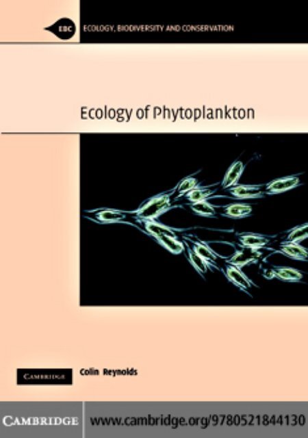
The Ecology of Phytoplankton

This page intentionally left blank

Ecology of Phytoplankton 

Phytoplankton communities dominate the pelagic 

ecosystems that cover 70% of the world’s surface 

area. In this marvellous new book Colin Reynolds 

deals with the adaptations, physiology and population 

dynamics of the phytoplankton communities 

of lakes and rivers, of seas and the great oceans. 

The book will serve both as a text and a major 

work of reference, providing basic information on 

composition, morphology and physiology of the 

main phyletic groups represented in marine and 

freshwater systems. In addition Reynolds reviews 

recent advances in community ecology, developing 

an appreciation of assembly processes, coexistence 

and competition, disturbance and diversity. Aimed 

primarily at students of the plankton, it develops 

many concepts relevant to ecology in the widest 

sense, and as such will appeal to a wide readership 

among students of ecology, limnology and oceanography. 

Born in London, Colin completed his formal education 

at Sir John Cass College, University of London. 

He worked briefly with the Metropolitan Water 

Board and as a tutor with the Field Studies Council. 

In 1970, he joined the staff at the Windermere 

Laboratory of the Freshwater Biological Association. 

He studied the phytoplankton of eutrophic meres, 

then on the renowned ‘Lund Tubes’, the large limnetic 

enclosures in Blelham Tarn, before turning his 

attention to the phytoplankton of rivers. During the 

1990s, working with Dr Tony Irish and, later, also Dr 

Alex Elliott, he helped to develop a family of models 

based on, the dynamic responses of phytoplankton 

populations that are now widely used by managers. 

He has published two books, edited a dozen others 

and has published over 220 scientific papers as 

well as about 150 reports for clients. He has 

given advanced courses in UK, Germany, Argentina, 

Australia and Uruguay. He was the winner of the 

1994 Limnetic Ecology Prize; he was awarded a coveted 

Naumann–Thienemann Medal of SIL and was 

honoured by Her Majesty the Queen as a Member of 

the British Empire. Colin also served on his municipal 

authority for 18 years and was elected mayor of 

Kendal in 1992–93.

ecology, biodiversity, and conservation 

Series editors 

Michael Usher University of Stirling, and formerly Scottish Natural Heritage 

Denis Saunders Formerly CSIRO Division of Sustainable Ecosystems, Canberra 

Robert Peet University of North Carolina, Chapel Hill 

Andrew Dobson Princeton University 

Editorial Board 

Paul Adam University of New South Wales, Australia 

H. J. B. Birks University of Bergen, Norway 

Lena Gustafsson Swedish University of Agricultural Science 

Jeff McNeely International Union for the Conservation of Nature 

R. T. Paine University of Washington 

David Richardson University of Cape Town 

Jeremy Wilson Royal Society for the Protection of Birds 

The world’s biological diversity faces unprecedented threats. The urgent challenge facing the concerned 

biologist is to understand ecological processes well enough to maintain their functioning in 

the face of the pressures resulting from human population growth. Those concerned with the conservation 

of biodiversity and with restoration also need to be acquainted with the political, social, 

historical, economic and legal frameworks within which ecological and conservation practice must 

be developed. This series will present balanced, comprehensive, up-to-date and critical reviews of 

selected topics within the sciences of ecology and conservation biology, both botanical and zoological, 

and both ‘pure’ and ‘applied’. It is aimed at advanced (final-year undergraduates, graduate 

students, researchers and university teachers, as well as ecologists and conservationists in industry, 

government and the voluntary sectors. The series encompasses a wide range of approaches and 

scales (spatial, temporal, and taxonomic), including quantitative, theoretical, population, community, 

ecosystem, landscape, historical, experimental, behavioural and evolutionary studies. The emphasis 

is on science related to the real world of plants and animals, rather than on purely theoretical 

abstractions and mathematical models. Books in this series will, wherever possible, consider issues 

from a broad perspective. Some books will challenge existing paradigms and present new ecological 

concepts, empirical or theoretical models, and testable hypotheses. Other books will explore new 

approaches and present syntheses on topics of ecological importance. 

Ecology and Control of Introduced Plants Judith H. Myers and Dawn R. Bazely 

Invertebrate Conservation and Agricultural Ecosystems T. R. New 

Risks and Decisions for Conservation and Environmental Management Mark Burgman 

Nonequilibrium Ecology Klaus Rohde 

Ecology of Populations Esa Ranta, Veijo Kaitala and Per Lundberg

The Ecology of Phytoplankton 

C. S. Reynolds

cambridge university press 

Cambridge, New York, Melbourne, Madrid, Cape Town, Singapore, São Paulo 

Cambridge University Press 

The Edinburgh Building, Cambridge cb2 2ru, UK 

Published in the United States of America by Cambridge University Press, New York 

www.cambridge.org 

Information on this title: www.cambridge.org/9780521844130 

© Cambridge University Press 2006 

This publication is in copyright. Subject to statutory exception and to the provision of 

relevant collective licensing agreements, no reproduction of any part may take place 

without the written permission of Cambridge University Press. 

First published in print format 

2006 

isbn-13 978-0-511-19094-0 eBook (EBL) 

isbn-10 0-511-19094-8 eBook (EBL) 

isbn-13 978-0-521-84413-0 hardback 

isbn-10 0-521-84413-4 hardback 

isbn-13 978-0-521-60519-9 paperback 

isbn-10 0-521-60519-9 paperback 

Cambridge University Press has no responsibility for the persistence or accuracy of urls 

for external or third-party internet websites referred to in this publication, and does not 

guarantee that any content on such websites is, or will remain, accurate or appropriate.

This book is dedicated to 

my wife, JEAN, to whom its writing 

represented an intrusion into 

domestic life, and to Charles Sinker, 

John Lund and Ramón Margalef. Each is 

a constant source of inspiration to me.

Contents 

Preface 

Acknowledgements 

page ix 

Chapter 1. Phytoplankton 1 

1.1 Definitions and terminology 1 

1.2 Historical context of phytoplankton studies 3 

1.3 The diversification of phytoplankton 4 

1.4 General features of phytoplankton 15 

1.5 The construction and composition of freshwater 

phytoplankton 24 

1.6 Marine phytoplankton 34 

1.7 Summary 36 

Chapter 2. Entrainment and distribution in the pelagic 38 

2.1 Introduction 38 

2.2 Motion in aquatic environments 39 

2.3 Turbulence 42 

2.4 Phytoplankton sinking and floating 

2.5 Adaptive and evolutionary mechanisms for 

49 

regulating ws 

53 

2.6 Sinking and entrainment in natural turbulence 67 

2.7 The spatial distribution of phytoplankton 77 


Chapter 3. Photosynthesis and carbon acquisition in 



3.2 Essential biochemistry of photosynthesis 94 

3.3 Light-dependent environmental sensitivity of 

photosynthesis 101 

3.4 Sensitivity of aquatic photosynthesis to carbon 

sources 124 

3.5 Capacity, achievement and fate of primary 

production at the ecosystem scale 131 


Chapter 4. Nutrient uptake and assimilation in 



4.2 Cell uptake and intracellular transport of 

nutrients 146 

4.3 Phosphorus: requirements, uptake, deployment in 


xii

viii CONTENTS 

4.4 Nitrogen: requirements, sources, uptake and 

metabolism in phytoplankton 161 

4.5 The role of micronutrients 166 

4.6 Major ions 171 

4.7 Silicon: requirements, uptake, deployment in 



Chapter 5. Growth and replication of phytoplankton 178 

5.1 Introduction: characterising growth 178 

5.2 The mechanics and control of growth 179 

5.3 The dynamics of phytoplankton growth and 

replication in controlled conditions 183 

5.4 Replication rates under sub-ideal conditions 189 

5.5 Growth of phytoplankton in natural 

environments 217 


Chapter 6. Mortality and loss processes in phytoplankton 239 


6.2 Wash-out and dilution 240 

6.3 Sedimentation 243 

6.4 Consumption by herbivores 250 

6.5 Susceptibility to pathogens and parasites 292 

6.6 Death and decomposition 296 

6.7 Aggregated impacts of loss processes on 

phytoplankton composition 297 


Chapter 7. Community assembly in the plankton: pattern, 

process and dynamics 302 


7.2 Patterns of species composition and temporal 

change in phytoplankton assemblages 302 

7.3 Assembly processes in the phytoplankton 350 


Chapter 8. Phytoplankton ecology and aquatic ecosystems: 

mechanisms and management 387 


8.2 Material transfers and energy flow in pelagic 

systems 387 

8.3 Anthropogenic change in pelagic environments 395 


8.5 A last word 435 

Glossary 

Units, symbols and abbreviations 

437 

440

References 

Index to lakes, rivers and seas 

Index to genera and species of 

phytoplankton 

Index to genera and species of other 

organisms 

General index 

447 

508 

511 

520 

524 

CONTENTS ix

Preface 

This is the third book I have written on the subject 

of phytoplankton ecology. When I finished 

the first, The Ecology of Freshwater Phytoplankton 

(Reynolds, 1984a), I vowed that it would also be 

my last. I felt better about it once it was published 

but, as I recognised that science was moving 

on, I became increasingly frustrated about 

the growing datedness of its information. When 

an opportunity was presented to me, in the form 

of the 1994 Ecology Institute Prize, to write my 

second book on the ecology of plankton, Vegetation 

Processes in the Pelagic (Reynolds, 1997a), I 

was able todrawontheenormous strides that 

were being made towards understanding the part 

played by the biochemistry, physiology and population 

dynamics of plankton in the overall functioning 

of the great aquatic ecosystems. Any feeling 

of satisfaction that that exercise brought to 

me has also been overtaken by events of the last 

decade, which have seen new tools deployed to 

the greater amplification of knowledge and new 

facts uncovered to be threaded into the web of 

understanding of how the world works. 

Of course, this is the way of science. There 

is no scientific text that can be closed with a 

sigh, ‘So that’s it, then’. There are always more 

questions. I actually have rather more now than 

I had at the same stage of finishing the 1984 volume. 

No, the best that can be expected, or even 

hoped for, is a periodic stocktake: ‘This is what 

we have learned, this is how we think we can 

explain things and this is where it fits into what 

we thought we knew already; this will stand until 

we learn something else.’ This is truly the way 

of science. Taking observations, verifying them 

by experimentation, moving from hypothesis to 

fact, we are able to formulate progressively closer 

approximations to the truth. 

In fact, the second violation of my 1984 vow 

has a more powerful and less high-principled 

driver. It isjustthattheprogressinplankton 

ecology since 1984 has been astounding, turning 

almost each one of the first book’s basic assumptions 

on its head. Besides widening the scope of 

the present volume to address more overtly the 

marine phytoplankton, I have set out to construct 

anew perspective on the expanded knowledge 

base. I have to say at once that the omission of 

‘freshwater’ from the new title does not imply 

that the book covers the ecology of marine plankton 

in equivalent detail. It does, however, signify 

agenuine attempt to bridge the deep but wholly 

artificial chasm that exists between marine and 

freshwater science, which political organisation 

and science funding have perpetuated. 

At apersonal level, this wider view is a satisfying 

thing to develop, being almost a plea for absolution 

– ‘I am sorry for getting it wrong before, 

this is what I should have said!’ At a wider level, I 

am conscious that many people still use and frequently 

cite my 1984 book; I would like them to 

know that I no longer believe everything, or even 

very much, of what I wrote then. As if to emphasise 

this, I have adopted a very similar approach 

to the subject, again using eight chapters (albeit 

with altered titles). These are developed according 

to a similar sequence of topics, through morphology, 

suspension, ecophysiology and dynamics 

to the structuring of communities and their 

functions within ecosystems. This arrangement 

allows me to contrast directly the new knowledge 

and the understanding it has rendered 

redundant. 

So just what are these mould-breaking 

findings? In truth, they impinge upon the subject 

matter in each of the chapters. Advances in 

microscopy have allowed ultrastructural details 

of planktic organisms to be revealed for the first 

time. The advances in molecular biology, in particular 

the introduction of techniques for isolating 

chromosomes and ribosomes, fragmenting 

them by restriction enzymes and reading genetic 

sequences, have totally altered perceptions about 

phyletic relationships among planktic taxa and 

suppositions about their evolution. The classification 

of organisms is undergoing change of revolutionary 

proportions, while morphological variation 

among (supposedly) homogeneous genotypes

xii PREFACE 

questions the very concept of putting names 

to individual organisms. At the scale of cells, 

the whole concept of how they are moved in 

the water has been addressed mathematically. 

It is now appreciated that planktic cells experience 

critical physical forces that are very different 

from those affecting (say) fish: viscosity and 

small-scale turbulence determine the immediate 

environment of microorganisms; surface tension 

is a lethal and inescapable spectre; while shear 

forces dominate dispersion and the spatial distributions 

of populations. These discoveries flow 

from the giant leaps in quantification and measurements 

made by physical limnologists and 

oceanographers since the early 1980s. These have 

also impinged on the revision of how sinking 

and settlement of phytoplankton are viewed and 

they have helped to consolidate a robust theory 

of filter-feeding by zooplankton. 

The way in which nutrients are sequestered 

from dilute and dispersed sources in the water 

and then deployed in the assembly and replication 

of new generations of phytoplankton has 

been intensively investigated by physiologists. 

Recent findings have greatly modified perceptions 

about what is meant by ‘limiting nutrients’ 

and what happens when one or other is in short 

supply. As Sommer (1996) commented, past suppositions 

about the repercussions on community 

structure have had to be revised, both through 

the direct implications for interspecific competition 

for resources and, indirectly, through the 

effects of variable nutritional value of potential 

foods to the web of dependent consumers. 

Arguably, the greatest shift in understanding 

concerns the way in which the pelagic ecosystem 

works. Although the abundance of planktic 

bacteria and the relatively vast reserve of 

dissolved organic carbon (DOC) had long been 

recognised, the microorganismic turnover of carbon 

has only been investigated intensively during 

the last two decades. It was soon recognised 

that the metazoan food web of the open 

oceans is linked to the producer network via 

the turnover of the microbes and that this statement 

applies to many larger freshwater systems 

as well. The metabolism of the variety of substances 

embraced by ‘DOC’ varies with source and 

chain length but a labile fraction originates from 

phytoplankton photosynthesis that is leaked or 

actively discharged into the water. Far from holding 

to the traditional view of the pelagic food 

chain – algae, zooplankton, fish – plankton ecologists 

now have to acknowledge that marine 

food webs are regulated ‘by a sea of microbes’ 

(Karl, 1999), through the muliple interactions of 

organic and inorganic resources and by the lock 

of protistan predators and acellular pathogens 

(Smetacek, 2002). Even in lakes, where the case 

for the top–down control of phytoplankton by 

herbivorous grazers is championed, the otherwise 

dominant microbially mediated supply of 

resources to higher trophic levels is demonstrably 

subsidised by components from the littoral 

(Schindler et al., 1996; Vadeboncoeur et al., 2002). 

There have been many other revolutions. One 

more to mention here is the progress in ecosystem 

ecology, or more particularly, the bridge 

between the organismic and population ecology 

and the behaviour of entire systems. How ecosystems 

behave, how their structure is maintained 

and what is critical to that maintenance, what 

the biogeochemical consequences might be and 

how they respond to human exploitation and 

management, have all become quantifiable. The 

linking threads are based upon thermodynamic 

rules of energy capture, exergy storage and structural 

emergence, applied through to the systems 

level (Link, 2002; Odum, 2002). 

In the later chapters in this volume, I attempt 

to apply these concepts to phytoplankton-based 

systems, where the opportunity is again taken 

to emphasise the value to the science of ecology 

of studying the dynamics of microorganisms 

in the pursuit of high-order pattern and assembly 

rules (Reynolds, 1997, 2002b). The dual challenge 

remains, to convince students of forests 

and other terrestrial ecosystems that microbial 

systems do conform to analogous rules, albeit 

at very truncated real-time scales, and to persuade 

microbiologists to look up from the microscope 

for long enough to see how their knowledge 

might be applied to ecological issues. 

Iamproud to acknowledge the many people 

who have influenced or contributed to the subject 

matter of this book. I thank Charles Sinker 

for inspiring a deep appreciation of ecology and 

its mechanisms. I am grateful to John Lund, CBE,

FRS for the opportunity to work on phytoplankton 

asapostgraduate and for the constant inspiration 

and access to his knowledge that he has 

given me. Of the many practising theoretical ecologists 

whose works I have read, I have felt the 

greatest affinity to the ideas and logic of Ramón 

Margalef; I greatly enjoyed the opportunities to 

discuss these with him and regret that there will 

be no more of them. 

I gratefully acknowledge the various scientists 

whose work has profoundly influenced particular 

parts of this book and my thinking generally. 

They include (in alphabetical order) Sallie 

Chisholm, Paul Falkowski, Maciej Gliwicz, 

Phil Grime, Alan Hildrew, G. E. Hutchinson, Jörg 

Imberger, Petur Jónasson, Sven-Erik Jørgensen, 

Dave Karl, Winfried Lampert, John Lawton, John 

Raven, Marten Scheffer, Ted Smayda, Milan 

Straˇskraba, Reinhold Tüxen, Anthony Walsby and 

Thomas Weisse. I have also been most fortunate 

in having been able, at various times, to 

work with and discuss many ideas with colleagues 

who include Keith Beven, Sylvia Bonilla, 

Odécio Cáceres, Paul Carling, Jean-Pierre Descy, 

Mónica Diaz, Graham Harris, Vera Huszar, Dieter 

Imboden, Kana Ishikawa, Medina Kadiri, Susan 

Kilham, Michio Kumagai, Bill Li, Vivian Montecino, 

Mohi Munawar, Masami Nakanishi, Shin- 

Ichi Nakano, Luigi Naselli-Flores, Pat Neale, Søren 

Nielsen, Judit Padisák, Fernando Pedrozo, Victor 

Smetaček, Ulrich Sommer, José Tundisi and 

Peter Tyler. I am especially grateful to Catherine 

Legrand who generously allowed me to use 

and interpret her experimental data on Alexandrium. 

Nearer to home, I have similarly benefited 

from long and helpful discussions with such erstwhile 

Windermere colleagues as Hilda Canter- 

Lund, Bill Davison, Malcolm Elliott, Bland Finlay, 

Glen George, Ivan Heaney, Stephen Maberly, Jack 

Talling and Ed Tipping. 

During my years at The Ferry House, I was 

ably and closely supported by several co-workers, 

PREFACE xiii 

among whom special thanks are due to Tony 

Irish, Sheila Wiseman, George Jaworski and Brian 

Godfrey. Peter Allen, Christine Butterwick, Julie 

Corry (later Parker), Mitzi De Ville, Joy Elsworth, 

Alastair Ferguson, Mark Glaister, David Gouldney, 

Matthew Rogers, Stephen Thackeray and Julie 

Thompson also worked with me at particular 

times. Throughout this period, I was privileged 

to work in a ‘well-found’ laboratory with abundant 

technical and practical support. I freely 

acknowledge use of the world’s finest collection 

of the freshwater literature and the assistance 

provided at various times by John Horne, Ian 

Pettman, Ian McCullough, Olive Jolly and Marilyn 

Moore. Secretarial assistance has come from 

Margaret Thompson, Elisabeth Evans and Joyce 

Hawksworth. Trevor Furnass has provided abundant 

reprographic assistance over many years. I 

am forever in the debt of Hilda Canter-Lund, FRPS 

for the use of her internationally renowned photomicrographs. 

Aspecial word is due to the doctoral students 

whom I have supervised. The thirst for knowledge 

and understanding of a good pupil generally 

provide a foil and focus in the other direction. 

I owe much to the diligent curiosity of Chris 

van Vlymen, Helena Cmiech, Karen Saxby (now 

Rouen), Siân Davies, Alex Elliott, Carla Kruk and 

Phil Davis. 

My final word of appreciation is reserved for 

acknowledgement of the tolerance and forbearance 

of my wife and family. I cheered through 

many juvenile football matches and dutifully 

attended a host of ballet and choir performances 

and, yes, it was quite fun to relive three more 

school curricula. Nevertheless, my children had 

less of my time than they were entitled to expect. 

Jean has generously shared with my science the 

full focus of my attention. Yet, in 35 years of marriage, 

she has never once complained, nor done 

less than encourage the pursuit of my work. I am 

proud to dedicate this book to her.

Acknowledgements 

Except where stated, the illustrations in this book 

are reproduced, redrawn or otherwise slightly 

modified from sources noted in the individual 

captions. The author and the publisher are grateful 

to the various copyright holders, listed below, 

who have given permission to use copyright material 

in this volume. While every effort has been 

made to clear permissions as appropriate, the 

publisher would appreciate notification of any 

omission. 

Figures 1.1 to 1.8, 1.10, 2.8 to 2.13, 2.17, 2.20 to 

2.31, 3.3 to 3.9, 3.16 and 3.17, 5.20, 6.2, 6.7, 6.11. 

7.6 and 7.18 are already copyrighted to Cambridge 

University Press. 

Figure 1.9 is redrawn by permission of Oxford 


Figure 1.11 is the copyright of the American Society 

of Limnology and Oceanography. 

Figures 2.1 and 2.2, 2.5 to 2.7, 2.15 and 2.16, 2.18 

and 2.19, 3.12, 3.14, 3.19, 4.1, 4.3 to 4.5, 5.1 to 

5.5, 5.8, 5.10, 5.12 and 5.13, 5.20 and 5.21, 6.1, 

6.2, 6.4, 6.14, 7.8, 7.10 and 7.11, 7.14, 7.16 and 7.17, 

7.20 and 7.22 are redrawn by permission of The 

Ecology Institute, Oldendorf. 

Figures 2.3 and 4.7 are redrawn from the source 

noted in the captions, with acknowledgement to 

Artemis Press. 

Figures 2.4, 3.18, 5.11, 5.18, 7.5, 7.15, 8.2 and 8.3 

are redrawn from the various sources noted in 

the respective captions and with acknowledgement 

to Elsevier Science, B.V. 

Figure 2.14 is redrawn from the British Phycological 

Journal by permission of Taylor & Francis Ltd 

(http://www.tandf.co.uk/journals). 

Figure 3.1 is redrawn by permission of Nature 

Publishing Group. 

Figures 3.2, 3.11, 3.13, 4.2, 5.6, 6.4, 6.6, 6.9, 

6.10 and 6.13 come from various titles that are 

the copyright of Blackwell Science (the specific 

sources are noted in the figure captions) and are 

redrawn by permission. 

Figures 3.7, 3.15, 4.6 and 7.2.3 (or parts thereof) 

are redrawn from Freshwater Biology by permission 

of Blackwell Science. 

Figure 3.7 incorporates items redrawn from Biological 

Reviews with acknowledgement to the Cambridge 

Philosophical Society. 

Figure 5.9 is redrawn by permission of John Wiley 

& Sons Ltd. 

Figure 5.14 is redrawn by permission of Springer- 

Verlag GmbH. 

Figures 5.15 to 5.17, 5.19, 6.8 and 6.9 are redrawn 

by permission of SpringerScience+Business BV. 

Figures 6.12, 6.15, 7.1 to 7.4, 7.9 and 8.6 are reproduced 

from Journal of Plankton Research by permission 

of Oxford University Press. Dr K. Bruning also 

gave permission to produce Fig. 6.12. 

Figure 7.7 is redrawn by permission of the Director, 

Marine Biological Association. 

Figures 7.12 to 7.14, 7.24 and 7.25 are redrawn 

from Verhandlungen der internationale Vereinigung 

für theoretische und angewandte Limnologie 

by permission of Dr E. Nägele (Publisher) 

(http://www.schwezerbart.de). 

Figure 7.19 is redrawn with acknowledgement to 

the Athlone Press of the University of London. 

Figure 7.21 is redrawn from Aquatic Ecosystems 

Health and Management by permission of Taylor 

&Francis, Inc. (http://www.taylorandfrancis.com). 

Figure 8.1 is redrawn from Scientia Maritima by 

permission of Institut de Ciències del Mar. 

Figures 8.5, 8.7 and 8.8 are redrawn by permission 

of the Chief Executive, Freshwater Biological 

Association.

Chapter 1 

Phytoplankton 

1.1 Definitions and terminology 

The correct place to begin any exposition of a 

major component in biospheric functioning is 

with precise definitions and crisp discrimination. 

This should be a relatively simple exercise but for 

the need to satisfy a consensus of understanding 

and usage. Particularly among the biological 

sciences, scientific knowledge is evolving rapidly 

and, as it does so, it often modifies and outgrows 

the constraints of the previously acceptable terminology. 

I recognised this problem for plankton 

science in an earlier monograph (Reynolds, 

1984a). Since then, the difficulty has worsened 

and it impinges on many sections of the present 

book. The best means of dealing with it is to 

accept the issue as a symptom of the good health 

and dynamism of the science and to avoid constraining 

future philosophical development by a 

redundant terminological framework. 

The need for definitions is not subverted, however, 

but it transforms to an insistence that those 

that are ventured are provisional and, thus, open 

to challenge and change. To be able to reveal 

something also of the historical context of the 

usage is to give some indication of the limitations 

of the terminology and of the areas of conjecture 

impinging upon it. 

So it is with ‘plankton’. The general understanding 

of this term is that it refers to the collective 

of organisms that are adapted to spend part 

or all of their lives in apparent suspension in the 

open water of the sea, of lakes, ponds and rivers. 

The italicised words are crucial to the concept 

and are not necessarily contested. Thus, ‘plankton’ 

excludes other suspensoids that are either 

non-living, such as clay particles and precipitated 

chemicals, or are fragments or cadavers derived 

from biogenic sources. Despite the existence of 

thenow largely redundant subdivision tychoplankton 

(see Box 1.1), ‘plankton’ normally comprises 

those living organisms that are only fortuitously 

and temporarily present, imported from adjacent 

habitats but which neither grew in this habitat 

nor are suitably adapted to survive in the truly 

open water, ostensibly independent of shore and 

bottom. Such locations support distinct suites of 

surface-adhering organisms with their own distinctive 

survival adaptations. 

‘Suspension’ has been more problematic, having 

quite rigid physical qualifications of density 

and movement relative to water. As will be 

rehearsed in Chapter 2, only rarely can plankton 

be isopycnic (having the same density) with 

the medium and will have a tendency to float 

upwards or sink downwards relative to it. The 

rate of movement is also size dependent, so 

that ‘apparent suspension’ is most consistently 

achieved by organisms of small (

2 PHYTOPLANKTON 

In this way, plankton comprises organisms 

that range in size from that of viruses (a few tens 

of nanometres) to those of large jellyfish (a metre 

or more). Representative organisms include bacteria, 

protistans, fungi and metazoans. In the 

past, it has seemed relatively straightforward to 

separate the organisms of the plankton, both 

into broad phyletic categories (e.g. bacterioplankton, 

mycoplankton) or into similarly broad functional 

categories (photosynthetic algae of the 

phytoplankton, phagotrophic animals of the zooplankton). 

Again, as knowledge of the organ- 

Box 1.1 Some definitions used in the literaure 

on plankton 

seston the totality of particulate matter in water; all material not 

in solution 

tripton non-living seston 

plankton living seston, adapted for a life spent wholly or partly in 

quasi-suspension in open water, and whose powers of 

motility do not exceed turbulent entrainment (see 

Chapter 2) 

nekton animals adapted to living all or part of their lives in open 

water but whose intrinsic movements are almost 

independent of turbulence 

euplankton redundant term to distinguish fully adapted, truly planktic 

organisms from other living organisms fortuitously 

present in the water 

tychoplankton non-adapted organisms from adjacent habitats and 

present in the water mainly by chance 

meroplankton planktic organisms passing a major part of the life history 

out of the plankton (e.g. on the bottom sediments) 

limnoplankton plankton of lakes 

heleoplankton plankton of ponds 

potamoplankton plankton of rivers 

phytoplankton planktic photoautotrophs and major producer of the 

pelagic 

bacterioplankton planktic prokaryotes 

mycoplankton planktic fungi 

zooplankton planktic metazoa and heterotrophic protistans 

Some more, now redundant, terms 

The terms nannoplankton, ultraplankton, µ-algae are older names for various smaller 

size categories of phytoplankton, eclipsed by the classification of Sieburth et al. 

(1978) (see Box 1.2). 

isms, their phyletic affinities and physiological 

capabilities has expanded, it has become clear 

that the divisions used hitherto do not precisely 

coincide: there are photosynthetic bacteria, 

phagotrophic algae and flagellates that take 

up organic carbon from solution. Here, as in general, 

precision will be considered relevant and 

important in the context of organismic properties 

(their names, phylogenies, their morphological 

and physiological characteristics). On the 

other hand, the generic contributions to systems 

(at the habitat or ecosystem scales) of the

photosynthetic primary producers, phagotrophic 

consumers and heterotrophic decomposers may 

be attributed reasonably but imprecisely to phytoplankton, 

zooplankton and bacterioplankton. 

The defintion of phytoplankton adopted for 

this book is the collective of photosynthetic 

microorganisms, adapted to live partly or continuously 

in open water. As such, it is the photoautotrophic 

part of the plankton and a major primary 

producer of organic carbon in the pelagic 

of the seas and of inland waters. The distinction 

of phytoplankton from other categories of plankton 

and suspended matter are listed in Box 1.1. 

It may be added that it is correct to refer to 

phytoplankton as a singular term (‘phytoplankton 

is’ rather than ‘phytoplankton are’). A single 

organism is a phytoplanktont or (more ususally) 

phytoplankter. Incidentally, the adjective ‘planktic’ 

is etymologically preferable to the more commonly 

used ‘planktonic’. 

1.2 Historical context of 

phytoplankton studies 

The first use of the term ‘plankton’ is attributed 

in several texts (Ruttner, 1953; Hutchinson, 1967) 

to Viktor Hensen, who, in the latter half of the 

nineteenth century, began to apply quantitative 

methods to gauge the distribution, abundance 

and productivity of the microscopic organisms 

of the open sea. The monograph that is usually 

cited (Hensen, 1887) is, in fact, rather obscure 

and probably not well read in recent times but 

Smetacek et al. (2002) haveprovidedaprobing 

and engaging review of the original, within the 

context of early development of plankton science. 

Most of the present section is based on their 

article. 

The existence of a planktic community of 

organisms in open water had been demonstrated 

many years previously by Johannes Müller. Knowledge 

of some of the organisms themselves 

stretches further back, to the earliest days 

of microscopy. From the 1840s, Müller would 

demonstrate net collections to his students, using 

the word Auftrieb to characterise the community 

(Smetacek et al., 2002). The literal transla- 

HISTORICAL CONTEXT OF PHYTOPLANKTON STUDIES 3 

tion to English is ‘up drive’, approximately ‘buoyancy’ 

or ‘flotation’, a clear reference to Müller’s 

assumption that the material floated up to the 

surface waters – like so much oceanic dirt! It 

took one of Müller’s students, Ernst Haeckel, to 

champion the beauty of planktic protistans and 

metazoans. His monograph on the Radiolaria 

was also one of the first to embrace Darwin’s 

(1859) evolutionary theory in order to show 

structural affinities and divergences. Haeckel, of 

course, became best known for his work on 

morphology, ontogeny and phylogeny. According 

to Smetacek et al. (2002), his interest and skills 

as a draughtsman advanced scientific awareness 

of the range of planktic form (most significantly, 

Haeckel, 1904) but to the detriment of any real 

progress in understanding of functional differentiation. 

Until the late 1880s, it was not appreciated 

that the organisms of the Auftrieb, eventhe 

algae among them, could contribute much to the 

nutrition of the larger animals of the sea. Instead, 

it seems to have been supposed that organic matter 

inthe fluvial discharge from the land was the 

major nutritive input. It is thus rather interesting 

to note that, a century or so later, this possibility 

has enjoyed something of a revival (see 

Chapters 3 and 8). 

If Haeckel had conveyed the beauty of the 

pelagic protistans, it was certainly Viktor Hensen 

who had been more concerned about their role 

in a functional ecosystem. Hensen was a physiologist 

who brought a degree of empiricism 

to his study of the perplexing fluctuations in 

North Sea fish stocks. He had reasoned that 

fish stocks and yields were related to the production 

and distribution of the juvenile stages. 

Through devising techniques for sampling, quantification 

and assessing distribution patterns, 

always carefully verified by microscopic examination, 

Hensen recognised both the ubiquity of 

phytoplankton and its superior abundance and 

quality over coastal inputs of terrestrial detritus. 

He saw the connection between phytoplankton 

and the light in the near-surface layer, the nutritive 

resource it provided to copepods and other 

small animals, and the value of these as a food 

source to fish. 

Thus, in addition to bequeathing a new 

name for the basal biotic component in pelagic


ecosystems, Hensen may be regarded justifiably 

as the first quantitative plankton ecologist and 

as the person who established a formal methodology 

for its study. Deducing the relative contributions 

of Hensen and Haeckel to the foundation 

of modern plankton science, Smetacek et al. 

(2002) concluded that it is the work of the latter 

that has been the more influential. This is an 

opinion with which not everyone will agree but 

this is of little consequence. However, Smetacek 

et al.(2002)offeredamostprofoundandresonant 

observation in suggesting that Hensen’s general 

understanding of the role of plankton (‘the big 

picture’) was essentially correct but erroneous in 

its details, whereas in Haeckel’s case, it was the 

other way round. Nevertheless, both have good 

claim to fatherhood of plankton science! 

1.3 The diversification of 

phytoplankton 

Current estimates suggest that between 4000 and 

5000 legitimate species of marine phytoplankton 

have been described (Sournia et al. 1991; 

Tett and Barton, 1995). I have not seen a comparable 

estimate for the number of species in 

inland waters, beyond the extrapolation I made 

(Reynolds, 1996a) thatthenumberisunlikelyto 

be substantially smaller. In both lists, there is 

not just a large number of mutually distinct taxa 

of photosynthetic microorganisms but there is a 

wide variety of shape, size and phylogenetic affinity. 

As has also been pointed out before (Reynolds, 

1994a), the morphological range is comparable to 

the one spanning forest trees and the herbs that 

grow at their base. The phyletic divergence of the 

representatives is yet wider. It would be surprising 

if the species of the phytoplankton were uniform 

in their requirements, dynamics and susceptibilities 

to loss processes. Once again, there 

is a strong case for attempting to categorise the 

phytoplankton both on the phylogeny of organisms 

and on the functional basis of their roles in 

aquatic ecosystems. Both objectives are adopted 

for the writing of this volume. Whereas the former 

is addressed only in the present chapter, the 

latter quest occupies most of the rest of the book. 

However, it is not giving away too much to anticipate 

that systematics provides an important foundation 

for species-specific physiology and which 

is itself part-related to morphology. Accordingly, 

great attention is paid here to the differentiation 

of individualistic properties of representative 

species of phytoplankton. 

However, there is value in being able simultaneously 

to distinguish among functional categories 

(trees from herbs!). The scaling system and 

nomenclature proposed by Sieburth et al. (1978) 

has been widely adopted in phytoplankton ecology 

to distinguish functional separations within 

the phytoplankton. It has also eclipsed the use of 

such terms as µ-algae and ultraplankton to separate 

the lower size range of planktic organisms from 

those (netplankton) large enough to be retained 

by the meshes of a standard phytoplankton net. 

The scheme of prefixes has been applied to size 

categories of zooplankton, with equal success. 

The size-based categories are set out in Box 1.2. 

At the level of phyla, the classification of 

the phytoplankton is based on long-standing criteria, 

distinguished by microscopists and biochemists 

over the last 150 years or so, from 

which there is little dissent. In contrast, subdivision 

within classes, orders etc., and the tracing 

of intraphyletic relationships, affinities within 

and among families, even the validity of supposedly 

well-characterised species, has become subject 

to massive reappraisal. The new factor that 

has come into play is the powerful armoury of 

the molecular biologists, including the methods 

for reading gene sequences and for the statistical 

matching of these to measure the closeness 

to other species. 

Of course, the potential outcome is a much 

more robust, genetically verified family tree of 

authentic species of phytoplankton. This may be 

some years away. For the present, it seems pointless 

to reproduce a detailed classification of the 

phytoplankton that will soon be made redundant. 

Even the evolutionary connectivities among 

the phyla and their relationship to the geochemical 

development of the planetary structures 

are undergoing deep re-evaluation (Delwiche, 

2000; Falkowski, 2002). For these reasons, the

THE DIVERSIFICATION OF PHYTOPLANKTON 5 

Box 1.2 The classification of phytoplankton according to 

the scaling nomenclature of Sieburth et al. (1978) 

Maximum linear dimension Name a 

0.2–2 µm picophytoplankton 

2–20 µm nanophytoplankton 

20–200 µm microphytoplankton 

200 µm–2 mm mesophytoplankton 

>2 mm macrophytoplankton 

a The prefixes denote the same size categories when used with ‘-zooplankton’, ‘-algae’, ‘-cyanobacteria’, 

‘flagellates’, etc. 

taxonomic listings in Table 1.1 are deliberately 

conservative. 

Although the life forms of the plankton 

include acellular microorganisms (viruses) and a 

range of well-characterised Archaea (the halobacteria, 

methanogens and sulphur-reducing bacteria, 

formerly comprising the Archaebacteria), 

the most basicphotosynthetic organisms of the 

phytoplankton belong to the Bacteria (formerly, 

Eubacteria). The separation of the ancestral bacteria 

from thearchaeans (distinguished by the 

possession of membranes formed of branched 

hydrocarbons and ether linkages, as opposed to 

the straight-chain fatty acids and ester linkages 

found in the membranes of all other organisms: 

Atlas and Bartha, 1993) occurred early in microbial 

evolution (Woese, 1987; Woeseet al., 1990). 

The appearance of phototrophic forms, distinguished 

by their crucial ability to use light 

energy in order to synthesise adenosine triphosphate 

(ATP) (see Chapter 3), was also an ancient 

event that took place some 3000 million years ago 

(3 Ga BP (before present)). Some of these organisms 

were photoheterotrophs, requiring organic 

precursors for the synthesis of their own cells. 

Modern forms include green flexibacteria (Chloroflexaceae) 

and purple non-sulphur bacteria 

(Rhodospirillaceae), which contain pigments similar 

to chlorophyll (bacteriochlorophyll a, b or 

c). Others were true photoautotrophs, capable 

of reducing carbon dioxide as a source of cell 

carbon (photosynthesis). Light energy is used to 

strip electrons from a donor substance. In most 

modern plants, water is the source of reductant 

electrons and oxygen is liberated as a by-product 

(oxygenic photosynthesis). Despite their phyletic 

proximity to the photoheterotrophs and sharing 

a similar complement of bacteriochlorophylls 

(Béjà et al., 2002), the Anoxyphotobacteria 

use alternative sources of electrons and, 

in consequence, generate oxidation products 

other than oxygen (anoxygenic photosynthesis). 

Their modern-day representatives are the purple 

and green sulphur bacteria of anoxic sediments. 

Some of these are planktic in the sense that 

they inhabit anoxic, intensively stratified layers 

deep in small and suitably stable lakes. The trait 

might be seen as a legacy of having evolved in a 

wholly anoxic world. However, aerobic, anoxygenic 

phototrophic bacteria, containing bacterichlorophyll 

a, havebeenisolatedfromoxic 

marine environments (Shiba et al., 1979); it has 

also become clear that their contribution to the 

oceanic carbon cycle is not necessarily insignificant 

(Kolber et al., 2001; Goericke, 2002). 

Nevertheless, the oxygenic photosynthesis pioneered 

by the Cyanobacteria from about 2.8 Ga 

before present has proved to be a crucial step in 

the evolution of life in water and, subsequently, 

on land. Moreover, the composition of the atmosphere 

was eventually changed through the biological 

oxidation of water and the simultaneous 

removal and burial of carbon in marine sediments 

(Falkowski, 2002). Cyanobacterial photosynthesis 

is mediated primarily by chlorophyll 

a, borne on thylakoid membranes. Accessory


Table 1.1 Survey of the organisms in the phytoplankton 

Domain: BACTERIA 

Division: Cyanobacteria (blue-green algae) 

Unicellular and colonial bacteria, lacking membrane bound plastids. Primary 

photosynthetic pigment is chlorophyll a, with accessory phycobilins (phycocyanin, 

phycoerythrin). Assimilation products, glycogen, cyanophycin. Four main sub-groups, 

of which three have planktic representatives. 

Order: CHROOCOCCALES 

Unicellular or coenobial Cyanobacteria but never filamentous. Most planktic genera 

form mucilaginous colonies, and these are mainly in fresh water. Picophytoplanktic 

forms abundant in the oceans. 

Includes: Aphanocapsa, Aphanothece, Chroococcus, Cyanodictyon, 

Gomphosphaeria, Merismopedia, Microcystis, Snowella, Synechococcus, 

Synechocystis, Woronichinia 

Order: OSCILLATORIALES 

Uniseriate–filamentous Cyanobacteria whose cells all undergo division in the same 

plane. Marine and freshwater genera. 

Includes: Arthrospira, Limnothrix, Lyngbya, Planktothrix, Pseudanabaena, Spirulina, 

Trichodesmium, Tychonema 

Order: NOSTOCALES 

Unbranched–filamentous Cyanobacteria whose cells all undergo division in the same 

plane and certain of which may be facultatively differentiated into heterocysts. In the 

plankton of fresh waters and dilute seas. 

Includes: Anabaena, Anabaenopsis, Aphanizomenon, Cylindrospermopsis, 

Gloeotrichia, Nodularia 

Exempt Division: Prochlorobacteria 

Order: PROCHLORALES 

Unicellular and colonial bacteria, lacking membrane-bound plastids. Photosynthetic 

pigments are chlorophyll a and b, but lack phycobilins. 

Includes: Prochloroccus, Prochloron, Prochlorothrix 

Division: Anoxyphotobacteria 

Mostly unicellular bacteria whose (anaerobic) photosynythesis depends upon an 

electron donor other than water and so do not generate oxygen. Inhabit anaerobic 

sediments and (where appropriate) water layers where light penetrates sufficiently. 

Two main groups: 

Family: Chromatiaceae (purple sulphur bacteria) Cells able to photosynthesise 

with sulphide as sole electron donor. Cells contain bacteriochlorophyll a, b or c. 

Includes: Chromatium, Thiocystis, Thiopedia. 

Family: Chlorobiaceae (green sulphur bacteria) Cells able to photosynthesise 

with sulphide as sole electron donor. Cells contain bacteriochlorophyll a, b or c. 

Includes: Chlorobium, Clathrocystis, Pelodictyon. 

Domain: EUCARYA 

Phylum: Glaucophyta 

Cyanelle-bearing organisms, with freshwater planktic representatives. 

Includes: Cyanophora, Glaucocystis. 

Phylum: Prasinophyta 

Unicellular, mostly motile green algae with 1–16 laterally or apically placed flagella, 

cell walls covered with fine scales and plastids containing chlorophyll a and b. 

Assimilatory products mannitol, starch. 

(cont.)

Table 1.1 (cont.) 


CLASS: Pedinophyceae 

Order: PEDINOMONADALES 

Small cells, with single lateral flagellum. 

Includes: Pedinomonas 

CLASS: Prasinophyceae 

Order: CHLORODENDRALES 

Flattened, 4-flagellated cells. 

Includes: Nephroselmis, Scherffelia (freshwater); Mantoniella, Micromonas 

(marine) 

Order: PYRAMIMONADALES 

Cells with 4 or 8 (rarely 16) flagella arising from an anterior depression. Marine 

and freshwater. 

Includes: Pyramimonas 

Order: SCOURFIELDIALES 

Cells with two, sometimes unequal, flagella. Known from freshwater ponds. 

Includes: Scourfieldia 

Phylum: Chlorophyta (green algae) 

Green-pigmented, unicellular, colonial, filamentous, siphonaceous and thalloid 

algae. One or more chloroplasts containing chlorophyll a and b. Assimilation 

product, starch (rarely, lipid). 

CLASS: Chlorophyceae 

Several orders of which the following have planktic representatives: 

Order: TETRASPORALES 

Non-flagellate cells embedded in mucilaginous or palmelloid colonies, but with 

motile propagules. 

Includes: Paulschulzia, Pseudosphaerocystis 

Order: VOLVOCALES 

Unicellular or colonial biflagellates, cells with cup-shaped chloroplasts. 

Includes: Chlamydomonas, Eudorina, Pandorina, Phacotus, Volvox (in fresh 

waters); Dunaliella, Nannochloris (marine) 

Order: CHLOROCOCCALES 

Non-flagellate, unicellular or coenobial (sometimes mucilaginous) algae, with 

many planktic genera. 

Includes: Ankistrodesmus, Ankyra, Botryococcus, Chlorella, 

Coelastrum, Coenochloris, Crucigena, Choricystis, Dictyosphaerium, 

Elakatothrix, Kirchneriella, Monorophidium, Oocystis, Pediastrum, 

Scenedesmus, Tetrastrum 

Order: ULOTRICHALES 

Unicellular or mostly unbranched filamentous with band-shaped chloroplasts. 

Includes: Geminella, Koliella, Stichococcus 

Order: ZYGNEMATALES 

Unicellular or filamentous green algae, reproducing isogamously by conjugation. 

Planktic genera are mostly members of the Desmidaceae, mostly unicellular or 

(rarely) filmentous coenobia with cells more or less constricted into two 

semi-cells linked by an interconnecting isthmus. Exclusively freshwater genera. 

Includes: Arthrodesmus, Closterium, Cosmarium, Euastrum, Spondylosium, 

Staurastrum, Staurodesmus, Xanthidium 

(cont.)



Phylum: Euglenophyta 

Green-pigmented unicellular biflagellates. Plastids numerous and irregular, 

containing chlorophyll a and b. Reproduction by longitudinal fission. Assimilation 

product, paramylon, oil. One Class, Euglenophyceae, with two orders. 

Order: EUTREPTIALES 

Cells having two emergent flagella, of approximately equal length. Marine and 

freshwater species. 

Includes: Eutreptia 

Order: EUGLENALES 

Cells having two flagella, one very short, one long and emergent. 

Includes: Euglena, Lepocinclis, Phacus, Trachelmonas 

Phylum: Cryptophyta 

Order: CRYPTOMONADALES 

Naked, unequally biflagellates with one or two large plastids, containing 

chlorophyll a and c2 (but not chlorophyll b); accessory phycobiliproteins or other 

pigments colour cells brown, blue, blue-green or red; assimilatory product, 

starch. Freshwater and marine species. 

Includes: Chilomonas, Chroomonas, Cryptomonas, Plagioselmis, Pyrenomonas, 

Rhodomonas 

Phylum: Raphidophyta 

Order: RAPHIDOMONADALES (syn. CHLOROMONADALES) 

Biflagellate, cellulose-walled cells; two or more plastids containing chlorophyll a; 

cells yellow-green due to predominant accessory pigment, diatoxanthin; 

assimilatory product, lipid. Freshwater. 

Includes: Gonyostomum 

Phylum: Xanthophyta (yellow-green algae) 

Unicellular, colonial, filamentous and coenocytic algae. Motile species generally 

subapically and unequally biflagellated; two or many more discoid plastids per cell 

containing chlorophyll a. Cells mostly yellow-green due to predominant 

accessory pigment, diatoxanthin; assimilation product, lipid. Several orders, two 

with freshwater planktic representatives. 

Order: MISCHOCOCCALES 

Rigid-walled, unicellular, sometimes colonial xanthophytes. 

Includes: Goniochloris, Nephrodiella, Ophiocytium 

Order: TRIBONEMATALES 

Simple or branched uniseriate filamentous xanthophytes. 

Includes: Tribonema 

Phylum: Eustigmatophyta 

Coccoid unicellular, flagellated or unequally biflagellated yellow-green algae with 

masking of chlorophyll a by accessory pigment violaxanthin. Assimilation product, 

probably lipid. 

Includes: Chlorobotrys, Monodus 

Phylum: Chrysophyta (golden algae) 

Unicellular, colonial and filamentous. often uniflagellate, or unequally biflagellate 

algae. Contain chlorophyll a, c1 and c2, generally masked by abundant accessory 

pigment, fucoxanthin, imparting distinctive golden colour to cells. Cells 

sometimes naked or or enclosed in an urn-shaped lorica, sometimes with 

siliceous scales. Assimilation products, lipid, leucosin. Much reclassified group, has 

several classes and orders in the plankton. 

(cont.)



CLASS: Chrysophyceae 

Order: CHROMULINALES 

Mostly planktic, unicellular or colony-forming flagellates with one or two 

unequal flagella, occasionally naked, often in a hyaline lorica or gelatinous 

envelope. 

Includes: Chromulina, Chrysococcus, Chrysolykos, Chrysosphaerella, Dinobryon, 

Kephyrion, Ochromonas, Uroglena 

Order: HIBBERDIALES 

Unicellular or colony-forming epiphytic gold algae but some planktic 

representatives. 

Includes: Bitrichia 

CLASS: Dictyochophyceae 

Order: PEDINELLALES 

Radially symmetrical, very unequally biflagellate unicells or coenobia. 

Includes: Pedinella (freshwater); Apedinella, Pelagococcus, Pelagomonas, 

Pseudopedinella (marine) 

CLASS: Synurophyceae 

Order: SYNURALES 

Unicellular or colony-forming flagellates, bearing distinctive siliceous scales. 

Includes: Mallomonas, Synura 

Phylum: Bacillariophyta (diatoms) 

Unicellular and coenobial yellow-brown, non-motile algae with numerous discoid 

plastids, containing chlorophyll a, c1 and c2, masked by accessory pigment, 

fucoxanthin. Cell walls pectinaceous, in two distinct and overlapping halves, and 

impregnated with cryptocrystalline silica. Assimilatory products, chrysose, lipids. 

Two large orders, both conspicuously represented in the marine and freshwater 

phytoplankton. 

CLASS: Bacillariophyceae 

Order: BIDDULPHIALES (centric diatoms) 

Diatoms with cylindrical halves, sometimes well separated by girdle bands. Some 

species form (pseudo-)filaments by adhesion of cells at their valve ends. 

Includes: Aulacoseira, Cyclotella, Stephanodiscus, Urosolenia (freshwater); 

Cerataulina, Chaetoceros, Detonula, Rhizosolenia, Skeletonema, Thalassiosira 

(marine) 

Order: BACILLARIALES (pennate diatoms) 

Diatoms with boat-like halves, no girdle bands. Some species form coenobia by 

adhesion of cells on their girdle edges. 

Includes: Asterionella, Diatoma, Fragilaria, Synedra, Tabellaria (freshwater); 

Achnanthes, Fragilariopsis, Nitzschia (marine) 

Phylum: Haptophyta 

CLASS: Haptophyceae 

Gold or yellow-brown algae, usually unicellular, with two subequal flagella and a 

coiled haptonema, but with amoeboid, coccoid or palmelloid stages. Pigments, 

chlorophyll a, c1 and c2, masked by accessory pigment (usually fucoxanthin). 

Assimilatory product, chrysolaminarin. Cell walls with scales, sometimes more or 

less calcified. 

Order: PAVLOVALES 

Cells with haired flagella and small haptonema. Marine and freshwater species. 

Includes: Diacronema, Pavlova 

(cont.)



Order: PRYMNESIALES 

Cells with smooth flagella, haptonema usually small. Mainly marine or brackish 

but some common in freshwater plankton. 

Includes: Chrysochromulina, Isochrysis, Phaeocystis, Prymnesium 

Order: COCCOLITHOPHORIDALES 

Cell suface covered by small, often complex, flat calcified scales (coccoliths). 

Exclusively marine. 

Include: Coccolithus, Emiliana, Florisphaera, Gephyrocapsa, Umbellosphaera 

Phylum: Dinophyta 

Mostly unicellular, sometimes colonial, algae with two flagella of unequal length 

and orientation. Complex plastids containing chlorophyll a, c1 and c2, generally 

masked by accessory pigments. Cell walls firm, or reinforced with polygonal 

plates. Assimilation products: starch, oil. Conspicuously represented in marine 

and freshwater plankton. Two classes and (according to some authorities) up to 

11 orders. 

CLASS: Dinophyceae 

Biflagellates, with one transverse flagellum encircling the cell, the other directed 

posteriorly. 

Order: GYMNODINIALES 

Free-living, free-swimming with flagella located in well-developed transverse and 

sulcal grooves, without thecal plates. Mostly marine. 

Includes: Amphidinium, Gymnodinium, Woloszynskia 

Order: GONYAULACALES 

Armoured, plated, free-living unicells, the apical plates being asymmetrical. 

Marine and freshwater. 

Includes: Ceratium, Lingulodinium 

Order: PERIDINIALES 

Armoured, plated, free-living unicells, with symmetrical apical plates. Marine and 

freshwater. 

Includes: Glenodinium, Gyrodinium, Peridinium 

Order: PHYTODINIALES 

Coccoid dinoflagellates with thick cell walls but lacking thecal plates. Many 

epiphytic for part of life history. Some in plankton of humic fresh waters. 

Includes: Hemidinium 

CLASS: Adinophyceae 

Order: PROROCENTRALES 

Naked or cellulose-covered cells comprising two watchglass-shaped halves. 

Marine and freshwater species. 

Includes: Exuviella, Prorocentrum 

pigments, called phycobilins, are associated with 

these membranes, where they are carried in 

granular phycobilisomes. Life forms among the 

Cyanobacteria have diversified from simple coccoids 

and rods into loose mucilaginous colonies, 

called coenobia, into filamentous and to pseudotissued 

forms. Four main evolutionary lines 

are recognised, three of which (the chroococcalean, 

the oscillatorialean and the nostocalean; 

the stigonematalean line is the exception) have 

major planktic representatives that have diversified 

greatly among marine and freshwater systems. 

The most ancient group of the surviving 

groups of photosynthetic organisms is, in

terms ofindividuals, the most abundant on the 

planet. 

Links to eukaryotic protists, plants and animals 

from the Cyanobacteria had been supposed 

explicitly and sought implicitly. The discovery 

of a prokaryote containing chlorophyll a 

and b but lacking phycobilins, thus resembling 

the pigmentation of green plants, seemed to 

fit the bill (Lewin, 1981). Prochloron, asymbiont 

of salps, is not itself planktic but is recoverable 

in collections of marine plankton. The first 

description of Prochlorothrix from the freshwater 

phytoplankton in the Netherlands (Burger- 

Wiersma et al., 1989) helped to consolidate the 

impression of an evolutionary ‘missing link’ of 

chlorophyll-a- and -b-containing bacteria. Then 

came another remarkable finding: the most 

abundant picoplankter in the low-latitude ocean 

was not a Synechococcus,ashadbeen thitherto supposed, 

but another oxyphototrophic prokaryote 

containing divinyl chlorophyll-a and -b pigments 

but no bilins (Chisholm et al., 1988, 1992); it was 

named Prochlorococcus. The elucidation of a biospheric 

role of a previously unrecognised organism 

is achievement enough by itself (Pinevich 

et al., 2000); for the organisms apparently to 

occupy this transitional position in the evolution 

of plant life doubles the sense of scientific 

satisfaction. Nevertheless, subsequent investigations 

of the phylogenetic relationships of the 

newly defined Prochlorobacteria, using immunological 

and molecular techniques, failed to group 

Prochlorococcus with the other Prochlorales or even 

to separate it distinctly from Synechococcus (Moore 

et al., 1998; Urbach et al., 1998). The present view 

is that it is expedient to regard the Prochlorales 

as aberrent Cyanobacteria (Lewin, 2002). 

The common root of all eukaryotic algae and 

higher plants is now understood to be based 

upon original primary endosymbioses involving 

early eukaryote protistans and Cyanobacteria 

(Margulis, 1970, 1981). As more is learned about 

the genomes and gene sequences of microorganisms, 

so the role of ‘lateral’ gene transfers in 

shaping them is increasingly appreciated (Doolittle 

et al., 2003). For instance, in terms of ultrastructure, 

the similarity of 16S rRNA sequences, 

several common genes and the identical photosynthetic 

proteins, all point to cyanobacterial 


origin of eukaruote plastids (Bhattacharya and 

Medlin, 1998; Douglas and Raven, 2003). Pragmatically, 

we may judge this to have been a 

highly successful combination. There may well 

have been others of which nothing is known, 

apart from the small group of glaucophytes that 

carry cyanelles rather than plastids. The cyanelles 

are supposed to be an evolutionary intermediate 

between cyanobacterial cells and chloroplasts 

(admittedly, much closer to the latter). 

Neither cyanelles nor plastids can grow independently 

of the eukaryote host and they are 

apportioned among daughters when the host cell 

divides. There is no evidence that the handful 

of genera ascribed to this phylum are closely 

related to each other, so it may well be an artificial 

grouping. Cyanophora is known from the 

plankton of shallow, productive calcareous lakes 

(Whitton in John et al., 2002). 

Molecular investigation has revealed that the 

seemingly disparate algal phyla conform to one 

or other of two main lineages. The ‘green line’ 

of eukaryotes with endosymbiotic Cyanobacteria 

reflects the development of the chlorophyte and 

euglenophyte phyla and to the important offshoots 

to the bryophytes and the vascular plant 

phyla. The ‘red line’, with its secondary and even 

tertiary endosymbioses, embraces the evolution 

of the rhodophytes, the chrysophytes and the 

haptophytes, is of equal or perhaps greater fascination 

to the plankton ecologist interested in 

diversity. 

Akey distinguishing feature of the algae of 

the green line is the inclusion of chlorophyll 

b among the photosynthetic pigments and, typically, 

the accumulation of glucose polymers 

(such as starch, paramylon) as the main product 

of carbon assimilation. The subdivision of 

the green algae between the prasinophyte and 

the chlorophyte phyla reflects the evolutionary 

development and anatomic diversification within 

the line, although both are believed to have 

a long history on the planet (∼1.5 Ga). Both 

are also well represented by modern genera, in 

water generally and in the freshwater phytoplankton 

in particular. Of the modern prasinophyte 

orders, the Pedinomonadales, the Chlorodendrales 

and the Pyramimonadales each have 

significant planktic representation, in the sense


of producing populations of common occurrence 

and forming ‘blooms’ on occasions. Several modern 

chlorophyte orders (including Oedogoniales, 

Chaetophorales, Cladophorales, Coleochaetales, 

Prasiolales, Charales, Ulvales a.o.) are without 

modern planktic representation. In contrast, 

there are large numbers of volvocalean, chlorococcalean 

and zygnematalean species in lakes 

and ponds and the Tetrasporales and Ulotrichales 

are also well represented. These show a very wide 

span of cell size and organisation, with flagellated 

and non-motile cells, unicells and filamentous 

or ball-like coenobia, with varying degrees of 

mucilaginous investment and of varying consistency. 

The highest level of colonial development 

is arguably in Volvox, inwhichhundreds of networked 

biflagellate cells are coordinated to bring 

about the controlled movement of the whole. 

Colonies also reproduce by the budding off and 

release of near-fully formed daughter colonies. 

The desmid members of the Zygnematales are 

amongst the best-studied green plankters. Mostly 

unicellular, the often elaborate and beautiful 

architecture of the semi-cells invite the gaze and 

curiosity of the microscopist. 

The euglenoids are unicellular flagellates. 

A majority of the 800 or so known species 

are colourless heterotrophs or phagotrophs and 

are placed by zoologists in the protist order 

Euglenida. Molecular investigations reveal them 

to be a single, if disparate group, some of which 

acquired the phototrophic capability through 

secondary symbioses. It appears that even the 

phototrophic euglenoids are capable of absorbing 

and assimilating particular simple organic 

solutes. Many of the extant species are associated 

with organically rich habitats (ponds and 

lagoons, lake margins, sediments). 

The ‘red line’ of eukaryotic evolution is based 

on rhodophyte plastids that contain phycobilins 

and chlorophyll a, and whose single thylakoids 

lie separately and regularly spaced in the plastid 

stroma (see, e.g., Kirk, 1994). The modern phylum 

Rhodophyta is well represented in marine 

(especially; mainly as red seaweeds) and freshwater 

habitats but no modern or extinct planktic 

forms are known. However, among the interesting 

derivative groups that are believed to 

owe tosecondary endosymbioses of rhodophyte 

cells, there is a striking variety of planktic 

forms. 

Closest to the ancestral root are the cryptophytes. 

These contain chlorophyll c2, as well 

as chlorophyll a and phycobilins, in plastid thylakoids 

that are usually paired. Living cells are 

generally green but with characteristic, speciesspecific 

tendencies to be bluish, reddish or 

olive-tinged. The modern planktic representatives 

are exclusively unicellular; they remain poorly 

known, partly because thay are not easy to 

identify by conventional means. However, about 

100 species each have been named for marine 

and fresh waters, where, collectively, they occur 

widely in terms of latitude, trophic state and 

season. 

Next comes the small group of singlecelled 

flagellates which, despite showing similarities 

with the cryptophytes, dinoflagellates and 

euglenophytes, are presently distinguished in the 

phylum Raphidophyta. One genus, Gonyostomum, 

is cosmopolitan and is found, sometimes in abundance, 

in acidic, humic lakes. The green colour 

imparted to these algae by chlorophyll a is, to 

some extent, masked by a xanthophyll (in this 

case, diatoxanthin) to yield the rather yellowish 

pigmentation. This statement applies even more 

to the yellow-green algae making up the phyla 

Xanthophyta and Eustigmatophyta. The xanthophytes 

are varied in form and habit with a 

number of familiar unicellular non-flagellate or 

biflagellate genera in the freshwater plankton, as 

well as the filamentous Tribonema of hard-water 

lakes. The eustigmatophytes are unicellular coccoid 

flagellates of uncertain affinities that take 

their name from the prominent orange eye-spots. 

The golden algae (Chrysophyta) represent a 

further recombination along the red line, giving 

rise to a diverse selection of modern unicellular, 

colonial or filamentous algae. With a distinctive 

blend of chlorophyll a, c1 and c2, andthe 

major presence of the xanthophyll fucoxanthin, 

the chrysophytes are presumed to be close to 

the Phaeophyta, which includes all the macrophytic 

brown seaweeds but no planktic vegetative 

forms. Most of the chrysophytes have, 

in contrast, remained microphytic, with numerous 

planktic genera. A majority of these come 

from fresh water, where they are traditionally

supposed to indicate low nutrient status and productivity 

(but see Section 3.4.3: theymaysimply 

be unable to use carbon sources other than carbon 

dioxide). Mostly unicellular or coenobial flagellates, 

many species are enclosed in smooth 

protective loricae, or they may be beset with 

numerous delicate siliceous scales. The group has 

been subject to considerable taxonomic revision 

and reinterpretation of its phylogenies in recent 

years. The choanoflagellates (formerly Craspedophyceae, 

Order Monosigales) are no longer considered 

to be allied to the Chrysophytes. 

The last three phyla named in Table 1.1, 

each conspicuously represented in both limnetic 

and marine plankton – indeed, they are the 

main pelagic eukaryotes in the oceans – are 

also remarkable in having relatively recent origins, 

in the mesozoic period. The Bacillariophyta 

(the diatoms) is a highly distinctive phylum of 

single cells, filaments and coenobia. The characteristics 

are the possession of golden-brown 

plastids containing the chlorophylls a, c1 and 

c2 and the accessory pigment fucoxanthin, and 

the well-known presence of a siliceous frustule 

or exoskeleton. Generally, the latter takes the 

form of a sort of lidded glass box, with one of 

two valves fitting in to the other, and bound by 

one or more girdle bands. The valves are often 

patterned with grooves, perforations and callosities 

in ways that greatly facilitate identification. 

Species are ascribed to one or other of the two 

main diatom classes. In the Biddulphiales, or 

centric diatoms, the valves are usually cylindrical, 

making a frustule resembling a traditional 

pill box; in the Bacillariales, or pennate diatoms, 

the valves areelongatebutthegirdles are short, 

having the appearance of the halves of a date 

box. While much is known and has been written 

on theirmorphology and evolution (see, for 

instance, Round et al., 1990), the origin of the 

siliceous frustule remains obscure. 

The Haptophyta are typically unicellular gold 

or yellow-brown algae, though having amoeboid, 

coccoid or palmelloid stages in some cases. The 

pigment blend of chlorophylls a, c1 and c2, 

with accessory fucoxanthin, resembles that of 

other gold-brown phyla. The haptophytes are distinguished 

by the possession of a haptonema, 

located between the flagella. In some species it 


is a prominent thread, as long as the cell; in others 

it is smaller or even vestigial but, in most 

instances, can be bent or coiled. Most of the 

known extant haptophyte species are marine; 

some genera, such as Chrysochromulina, arerepresented 

by species that are relatively frequent 

members of the plankton of continental shelves 

and of mesotrophic lakes. Phaeocystis is another 

haptophyte common in enriched coastal waters, 

where it may impart a visible yellow-green colour 

to thewater at times, and give a notoriously slimy 

texture to the water (Hardy, 1964). 

The coccolithophorids are exclusively marine 

haptophytes and among the most distinctive 

microorganisms of the sea. They have a characteristic 

surface covering of coccoliths – flattened, 

often delicately fenestrated, scales impregnated 

with calcium carbonate. They fossilise particularly 

well and it is their accumulation which 

mainly gave rise to the massive deposits of chalk 

that gave its name to the Cretaceous (from Greek 

kreta, chalk) period, 120–65 Ma BP. Modern coccolithophorids 

still occur locally in sufficient profusion 

to generate ‘white water’ events. One of 

thebest-studied of the modern coccolithophorids 

is Emiliana. 

The final group in this brief survey is the 

dinoflagellates. These are mostly unicellular, 

rarely colonial biflagellated cells; some are relatively 

large (up to 200 to 300 µm across) and 

have complex morphology. Pigmentation generally, 

but not wholly, reflects a red-line ancestry, 

the complex plastids containing chlorophyll a, 

c1 and c2 and either fucoxanthin or peridinin 

as accessory pigments, possibly testifying to tertiary 

endosymbioses (Delwiche, 2000). The group 

shows an impressive degree of adaptive radiation, 

with naked gymnodinioid nanoplankters 

through to large, migratory gonyaulacoid swimmers 

armoured with sculpted plates and to deepwater 

shade forms with smooth cellulose walls 

such as Pyrocystis. Some genera are non-planktic 

and even pass part of the life cycle as epiphytes. 

Freshwater species of Ceratium and larger species 

of Peridinium are conspicuous in the plankton 

of certain types of lakes during summer stratification, 

while smaller species of Peridinium and 

other genera (e.g. Glenodinium)are associated with 

mixed water columns of shallow ponds.


The relatively recent appearance of diatoms, 

coccolithophorids and dinoflagellates in the 

fossil record provides a clear illustration of 

how evolutionary diversification comes about. 

Although it cannot be certain that any of these 

three groups did not exist beforehand, there 

is no doubt about their extraordinary rise during 

the Mesozoic. The trigger may well have 

been the massive extinctions towards the end of 

the Permian period about 250 Ma BP, when a 

huge release of volcanic lava, ash and shrouding 

dust from what is now northern Siberia 

brought about a world-wide cooling. The trend 

was quickly reversed by accumulating atmospheric 

carbon dioxide and a period of severe 

global warming (which, with positive feedback 

of methane mobilisation from marine sediments, 

raised ambient temperatures by as much as 

Figure 1.1 Non-motile 

unicellular phytoplankters. 

(a) Synechococcus sp.; (b) Ankyra 

judayi; (c) Stephanodiscus rotula; 

(d) Closterium cf. acutum. Scale bar, 

10 µm. Original photomicrographs 

by Dr H. M. Canter-Lund, 

reproduced from Reynolds (1984a). 

10–11 ◦ C). Life on Earth suffered a severe setback, 

perhaps as close as it has ever come 

to total eradication. In a period of less than 

0.1 Ma, many species fell extinct and the survivors 

were severely curtailed. As the planet 

cooled over the next 20 or so million years, 

the rump biota, on land as in water, were able 

to expand and radiate into habitats and niches 

that were otherwise unoccupied (Falkowski, 

2002). 

Dinoflagellate fossils are found in the early 

Triassic, the coccolithophorids from the late Triassic 

(around 180 Ma BP). Together with the 

diatoms, many new species appeared in the Jurassic 

and Cretaceous periods. In the sea, these three 

groups assumed a dominance over most other 

forms, the picocyanobacteria excluded, which 

persists to the present day.

1.4 General features of 

phytoplankton 

Despite being drawn from a diverse range of 

what appear to be distantly related phylogenetic 

groups (Table 1.1), there are features that 

phytoplankton share in common. In an earlier 

book (Reynolds, 1984a), I suggested that these 

features reflected powerful convergent forces in 

evolution, implying that the adaptive requirements 

for a planktic existence had risen independently 

within each of the major phyla represented. 

This may have been a correct deduction, 

although there is no compelling evidence that 

it is so. On the other hand, for small, unicellular 

microorganisms to live freely in suspension 

in water is an ancient trait, while the transition 

to afullplankticexistence is seen to be a relatively 

short step. It remains an open question 

whether the supposed endosymbiotic recombinations 

could have occurred in the plankton, or 

GENERAL FEATURES OF PHYTOPLANKTON 15 

Figure 1.2 Planktic unicellular 

flagellates. (a) Two variants of 

Ceratium hirundinella; (b) 

overwintering cyst of Ceratium 

hirundinella, with vegetative cell for 

comparison; (c) empty case of 

Peridinium willei to show exoskeletal 

plates and flagellar grooves; (d) 

Mallomonas caudata; (e) Plagioselmis 

nannoplanctica; (f) two cells of 

Cryptomonas ovata; (g) Phacus 

longicauda; (h) Euglena sp.; (j) 

Trachelomonas hispida. Scale bar, 10 

µm. Original photomicrographs by 

Dr H. M. Canter-Lund, reproduced 

from Reynolds (1984a). 

whether they occurred among other precursors 

that subsequently established new lines of planktic 

invaders. 

It is not a problem that can yet be answered 

satisfactorily. However, it does not detract from 

the fact that to function and survive in the 

plankton does require some specialised adaptations. 

It is worth emphasising again that just as 

phytoplankton comprises organisms other than 

algae, so not all algae (or even very many of 

them) are necessarily planktic. Moreover, neither 

the shortness of the supposed step to a planktic 

existence nor the generally low level of structural 

complexity of planktic unicells and coenobia 

should deceive us that they are necessarily 

simple organisms. Indeed, much of this book 

deals with the problems of life conducted in a 

fluid environment, often in complete isolation 

from solid boundaries, and the often sophisticated 

means by which planktic organisms overcome 

them. Thus, in spite of the diversity of phylogeny 

(Table 1.1), even a cursory consideration 

of the range of planktic algae (see Figs. 1.1–1.5)


reveals a commensurate diversity of form, function 

and adaptive strategies. 

What features, then, are characteristic and 

common to phytoplankton, and how have they 

been selected? The overriding requirements of 

any organism are to increase and multiply its 

kind and for a sufficient number of the progeny 

to survive for long enough to be able to invest 

in the next generation. For the photoautotroph, 

this translates to being able to fix sufficient carbon 

and build sufficient biomass to form the 

next generation, before it is lost to consumers 

or to any of the several other potential fates that 

await it. For the photoautotroph living in water, 

the important advantages of archimedean support 

and the temperature buffering afforded by 

the high specific heat of water (for more, see 

Chapter 2) must be balanced against the difficuties 

of absorbing sufficient nutriment from 

often very dilute solution (the subject of Chapter 

4) andofintercepting sufficient light energy to 

sustain photosynthetic carbon fixation in excess 

Figure 1.3 Coenobial 

phytoplankters. Colonies of the 

diatoms (a) Asterionella formosa, (b) 

Fragilaria crotonensis and (d) Tabellaria 

flocculosa var. asterionelloides. The 

fenestrated colony of the 

chlorophyte Pediastrum duplex is 

shown in (c). Scale bar, 10 µm. 

Original photomicrographs by Dr 

H. M. Canter-Lund, reproduced 


of immediate respiratory needs (Chapter 3). However, 

radiant energy of suitable wavelengths 

(photosynthetically active radiation, orPAR)isneither 

universally or uniformly available in water 

but is sharply and hyperbolically attenuated with 

depth, through its absorption by the water and 

scattering by particulate matter (to be discussed 

in Chapter 3). The consequence is that for a 

given phytoplankter at anything more than a 

few meters indepth,thereislikely to be a critical 

depth (the compensation point) below which 

net photosynthetic accumulation is impossible. 

It follows that the survival of the phytoplankter 

depends upon its ability to enter or remain in 

the upper, insolated part of the water mass for 

at least part of its life. 

This much is well understood and the point 

has been emphasised in many other texts. These 

have also proffered the view that the essential 

characteristic of a planktic photoautotroph is to 

minimise its rate of sinking. This might be literally 

true if the water was static (in which case,

neutral buoyancy would provide the only ideal 

adaptation). However, natural water bodies are 

almost never still. Movement is generated as a 

consequence of the water being warmed or cooling, 

causing convection with vertical and horizontal 

displacements. It is enhanced or modified 

by gravitation, by wind stress on the water surface 

and by the inertia due to the Earth’s rotation 

(Coriolis’ force). Major flows are compensated by 

return currents at depth and by a wide spectrum 

of intermediate eddies of diminishing size and 

of progressively smaller scales of turbulent diffusivity, 

culminating in molecular viscosity (these 

motions are characterised in Chapter 2). 


Figure 1.4 Filamentous 

phytoplankters. Filamentous 

coenobia of the diatom Aulacoseira 

subarctica (a, b; b also shows a 

spherical auxospore) and of the 

Cyanobacteria (c) Gloeotrichia 

echinulata, (d) Planktothrix mougeotii, 

(e) Limnothrix redekei (note polar gas 

vacuoles), (f) Aphanizomenon 

flos-aquae (with one akinete formed 

and another differentiating) and 

Anabaena flos-aquae (g) in India ink, 

to show the extent of mucilage, and 

(h) enlarged, to show two 

heterocysts and one akinete. Scale 

bar, 10 µm. Original 

photomicrographs by Dr H. M. 

Canter-Lund, reproduced from 

Reynolds (1984a). 

To a greater or lesser degree, these movements 

of the medium overwhelm the sinking trajectories 

of phytoplankton. The traditional view 

of planktic adaptations as mechanisms to slow 

sinking rate needs to be adjusted. The essential 

requirement of phytoplankton is to maximise the 

opportunities for suspension in the various parts 

of the eddy spectrum. In many instances, the 

adaptations manifestly enhance the entrainability 

of planktic organisms by turbulent eddies. 

These include small size and low excess density 

(i.e. organismic density is close to that of 

water, ∼1000 kg m −3 ), which features do contribute 

to a slow rate of sinking. They also include


mechanisms for increasing frictional resistance 

with the water, independently of size and density. 

At the same time, other phytoplankters show 

adaptations that favour disentrainment, at least 

from weak turbulence, coupled with relatively 

large size (often achieved by colony formation), 

streamlining and an ability to propel themselves 

rapidly through water. Such organisms exploit a 

different part of the eddy spectrum from the first 

group. The principle extends to the larger organ- 

Figure 1.5 Colonial 

phytoplankters. Motile colonies of 

(a) Volvox aureus, with (b) detail of 

cells, (c) Eudorina elegans, (d) 

Uroglena sp. and (e) Dinobryon 

divergens; and non-motile colonies, 

all mounted in India ink to show the 

extent of mucilage, of (f) Microcystis 

aeruginosa, (g) Pseudosphaerocystis 

lacustris and (h) Dictyosphaerium 

pulchellum. Scale bar, 10 µm. 

Original photomicrographs by Dr 

H. M. Canter-Lund, reproduced 


isms of the nekton, – cephalopods, fish, reptiles 

and mammals – which are able to direct their 

ownmovements to overcome a still broader range 

of the pelagic eddy spectrum. 

All these aspects of turbulent entrainment 

and disentrainment are explored more deeply 

and more empirically in Chapter 2. For the 

moment, it is important to understand how they 

impinge upon phytoplankton morphology in a 

general sense.

1.4.1 Size and shape 

Apart from the issue of suspension, there is 

a further set of constraints that resists large 

size among phytoplankters. Autotrophy implies a 

requirement for inorganic nutrients that must be 

absorbed from the surrounding medium. These 

are generally so dilute and so much much less 

concentrated than they have to be inside the 

plankter’s cell that uptake is generally against a 

very steep concentration gradient that requires 

the expenditure of energy to counter it. Once 

inside the cell, the nutrient must be translocated 

to the site of its deployment, invoking diffusion 

and transport along internal molecular 

pathways. Together, these twin constraints place 

a high premium on short internal distances: 

cells that are absolutely small or, otherwise, 

have one or two linear dimensions truncated (so 

that cells are flattened or are slender) benefit 

from this adaptation. Conversely, simply increasing 

the diameter (d) of a spherical cell is to 

increase the constraint for, though the surface 

area increases in proportion to d 2 ,thevolume 

increases with d 3 .However,distortionfromthe 

spherical form, together with surface convolution, 

provides a way of increasing surface in 

closer proportion to increasing volume, so that 

the latter is enclosed by relatively more surface 

than the geometrical minimum required 

to bound the same volume (a sphere). In this 

respect, the adaptive requirements for maximising 

entrainability and for enhancing the assimilation 

of nutrients taken up across the surface 

coincide. 

It is worth adding, however, that nutrient 

uptake from the dilute solution is enhanced 

if the medium flows over the cell surface, displacing 

that which may have already become 

depleted. Movement of the cell relative to the 

adjacent water achieves the similar effect, with 

measurable benefit to uptake rate (Pasciak and 

Gavis, 1974; but see discussion in Section 4.2.1). 

It may be hypothesised that it is advantageous 

for the plankter not to achieve isopycnic suspension 

in the water but to retain an ability to sink 

or float relative to the immediate surroundings, 

regardless of the rate and direction of travel of 

the latter, just to improve the sequestration of 

nutrients. 


These traits are represented and sometimes 

blended in the morphological adaptations of specific 

plankters. They can be best illustrated by 

the plankters themselves and by examining how 

they influence their lives and ecologies. The wide 

ranges of form, size, volume and surface area 

are illustrated by the data for freshwater plankton 

presented in Table 1.2. The list is an edited, 

simplified and updated version of a similar table 

in Reynolds (1984a) which drew on the author’s 

own measurements but quoted from other compilations 

(Pavoni, 1963; Nalewajko, 1966; Besch et 

al., 1972; Bellinger, 1974; Findenegg, Nauwerck 

in Vollenweider, 1974; Willén, 1976; Bailey-Watts, 

1978; Trevisan, 1978). The sizes are not precise 

and are often variable within an order of magnitude. 

However, the listing spans nearly eight 

orders, from the smallest cyanobacterial unicells 

of ∼1 µm 3 or less, the composite structures of 

multicellular coenobia and filaments with volumes 

ranging between 10 3 and 10 5 µm 3 ,through 

to unitsof>10 6 µm 3 in which cells are embedded 

within a mucilaginous matrix. Indeed, the list is 

conservative in so far as colonies of Microcystis of 

>1mmindiameter have been observed in nature 

(author’s observations; i.e. up to 10 9 µm 3 in volume). 

Because all phytoplankters are ‘small’ in 

human terms, requiring good microscopes to see 

them, it is not always appreciated that the nine 

or more orders of magnitude over which their 

sizes range is comparable to that spanning forest 

trees to the herbs growing at their bases. Like the 

example, the biologies and ecologies of the individual 

organisms vary considerably through the 

spectrum of sizes. 

1.4.2 Regulating surface-to-volume ratio 

Dwelling on the issue of size and shape, we will 

find, as already hinted above, that a good deal 

of plankton physiology is correlated to the ratio 

of the surface area of a unit (s) to its volume 

(v). ‘Unit’ in this context refers to the live habit 

of the plankter: where the vegetative form is 

unicellular (exemplified by the species listed in 

Table 1.2A), it is only the single cell that interacts 

with its environment and is, plainly, synonymous 

with the ‘unit’. If cells are joined together to 

comprise a larger single structure, for whatever 

advantage, then the individual cells are no longer


Table 1.2 Nominal mean maximum linear dimensions (MLD), approximate volumes (v) and 

surface areas (s) ofsome freshwater phytoplankton 

MLD v s s/v 

Species Shape (µm) (µm 3 ) (µm 2 ) (µm −1 ) 

(A) Unicells 

Synechoccoccus ell ≤ 4 18 

(1–20) 

35 1.94 

Ankyra judayi bicon 16 24 

(3–67) 

60 2.50 

Monoraphidium griffithsii cyl 35 30 110 3.67 

Chlorella pyrenoidosa sph 4 33 

(8–40) 

50 1.52 

Kephyrion littorale sph 5 65 78 1.20 

Plagioselmis 

ell 11 72 

108 1.50 

nannoplanctica 

(39–134) 

Chrysochromulina parva cyl 6 85 113 1.33 

Monodus sp. ell 8 105 113 1.09 

Chromulina sp. ell 15 440 315 0.716 

Chrysococcus sp. sph 10 520 315 0.596 

Stephanodiscus 

cyl 11 600 

404 0.673 

hantzschii 

(180–1 200) 

Cyclotella praeterissima cyl 10 760 

(540–980) 

460 0.605 

Cyclotella meneghiniana cyl 15 1 600 780 0.488 

Cryptomonas ovata ell 21 2710 

(1 950–3 750) 

1 030 0.381 

Mallomonas caudata ell 40 4 200 

(3 420–10 000) 

3 490 0.831 

Closterium aciculare bicon 360 4 520 4 550 1.01 

Stephanodiscus rotula cyl 26 5 930 

(2 220–18 870) 

1 980 0.334 

Cosmarium depressum (a) 24 7780 

(400–30 000) 

2 770 0.356 

Synedra ulna bicon 110 7 900 4 100 0.519 

Staurastrum pingue (b) 90 9450 

(4 920–16 020) 

6 150 0.651 

Ceratium hirundinella (c) 201 43 740 

(19 080–62 670) 

9 600 0.219 

Peridinium cinctum ell 55 65 500 

7 070 0.108 

(B) Coenobia 

Dictyosphaerium 

pulchellum (40 cells) 

Scenedesmus 

quadricauda (4 cells) 

Asterionella formosa 

(8 cells) 

(33 500–73 100) 

(d ) 40 900 1 540 1.71 

(e) 80 1000 908 0.908 

(f ) 130 5 160 

(4 430–6 000) 

6 690 1.30 

(cont.)



MLD v s s/v 

Species Shape (µm) (µm 3 ) (µm 2 ) (µm −1 ) 

Fragilaria crotonensis 

(10 cells) 

Dinobryon divergens 

(10 cells) 

Tabellaria flocculosa var. 

asterionelloides 

(8 cells) 

Pediastrum boryanum 

(32 cells) 

(C) Filaments 

Aulacoseira subarctica 

(10 cells) 

Planktothrix mougeotii 

(1 mm length) 

(g) 70 6230 

(4 970–7 490) 

(h) 145 7 000 

(6 000–8 500) 

(f ) 96 13800 

(6 520–13 600) 

9 190 1.48 

5 350 0.764 

9 800 0.710 

( j) 100 16 000 18 200 1.14 

cyl (k) 240 5 930 

(4 740–7 310) 

4 350 0.734 

cyl (k) 1000 46 600 24 300 0.521 

Anabaena circinalis (m) 60 2040 2 110 1.03 

(20 cells) (n) 75 29000 6 200 0.214 

Aphanizomenon (p) 125 610 990 1.62 

flos-aquae (50 cells) (q) 125 15 400 5 200 0.338 

(D) Mucilaginous colonies 

Coenochloris fottii 

(cells 80–1200 µm3 ) 

Eudorina unicocca 

(cells 120–1200 µm3 ) 

Uroglena lindii 

(cells 100 µm3 ) 

Microcystis aeruginosa 

(cells 30–100 µm 3 ) 

sph 46 51 × 10 3 6.65 × 10 3 0.13 

sph 130 1.15 × 10 6 53.1 × 10 3 0.046 

sph 160 2.2 × 10 6 81 × 10 3 0.037 

sph 200 4.2 × 10 6 126 × 10 3 0.030 

Volvox globator sph (r) 450 47.7 × 10 6 636 × 10 3 0.013 

(cells ∼ 60 µm 3 ) (s) 450 6.4 × 10 6 636 × 10 3 0.099 

Notes: The volumes and surface areas are necessarily approximate. The values cited are those adopted 

and presented in Reynolds (1984a); some later additions taken from Reynolds (1993a), mostly based 

on his own measurements. The volumes given in brackets cover the ranges quoted elsewhere in the 

literature (see text). Note that the volumes and surface areas are calculated by analogy to the nearest 

geometrical shape. Surface sculpturing is mostly ignored. Shapes considered include: sph (for a sphere), 

cyl (cylinder), ell (ellipsoid), bicon (two cones fused at their bases, area of contact ignored from surface 

area calculation). Other adjustments noted as follows: 

a Cell visualised as two adjacent ellipsoids, area of contact ignored. 

b Cell visualised as two prisms and six cuboidal arms, area of contact ignored. 

c Cell visualised as two frusta on elliptical bases, two cylindrical (apical) and two conical (lateral) horns. 

d Coenobium envisaged as 40 contiguous spheres, area of contact ignored. 

e Coenobium envisaged as four adjacent cuboids, volume of spines ignored 

f Coenobium envisaged as eight cuboids, area of contact ignored.


Notes to Table 1.2 (cont.) 

g Each cell visualised as four trapezoids; area of contact between cells ignored. 

h Coenobium envisaged as a seies of cones, area of contact ignored 

j Coenobium envisaged as a discus-shaped sphaeroid. 

k Coenobium envisaged as a chain of cylinders, area of contact between cells ignored. 

l Coenobium envisaged as a single cylinder, terminal taper ignored. 

m Filament visualised as a chain of spheres, area of contact between them ignored 

n Filament visualised as it appears in life, enveloped in mucilage, turned into a complete ‘doughnut’ ring, 

with a cross-sectional diameter of 21 µm. 

p Filament visualised as a chain of ovoids, area of contact between them ignored. 

q For the typical ‘raft’ habit of this plankter, a bundle of filaments is envisaged, having an overall length 

of 125 µm and a diameter of 12.5 µm. 

r The volume calculation is based on the external dimensions. 

s In fact the cells in the vegetative stage are located exclusively on the wall of a hollow sphere. This 

second volume calculation supposes an average wall thickness of 10 µm and subtracts the hollow volume. 

independent but rather constitute a multicellular 

‘unit’ whose behaviour and experienced environment 

is simultaneously shared by all the others 

in the unit. Such larger structures may deploy 

cells either in a plate- or ball-like coenobium (exemplified 

by the species listed in Table 1.2B) or, endto-end, 

to make a uniseriate filament (Table 1.2C). 

Generally, added complexity brings increased size 

but, as volume increases as the cube but surface 

as the square of the linear dimension, there is 

natural tendency to sacrifice a high surface-tovolume 

ratio. 

However, a counteractive tendency is found 

among the coenobial and filamentous units (and 

also among larger unicells), in which increased 

size is accompanied by increased departure from 

the spherical form. This means, in large-volume 

units, more surface bounds the volume than 

the strict geometrical minimum provided by the 

sphere. In addition to distortion, surface folding, 

the development of protuberances, lobes and 

horns all contribute to providing more surface 

for not much more volume. The trend is shown 

in Fig. 1.6, in which the surface areas of the 

species listed in Tables 1.2A, B and C are plotted 

against the corresponding, central-value volumes, 

in log/log format. The smaller spherical 

and ovoid plankters are seen to lie close to the 

(lower) slope representing the geometric minimum 

of surface on volume, s ∝ v, butprogressively 

larger units drift away from it. The second 

regression, fitted to the plotted data, has a 

steeper gradient of v 0.82 . The individual values of 

Nominal s / µm 2 

10 7 

10 6 

10 5 

10 4 

10 3 

10 2 

Geometrically excluded 

0 10 

103105 107 Nominal v (µm3) Figure 1.6 Log/log relationship between the surface areas 

(s) and volumes (v) ofselected freshwater phytoplankters 

shown in Table 1.2. The lower line is fitted to the points 

() referring to species forming quasi-spherical mucilaginous 

coenobia (log s = 0.67 log v + 0.7); the upper line is the 

regression of coenobia (log s = 0.82 log v + 0.49) fitted to all 

other points ( ). Redrawn from Reynolds (1984a).

s/v entered in Table 1.2BandCshowseveral examples 

of algal units having volumes of between 10 3 

and 10 5 µm 3 but maintaining surface-to-volume 

ratios of >1. In the case of Asterionella, theslender 

individual cuboidal cells are distorted in one 

plane and are attached to their immediate coenobial 

neighbours by terminal pads representing 

averysmallpart of the total unit surface. The 

resultant pseudostellate coenobium is actually 

a flattened spiral. In Fragilaria crotonensis, astill 

greater s/v ratio is achieved. Though superficially 

similar to those of Asterionella, itscells are widest 

in their mid-region and where they link, midvalve 

to mid-valve, to their neighbours to form 

the ‘double comb’ appearance that distinguishes 

this species from others (mostly non-planktic) of 

the same genus. Among the filamentous forms, 

there is a widespread tendency for cells to be 

elongated in one plane and to be attached to 

their neighbours at their polar ends so that 

the long axes arecumulated (e.g. in Aulacoseira, 

Fig. 1.4). 

Again confining the argument to the planktic 

forms covered in Tables 2.2A, B and C, whose volumes, 

together, cover five orders of magnitude, 

these show surface-to-volume ratios that fall in 

scarcely more than one-and-a-half orders (3.6 to 

0.1). This evident conservatism of the surface-tovolume 

ratio among phytoplankton was noted in 

amemorable paper by Lewis (1976). He argued 

that this is not a geometric coincidence but an 

evolutionary outcome of natural selection of the 

adaptations for a planktic existence. Thus, however 

strong is the selective pressure favouring 

increased size and complexity, the necessity to 

maintain high s/v, whether for entrainment or 

nutrient exchange or both, remains of overriding 

importance. In other words, the relatively rigid 

constraints imposed by maintenance of an optimum 

surface-to-volume ratio constitute the most 

influential single factor governing the shape of 

planktic algae. 

Lewis (1976) developed this hypothesis 

through an empirical analysis of phytoplankton 

shapes. To a greater or lesser extent, departure 

from the spherical form through the provision 

of additional surface area is achieved by shape 

attenuation in one or, perhaps, two planes, 

respectively resulting in slender, needle-like 

forms or flattened, plate-like structures. Lewis 

MLD / µm−1 

1000 


100 

10 

Geometrically 

excluded 

0 0.01 0.1 

Nominal s/v ( µm−1) 

1 10 

Figure 1.7 The shapes of phytoplankters: log/log plot of 

maximum linear dimension (MLD) versus nominal s/v of 

individual phytoplankters (data in Table 1.2). Similar 

morphologies are grouped together (I, spherical cells; II, 

spherical colonies; III, squat ellipsoids and cylinders, of which 

IV are exclusively centric diatoms; V, attenuate cells and 

filaments; VI, coenobia; VII, bundles of filaments of Anabaena 

or Aphanizomenon); C(forCeratium) and S (for Staurastrum) 

identify shapes with large protuberances). The vertical dotted 

lines define the distributions of most marine phytoplankters 

according to Lewis (1976). Redrawn from Reynolds (1984a). 

represented these modifications by plotting the 

maximum linear dimension (MLD) of the unit 

against its surface-to-volume ratio. His approach 

is followed in the construction of Fig. 1.7, in 

which the relevant data from Table 1.2 are plotted. 

The diagonal line is a geometric boundary, 

representing the diminution of s/v of spheres 

against the increment in diameter and, indeed, 

upon which the spherical unicells (marked I) 

and colonies (II) are located. All other shapes fall 

above this line, the further above it being the 

more distorted with respect to the sphere of the 

same MLD. The broken dotted lines bound the 

s/v ratios of non-spherical forms. All the ellipsoid 

shapes (III, such as Mallomonas, Rhodomonas), 

squat cylinders (IV, including Cyclotella and 

Stephanodiscus spp.), attenuated needle-like cells 

and filaments (V: Monoraphidium, Closterium, 

Aulacoseira, Planktothrix) fall within this area. So 

do the coenobial forms comprising individual 

C 

S


attenuated cells (VI, e.g. Asterionella, Fragilaria) 

and the unicells with significant horn-like 

or arm-like distortions (Ceratium, Staurastrum, 

individually identified). The plot backs the assertion 

that the attractive and sometimes bizarre 

forms adopted by planktic freshwater algae are 

functionally selected. 

1.4.3 Low surface-to-volume ratio: 

mucilaginous forms 

The principle of morphological conservation of a 

favourable surface-to-volume ratio, which holds 

equally for the phytoplankton of marine and 

inland waters, might be more strongly compelling 

were it not for the fact that another 

common evolutionary trend – that of embedding 

vegetative cells in swathes of mucilage – represents 

a total antithesis. The formation of globular 

colonies is prevalent among the freshwater 

Cyanobacteria, Chlorophyta and the Chrysophyta. 

It is also observed in the vegetative 

life-history stages of the haptophyte, Phaeocystis, 

though, generally, the trait is not common 

among the marine phytoplankton. In many 

instances, the secondary structures are predominantly 

mucilaginous and the live cells may 

occupy as little as 2% of the total unit volume 

in Coenochloris and Uroglena and scarcely exceeds 

20% in Microcystis or Eudorina. Itwasoriginally 

supposed to provide a low-density buoyancy aid 

but it has since been shown that any advantage 

is quickly lost to increased size (see Chapter 2). In 

some instances, the individual cells are flagellate 

(as in Uroglena and Eudorina) andtheflagella pass 

through the mucilage to the exterior, where their 

coordinated beating propels the whole colony 

through the medium. Because the surface offers 

little friction, the mucilage is said to be helpful 

in assisting rapid passage and migration through 

weakly turbulent water. Certainly, in the case 

of the colonial gas-vacuolate Cyanobacteria that 

are able to regulate their buoyancy (e.g. Microcystis, 

Snowella, Woronichinia), larger colonies float 

more rapidly than smaller ones of the same density 

(Reynolds, 1987a). Merely adjusting buoyancy 

then becomes a potentialy effective means of 

recovering or controlling vertical position in the 

water (Ganf, 1974a). It is interesting that, in the 

two buoyancy-regulating filamentous species of 

Cyanobacteria included in Table 1.2 (Anabaena 

circinalis, Aphanizomenon flos-aquae), the supposed 

advantage of the filamentous habit is sacrificed 

through a combination of aggregation, coiling 

and mucilage production to the attainment of 

rapid rates of migration (Booker and Walsby, 

1979). 

Provided colonies have a simultaneous capacity 

for controlled motility, there are good teleological 

grounds for deducing circumstances 

when massive provision of mucilage represents 

adiscrete and alternative adaptation to a planktic 

existence. However, the idea that streamlining 

is more than a fortuitous benefit is challenged 

by the many non-motile species that exist 

as mucilaginous colonies. There are other demonstrable 

benefits from a mucilaginous exterior, 

including defence against fungal attack, grazers, 

digestion or metal toxicity, and there are circumstances 

in which it might assist in the sequestration 

or storage of nutrients or in protecting cells 

from an excessively oxidative environment (see 

Box 6.1, p. 271). Even mucilage itself, essentially 

amatrix of hygroscopic carbohydrate polymers 

immobilising relatively large amounts of water, 

is highly variable in its consistency, intraspecifically 

as well as interspecifically. 

Thus, doubts persist about the true function 

of mucilage investment. However, a consistent 

geometric consequence of mucilage investment 

is that the planktic unit is left with an exceptionally 

low surface-to-volume ratio (i.e. area II, 

towards the left in Fig. 1.7). 

1.5 The construction and 

composition of freshwater 

phytoplankton 

The architecture of the cells of planktic algae conforms 

toabasic model, common to the majority 

of eukaryotic plants. A series of differentiated 

protoplasmic structures are enclosed within 

avitalmembrane, the plasmalemma. This membrane 

is complex, comprising three or four distinct 

layers. In a majority of algae there is a further, 

non-living cell wall, made of cellulose or 

other, relatively pure, condensed carbohydrate

THE CONSTRUCTION AND COMPOSITION OF FRESHWATER PHYTOPLANKTON 25 

polymer, such as pecten. Among some algal 

groups, the wall may be more or less impregnated 

with inorganic deposits of calcium carbonate 

or silica. High-power scanning electron 

microscopy reveals that these deposits can form 

a more or less continuous but variably thickened 

and fenestrated surface (as in the siliceous 

frustule wall of diatoms) or can comprise an 

investment of individual scales (like those of the 

Synurophyceae, made of silica, or of the coccolithophorids, 

made of carbonate). These exoskeletons 

are distinctive and species-diagnostic. Some 

algae lack a polymer wall and are described as 

‘naked’. Both naked and walled cells may carry 

an additional layer of secreted mucilage. 

The intracellular protoplasm (cytoplasm) is 

generally a viscous, gel-like suspension in which 

the nucleus, one or more plastids and various 

other organelles, including the endoplasmic 

reticulum and the mitochondria, and some 

condensed storage products are maintained. The 

plastids vary hugely and interspecifically in 

shape – from a solitary axial cup (as in the 

Volvocales), numerous discoids (typical of centric 

diatoms), one or two broad parietal or 

axial plates (as in Cryptophytes) or more complex 

shapes (many desmids). All take on the 

intense coloration of the dominant photosynthetic 

pigments they contain – chlorophyll a 

and β-carotene and, variously, other chlorophylls 

and/or accessory xanthophylls. The stored condensates 

of anabolism are also conspicuously 

variable among the algae: starch in the chlorophytes 

and cryptophytes, other carbohydrates 

in the euglenoids (paramylon) and the Chrysophyceae, 

oils in the Xanthophyceae). Many also 

store protein in the cytoplasm. The quantities of 

all storage products vary with metabolism and 

environmental circumstances. 

Intracellular vacuoles are to be found in most 

planktic algae but the large sap-filled spaces characteristic 

of higher-plant cells are relatively rare, 

other than in the diatoms. Osmoregulatory contractile 

vacuoles occur widely, though not universally, 

among the planktic algae, varying in number 

and distribution among the phylogenetic 

groups. 

The prokaryotic cell of a planktic Cyanobacterium 

is also bounded by a plasmalemma. It, 

too, is multilayered but has the distinctive bacterial 

configuration. The cells lack a membranebound 

nucleus and plastids, the genetic material 

and photosynthetic thylakoid membranes being 

unconfined through the main body (stroma) of 

the cell. The pigments, chlorophyll and accessory 

phycobilins, colour the whole cell. Glycogen is 

the principal photosynthetic condensate and proteinaceous 

structured granules may also be accumulated. 

Many planktic genera contain, potentially 

or actually, specialised intracellular proteinaceous 

gas-filled vacuoles which may impart 

buoyancy to the cell. 

From an ecological point of view, the ultrastructural 

properties of phytoplankton cells 

assume considerable relevance to the resource 

requirements of their assembly, as well as to 

adaptive behaviour, productivity and dynamics 

of populations. Thus, it is important to establish 

anumber of empirical criteria of cell composition 

that impinge upon the fitness of individual 

plankters and the stress thresholds relative 

to light, temperature and nutrient availability. 

These include methods for assessing the biomass 

of phytoplankton populations and the environmental 

capacity to support them. 

1.5.1 Dry weight 

Characteristically, the major constituent of the 

live plankter is water. If the organism is air-dried 

to remove all uncombined water, the residue 

will comprise both organic (mainly protoplasm 

and storage condensates) and inorganic (such as 

the carbonate or silica impregnated into the cell 

walls) fractions. Oxidation of the organic fraction, 

by further heating in air to ∼500 ◦ C, yields 

an ash approximating to the original inorganic 

constituents. The relative masses of the ash and 

ash-free (i.e. organic) fractions of the original 

material may then be back-calculated. 

The dry weights and the ash contents of a 

selection of freshwater phytoplankton are presented 

in Table 1.3. Generally, cell dry mass 

(Wc) increases with increasing cell volume (v), 

as shown in Fig. 1.8. The regression, fitted to 

all data points, has the equation Wc = 0.47 

v 0.99 ,with a high coefficient of correlation (0.97). 

At first sight, the relationship yields the useful 

general prediction that the dry weights of live


Table 1.3 Air-dry weights, ash-free free dry weights, chlorophyll content and volume of individual cells a 

from natural populations (all values are means of collected data having considerable ranges of variability) 

Ash-free dry 

Dry weight weight Chla Volume 

Species (pg cell −1 ) (pg cell −1 ) Ash % dry (pg cell −1 ) (µm 3 cell −1 ) 

Cyanobacteria 

Anabaena circinalisb 45 – – 0.72 99 

Aphanizomenon flos-aquaeb 3.9 – – 0.04 8.2 

Microcystis aeruginosab 32 – – 0.36 73 

Planktothrix mougeotiia,b Chlorophytes 

28000 – – 243 46 600 

Ankyra judayib – – – 0.45 24 

Chlorella pyrenoidosab 15 – – 0.15 33 

Chlorella pyrenoidosac 5.1–6.4 4.5–5.7 11.4 – 20 

Closterium aciculareb – – – 89 4520 

Eudorina elegansb 273 – – 5.5 320 

Eudorina elegansc 251–292 233–268 7.9 – 320 

Eudorina unicoccab – – – 9.5 586 

Monoraphidium contortumc 5.2–5.7 4.7–5.0 10.4 – 30 

Scenedesmus quadricaudac 99–104 91–95 8.5 200 

Staurastrum pingueb – – – 57 9450 

Staurastrum sp. c 4680–4940 4480–4620 5.3 – 20 500 

Volvox aureusb Diatoms 

99 – – 1.1 60 

Asterionella formosab 292–349 – – 1.8 554–736 

Asterionella formosac 243–291 104–136 55 – 650 

Asterionella formosad 318 171 46 1.7 645 

Aulacoseira binderanac 247–281 137–159 44 – 1 380 

Aulacoseira granulatab 519 – – 4–5 847 

Fragilaria capucinac 197–215 99–109 50 – 350 

Fragilaria crotonensisb 272 – – 2 623 

Stephanodiscus sp. c 115–122 62–66 47 – 310 

Stephanodiscus hantzschiib 58 – – 0.9 600 

Stephanodiscus rotulab 2770 – – 41 5 930 

Tabellaria flocculosa 

v. asterionelloides 

525 279 47 2.5 1 725 

b 

Tabellaria flocculosa v. 383–407 205–210 47 – 820 

asterionelloides c 

Cryptophytes 

Cryptomonas ovata b 2090 – – 33 2 710 

Dinoflagellates 

Ceratium hirundinella b 18790 – – 237 43 740 

a Data for Planktothrix is per 1 mm length of filament. 

b From compilation of previously unpublished measurements of field-collected material, as specified in 


c From Nalewajko (1966). 

d From later data of Reynolds (see 1997a). 

Source: List assembled by Reynolds (1984a) from thitherto unpublished field data, and from data of 

Nalewajko (1966).


planktic cells will be equivalent to between 0.41 

and 0.47 pg µm −3 .Infact, the data suggest an 

order-of-magnitude range, from 0.10 to 1.65 pg 

µm −3 .Inpart, this reveals an inherent danger 

in the interpretation of a wide spread of raw 

data through log/log representations. Caution is 

required in interpolating species-specific derivations 

from a general statistical relationship. However, 

the additional difficulty must also be recognised 

that the regression is fitted to phytoplankton 

ofconsiderable structural variation (vacuole 

space, carbonate or silica impregnation of walls). 

Accumulated dry mass is also influenced by the 

physiological state of cells and the environmental 

conditions obtaining immediately prior to 

the harvesting of the analysed material. It is, 

perhaps, surprising that the data used to construct 

Table 1.3 and Fig. 1.8, basedonanalyses 

of material drawn largely from wild populations, 

should show any consistency at all. Thus, the 

patterns detected are worthy of slightly deeper 

investigation. 

For instance, the variation in the percentage 

ash content (where known) appears to be considerable. 

Nalewajko (1966; seealsoTable 1.3) found 

that ash accounted for between 5.3% and 19.9% 

(mean 10.2%) of the dry weights of 16 species of 

planktic chlorophytes but for between 27% and 

55% (mean 41.4%) of those of 11 silicified diatoms. 

1.5.2 Skeletal silica 

Much of the high percentage ash content of the 

diatoms is attributable to the extent of silicification 

of the cell walls. Besides their value to 

taxonomic diagnosis, the ornate and often delicate 

exoskeletal structures, celebrated in such 

photographic collections as that of Round et 

al. (1990), command wonder at the evolutionary 

trait and at the genetic control of frustule 

assembly. There are ecological ramifications, too, 

arising from the relatively high density of the 

deposited silicon polymers, seemingly quite opposite 

to the adaptive requirements for a planktic 

existence. Moreover, the amounts of silicon 

consumed in the development of each individual 

diatom cell have to be met by uptake of silicon 

dissolved in the medium. Whatever may have 

been the situation at the time of their evolution, 

the present-day concentrations of dissolved 

W c (cell dry weight / pg) 

10 5 

10 4 

10 3 

10 2 

10 

10 102 103 104 105 v (µm3 ) 

Figure 1.8 Log/log plot of cell dry mass (Wc) against cell 

volume (v) for various freshwater phytoplankers (data in Table 

3: , Cyanobacteria; , diatoms; ❞ , chlorophytes; others). 

The equation of the regression is Wc = 0.47 v 0.99 . Redrawn 


silicon in lakes and oceans are frequently inadequate 

to meet the potential demands of unfettered 

diatom development. On the other hand, 

the requirement is obligate and within relatively 

narrow, species-specific ranges and uptake is subject 

to physiologically definable levels. The biological 

availability of silicon, its consumption and 

deployment, as well as the fate of its biogenic 

polymers, are of special relevance to planktic 

ecology, as they may well determine the environmental 

carrying capacity of new diatom production. 

Thus, they have some selective value for 

particular types of diatom, or for other types 

of non-siliceous plankter, when external supplies 

are substantially deficient. 

The cells of all living organisms have a 

requirement for the small amounts of silicon 

involved in the synthesis of nucleic acids and 

proteins (generally


Volcani, 1981). In passing, it should be noted 

that skeletal silica also makes up some 10% of 

the dry weight of the grasses, whose co-evolution 

with the mammals and relative abundance during 

the tertiary period may have been responsible 

for the long-term fluctuations in the export 

and availability of the main soluble source of 

silicon (monosilicic acid: Siever, 1962; Stumm 

and Morgan, 1996) inthe aquatic environments 

(Falkowski, 2002). 

For the moment, our concern is with the 

cell content of silicon. Most is deposited as 

a cryptocrystalline polymer of silica ((SiO2)n), 

resembling opal (Volcani, 1981). The silica contents 

of severalspecies of planktic diatoms have 

been derived, either by direct analysis or, indirectly, 

from the depletion of dissolved silicon 

by a known specific recruitment of cells by 

growth. Unlike other elements critical to their 

survival, diatoms take up scarcely more silicon 

than is immediately required to form the frustules 

of the next generation (Paasche, 1980; Sullivan 

and Volcani, 1981). As already indicated, the 

amounts deposited are generally quite speciesspecific 

(Reynolds, 1984a; see also Table 1.4), 

at least when variability in cell size is taken 

into account (Lund, 1965; Jaworski et al., 1988). 

Cell-specific silicon requirements differ considerably 

among planktic species, reportedly ranging 

between 0.5% (in the marine Phaeodactylum 

tricornutum: Lewin et al., 1958) and 37% of dry 

weight (in some freshwater Aulacoseira spp.: Lund, 

1965; Sicko-Goad et al., 1984). 

In terms of mass of silicon per cell, broad relationships 

with the mean volume and with the 

mean surface area are demonstrable (Fig. 1.9). 

The regressions reflect the increasing silicon 

deployment with increasing cell size but their 

slopes, within the interpretative limits of log/log 

relationship, suggest that increased cell size 

is accompanied by a decreasing ratio of silicon 

: enclosed volume and an increasing ratio of 

silicon : area. This is in accord with the expectation 

of Einsele and Grim (1938), among the earliest 

investigators of the silicon requirements of 

diatoms, that interspecific variations in deployment 

are related to differences in shape (surface 

area-to-volume effects), together with the relative 

investment in such species-specific features 

as fenestration, strengthening ribs, bracing struts 

and spines. Later data on some of the species of 

diatom considered by Einsele and Grim (1938) 

suggest that the area-specific silicon content is 

particularly responsive to increasing size (see 

Table 1.5). 

1.5.3 Organic composition 

Discounting the typical 5–12% ash (possibly up to 

80% in the case of some diatoms) content of airdried 

plankters, the balancing mass is supposed 

to be the organic components of the cell, derived 

from the living protoplasm. In comprising mainly 

proteins, lipids and condensed carbohydrates, 

albeit in variable proportions, the elemental composition 

of the ash-free dry material is dominated 

by carbon (C), hydrogen (H), oxygen (O) and nitrogen 

(N), together with smaller amounts of phosphorus 

(P) and sulphur (S). At least 14 other elements 

(Ca, Mg, Na, Cl, K, Si, Fe, Mn, Mo, Cu, Co, 

Zn, B, Va) are consistently recoverable if sufficient 

analytical rigour is applied (Lund, 1965). It is 

impressive that, whilst alive, every planktic cell 

had not only the capability of taking up these 

elements from extremely dilute media but also 

the success in doing so. This should be borne 

in mind when interpreting the relative quantities 

in which these elements occur in the dry 

matter of cells, because not all were necessarily 

equally available relative to demand. Besides 

falling deficient in one element that is relatively 

scarce, others that are relatively abundant may 

tend to accumulate in the cell. In this way, the 

ratios in which the elements make up the ashfree 

air-dried algal tissue often give a reliable 

reflection of the conditions of nutrient availability 

in the growth medium. Compounded by the 

special mechanisms that cells may have for taking 

up and retaining elements from unreliable 

environmental sources (to be explored in Chapter 

4), the absolute quantities of several of the 

component elements are liable to wide variation. 

Not surprisingly, the elemental ratios in 

natural phytoplankton plankton have for long 

aroused the interest of physiological ecologists 

and of biogeochemists and they have been 

much studied and reported. Absolute quantities 

do vary substantially, as do the ratios among 

them. Yet, remarkably, the same data indicate


Table 1.4 The silicon content of some freshwater planktic diatoms 

Species Si (pg cell −1 ) Si 

(% dry wt) 

nSiO2 

(% dry wt) 

References a 

Asterionella 65.2 (45.5–80.3) – – Einsele and Grim (1938) 

formosa 64.3 (46.9–82.1) 21 45 Lund (1950, 1965) 

61.0 (52.1–69.9) – – Reynolds and Wiseman (1982) 

64.3 20 43 Reynolds (1997a), given as Si 

0.239W1.003 24 51 Regression of Jaworski et al. 

(1988) fitted to measurements 

made on a cultured clone of 

diminishing size, data given as Si 

Fragilaria 88.7 (79.8–100.9) – – Einsele and Grim (1938) 

crotonensis 88.7 (88.2–89.2) 22 46 Lund (1965) 

117.8 (98.0–142.7) – – Reynolds and Wiseman (1982) 

49.7 (41.3–55.9) – – Reynolds (1973a) 

Aulacoseira 61.0 – – Einsele and Grim (1938) 

granulata 291.0 25 54 Prowse and Talling (1958) 

138.0 27 57 Thitherto unpublished records 

cited in Reynolds (1984a), 

calculated indirectly from SiO2 

uptake 

Aulacoseira 

subarctica 

111.2 (77.4–128.6) 30 63 Lund (1965) 

Stephanodiscus 3989 – – Einsele and Grim (1938) 

rotula 1942 (1704–2182) – – Thitherto unpublished records 



uptake 

1075 – – Gibson et al. (1971) 

978 32 69 Thitherto unpublished records 



uptake 

751 27 58 Thitherto unpublished records 



uptake 

Stephanodiscus 19.2 (15.0–22.1) 26 55 Lund (1965), Swale (1963) 

hantzschii 16.4 28 60 Thitherto unpublished records 



uptake 

Tabellaria 185.4 

– – Einsele and Grim (1938) 

flocculosa 

var. 

flocculosa 

(173.6–197.1) 

145.5 

(117.3–197.1) 

25 53 Lund (1965) 

a Original citations quote content of SiO2, except where stated otherwise.


Figure 1.9 The silicon content of selected diatoms from 

the freshwater ( ) ormarine () phytoplankton or other 

aquatic habitat (), plotted on log/log scales against (a) cell 

volume and (b) surface area. Ast refers to Asterionella, Fra to 

Fragilaria and Ste to species of Stephanodiscus; Bac refers to 

Bacillaria, Dit to Ditylum, Nit to Nitzschia, SketoSkeletonema 

and Tha to Thalassosira. The equations of the least-squares 

regression fitted to the data in (a) is log [Si] = 0.707 log v – 

0.263 (r = 0.85); that for (b) is log [Si] = 1.197 log s – 1.634 

(r = 0.83). Redrawn, with permission, from Reynolds (1986a). 

collectively that the quantities of the components 

vary within generally consistent limits and, 

though they do fluctuate, the ratios with other 

constituents do not vary by more than can be 

reasonably explained in these terms. 

For instance, carbon generally makes up 

about half the dry organic mass of organic cells. 

The normal content of phytoplankton strains 

cultured under ideal laboratory conditions of 

constant saturating illumination, constant temperature 

and an adequate supply of all nutrients, 

was found to be 51–56% of the ash-free 

dry weight (Ketchum and Redfield, 1949). A 

slightly lower range (45–51%) was derived by 

Round (1965) and Fogg (1975) from measurements 

on freshwater phytoplankton. However, 

the same sources of data showed extremes of 

about 35%, in cells deprived of light or a supply 

of inorganic carbon, and 70%, if deficiencies 

of other elements impeded the opportunities for 

growth. 

The importance of carbon assimilation by 

photoautotrophs to system dynamics has encouraged 

interest in being able to make direct estimates 

of organismic carbon content as a function 

of biovolume. It will be obvious, from the recognition 

of the variability in the absolute contents 

of carbon, its proportion of wet or dry biomass, 

and the relative fractions of ash and vacuolar 

space, that any general relationship must be subject 

to a generous margin of error. For instance, 

Mullin et al. (1966) derived an order-of-magnitude 

range of 0.012–0.26 pg C µm −3 for aselection 

of 14 marine phytoplankters that included large 

and small diatoms. Reynolds’ (1984a) analysis of 

data, pertaining exclusively to freshwater forms, 

adopted simultaneous approaches to diatoms 

and non-diatoms. The relatively low ash content 

and absence of large vacuoles among the latter 

permitted a much narrower relationship between 

carbon and biovolume (averaging 0.21–0.24 pg 

C µm −3 ). Supposing carbon makes up a little 

under half of the ash-free dry mass and 

that dry mass averages 0.47 pg µm −3 (Fig. 1.8), 

this figure is highly plausible. For diatoms, 

there seemed little alternative but to calculate 

carbon as a function of the silica-free dry 

mass. 

This approach does not satisfy the quest for 

avolume-to-carbon conversion for mixed diatomdominated 

assemblages, which continues to tax 

ecosystem ecologists. A recent re-exploration by 

Gosselain et al.(2000) confirms the wisdom of separating 

diatoms from other plankters. It provides 

an evaluation of several of the available formulaic 

methods for estimating the carbon contents 

of various diatoms. 

Of the other elements comprising biomass, 

nitrogen accounts for some 4–9% of the ash-free 

dry mass of freshwater phytoplankters, depending 

on growth conditions (Ketchum and Redfield,


Table 1.5 The silicon content of some planktic diatoms relative to cell volume and surface area 

Species Si 

(pg cell −1 ) 

v 

(µm 3 ) 

s 

(µm 2 ) 

Si 

(pg µm −3 ) 

Si 

(pg µm −2 ) 

References a 

Asterionella 61.0 630 860 0.097 0.071 Reynolds and Wiseman 

formosa 

(1982) 

Fragilaria 117.8 780 1080 0.151 0.109 Reynolds and Wiseman 

crotonensis 

(1982) 

Stephanodiscus 

rotula 

1075 8600 2574 0.125 0.418 Gibson et al. (1971) 

1942 15980 4390 0.122 0.442 Thitherto unpublished records 


calculated indirectly from 

SiO2 uptake 




SiO2 uptake 




SiO2 uptake 

Stephanodiscus 16.4 600 404 0.027 0.041 Thitherto unpublished records 

hantzschii 



SiO2 uptake 

a All citations converted from the original published data quoted content in terms of SiO2, by 

multiplying by 0.4693. 

1949; Lund, 1965, 1970; Round, 1965). Maximum 

growth rates are sustained by cells containing 

nitrogen equivalent to some 7–8.5% of 

ash-free dry mass. Among freshwater algae, at 

least, the phosphorus content is yet more variable, 

although again, maximum growth rate is 

attained in cells containing phosphorus equivalent 

to around 1–1.2% of ash-free dry mass (Lund, 

1965; Round, 1965). Growth is undoubtedly possible 

at rather lower cell concentrations than 

this but further cell divisions cannot be sustained 

when the internal phosphorus content is 

too small to divide among daughters and cannot 

be replaced by uptake. This concept of a minimum 

cell quota (Droop, 1973) has been much used 

in the understanding the dynamics of nutrient 

limitation and algal growth: for phytoplankton, 

the threshold minimum seems to fall within the 

range 0.2–0.4% of ash-free dry mass. The investigation 

of Mackereth (1953) ofthe phosphorus 

contents of the diatom Asterionella formosa, which 

reported a range of 0.06 to 1.42 pg P per cell, is 

much cited to illustrate how low the cell quota 

may fall. The lower value, which is, incidentally, 

corroborated by data in earlier works (Rodhe, 

1948; Lund, 1950), corresponds to ∼0.03% of ashfree 

dry mass. On the other hand, cell phosphorus 

quotas may be considerably higher than 

the minimum (certainly up to 3% of ash-free 

dry mass is possible: Reynolds, 1992a), especially 

when uptake rates exceed those of deployment 

and cells retain more than their immediate needs 

(so-called luxury uptake). Uptake and retention of 

phosphorus when carbon or nitrogen supplies 

are limiting uptake (cell C or N quotas low) may 

also result in high quotas of cell phosphorus.


Analogous arguments apply to the minimal 

quota of all the other cell components. However, 

it isthevariability in the carbon, nitrogen 

and phosphorus contents that is most used by 

plankton ecologists to determine the physiological 

state of phytoplankton. Taking the ideal quotas 

relative to the ash-free dry mass of healthy, 

growing cells as being 50% carbon, 8.5% nitrogen 

and 1.2% phosphorus, these elements occur 

in the approximate mutual relation 41C : 7N : 1P 

(note, C : N ∼6). Division by the respective atomic 

weights of the elements (∼12, 14, 31) and normalising 

to phosphorus yields a defining molecular 

ratio for healthy biomass, 106C : 16 N : 1P. 

This ratio set is wellknownandisgenerally 

referred to as the Redfield ratio.Asayoung marine 

scientist, A. C. Redfield had noted that the composition 

of particulate matter in the sea was stable 

and uniform in a statistical sense (Redfield, 

1934) and,ashelatermadeclear,‘reflected... 

the chemistry of the water from which materials 

are withdrawn and to which they are returned’ 

(Redfield, 1958). The notion of a constant chemical 

condition was clearly intended to apply on 

ageochemical scale but the less-quoted investigations 

of Fleming (1940) andCorner and Davies 

(1971) confirm the generality of the ratio to living 

plankton. 

It is, of course, very close to the approximate 

ratio in which the same elements occur 

in the protoplasm of growing bacteria, higher 

plants and animals (Margalef, 1997). Stumm and 

Morgan (1981; seealso1996) extended the ideal 

stoichiometric representation of protoplasmic 

composition to the other major components 

(those comprising >1% of ash-free dry mass – 

hydrogen, oxygen and sulphur) or some of those 

that frequently limit phytoplankton growth in 

nature (silicon, iron). The top row of Table 1.6 

shows the information by atoms and the second 

by mass, both relative to P. The third line is 

recalculated from the second but related to sulphur. 

Unlike carbon, nitrogen or phosphorus, sulphur 

is usually superabundant relative to phytoplankton 

requirements and plankters have no 

special sulphur-storage facility. Following Cuhel 

and Lean (1987a, b), sulphur is a far more stable 

base reference and deserving of wider use than it 

receives. Unfortunately, few studies have adopted 

the recommendation. The fourth line relates the 

Redfield ratio to the base of carbon (= 100, for 

convenience), while further entries give elemental 

ratios for specific algae, reported in the literature 

but cast relative to carbon. Chlorella is a freshwater 

chlorophyte and Asterionella (formosa) isa 

freshwater diatom, having a siliceous frustule. 

The ‘peridinians’ are marine. Approximations of 

the order of typical elemental concentrations in 

lake water are included for reference. They are 

sufficiently coarse to pass as being applicable to 

the seas as well. The important point is that 

plankters are faced with the problem of gathering 

some of these essential components from 

extremely dilute and often vulnerable sources. 

As applied to phytoplankton, the Redfield 

ratio is not diagnostic but an approximation 

to anormal ideal. However, departures are real 

enough and they give a strong indication that the 

cell is deficient in one of the three components. 

Extreme molecular ratios of 1300 C : P and 115 

N:P in cells of the marine haptophyte, Pavlova 

lutheri, cultured to phosphorus exhaustion, and 

of 35 C : P and 5 N : P in nitrogen-deficient strains 

of the chlorophyte Dunaliella (from Goldman et al., 

1979), illustrate the range and sensitivity of the 

C :N:Prelationship to nutrient limitation. 

Because the normal (Redfield) ratio is indicative 

of the health and vigour that underpin rapid 

cell growth and replication, and given that departures 

from the normal ratio result from the 

exacting conditions of specific nutrient deficiencies, 

it is tempting to suppose that cells to which 

the normal ratios apply are not so constrained 

and must therefore be growing rapidly (Goldman, 

1980). It would follow that, given the stability 

of the ratio in the sea, natural populations having 

close-to-Redfield composition are not only not 

nutrient-limited but may be growing at maximal 

rates. This may be sometimes true but there is 

apossibility that biomass production in oceanic 

phytoplankton is less constrained by N or P than 

was once thought (see Chapter 4). However, there 

are other constraints on growth rate and upon 

nutrient assimilation into new biomass, which 

may tend to uncouple growth rate from nutrient 

uptake rate (see Chapter 5). Tett et al. (1985) provided 

examples – of phytoplankton in continuous 

culture, of natural populations of Cyanobacteria


Table 1.6 Ideal chemical composition of phytoplankton tissue and relative abundance of major 

components by mass 

Redfield atomic ratio 

(atomic 

stoichiometry rel 

to P) 

Redfield ratio by mass 

(stoichiometry rel 

to P) 



to S) 



to C) 

Chlorella 

(dry weight rel 

to C) 

Peridinians 


to C) 

Asterionella 


to C) 

C H O N P S Si Fe References 

106 263 110 16 1 0.7 trace 0.05 Stumm and Morgan 

(1981) 

41 8.5 57 7 1 0.7 trace 0.1 Stumm and Morgan 

(1981) 

60 12 81 10 1.4 1 Stumm and Morgan 

(1981) 

100 16.6 2.4 Stumm and Morgan 

(1981) 

100 15 2.5 1.6 trace Round (1965) 

100 13.8 1.7 6.6 3.4 Sverdrup et al. (1942) 

100 14 1.7 76 Lund (1965) 

Medium (mol L −1 ) 10 −3 10 2 10 2 10 −4 10 −6 10 −3 10 −2


Cell chlorophyll a content / pg 

1000 

100 

10 

1 

0.1 

0 

4 

3 

1 

2 

10 102 103 104 105 

Cell volume (µm3) 

Figure 1.10 Log/log plot of cell chlorophyll-a content 

against cell volume of various freshwater phytoplankters (data 

in Table 1.3): , Cyanobacteria; ❞ , diatoms; , chlorophytes; 

, others). Regression equations are fitted to the data for 

Cyanobacteria (1, log chl = 1.00 log v – 2.26), diatoms (2, log 

chl = 1.45 log v – 3.77) and chlorophytes (3, log chl = 0.88 

log v – 1.51) and to all points (4, log chl = 0.98 log v – 2.07). 

Redrawn from Reynolds (1984a). 

terms, the weaker is the photon flux, and the 

greater is theprobability of limitation of growth 

rate by light, then the greater is the need for 

the light-harvesting centres of which the chlorophyll 

is an essential component. Where appropriate, 

this behaviour may be accompanied by the 

production of additional quotas of accessory pigments 

(for a fuller discussion, see Chapter 3). Synthesis 

of chlorophyll a is also sensitive to nutrient 

supply and deployment, directly or as a consequence 

of altered internal resource allocation. 

The measurements of biomass-specific estimates 

of chlorophyll a presented in Reynolds (1984a) 

range over an order of magnitude, between 

0.0015 and 0.0197 pg µm −3 of live cell volume, 

which corresponds to 3 to 39 mg g −1 of dry mass 

(0.3% to 3.9%). The true range is probably wider: 

later data showed that the chlorophyll-a content 

of just one species of cyanobacterium, Planktothrix 

cf. mougeotii, may vary nearly ninefold (0.45–3.9% 

dry weight) between its deep-stratified and freemixed 

phases (Reynolds 1997a). 

On the other hand and analogously with 

Redfield stoichiometry, the probabilistic relationships 

derived from mixed populations over periods 

of time point to 0.003–0.007 pg µm −3 , or 

roughly 0.013–0.031 pg chl (pg cell C) −1 , or 

0.7–1.6% of the ash-free dry mass as each being 

typical. For many purposes, the common approximations 

that chlorophyll accounts for 1% of the 

dry mass and about 2% of the value of the cell 

carbon quota are not at all unreasonable average 

estimates. Indeed, field chlorophyll measurements 

are commonly converted to approximate 

producer biomass, expressed as active cell carbon 

by the application of a ratio 50 : 1 by weight. A 

margin of variation, from 30 : 1 to 70 : 1, should 

nevertheless be allowed. It should be borne in 

mind too that the amount of chlorophyll a is 

proportionate to cell volume and not cell number, 

bigger cells carrying proportionately more 

chlorophyll than small ones, and that there may 

be systematic interphyletic differences in the typical 

cell-specific contents. The plot of data taken 

from Reynolds (1984a) emphasises both points 

(Fig. 1.10). 

1.6 Marine phytoplankton 

The information on the size, morphology and elemental 

composition of phytoplankton presented 

in this chapter has been dominated by relationships 

detected among freshwater species. This is 

partly attributable to the interests and experiences 

of the author and not to any lack of corresponding 

data for the sea; useful data compilations 

are to be found in, for instance, Mullin et 

al. (1966), Strathmann (1967), Sournia (1978) and 

Verity et al. (1992). However, it seemed more interesting 

to take the data and derivations of Montagnes 

et al. (1994), corrected for live cell volumes 

as opposed to those of material shrunk by preservatives, 

and to compare their findings with the 

patterns presently discerned among freshwater 

species. 

Montagnes et al. (1994) compiled a thorough 

compilation of the dimensions and volumes of

Table 1.7 Some cell measurements of cultured marine phytoplankton 

MARINE PHYTOPLANKTON 35 

Species shape a MLD v C N Chla 

(µm) (µm 3 ) (pg cell −1 ) (pg cell −1 ) 

Prasinophytes 

Micromonas pusilla ps 2 2 0.8 0.1 0.01 

Mantoniella squamata sph 4 25 3.6 0.6 0.15 

Chlorophytes 

Nannochloris ocelata sph 3 4 1.4 0.2 0.05 

Dunaliella tertiolecta sph 8 201 41.7 7.9 1.8 

Chlamydomonas sp. sph 19 3 300 969.7 129.6 11.3 

Diatoms 

Thalassiosira pseudonana cyl 4 20 5.9 0.94 0.2 

Thalassiosira weissflogii syl 19 286 64.4 11.1 1.5 

Detonula pumila cyl 36 4 697 355.2 61.4 7.4 

Chrysophytes 

Pelagococcus sp. sph 5 18 2.8 0.7 0.1 

Pseudopedinella pyriformis ps 9 80 18.0 2.9 0.7 

Apedinella spinifera sph 10 222 47.6 9.9 2.3 

Haptophytes 

Emiliana huxleyi sph 5 25 4.6 1.0 0.1 

Pavlova lutheri ps 6 25 8.5 1.2 0.2 

Isochrysis galbana sph 6 38 7.0 1.2 0.2 

Phaeocystis pouchetii ps 6 45 5.5 1.3 0.1 

Chrysochromulina herdlensis sph 7 74 8.2 1.9 0.2 

Prymnesium parvum ps 8 79 15.1 2.0 0.3 

Coccolithus pelagicus sph 12 620 65.5 14.5 1.9 

Cryptophytes 

Rhodomonas lens ps 10 203 40.7 11.4 0.7 

Chroomonas salina ps 11 167 32.4 7.9 0.9 

Pyrenomonas salina ps 12 181 32.4 7.0 1.4 

Cryptomonas profunda ps 17 765 104.7 21.0 2.6 

Dinophytes 

Gymnodinium simplex ps 11 224 38.0 8.3 0.7 

Gymnodinium vitiligo ps 14 683 113.8 22.6 2.3 

Gyrodinium uncatenatum ps 32 11 246 2275.3 441.0 37.3 

Gymnodinium sanguineum ps 56 31 761 2913.2 688.4 57.4 

Karenia mikimotoi ps 24 3 399 513.9 93.8 12.9 

Raphidophytes 

Heterosigma carterae ps 16 362 87.8 17.7 3.8 

a Shapes: cyl, cylindrical; ps, prolate spheroid; sph, spherical. 

Source: After Montagnes et al. (1994).


Figure 1.11 Log/log relationships between (a) cell carbon, 

(b) cell nitrogen and (c) chlorophyll-a content and cell volume 

in the marine phytoplankters listed in Table 1.7. Redrawn, 

with permission, from Montagnes et al. (1994). 

30 or so species of phytoplankton, representative 

of various phyla and covering a good range of 

cell sizes, together with measured cell quotas of 

carbon, nitrogen, protein and chlorophyll a. The 

material reproduced in Table 1.7 represents but a 

fragment of the original. Live cell volumes cover 

asimilar series of magnitudes as the freshwater 

species listed inTable1.2. The carbon content 

of cells varied between 0.08 and 0.4 pg µm −3 , 

with a mean value of 0.20. The ratio of carbonto-nitrogen 

varied between 3.6 and 7.6 by mass, 

with a mean of 5.43. Chlorophyll a fell within the 

range 0.001–0.009 pg µm −3 . 

Some log/log relationships from the work 

of Montagnes et al. (1994) are plotted in Fig. 

1.11. Carbon,nitrogen and chlorophyll are each 

closely correlated to live cell volume and in a 

way which is similar to the corresponding relationships 

among the freshwater phytoplankton. 

Thus (and, again, as is true for the freshwater 

phytoplankton), despite a remarkable diversity 

of phylogeny and morphology, as well as a 5orders-of-magnitude 

range of cell volumes, there 

is an equally striking pattern of cell composition 

and a statistically predictable pattern of the relative 

quantities of the various constituents. This 

simple fact contributes to the fascination for 

students of phytoplankton ecology as the subject 

embraces the observable wonder of the seasonal 

replacement of one dominant among many 

species by another among others, as well as the 

opportunity to express the dynamics of production 

and attrition and of population wax and 

wane in empirical terms interlinked by powerful 

and predictable statistical relationships. 

The scene is set for the subsequent chapters. 

1.7 Summary 

The chapter provides an introduction to phytoplankton. 

The phytoplankton is defined as 

a collective of photosynthetic microorganisms, 

adapted to live partly or continuously in the open 

of the seas, of lakes (including reservoirs), ponds 

and river waters, where they contribute part or 

most of the organic carbon available to pelagic 

food webs. Although their taxonomy is currently 

undergoing major revision and even the phylogenies 

are questioned, it is difficult to be categorical 

about the species representation and 

phyletic make-up of phytoplankton. It is reasonable 

to point to the description of some 4000 to 

5000 species from the sea and, probably, a similar 

order of species from inland waters. The species 

belong to what appear to be 14 legitimate phyla, 

coming from both bacterial and eukaryotic protist 

domains. In both the marine and the freshwater 

phytoplankton, there is a wide diversity of 

size, morphology, colony formation. Though generally 

microscopic, phytoplankton covers a range 

of organism sizes comparable to that spanning 

forest trees and the herbs that grow at their 

bases. 

The early history of phytoplankton studies 

is recapped. Although a knowledge of some of 

the organisms goes back to the invention of the 

microscope, and many genera were well known 

to nineteenth-century microscopists, their role 

in supporting the aquatic food webs of open 

water, culminating in commercially exploitable 

fish populations, was not realised until the 1870s. 

The early work by Müller, Haeckel and Hensen

(who invented the name ‘plankton’) is briefly 

described. Some of the terms used in plankton 

science are noted with their meanings, while 

those that appear still to be conceptually useful 

are singled out for retention. 

Despite variation of several orders of magnitude 

in the sizes of plankters, there is a powerful 

trend towards conservatism of the surfaceto-volume 

ratio, which is achieved through distortion 

and departure from the spherical form 

among the larger species. This aids exchange of 

gases, nutrients and other solutes across the cell 

surface and it also has some role in prolongation 

of suspension. In an apparently diametrically 

opposite trend, some algae form mucilaginous 

coenobia that have very low surface-to-volume 

ratios. When it is combined with some other 

power of motility, the streamlining effect allows 

the colony to move relatively quickly through 

water and to move to a more favourable position 

in the water column. 

The construction and composition of plankton 

are critically reviewed. Apart from a variety 

of scales, exoskeleta, plastid type and pigment 

composition, the ultrastructural components 

and architecture of the living protoplasm 

are comparable among the phytoplankton. Similarly, 

the elemental make-up of the protoplast 

is similar among all groups of phytoplankton, 

ideally occurring in approximately stable relative 

proportions. Discounting the ash from the 

SUMMARY 37 

mineral-reinforced walls, carbon accounts for 

about 50% of the dry mass, nitrogen about 8–9% 

and phophorus between 1% and 1.5%. Relative to 

phosphorus, these amounts correspond to a probabilistic 

atomic ratio of 106 C : 16 N : 1 P, close to 

the so-called Redfield ratio for particulate matter 

in the ocean. It is also similar to the composition 

of most living protoplasm. The amounts are 

related also to hydrogen, oxygen, silicon, sulphur 

and iron. Up to 12 other elements are regularly 

present in phytoplankton in trace proportions. 

Departures from the ratio are rarely systematic, 

merely indicative of one of the highly variable 

components falling to the minimum cell quota. 

The amount of chlorophyll a is also highly 

variable according to growth conditions but nevertheless 

tends to average about 1% of the ashfree 

dry mass of the cell and to represent about 

2% of the elemental carbon. A carbon:chlorophyll 

value of 50 : 1 is considered typical but it may 

vary routinely between about 70 : 1 (cells in high 

light) to 30 : 1 or lower (in cells exposed to consistently 

low light). 

Despite the extreme diversity of phylogeny, 

morphology and size, both the marine and the 

freshwater phytoplankton are characterised by a 

striking and statistically predictable blend of elemental 

constituents. This proves very helpful in 

quantifying production and attrition processes 

contributing to the dynamics of natural, functioning 

assemblages of plankton.

Chapter 2 

Entrainment and distribution in the pelagic 

2.1 Introduction 

The aims of this chapter are to develop an appreciation 

of the adaptive requirements of phytoplankton 

for pelagic life and to demonstrate the 

consequences of its embedding in the movements 

of the suspending water mass. The exploration 

begins by dismissing the simplistic notion that 

the essential requirement of plankton is to prevent 

or minimise the rate of sinking, in the sense 

that this will prolong its residence in the upper 

part of the water column. This would be a clear 

nonsense, were there no counteractive mechanism 

to ensure that organisms start out at the 

top ofthe water in the first instance. Moreover, 

slow sinking from the upper layers is of illusory 

respite if the downward passage to depths beyond 

the adequacy of penetrating light, whether that 

is 50 cm or 50 m beneath the water surface, 

is inevitable, unless there is some mechanism 

for the organism’s return. Manifestly, it is not 

enough just to reduce the rate of irreversible sinking 

to qualify as a phytoplankter. 

Prolonged residence in the upper insolated 

layers of the open water of lakes and seas (the 

photic zone) is, without doubt, a primary requirement 

of the individual phytoplankter, if itisto 

synthesise sufficient organic carbon to build the 

tissue of the next generation. The survival of the 

genetic stock and the seed population capable 

of providing the base of subsequent generations 

may also depend upon the survival of a relatively 

small number of extant individuals. It is 

not a condition either for the individual or for 

the persistence of the clone that residence is continuous, 

only that individuals of any given generation 

spend sufficient of their life in the photic 

zone to make the net autotrophic gains in synthesised 

carbon, over the burden of respiration, 

to be able to sustain the next cell replication. The 

point here is that the essential adaptation is to 

maximise the exposure to adequate light, by any 

appropriate mechanism. 

The mechanisms for this are not self-evident, 

unless the behaviour of the water itself is taken 

into account. For this is the feature that the classical 

explanation of phytoplankton adaptations 

rather omits – that, at every scale, the water is 

never a passive component. Under the influence 

of its warming and cooling, of the influence of 

gravity, the pull of the Moon, of the work of wind 

and even of the rotation of the Earth, water is in 

motion. Some of these inputs are continuously 

variable, and their various interactions with the 

internal viscous forces contribute to a spectrum 

of motion that is characteristically variable, in 

both time and space. 

Thus, there is an explicit, inescapable and 

variable velocity component to the medium. 

Moreover, the movement is, almost always, turbulent, 

so that flow tends to be in billowing eddies 

rather than along direct trajectories. Such movements 

are capable of alternately enhancing or 

counteracting the intrinsic velocity of the vertical 

tendency of the settling plankter and, within 

the finite bounds of the water mass, may force 

its lateral displacement or even push it upwards. 

These possibilities are the basis of the 

principle of entrainment of phytoplankton in

Table 2.1 Comparison of the physical properties of air, pure water and sea water 

MOTION IN AQUATIC ENVIRONMENTS 39 

Air Pure water Sea water 

Maximum density, ρw (kg m −3 ) 1.2 1 × 10 3 ∼1.03 × 10 3 

Absolute viscosity, η (kg m −1 s −1 ) 1.8 × 10 −5 1 × 10 −3 ∼1.1 × 10 −3 

the motion of natural water bodies. Empirical 

description of entrainment relies on the analogous 

relativity between the intrinsic sinking 

velocity of the plankter (ws) andtheturbulent 

velocity of the motion (u ∗ ) This immediately 

introduces an anomaly, which must be addressed 

at once. The idea is that the smaller is ws relative 

to u ∗ then the more complete is the entrainment 

of the particle in the motion. This is another way 

of saying that the best way to ensure entrainment 

is to minimise the rate of sinking. Isn’t 

this just the idea that was so summarily dismissed 

in the first paragraph? No, for the comment 

was directed to the redundant, notional 

context of a slow settlement of plankters through 

astatic water column. What is really needed, if 

full entrainment is the goal, is a slow rate of settlement 

relative to the water immediately adjacent 

to the organism and its instantaneous trajectory 

and velocity. 

The approach adopted in developing this 

chapter is to first consider the nature, scale and 

variability of water movements and the estimation 

of u ∗ .Then the question of settling velocities, 

buoyant velocities and swimming rates (ws) 

is reviewed, before the consequences on spatial 

and temporal distributions are considered at 

the end. 

2.2 Motion in aquatic environments 

The aquatic environment is the greatest habitat 

to be continuously exploited by organisms. Liquid 

water presently covers about 71% of planet Earth, 

thesea alone occupying 361.3 × 10 6 km 2 of it. The 

estimated volume of the sea (∼1 350 000 000 km 3 ) 

accounts for 97.4% of all the water on the planet. 

Taking off the volume stored in the polar ice 

caps (27.8 × 10 6 km 3 ) and the amount stored 

in the ground (∼8 × 10 6 km 3 ), the balance, 

shared between lakes, rivers and the atmosphere, 

is less than 0.02%. However, even this fraction, 

totalling c. 225 000 km 3 ,isoverwhelmingly dominated 

by the volume of standing inland waters: 

the 13 largest lakes in the world (by volume) 

alone hold 160 000 km 3 (Herdendorf, 1990). At 

any moment of time, most of this volume is actually 

so inhospitable to primary producers that it 

is not conducive to phytoplankton development 

but, because it is fluid and in persistent motion, 

all the volume is potentially available, sooner or 

later. The global rate of the hydrological renewal, 

in the cycle of precipitation, flow and evaporation, 

results in an estimated annual loss from 

the ocean of 353 000 km 3 ,made good by direct 

precipitation (roughly, 324 000 km 3 )andnet river 

run-off from the land masses (∼29 000 km 3 ). The 

theoretical replacement time for the ocean is 

thus around 3800 years. 

2.2.1 Physical properties of water 

How this vast and enduring body of water reacts 

to theforces placed upon it is related to the somewhat 

anomalous physical properties of water 

itself. Given its low molecular weight (18 daltons), 

water is a relatively dense, viscous and 

barely compressible fluid (see Table 2.1 for reference), 

with relatively high melting and boiling 

points. This behaviour is due to the asymmetry 

of the water molecule and to the fact that the 

two hydrogen atoms, each sharing its electron 

with the oxygen atom, are held at a relatively narrow 

angle on one side of the molecule. In turn, 

this gives a polarity to the molecule, one side 

(the ‘hydrogen side’) having a net positive charge 

and the other (the ‘oxygen side’) a net negative 

one. The molecules then have a mutual attraction, 

giving rise to the formation of aquo polymers. 

Itisthe complexation into larger molecules 

which raises the melting point of what is otherwise 

a low-molecular-weight compound into

40 ENTRAINMENT AND DISTRIBUTION IN THE PELAGIC 

the range we perceive as being normal. As temperature 

is raised and the motion of molecules 

is increased, individual molecules break from 

the complexes. In most liquids, the molecules 

come to occupy more space, that is the liquid 

expands and the density decreases. In water, this 

effect is countered by the fact that the liberated 

molecules fall within the complexes, so that the 

same number of molecules occupies less space, 

leading to increased density. In pure water, the latter 

effect dominates up to 3.98 ◦ C; above this temperature, 

the separation of molecules becomes, 

progressively, the dominant effect and the liquid 

expands accordingly (see Fig. 2.1). 

The molecular behaviour explains not only 

why fresh water achieves its greatest density at 

close to 4 ◦ Cbutalso why, under appropriate conditions, 

ice forms at the surface of a lake (where, 

incidentally, it insulates the deeper water against 

further heat loss to the atmosphere), and why, 

with every degree stepabove4 ◦ C, the difference 

in density also becomes greater. Limnologists are 

well aware of theeffect this has in enhancing the 

mechanical-energy requirement to mix increasingly 

warmed surface waters with the dense layers 

below; the limnetic ecologist is familiar with 

the impact of both processes on the environments 

of phytoplankton. 

The same principles apply in the sea and in 

salt lakes, except that the higher concentrations 

of dissolved ionic salts, their separation into constituent 

charged ions and their attraction to the 

Figure 2.1 Plots showing (a) the 

density and (b) the absolute 

viscosity of pure water as a function 

of temperature. Redrawn, with 

permission, from Reynolds (1997a). 

opposite-charged poles of the water molecules 

all contribute further modifications to the polymerisation. 

Individual ions become surrounded 

by water molecules in a hydrated layer, disrupting 

their structure and altering the properties of 

the liquid. The salinity of sea water ranges from 

atrace (in some estuaries and adjacent to melting 

glaciers) to a maximum of about 40 g kg −1 

(the Red Sea; note that this is greatly exceeded 

in some inland lakes). In most of the open ocean, 

salinity is generally about 35 (±3) g kg −1 ,having 

adensity of 27 (±2) kg m −3 greater than pure 

water ofthe same temperature. The presence of 

salt depresses not just the freezing point but also 

the temperature of maximum density. When the 

salt content is about 25 g kg −1 ,thesetemperatures 

coincide, at −1.3 ◦ C. Thus, in most of the 

sea, the density of water increases with lowering 

temperatures right down to freezing. Sea ice does 

not form at the surface, as does lake ice, simply as 

a consequence of cooling of the water. Normally, 

some other component (dilution by rain and or 

terrestrial run-off) is necessary to decrease the 

density of the topmost water. 

Molecular behaviour influences the 

temperature-dependent viscous properties of 

water. Viscosity, manifest as the resistance 

provided to one water layer to the slippage of 

another across it, decreases rapidly with rising 

temperature (Fig. 2.1b); according to the standard 

definition of viscosity, this means there is 

adecreasing resistance of one water layer to the

slippage of another across it, for the same given 

difference in temperature. Viscosity is greater 

in sea water than in pure water: an increment 

about 0.1 × 10 −3 kg m −1 s −1 applies to water 

containing 35 g kg −1 over a normal temperature 

range. High viscosity, like large differences in 

density, is an effective deterrent to physical 

mixing and mechanical heat transfer. 

2.2.2 Generating oceanic circulation 

It is also relevant to the generation of major 

flows that water has a high specific heat, which 

in essence means that it takes a lot of heating 

to raise its temperature (4186 J to raise 1 kg by 

1 ◦ C, or by 1 kelvin). However,itisjustasslowto 

lose it again, save that evaporation, turning water 

liquid into vapour, is very consumptive of accumulated 

heat (2.243 × 10 6 Jkg −1 ). Nevertheless, 

the exchange of incoming and outgoing heat is 

amajorcomponent in the physical behaviour of 

the oceans. In fact, the patterns of motion are 

subject to a complex of drivers and the outcome 

is usually complicated. Empirical description of 

motion can only be probabilistic and, in any case, 

far beyond thescope of this book. In essence, the 

energy to drive the circulation comes from the 

Sun. Because of its relevance also to local variability 

in heat exchanges and its obvious links 

to the energy fluxes used in photosynthesis, a 

deeper consideration is given later to the solar 

irradiance fluxes. For the moment, it is necessary 

to accept that the proportion of the solar energy 

flux that penetrates the atmosphere to heat the 

surface of the sea or lake is first a function of 

the solar constant. This is the energy income to a 

notional surface held perpendicular to the solar 

electromagnetic flux, before there is any reflection, 

absorption or consumption in the Earth’s 

atmosphere. Confusingly, it is not constant, as 

the elliptical orbit of the Earth around the Sun 

varies around the mean distance (149.6 × 10 6 km) 

fluctuates during the year within ±2.5 × 10 6 km. 

Besides, the heat radiated from the Sun also fluctuates. 

Nevertheless, there is a valuable reference 

(∼1.36 kW m −2 ) against which the absorption, 

reflection and backscatter by dust, water vapour 

and other gases and, especially, clouds can be 

scaled. Even before those losses are deducted (see 

Fig. 2.2a), however, the heat flux per unit area 

MOTION IN AQUATIC ENVIRONMENTS 41 

Figure 2.2 (a) The spectrum of the solar flux at ground 

level compared to that of the ‘solar constant’ at the top of 

the atmosphere; the visible wavelengths (light) are shown 

hatched. (b) Daily integrals of undepleted solar radiation at 

the top of the atmosphere, shown as a function of latitude 

(degrees) and time of year in the northern hemisphere. The 

approximate match for the southern hemisphere is gained by 

displacing the horizontal scale by 6 months. Redrawn, with 


diminishes with latitude and not even the combination 

of the tilt of the Earth’s axis and its 

annual excursion round the sun even this out. 

The plots in Fig. 2.2b show the annual variation 

in the undepleted daily flux at each of the 

selected northern-hemisphere latitudes. 

Although the highest potential daily heat flux 

is everywhere quite similar, sustained heating 

through the year is always likely to be greatest 

in the tropics but never for such long diurnal 

periods as occur at high latitudes in summer. 

On a rotating but homogeneously water-covered 

Earth having a continuously clear atmosphere, 

there would be considerable latitudinal differences 

in the heat flux directed to the surface


(other things being equal, sufficient at the equator 

toraise the temperature of the top metre by 

∼1 ◦ Cevery daylight hour, for 12 months of the 

year). Ignoring night-time losses and any convectional 

heat penetration, the expectation is that 

the now less dense surface water, heated in the 

tropics, would spread out to the higher latitudes, 

at least until it had cooled to the temperature of 

the high-latitude water. In compensation, water 

must be drawn from the higher latitudes, via 

adeeperreturnflow.Inthisway,wemayvisualise 

the initiation of a convectional circulation 

of hemispheric proportions. 

This simplified conception is complicated by 

several interacting factors. The rotation of the 

Earth causes everything on it, including oceanic 

drift currents, to move eastwards. As surface 

water moves poleward, however, the rotational 

speed of the ground under it lessens and the inertia 

of the trajectory tends to pull it ahead of the 

solid surface, the relative motion thus drifting 

further east. This easterly deflection, known as 

Coriolis’ effect, acts like a laterally applied force. 

The positions of the continental land masses, of 

course, obstruct the free development of these 

motions while the irregularity of their distribution 

gives rise to compensatory latitudinal flows 

among the major oceans (especially in the southern 

hemisphere). The variable depth of the ocean 

floor also interferes with the passage of deep 

return currents which, locally, may be forced to 

deflect upwards and to ‘short-circuit’ the potential 

hemispheric circulation. 

Also superimposed upon the circulatory pattern 

are the tidal cycles exerted by the variable 

gravitational pull on the water exerted by the 

rotation of the Moon around the Earth, having 

frequencies of ∼25 hours and ∼28 days. The 

effect of tides on the pattern of circulation may 

not be large in the open ocean but may dominate 

inshore circulations near blocking landforms 

that may trap tidal surges (the Bay of 

Fundy, between Nova Scotia and New Brunswick, 

experiences the greatest tidal extremes in the 

world – over 13 m–andsomeofthe most aggressive 

tidal mixing). 

Surface currents, especially in lakes, are proximally 

influenced by wind. Wind is the motion 

of air in the adjacent fluid environment, the 

atmosphere; its movements are subject to analogous 

global-scale forces. It is its much lower mass, 

density and viscosity that gives the impression 

of a different behaviour. In fact, there is close 

coupling between them, in the sense that strong 

winds generate waves, drive surface drift currents 

and force the transfer of some of mechanical 

energy to the water column. At the same 

time, differences in inertia and in specific heat 

bring differential rates of warming over land 

and water, leading to differences in air pressure 

and the superimposition of prevalent wind 

conditions. 

The predictability of wind action on individual 

water bodies is generally difficult (as are most 

aspects of weather forecasting), save in probabilistic 

terms, based on the statistics of experience 

and pattern recognition. However, the linkage 

between wind effects and the motion of water 

in which phytoplankton is resident has been 

deeply explored. Broad flow patterns of surface 

currents in the oceans have been discerned and 

described by mariners over a period of centuries 

and since committed to oceanographers’ maps 

(for an overview, see Fig. 2.3). Patterns of circulation 

in certain large lakes have been described 

over a rather shorter period of time (e.g. Mortimer, 

1974; Csanady, 1978) andthose of many 

smaller lakes have been added in recent years; 

the example in Fig. 2.4 is just one such instance. 

2.3 Turbulence 

2.3.1 Generation of turbulence 

Despite the rather self-evident relationship that 

plankton mostly goes where the water takes it, 

the large-scale motion of water bodies tells us 

frustratingly little about what the conditions of 

life are like at the spatial scales appropriate to 

individual species of phytoplankton (generally 

Figure 2.3 The currents at the surface of the world’s oceans in the northern winter. Redrawn, with permission, from Harvey (1976).


Figure 2.4 Model reconstructions of the near-surface 

currents generated in Esthwaite Water, UK, by steady winds 

of 5 m s −1 and various orientations. The longest axis of the 

lake is approximately 2.2 km. Redrawn, with permission, from 

Falconer et al. (1991). 

spectrum after one of its most famous investigators 

(Kolmogorov, 1941), the impact of the lower 

end of the series on the behaviour of plankton 

had remained philosophically and mathematically 

obscure. My cumbersome attempts to overcome 

this deficiency in an earlier text (Reynolds, 

1984a) only emphasise this frustration. Looking 

back from the present standpoint, they serve 

as a point of reference for just how far the 

appreciation and quantification of turbulence, 

together with their impacts on particle entrainment, 

have moved on during the subsequent couple 

of decades. 

‘Turbulence’ testifies to the failure of the 

molecular structure of a fluid to accommodate 

introduced mechanical energy. The mysteries 

of turbulence have gradually given way to a 

developing turbulence theory (Levich, 1962; Tennekes 

and Lumley, 1972) but it is the remarkable 

progress in instrumentation and direct sensing 

of turbulence (see especially Imberger, 1998), 

together with the rapid assimilation of its quantification 

into physical oceanography and limnology 

(see, for example, Denman and Gargett, 

1983; Spigel and Imberger, 1987; Imberger and 

Ivey, 1991; Mann and Lazier, 1991; Imboden and 

Wüest, 1995; Wüest and Lorke, 2003) that have 

given most to the characterisation of the environment 

of the phytoplankton. 

A helpful starting point is to envisage a completely 

static column of water (Fig. 2.5a). If its 

upper surface is subjected to a mild horizontal 

force, τ, then water molecules at the air–water 

interface are dragged across the surface in the 

direction of the force. Their movement is transmitted 

to the layer below, which also begins to 

move, albeit at a lesser velocity. Further downward 

propagation soon leads to a configuration 

envisaged in Fig. 2.5b, each layer of molecules 

sliding smoothly over the one below, in what 

is described as laminar flow. The structure conforms 

toavertical gradient of horizontal velocities, 

u, thesteepness of which is defined by the 

differential notation, du/dz (literally the increment 

or decrement of horizontal velocity for 

asmall increment in the vertical direction, z). 

While the condition of laminar flow persists, the 

ratio between the applied force (per unit area) 

and the velocity gradient corresponds to the absolute 

viscosity of the water, η. That is, 

η = τ(du/dz) −1 

(2.1) 

Adopting the appropriate SI units for force (N = 

newtons, being the product, mass × acceleration, 

may be expressed as kg m s −2 )per unit area (m 2 ), 

for velocity (m s −1 ) and for vertical distance (m), 

the absolute viscosity is solved in poises (P = 

kg m −1 s −1 ). The values plotted in Fig. 2.1b approximate 

to 10 −3 kg m −1 s −1 .Caution over units is 

urged because it is common in hydrodynamics 

to work with the kinematic viscosity of a fluid, ν, 

which is equivalent to the absolute viscosity with 

the density (ρw) divided out: 

ν = η (ρw) −1 = τ(ρw du/dz) −1 m 2 s −1 

(2.2)

Figure 2.5 The generation of turbulence by shear forces. In 

(a), the water beneath the horizontal surface is unstressed 

and at rest. In (b), a mild force, τ, isapplied which that drags 

water molecules at the surface in the direction of the force; 

(b) their movement serves to drag those immediately below, 

and so on, giving rise to an ordered structure of laminar flow. 

In (c), the transmitted energy of the intensified force can no 

longer be dissipated through the velocity gradient which 

breaks down chaotically into turbulence. Redrawn, with 


Given the density of water of ∼10 3 kg m −3 

(Fig. 2.1a), its kinematic viscosity approximates 

to 10 −6 m 2 s −1 . 

If the applied force is now increased sufficiently, 

it begins to shear molecules from the 

upper surface of the water column. Thus, the 

smooth, ordered velocity gradient fails to accommodate 

the applied energy; the structure breaks 

up into a complex series of swirling, recoiling 

eddies (Fig. 2.5c). A new, turbulent motion is superimposed 

upon the original direction of flow. 

The layer now assumes a net mean velocity in 

the same direction (ū ms −1 ). Now, at any given 

point within the turbulent flow, there would be 

detected a series of velocity fluctuations, accelerating 

to (ū + u ′ ) and decelerating to (ū − u ′ ) 

ms −1 .Simultaneously, the displacements in the 

vertical (z) direction introduce a velocity component 

which fluctuates between (0 + w ′ )and(0− 

w ′ )ms −1 . This pattern is maintained for so long 

as the appropriate level of forcing persists. The 

driving energy is, as it were, extracted into the 

largest eddies, is progressively dissipated through 

smaller and smaller eddies of the Kolmogorov 

spectrum and is finally discharged as heat, as the 

smallest eddies are overwhelmed by viscosity. 

TURBULENCE 45 

The transition between ordered and turbulent 

flow patterns has long been supposed to depend 

upon the ratio between the driving and viscous 

forces; this ratioisexpressedby the dimensionless 

Reynolds number, Re: 

Re = (ρwula)η −1 = ulaν −1 

(2.3) 

where la is the length dimension available to 

the dissipation of the energy, usually the depth 

of the flow. Turbulence will develop wherever 

there is a sufficient depth of flow with sufficient 

horizontal velocity. Solving Eq. (2.3) fora 

notional small stream travelling at 0.1 m s −1 in a 

channel 0.1 m deep, Re ≈ 10 4 ;fora10-mm layer 

in a well-established thermocline in a small lake 

subjected to a horizontal drift of 10 mm s −1 , 

Re ≈ 10 2 . The former is manifestly turbulent 

but the latter maintains its laminations. There 

is no unique point at which turbulence develops 

or subsides; rather there is a transitional range 

which, for water, is equivalent to Reynolds numbers 

between 500 and 2000. The depth–velocity 

dependence of turbulence is sketched in 

Fig. 2.6. 

The point in the spectrum where the eddies 

are overwhelmed by molecular forces and collapse 

into viscosity is more difficult to predict 

without information on their velocities. 

As suggested above, it is now possible to measure 

the velocity fluctuations directly with the 

aid of sophisticated accoustic sensors but the 

quantities still need to be interpreted within a 

theoretical context. More significantly, the theoretical 

framework can be used estimate the 

intensity of the turbulence from properties of 

the flow which are measurable with relative 

ease.


Depth, H / m 

10 

1 

0.1 

0.01 

0.001 

Laminar 

Re = 2000 

Transition 

Re = 500 

Turbulent 

Velocity, u / m s−1 0.01 0.1 1 

2.3.2 Quantifying turbulence 

The key empirical quantification of turbulence 

is based upon the time-averaged velocity fluctuations 

in the horizontal and vertical directions 

(±u ′ , ±w ′ ). Because the summation of positive 

and negative measurements must tend quickly 

to zero, the positive roots of their squares, 

[(±u ′ ) 2 ] 1/2 ,[(±w ′ ) 2 ] 1/2 ,arecumulated instead. The 

turbulent intensity, (u ∗ ) 2 , comes from the product 

of their root mean squares: 

(u ∗ ) 2 = [(±u ′ ) 2 ] 1/2 [(±w ′ ) 2 ] 1/2 m 2 s −2 

(2.4) 

The square root (u ∗ ) has the dimensions of velocity 

and is known variously as the turbulent velocity, 

the friction velocity or the shear velocity. Innatural 

systems, both (u ∗ )and(u ∗ ) 2 are extremely variable, 

in time and in space, depending upon the 

energy of the mechanical forcing and the speed 

at which it is dissipated through the eddy spectrum. 

By considering the effects of forcing in contrasted 

situations, relevant ranges of values for 

(u ∗ )maybenominated. 

Thus, the simplest model that may be proposed 

applies to a body of open water, of infinite 

depth and horizontal expanse and lacking 

any gradient in temperature. We subject it to a 

(wind) stress of constant velocity and direction. 

The momentum transferred across the surface 

must balance the force applied. So we may propose 

the following equalities: 

τ = ρacdU 2 = ρw(u ∗ ) 2 kg m −2 s −2 

(2.5) 

where ρa is the density of air (∼1.2 kg m −3 ), U 

is the wind velocity (properly, measured 10 m 

above the water surface) and cd is a dimensionless 

Figure 2.6 The onset of 

turbulence as a function of velocity 

and water depth. The boundary is 

not precise, occurring at Reynolds 

numbers between Re = 500 and 

Re = 2000. Plot based on Reynolds 

(1992b) and redrawn, with 


coefficient of frictional drag on the surface (∼1.3 

× 10 −3 ). The equation is imprecise for a number 

of reasons, one being the interference in transfer 

caused by surface waves. Nevertheless, the 

implied linear relationship, (u ∗ ) ≈ U/800, is sufficiently 

robust in the wind speed range 5–20 m s −1 

(u ∗ ∼6 × 10 −3 to 2.5 × 10 −2 ms −1 )forit to stand 

as a good rule-of-thumb quantity. 

Ageneral derivation for water flowing down a 

channel in response to gravity relates (u ∗ )toū, as 

has been developed, inter alia, bySmith(1975): 

(u ∗ ) = ū[2.5ln(12H /rp)] −1 ms −1 

(2.6) 

where H is the depth of the flow and rp is the 

roughness of the bed, as defined by the heights of 

projections from the bottom. The ratio between 

them is such that (u ∗ )isgenerally 1/30 to 1/10 

the value of ū. Ageneral relationship relating (u ∗ ) 

to channel form is: 

(u ∗ ) · [g(Ax/p)sb] 1/2 ms −1 

(2.7) 

where g is gravitational acceleration (in m s −2 ), sb 

is the gradient of the bed (in m m −1 ), Ax is the 

cross-sectional area of the channel (in m 2 )andp 

is its wetted perimeter (in m). In wide channels 

Ax/p approximates to the mean depth, H. Thus, 

(u ∗ ) · [gHsb] 1/2 ms −1 

(2.8) 

The turbulent velocity in a river 5 m deep and 

falling 0.2 m in every km, approximates to (u ∗ ) = 

10 −2 ms −1 .Turbulent intensity increases in rivers 

with increasing relative roughness, with increasing 

depth and increasing gradient. Theoretical 

contours of (u ∗ )aremapped in Fig. 2.7 in terms 

of gradient and water depth and links them to

those driven by surface wind stress: the dog-legs 

thus represent the ‘switch points’, where atmospheric 

forcing overtakes gravitational flow as the 

main source of turbulent energy in the water. 

Major aquatic habitats are noted on the map. 

2.3.3 Turbulent dissipation 

Before proceeding to the comparison of (u ∗ )with 

sinking velocities of plankters (us), it is helpful 

to grasp how the turbulent energy runs down 

through the eddy spectrum and how this, in 

turn, sets the environmental grain. Intrulyopen 

turbulence, the largest eddies generated should 

propagate smoothly into smaller ones, having 

progressively lesser velocities as well as lesser 

dimensions. Momentum is lost until the residual 

inertia is finally overcome once again by viscosity 

and order returns. In the absence of any 

constraining solid surfaces (shores or bottom) or 

density gradients, it is possible to envisage a 

structure in which the largest eddies are adjacent 

to the source of their mechanical forcing (such 

as wind stress on the water surface) and a layer 

of active, propagating turbulence (in this case, 

from the surface downwards), until the turbulence 

is finally overwhelmed some distance away 

(in this case, its lower base). The entire structure 

might then be regarded as a single boundary 

layer, separating the energy source from the 

non-energised water. The mechanical properties 

of the boundary layer then relate to the sizes of 

the dimensions of the largest eddies (le) andthe 

gradient with which their velocities are dimin- 

TURBULENCE 47 

Figure 2.7 Contour map of the 

approximate distribution of u ∗ in 

aquatic environments (including 

rivers), in terms of water-column 

height, bed gradient and applied 

wind velocity. Original plot from 

Reynolds (1994b) and redrawn, with 


ished. For the wind-stirred boundary layer, with 

avertical velocity gradient, (du/dz), 

(u ∗ ) ≈ le(du/dz) ms −1 

(2.9) 

Even in the open ocean, the wind-mixed layer 

rarely extends more than 200–250 m from the 

surface (Nixon, 1988; Mann and Lazier, 1991). It is 

clear that so long as the inputs remain steady, the 

boundary-layer structure serves to dissipate the 

input of kinetic energy through the spectrum of 

subsidiary eddies. The rate of energy dissipation, 

E, alsoturnsout to be an important quantity in 

plankton ecology. Dimensionally, it is equivalent 

to the product of the turbulent intensity and the 

velocity gradient. Thus, 

E = (u ∗ ) 2 (du/dz) m 2 s −2 ms −1 m −1 

(2.10) 

By rearranging Eq. (2.9) for(du/dz) and substituting 

for it in Eq. (2.10), it follows that: 

E ≈ (u ∗ ) 3 l −1 

e 

m2 s −3 

(2.11) 

Where the vertical dimension is constrained, 

however, either because the basin is considerably 

less deep than 250 m in depth or because density 

gradients resist the downward eddy propagation, 

the smaller surface mixed layer must 

still dissipate the turbulent kinetic energy within 

the space available. Were this not so, the motion 

would have to spill out of the containing structure 

in, for instance, breaking waves or some 

rapid erosion of the perimeter shoreline. What 

happens is that the residual energy reaches into 

smaller eddies before it is overcome by viscosity. 

Thus it is that the most relevant feature of the


Table 2.2 Shear velocity of turbulence (u ∗ ), mixed-layer thickness (hm), dissipation rate (E) and smallest 

eddy size (lm) for various kinetic systems. Abstracted from the compilation of Reynolds (1994a). 

Site (u ∗ )(ms −1 ) hm (m) E (m 2 s −3 ) lm (mm) 

Bodensee winter 

winds, 5–20 m s−1 6.2 × 10−3 to 

2.5 × 10−2 44 to 177 1.4 × 10−8 to 

2.2 × 10−7 2.9 to 1.5 

summer winds, 

0.4 

spring ≤1.3 × 10−1 ≥10 ≤5.5 × 10−4 ≥0.20 

neap ≥4.3 × 10−2 ≤40 ≥5.0 × 10−6 ≤0.67 

physical environment of plankton is determined 

not by the intensity of mechanical energy introduced 

but by the rate of its dissipation and the 

sizes of the smallest eddies that it can sustain. 

Simply, the greater is the rate of dissipation, the 

finer is the structural grain. 

In much the same way, we can deduce that 

the size of thesmallest eddies (lm) inastructure 

is independent of the forcing but depends only 

on the rate of energy dissipation (work) per unit 

mass (E, inJkg −1 s −1 , which cancels to m 2 s −3 ; 

see glossary of units, symbols and abbreviations) 

and the kinematic viscosity (ν, inm 2 s −1 ): 

lm = (ν 3 /E ) 1/4 m (2.12) 

Solutions of Eq. (2.12) rangefrom the order of 

millimetres in mixed layers, extending to metres 

in stratified layers (Spigel and Imberger, 1987). 

According to the data on well-mixed systems compiled 

by Reynolds (1994a), some of which are 

reproduced here as Table 2.2, the smallest eddy 

sizes calculated to be experienced in oceans and 

deeper lakes are hardly smaller than 1.3 mm. 

In rivers and shallow lakes, the smallest eddies 

may be are only half as large for the same input 

of kinetic energy. Tidal mixing of estuaries and 

coastal embayments powers some of the fastest 

rates ofdissipation, and here the smallest eddies 

may be in the range 200–400 µm. 

2.3.4 Turbulent embedding of 

phytoplankton 

These considerations are directly comparable 

with the dimensions of phytoplankton (Box 1.2, 

Tables 1.2, 1.7). Microplanktic algae are smaller, 

by one or more orders of magnitude, than the 

smallest eddy sizes in what are arguably among 

the most aggressively mixed, fastest dissipating 

turbulence fields that they might inhabit. 

There are some observations and the evidence of 

some experiments (Bykovskiy, 1978) that together 

suggest larger species of phytoplankton do not 

tolerate eddy diminution and intensified shear 

implicit in enhanced, fine-grained turbulence 

fields but are, instead, readily fragmented. It is 

an unverified hypothesis to argue that phytoplankton 

have evolved along lines that exploited 

the viscous range of the aquatic eddy spectrum, 

rather than to have invested in the mechanical 

tissue necessary to resist the collapse and fragmentation 

of larger structures (Reynolds, 1997a). 

If the dominant vegetation of pelagic environments 

is truly selected by its ability to escape the 

smallest scales of turbulence, then the corollary

is that the individual organisms are, in effect, 

embedded deep within the turbulence structures 

to which the water has frequently to accommodate. 

This is worth emphasising: planktic 

algae live most of their lives in an immediate 

environment that is wholly viscous but, at 

a slightly larger scale, one that is simultaneously 

liable to be transported far and rapidly 

through the turbulence field, and with varying 

intensity and frequency. The pelagic world 

of phytoplankton might be analogised to one 

of little viscous packets being moved rapidly in 

any of three dimensions. In reality, the packets 

have no enduring integrity but it is the 

behaviour of phytoplankton relative to the immediate 

water and to the transport of the water 

within the mixed layer that determines the suspension 

and settling characteristics of the whole 

population. 

The consequences of living in a viscous 

medium have been graphically recounted in 

a much-celebrated paper by Purcell (1977). For 

instance, it is not possible for a planktic alga 

or bacterium to ‘swim’ through the medium as 

does (say) a water beetle (3–20 mm), by means of 

areciprocating, rowing movement of paddle-like 

limbs, any more than can a man floundering in a 

vat of treacle. The alternative options for forward 

progression that are exploited by microplankters 

and smaller organisms include the serial 

deformation of the protoplast (amoeboid movement), 

the spiral rotation of the body (as do 

many ciliates and euglenoids) and the rotating 

of a flagellum like a corkscrew (as in the bacterium 

Escherichia). The speed of self-propulsion 

relative to the medium (us) of (say) a Chlamydomonas 

cell, 10 µm indiameter (d), is, at about 

10 µm s −1 ,trivial in absolute terms though nevertheless 

impressive in body-lengths covered per 

second. The Reynolds number of its motion per 

second, solved by analogy to Eq. (2.3), confirms 

that the alga moves smoothly through the water, 

its motion creating no turbulence: 

Re = (ρwusd)η −1 

≈ 10 −4 

(2.13) 

The power required to maintain this momentum, 

∼0.5 W kg −1 ,isalsoquitetrivial when compared 

PHYTOPLANKTON SINKING AND FLOATING 49 

to the power generation of its saturated rate of 

photosynthesis (∼1.4 kW kg −1 ). If it stops operating 

its flagella, however, the alga comes to a 

complete rest in ∼1 µs, having travelled no more 

than another 10 nm (10 −8 m) in relation to the 

adjacent medium (Purcell, 1977). 

Embedding is directly relevant to the issues of 

entrainment and distribution of phytoplankton, 

insofar as the behaviour of the plankter relative 

to abody of water in motion is strongly influenced 

by the behaviour of the plankter within 

its immediate viscous environment. To progress 

this exploration requires us to account for buoyancy 

and gravitation behaviour in relation to 

suspension. 

2.4 Phytoplankton sinking and 

floating 

The buoyant properties of non-motile plankters, 

having rigid walls but lacking flagella or cilia, 

moving through a column of water, in response 

to gravity (g = 9.8081 m s −2 ), are subject to the 

same forces that govern the settlement of inert 

particles in viscous fluids, which were quantified 

over a century and a half ago (Stokes, 1851). As the 

body moves, it displaces some of the fluid. Provided 

the movement of the displaced fluid over 

the particle is laminar, thus causing no turbulent 

drag, then its velocity (ws) isrelated to its 

size (diameter, d) and the difference between its 

density from that of the water (ρw). For a spherical 

particle of uniform density (ρc), 

ws = gd 2 (ρc − ρw)(18 η) −1 ms −1 

(2.14) 

This is the well-known Stokes equation. Note 

that for a buoyant particle (ρc


that distort the relationship when applied to living 

organisms of other than spherical shapes. 

2.4.1 Planktic movement and laminar flow 

Let us take the condition of laminar flow. 

McNown and Malaika (1950) showed good adherence 

to the Stokes formulation whilst Re < 0.1 

and that the error was 1. 

2.4.2 Departure from spherical shape: 

form resistance 

If the laminar-flow condition may thus be 

assumed to apply to the movements of microphytoplankton, 

probably at all times, it is not 

at all clear that the Stokes equation can apply 

other than to spherical organisms, coenobia or 

colonies, less than 200 µm indiameter. In fact, 

for the majority of phytoplankters that are not 

spherical, the shape distortion has a significant 

impact on the rate of settling. Distortion from the 

sphere inevitably results in a greater surface area 

to an unchanged volume and density and, hence, 

a greater volume-specific frictional surface, 

otherwise known as form resistance. The effect 

of departure from spherical form was clearly 

demonstrated by the experiments of McNown 

and Malaika (1950). In most instances (the 

‘teardrop’ shape being a notable exception), subspherical 

metal shapes sank through oil more 

slowly than the sphere of the same volume. It 

is difficult to account quantitatively for these 

results, as mathematical theory is not so well 

developed that the effects of distortion can 

be readily calculated. However, McNown and 

Malaika (1950) also published their findings on 

the sinking of spheroids, both oblate (flattened 

in one axis, like a medicinal pill, or what British 

readers will understand as ‘Smartie’-shaped) or 

prolate (shortened in two axes, towards the shape 

of classic airships). These have provided plankton 

scientists with an important foundation on 

the impacts of form on algal sinking. Some interesting 

theoretical or experimental investigations 

have been pursued using cylinders (Hutchinson, 

1967; Komar, 1980), chains of spheres (Davey and 

Walsby, 1985) and, more recently, some ingenious 

alga-like shapes fashioned in polyvinyl chloride 

(PVC) or malleable ‘Plasticine’ (Padisák et al., 

2003a). These have helped to amplify an understanding 

of the importance of shape in the 

behaviour of phytoplankton. 

In the case of spheroids, the reduction in sinking 

is related to the ratio of the vertical axis 

(say, a) tothe square root of the product of the 

other two ( √ bc). The fastest-sinking spheroid is 

one in which a ≈ 2b and b = c: the horizontal 

cross-sectional area is smaller than that of 

the sphere of thesamevolume but with most 

of the volume in the vertical where it offers 

less drag, the spheroid actually sinks faster than 

the sphere. As the ratio is increased [a/( √ bc) to 

>3], drag increases and velocity falls below that 

of the equivalent sphere. Analogously, making 

a 

than the horizontal cross-sectional area and to 

>3. Spheroids with the most disparate diameters, 

that is, the narrower or the flatter they are with 

respect to the sphere of identical volume and 

density, offer increased form resistance and up 

to atwofold reduction in sinking rate. 

In the case of cylinders, increasing the 

length but keeping the cross-sectional diameter

constant increases sinking velocity, although this 

approaches a maximum when length exceeds 

diameter about five times. Cylinders at this critical 

length have about the same sinking speed as 

spheres of diameter 3.5 times the cylinder section 

(dc). As a cylinder having a length of 7(dc) 

has the same volume as such a sphere, we may 

deduce that cylinders relatively longer than this 

will sink more slowly than the equivalent sphere, 

so long as all other Stokesian conditions are fulfilled. 

It has been suggested in several earlier studies 

that distortions in shape have another role in 

orienting the cell, that (for instance) the cylindrical 

form makes it turn normal to the direction 

of sinking and that this may be advantageous 

in presenting the maximum photosynthetic 

area to the penetrating light. Walsby and 

Reynolds (1980) argued strongly for the counterview. 

In a truly turbulence-free viscous medium, 

ashape should proceed to sink at any angle at 

which it is set. There is an exception to this, 

of course, which will apply if the mass distribution 

is significantly non-uniform: the ‘teardrop’ 

reorientates so that it sinks ‘heavy’ end first. In 

the experiments of Padisák et al. (2003a), some of 

the models of Tetrastrum were made deliberately 

unstable by providing spines on one side only: 

these, too, reoriented themselves on release but 

then remained in the new position throughout 

the subsequent descent. Their observations on 

Staurastrum models that go on reorienting recalls 

the observations of Duthie (1965) onrealalgae of 

this genus, which reorientated persistently during 

descent to the extent that they rotated and 

veered away from a vertical path. At the time, the 

influence of convection on the sinking behaviour 

of Staurastrum could not be certainly excluded. 

The results of Padisák et al. (2003a) suggest that 

the form of thecells engenders the behaviour as 

it reproduced in a viscous medium. 

For the present, the impact on sinking of distortions 

as complex as those of Fragilaria or Pediastrum 

coenobia requires more prosaic methods 

of assessment. The most widely followed of these 

is to calculate a coefficient of form resistance (ϕr) 

by determining all the variables in the Stokes 

equation (2.14) for a sphere of equivalent volume 

(having the diameter, ds) and comparing 

PHYTOPLANKTON SINKING AND FLOATING 51 

the calculated rate of sinking (ws calc) with the 

observed rate of sinking by direct measurement, 

ws. Thus, 

ϕr = ws calc/ws 

(2.15) 

The Stokes equation should also be modified in 

respect of phytoplankton (Eq. 2.16) byincluding a 

term forform resistance, accepting that the value 

of ϕr may be so close to 1 that the estimate provided 

by Eq. (2.14) would have been acceptable. 

ws = g(ds) 2 (ρc − ρw)(18 ηϕr) −1 ms −1 

(2.16) 

This approach allows systematic variability in the 

coefficient to be investigated as a feature of phytoplankton 

morphology. Some of the interesting 

findings that impinge on the evolutionary ecology 

of phytoplankton are considered in the next 

section but it is important first to mention the 

practical difficulties that have been encountered 

in estimating form resistance in live phytoplankton 

and the ways in which they have been solved. 

As observed elsewhere (Chapter 1) precise estimates 

of the volume of a plankter (whence ds 

is calculable) are difficult to determine if the 

shape is less than geometrically regular. Making 

a concentrated suspension and determining the 

volume of liquid it displaces offers an alternative 

to careful serial measurements of individuals. 

Walsby and Xypolyta (1977) gavedetails of a 

procedure using 14 C-labelled dextran to estimate 

the unoccupied space in a concentrated suspension. 

The usefulness of the approach nevertheless 

depends upon a high uniformity among the 

organisms under consideration – cultured clones 

are more promising than wild material in this 

respect. 

The densities of phytoplankton used to be difficult 

to determine precisely, having to rely on 

good measurements of mass as well as of volume. 

Now, it has become relatively easy to set up 

solution gradients of high-density solutes, introduce 

the test organisms then centrifuge them 

until they come to rest at the point of isopycny 

between the organism and solute (Walsby and 

Reynolds, 1980). Following Conway and Trainor 

(1972), Ficoll is frequently selected asanappropriate 

solute. Being physiologically inert and osmotically 

inactive improves its utility.


Even to get accurate measurements of sinking 

rate (ws) isproblematic. Here, the main issue is 

to be able to keep the water static, when almost 

any conventional observation system involving 

uninsulated light sources is beset by generated 

convection. Techniques have been developed or 

applied, using some combination of strict thermostatic 

control, thin observation cells (Wiseman 

and Reynolds, 1981) ornon-heat-generating 

measuring systems based on fluorometry (see, for 

instance, Eppley et al., 1967; Tilman and Kilham, 

1976; Jaworski et al., 1981). Another approach has 

been to make measurements in solutions of high 

viscosity: Davey and Walsby (1985) usedglycerol. 

Alternatively, to measure the rate of loss across 

aboundary layer from an initially mixed suspension 

works with convection and yields acceptable 

results on field-collected material when sophisticated 

techniques may not be readily available 

(Reynolds et al., 1986). This actually imitates, in 

part, the way that plankton settles from natural 

water columns (see Section 2.6). 

Once confidence was gained in the measurement 

of sinking rates, another, more tantalising 

source of variability was detected. Several, quite 

independent investigations of the species-specific 

sinking rates of diatoms each yielded order-ofmagnitude 

variability. For any given species, the 

sinking rates seemed least when the cells were 

healthy and physiologiclly active but were as 

much as three to seven times faster in similar 

cells that were naturally moribund (Eppley et al., 

1967; Smayda, 1970; Reynolds, 1973a), or whose 

photosynthesis was experimentally inhibited or 

carbon-limited (Jaworski et al., 1981), or which 

had been exposed to sublethal doses of algicide 

(Margalef, 1957; Smayda, 1974), or had been 

otherwise freshly killed (Wiseman and Reynolds, 

1981). However, comparing the fastest rates from 

each of the studies that had made measurements 

on comparable material (eight-celled stellate 

coenobia of the freshwater diatom Asterionella 

formosa), some conformity among the various 

results became apparent (Jaworski et al., 

1988). 

Wiseman et al. (1983) had previously established 

that the one sure way to get the consistent, 

inter-experimental results necessary to be able to 

investigate the morphological form resistance of 

Figure 2.8 Log/log plot of the instantaneous intrinsic 

settling rates (ws) ofStephanodiscus rotula cells, collected from 

the field and plotted against mean cell diameter, ds (◦). There 

is apparently no correlation. However, when corresponding 

samples are killed by heat prior to determination ( ), a strong 

positive correlation is found. Redrawn from Reynolds (1984a). 

phytoplankton was to first kill the diatoms under 

test. Acase in point is shown in Fig. 2.8, where 

the mean sinking rates of Stephanodiscus rotula 

cells sampled during the increase and decrease 

phases of a natural lake population seem to vary 

randomly. However, the corresponding rates of 

cells killed by dipping in boiling water just before 

measurement were demonstrably correlated to 

size. It is now quite generally accepted that live, 

healthy diatoms have the capacity to lower their 

sinking rates below that of dead or moribund 

ones. The mechanism of change is not obviously 

contributed by variability in size or shape or even 

density. Sinking of live diatoms and, possibly, 

other algae is plainly influenced by the intervention 

of further, vital components that must be 

taken into account in any judgement on how phytoplankton 

regulate their sinking rates. 

To go on now to review some of the analytical 

investigations into the sinking rates of

phytoplankton and the role of form resistance 

provides the simultaneous opportunity 

to observe the cumulative influences of the 

biotic components of the modified Stokes equation 

(2.16). 

2.5 Adaptive and evolutionary 

mechanisms for regulating ws 

Of the six variables in the modified Stokes equation, 

three (g, ρw and η) are either constants 

or are independent variables. The other three 

(size, density and form resistance) are organismic 

properties and, as such, are open to adaptation 

and evolutionary modification through natural 

selection. It is possible that certain metabolites 

released into the water by organisms also 

affect the viscosity of the adjacent medium. The 

present section looks briefly at the influences 

of each on sinking behaviour and the extent to 

which a planktic existence selects for particular 

adaptive trends. 

2.5.1 Size 

The relatively small size of planktic algae has 

been alluded toinChapter1. Forinstance, the 

diameters of the spheres of equivalent volumes to 

species named in Table 1.2 cover a range from 1 

to 450 µm. It has been suggested that this is itself 

an adaptive feature for living in fine-grained turbulence. 

Many species may present rather greater 

maximal dimensions if (presumably) the rate of 

turbulent energy dissipation allows. The effect of 

size on the settling velocities of centric diatoms 

was demonstrated empirically by Smayda (1970). 

Astriking feature of his regression of the logarithm 

of velocity ws on the average cell diameter 

(d)isthatitsslopelies closer to 1 than 2, as would 

have been expected from the Stokes equation 

(2.14). The regression fitted to the plot of sinking 

rates of killed Stephanodiscus cells against the 

diameter (in Fig. 2.8) alsohasaslopeof∼1.1. The 

observations suggest that the larger size (and, 

hence, the larger internal space) is compensated 

by alower overall unit density (cf. Section 1.5.2 

and Fig. 1.9). The implication is that more of the 

overall density of the small diatom is explained 

ADAPTIVE AND EVOLUTIONARY MECHANISMS FOR REGULATING WS 53 

by a relatively greater silicon content. However, 

it is probable that the effect is enhanced by the 

fact that a relatively greater part of the internal 

space of larger diatoms is occupied by cell 

sap rather than cytoplasm (Walsby and Reynolds, 

1980) and that many marine diatoms, at least, 

are known to be able to vary the sap density relative 

to that of sea water (Gross and Zeuthen, 1948; 

Anderson and Sweeney, 1978). This mechanism of 

density regulation is not available to freshwater 

algae (see Section 2.5.2) but, either way, density 

effects may be vital to the suspension of larger 

diatoms in the sea, if the reduction of sinking 

rates isthe ultimate adaptive aim. According to 

Smayda’s (1970) data, cells of Coscinodiscus wailesii 

should settle at a rate of 40 m d −1 , had they the 

same net density as the much smaller Cyclotella 

nana, rather than the observed 8–9 m d −1 . 

2.5.2 Density 

The cytoplasm of living cells comprises components 

that are considerably more dense than 

water (proteins, ∼1300; carbohydrates, ∼1500; 

nucleic acids ∼1700 kg m −3 ), so that the average 

density of live cells is rarely less than ∼1050 

kg m −3 . Inclusions such as polyphosphate bodies 

(∼2500 kg m −3 ) and exoskeletal structures of calcite 

and, especially, the opaline silica of diatom 

frustules (∼2600 kg m −3 ) increase the average 

density still further. Some of the excess density 

can be offset by the presence of oils and lipids 

that are lighter than water, the lightest having a 

density in the order of 860 kg m −3 (Sargent, 1976). 

However, these oils rarely account for more than 

20% of the cell dry mass. Without adaptation, 

most freshwater phytoplankters are bound to be 

heavier than the medium and naturally sink! The 

corresponding deduction in respect of marine 

phytoplankton suspended in sea water (ρw generally 

∼1030 kg m −3 )ismadewith rather less confidence, 

where the scope for regulation of ρc can 

be more purposeful. 

The list in Table 2.3 is an abbreviated version 

of one that was included in Reynolds (1984a). It 

is intended to illustrate the range of densities 

rather than the comprehensiveness of the data. 

In particular, it is easy to distinguish the gasvacuolate 

Cyanobacteria which, in life, have densities 

of ≤1000 kg m −3 that enable them to float,


Table 2.3 Some representative determinations of phytoplankton densities 

Species ρc (range, in 

kg m −3 ) 

Method a References 

Cyanobacteria 

Anabaena flos-aquae 920–1030b 1 Reynolds (1987a) 

Microcystis aeruginosa 

(colonies) 

985–1005b 1 Reynolds (1987a) 

Planktothrix agardhii 985–1085b 1 Reynolds (1987a) 

Chlorophyta 

Chlorococcum sp. 1020–1140 2 Oliver et al. (1981) 

Chlorella vulgaris 1088–1102 2 Oliver et al. (1981) 

Bacillariophyta 

Stephanodiscus rotula 1078–1104 3 Reynolds (1984a) 

Synedra acus (culture) 1092–1138 2 Reynolds (1984a) 

Thalassiosira weissflogii 1121 3 Walsby and Xypolyta (1977) 

Tabellaria flocculosa 1128–1156 2 Reynolds (1984a) 

Asterionella formosa 1151–1215 2 Wiseman et al. (1983) 

Fragilaria crotonensis 1183–1209 2 Reynolds (1984a) 

Aulacoseira subarctica c 1155–1183 2 Reynolds (1984a) 

Aulacoseira subarctica d 1237–1263 2 Reynolds (1984a) 

a Methods: (1) calculations based on experimental changes in velocity and gas-vesicle content 

(see text); (2) deteminations by centrifugation through artificial density gradient to isopycny; 

(3) gravimetric determinations of mass and volume. 

b Range covers colonies or filaments with maximum known gas vacuolation to colonies or filaments 

after subjection to pressure collapse (see text). 

c Post-auxosporal (wide filaments). 

d Pre-auxosporal (narrow filaments). 

All measurements on wild material, unless otherwise stated. 

but which are heavier than fresh water if the 

vesicles are collapsed by pressure treatment (see 

below). Two, small unarmoured chlorophytes are 

included (data of Oliver et al., 1981); how typical 

they are of non-siliceous algae is not known. The 

silica-clad diatoms have densities generally ≥1100 

kg m −3 , although there is a good deal of variability. 

Interestingly, it seems likely that density 

varies inversely to internal volume (Asterionella vs. 

Stephanodiscus, slender pre-auxosporal Aulacoseira 

vs wide post-auxosporal cells). 

Apart from these generalisations, average densities 

of many planktic algae are plainly influenced 

by a number of discrete mechanisms. 

These include lipid accumulation, ionic regulation, 

mucilage production and, in Cyanobacteria, 

the regulation of gas-filled space. 

Lipid accumulation 

Fats and oils normally account for some 2–20% of 

the ash-free drymassof phytoplankton cells, perhaps 

increasing to 40% in some instances of cellular 

senescence (Smayda, 1970; Fogg and Thake, 

1987). Most lipids are lighter than water and, 

inevitably, their presence counters the normal 

excess density to some limited extent. Oil accumulation 

is responsible for the ability of colonies 

of the green alga Botryococcus to float to the 

surface in small lakes and at certain times of 

population senescence (Belcher, 1968). However, 

it is improbable that oil or lipid storage could 

reverse the tendency of diatoms to sink. Reynolds 

(1984a) calculated that were the entire internal 

volume of an Asterionella cell to be completely 

filled with the lightest known oil, its overall

density (∼1005 kg m −3 )would still not be enough 

to make it float. Walsby and Reynolds (1980) concluded 

that the reduction in density consequential 

upon intracellular lipid accumulation would, 

unquestionably, contribute to a reduced rate of 

sinking but they doubted any primary adaptive 

significance, neither was there evidence of its use 

as a buoyancy-regulating mechanism. 

Ionic regulation 

Inherent differences in the densities of equimolar 

solutions of organic ions raise the possibility 

that selective retention of ‘light’ ions at the 

expense of heavier ones could enable organisms 

to lower their overall densities. In a classical 

paper, Gross and Zeuthen (1948) calculated the 

density of the cell sap of the marine diatom Ditylum 

brightwellii to be ∼1020 kg m −3 ,thatis,significantly 

lower than the density of the suspending 

sea water and actually sufficient to bring overall 

density of the live diatom close to neutral buoyancy. 

The density difference between sap and sea 

water was explicable on the basis of a substantial 

replacement of the divalent ions (Ca 2+ ,Mg 2+ )by 

monovalent ones (Na + ,K + )withrespect to their 

concentrations in sea water. Some years later, 

Anderson and Sweeney (1978) wereabletofollow 

changes in the ionic composition of cell sap of 

Ditylum cells grown under alternating light–dark 

periods. They were able to show that density 

may, indeed, be varied by up to ±15 kg m −3 , 

through the selective accumulation of sodium or 

potassium ions, though interestingly, not sufficiently 

to overcome the net negative buoyancy 

of the cells. Elsewhere, Kahn and Swift (1978) 

were investigating the relevance of ionic regulation 

to the buoyancy of the dinoflagellate Pyrocystis 

noctiluca; theyshowedthat by selective adjustment 

of the content of Ca 2+ ,Mg 2+ and (SO4) 2− , 

the alga could become positively buoyant. 

The effectiveness of this mechanism is not to 

be doubted but its generality must be regarded 

with caution. For it to be effective does depend 

upon maintaining a relatively large sap volume. 

The scope of density reduction is limited, in so 

far asthe dominant cations in sea water are the 

lighter ones and the lowest sap density is the isotonic 

solution of the lightest ions available. The 


scope for ionic regulation in phytoplankton of 

freshwater (ρw < 1002 kg m −3 )istoonarrowto 

be advantageously exploited. 

Mucilage 

The mucilaginous investment that is such a common 

feature of phytoplankton, especially of freshwater 

Cyanobacteria, chlorophytes and chrysophytes, 

has long been supposed to function 

as a buoyancy aid. Again, that mucilage does 

reduce overall density is, generally, indisputable. 

Whether this is a primary function is less certain 

(see Box 6.1, p. 271) anditis mathematically 

demonstrable that the presence of a mucilaginous 

sheath does not always reduce sinking rate; 

in fact it may positively enhance it. 

The presence, relative abundance and consistency 

of mucilage is highly variable among phytoplankton. 

Mucilages are gels formed of loose 

networks of hydrophilic polysaccharides which, 

though of high density (∼1500 kg m −3 ) themselves, 

are able to hold such large volumes of 

water that their average density (ρm) approaches 

isopycny. Reynolds et al. (1981) estimated the density 

of the mucilage of Microcystis to average 

ρw + 0.7 kg m −3 . The presence of mucilage cannot 

make the organism less dense than the suspending 

water but it can bring the the average 

density of the cell or colony maintaining it 

much closer to that of the medium (ρc). However, 

the clear advantage that this might bring 

to reducing ws in, for instance, Eq. (2.16) must 

be set against a compensatory increase in overall 

size (ds is increased). Thus, for mucilage to 

be effective in depressing sinking rate, the density 

advantage must outweigh the disadvantage 

of increased size. 

This relationship was investigated in detail by 

Hutchinson (1967). If a spherical cell of density, 

ρc, isenclosed in mucilage of density, ρm, such 

that its overall diameter is increased by a factor 

a, thenitssinking rate will be less than that of 

the uninvested cell, provided: 

(ρc − ρm)/(ρm − ρw) > a (a + 1) (2.17) 

Because a is always >1, the density difference 

between cell and mucilage must be at least that 

between mucilage and water. Supposing ρc to be 

∼1016 kg m −3 , ρw to be 999 and ρm to be 999.7,


Figure 2.9 The effect of mucilage thickness (a, asamultiple 

of diameter, ds) onthe average density (ρ = ρc + ρm) ofa 

spherical alga of constant diameter and density (ρc = 

1016 kg m −3 ). The arrow on the relative velocity plot 

indicates the point of maximum advantage of mucilage 

investment in the context of sinking-velocity reduction. 


Eq. (2.17) can be solved as 23.3 > a (a + 1), or that 

a must be


Table 2.4 Relative volumes of cell material (vc) asaproportion of the full unit volume (vc+m) ofnamed 

mucilage-producing phytoplankters, expressed in terms of Hutchinson’s (1967) factor a (see text) 

Plankter vc/vc+m a References 

Microcystis aeruginosa 0.03–0.05 1.59–3.22 Reynolds et al. (1981) 

Anabaena circinalis 0.045–0.124 2.00–2.81 Previously unpublished 

measurements reported in 

Reynolds (1984a) 

Chlamydocapsa planctonica 0.126 1.99 Previously unpublished 



Coenochloris fottii 0.005–0.532 1.24–9.52 Previously unpublished 



Eudorina unicocca 0.055–0.262 1.64–2.63 Previously unpublished 



Pseudosphaerocystis lacustris 0.008–0.013 4.30–4.92 Previously unpublished 



Staurastrum brevispinum – 2.2–2.3 From direct measurements 

taken from Fig. 27 of 

Ruttner (1953) 

Fragilaria crotonensis 0.032–0.047 2.78–3.14 From direct measurements of 

linear dimensions taken 

from Plates 1c and 1d of 

Canter and Jaworski (1978), 

with calculation of a 

their existence at the scale of micrometres – but 

rigid stacks of proteinaceous cylindrical or prismatic 

envelopes called gas vesicles (Bowen and 

Jensen, 1965). In the Cyanobacteria, they generally 

measure between 200 and 800 nm in length. 

The diameters of isolated gas vesicles vary interspecifically 

between 50 and 120 nm, but are reasonably 

constant within any given species. Each 

molecule of the specialised gas-vesicle protein has 

ahydrophobic end and they are aligned in ribs in 

the vesicle wall so that the entry of liquid water 

into the internal space is prevented. However, the 

vesicle wall is fully permeable to gases and in 

no sense do the vesicles hold gas under anything 

but ambient pressure. The gas inside the vesicles 

is usually dominated by nitrogen with certain 

metabolic by-products but it is clear that the gas 

composition is of much less significance than is 

the gas-filled space, which is created as the vesicle 

assembles. The structures are vulnerable to external 

pressure, including the internal turgor pressure 

of the cell. They have a certain strength but, 

once a critical pressure has been exceeded, they 

collapse by implosion. They cannot be reinflated; 

they can only be built de novo, although the gasvacuole 

protein is believed to be recyclable. 

The critical pressures of isolated gas vesicles 

are inversely correlated to their diameters 

(Hayes and Walsby, 1986). The higher is the critical 

pressure of the vesicles, the greater the 

hydrostatic pressure and, thus, the greater water 

depth they can withstand. Intriguingly, vesicle 

size, like organism size and shape, co-varies with 

the principal ecological ranges in which individual 

species occur and, arguably, the habitats to 

which they are best adapted. In Anabaena flosaquae, 

acommon scum-forming species in small 

eutrophic lakes, vesicles measuring about 85 nm


in diameter have a critical pressure of 0.3 to 0.7 

MPa (Dinsdale and Walsby, 1972). In Microcystis 

aeruginosa, aspeciessometimes found in larger 

and more physically variable lakes, vesicles averaging 

70 nm in diameter have critical pressures 

in the order of 0.6–1.1 MPa (Reynolds, 1973b; 

Thomas and Walsby, 1985). The species of Planktothrix 

(formerly Oscillatoria) of deep, glaciated 

lakes in mountainous regions have vesicles measuring 

60–65 nm that withstand pressures of 

between 0.7 and 1.2 MPa (Walsby and Klemer, 

1974; Walsby et al., 1983; Utkilen et al., 1985a). 

Anabaena lemmermanni, a species more usually 

found distributed in the deep mixed layers of 

larger temperate lakes, also has much stronger 

vesicles than most other Anabaena species (0.93 

MPa: Walsby et al., 1991). Vesicles from the 

oceanic Trichodesmium thiebautii were found to tolerate 

up to 3.7 MPa (Walsby, 1978). 

It is now recognised that gas-vesicle size is 

subject to very strong selective pressure. Narrow 

gas vesicles are less efficient at providing buoyancy 

and, for a given yield of gas-filled space, 

they are assembled at greater energetic cost. Narrower 

ones should only be selected if the extra 

strength is required (Walsby and Bleything, 1988). 

Now that the genes controlling gas-vesicle assembly 

can be identified relatively easily (Beard et al., 

1999, 2000), the selection by hydrographic events 

(for instance, incidences of deep mixing of Planktothrix 

populations) for the survival of relatively 

more of the stronger or relatively more of the 

weaker kind is one of the most elegant demonstrations 

of gene-based natural selection to have 

been contrived (Bright and Walsby, 1999; Davis 

et al., 2003). 

The buoyancy-providing role of the gas vesicles 

has been studied for over 30 years. By preparing 

very thick suspensions of Cyanobacteria, placing 

them in specific-gravity bottles and then 

subjecting them to pressures sufficient to collapse 

the vesicles, the volume of gas displaced 

can be measured very accurately. Expressed relative 

to the cell volume, the percentage of gasfilled 

space is readily calculated (Walsby, 1971). 

Reynolds (1972) usedthismethodtocollect the 

data used to construct Fig. 2.10, which is included 

to show that there is, for any given alga, a poten- 

Figure 2.10 The relationship between sinking velocity (ws) 

or floating velocity (−ws) ofcells of Anabaena circinalis and 

their gas-vacuole content as a proportion of cell volume. 

After Reynolds (1972) and redrawn from Reynolds (1984a). 

tially linear relationship between density (and 

buoyant velocity) and the gas-vacuole content. It 

is ‘potential’ in so far as other items in the complement 

of cell materials affect the density, and 

the velocity is sensitive to size and form resistance. 

Measurements of the gas-vesicle content 

required to gain neutral buoyancy vary between 

0.7% and 2.3% of the cell volume (Reynolds and 

Walsby, 1975). 

To conclude this very brief overview of the 

buoyancy provision that gas vacuoles impart, it 

is relevant to the ecology of these organisms to 

refer to the mechanisms of buoyancy regulation. 

To be continuously buoyant is arguably advantageous 

in deep, continuously mixed water layers. 

In small, possibly sheltered lake basins and 

in larger ones at low latitudes, where the variability 

in convective mixing is highly responsive 

to diurnal heat income and net nocturnal heat 

loss, it is biologically useful to be able to alter or 

even reverse buoyancy. There are at least three 

ways in which the planktic Cyanobacteria do 

this. The relative content of gas vesicles is, in 

the first instance, the outcome of the balance

etween their assembly and their collapse. As 

cells simultaneously grow and divide, gas vesicles 

will be ‘diluted out by growth’ unless the cellular 

resource allocation to their assembly keeps pace. 

There is plenty of evidence (reviewed in Reynolds, 

1987a) that the processes are not closely coupled 

and that the relative content of vesicles increases 

during slow (especially light-limited) growth and 

decreases during rapid growth. It is also apparent 

that for the species with the strongest vesicles, 

this is the main mechanism of control and, 

of course, it operates at the scale of generation 

times. For the species with weaker vesicles 

that are vulnerable to collapse in the face of 

rising turgor generated by low-molecular-weight 

carbohydrates, there is a rather more responsive 

mechanism of reversing buoyancy. Cells floating 

into higher light intensities photosynthesise 

more rapidly, raise cell turgor, collapse vesicles, 

lose buoyancy, sink back where the cycle can 

start again. The cycle of buoyant adjustments can 

operate on a diel basis and bring about daily 

migratory cycles over depth ranges of 2–4 m, 

cells accumulating near the surface by night and 

at greater depths by the end of the daylight 

period (Reynolds, 1975;Konopka et al., 1978). Such 

behaviour may be invoked to explain the diel 

migratory cycles of Anabaena spp. (reported by 

Talling, 1957a; Pushkar’, 1975; Ganfand Oliver, 

1982) and Aphanizomenon (Sirenko et al., 1968; 

Horne, 1979), or imitated in laboratory mesocosm 

(Booker et al., 1976; Booker and Walsby, 1981). 

The third mechanism can also result in fairly 

fine control of buoyancy trimming in Cyanobacteria 

with gas vesicles of intermediate strength, 

such as those of Microcystis, beyond the scope of 

the turgor-collapse mechanism. Here, the buoyancy 

provided by a coarsely variable complement 

of robust gas vesicles is countered by a finely 

variable accumulation of photosynthetic polymers 

(chiefly glycogen) of high molecular weight 

(Kromkamp and Mur, 1984; Thomas and Walsby, 

1985). So long as approximate neutral buoyancy 

is maintained, relatively small differences in the 

glycogen content take the average density of 

the colonies either side of neutral buoyancy, in 

response to insolation and photosyntetic rate. 

The large size attained by colonies magnifies the 


small differences in density (as predicted in the 

modified Stokes equation, 2.16), allowing Microcystis 

colonies to migrate on a diel basis in stable 

water columns and to recover vertical position 

very rapidly after disruptive storms. Apart from 

thefirst detailed descriptions of this behaviour in 

shallow, tropical Lake George (Ganf, 1974a), similar 

adjustments, the ability of Microcystis to attain 

this control on its buoyancy, is apparent from 

the studies of Okino (1973), Reynolds (1973b, 

1989a), Reynolds et al. (1981) and Okada and Aiba 

(1983). 

No less striking is the formation of persistent 

plate-like layers in the stable metalimnia of certain 

relatively deep lakes: the plankters may be 

almost lacking from the water column but for 

aband of 1 m or rather less, where they remain 

poised, often at quite low light intensities. The 

behaviour has been known for many years from 

alpine lakes in central Europe (Findenegg, 1947; 

Thomas, 1949, 1950; Ravera and Vollenweider, 

1968; Zimmermann, 1969; Utkilen et al., 1985a) 

and generally involves the solitary filaments 

of Planktothrix of the rubescens–prolifica–mougeotii 

group but it is also known from small, stratifying 

continental lakes elsewhere (Juday, 1934; Atkin, 

1949; Eberley, 1959, 1964, Lund, 1959; Brook et 

al., 1971, Gorlenko and Kuznetsov, 1972; Walsby 

and Klemer, 1974) and to involve other genera 

(Lyngbya, orPlanktolyngbya, Spirulina: Reynoldset 

al., 1983a; Hinoet al., 1986). The ability to maintain 

station is attributable to close regulation of 

gas-vesicle content but the very low light intensities 

suggest that this is regulated by allocation. 

Zimmermann’s (1969) study showed that, 

through the season, P. rubescens moves up and 

down in the water column of Vierwaldstättersee, 

mainly in response to changes in the downwelling 

irradiance. The cells are able to maintain 

biomass or even to grow slowly in situ and 

the behaviour has been interpreted as a sort of 

‘aestivation’, to escape the period of minimal 

resource supply. However, the recent season-long 

investigation by Bright and Walsby (2000) ofthe 

P. rubescens stratified in the Zürichsee, points to a 

sophisticated set of adaptations to gain positive 

growth in the only region of the lake where a 

small nutrient base and a low light income are


simultaneously available. The ability to control 

organismic density is crucial to the exploitation 

of the opportunity. 

2.5.3 Form resistance 

Many plankters are markedly subspherical in 

shape and theory suggests that, in a majority 

of instances, the departure results in the organism 

having a slower passive rate of sinking (or 

floating) than the sphere of equivalent volume 

and overall density. As has been suggested earlier, 

there have really been few attempts to verify 

that this is true for a majority of species, and 

then mainly through resort to empirical evaluation 

of the coefficient of form resistance, ϕr. 

Even where significant form resistance is established 

experimentally (see entries in Table 2.5), it 

does not prove distortion to be necessarily adaptive 

in the context of floating and sinking. Nevertheless, 

the experimental demonstrations of the 

impact on sinking rate made by the presence of 

horns or spines, cell elongation in one (or possibly 

two) axes and the creation of secondary 

shapes by coenobial formations of chains, filaments 

and spirals make a fascinating study. In 

the end, they mayprovide the key to how larger 

plankters actually do maximise their suspension 

opportunities. 

Protuberances and spines 

The value of distortions to staying in suspension 

goes back a long way in planktology, certainly 

to Gran’s (1912) interpretation, quoted by 

Hardy (1964), of a verifiable tendency for Ceratium 

species of less viscous tropical seas to have longer 

and, often, more branched horns than the species 

typical of colder, high-latitude seas. Yet it is only 

relatively recently that effects were quantitatively 

demonstrated. Smayda and Boleyn (1966a) investigated 

several aspects of the variability in sinking 

rateinthemarinediatomRhizosolenia setigera, 

including the fact that spineless pre-auxospore 

cells settle significantly faster than the spined 

vegetative cells that follow auxospore ‘germination’ 

(see p. 64). The spines that occur on the 

end cells of four-celled coenobia of the freshwater 

chlorophyte Scenedesmus quadricauda are said 

to reduce the sinking rate relative to a spineless 

strain, although there is a possibility that there 

was adensitydifferencebetweenthetwoforms 

(Conway and Trainor, 1972). However, the investigations 

of the role of the 70-nm chitin fibres that 

adorn the frustules of Thalassiosira weissflogii (formerly 

T. fluviatilis) inslowingthesinking speed 

of cells have been carefully evaluated by Walsby 

and Xypolyta (1977). Cells from which the fibres 

had been removed with a fungal chitinase sank 

almost twice as fast as those not so treated, even 

though the density of the fibres (1495 kg m −3 )was 

rather greater than that of the fibreless cells. The 

overall volume of the untreated cells was also 

larger (1.9-fold) than that of the fibreless cells 

but the surface area was 2.8 times greater. Only 

the increased form resistance could have been 

responsible for the reduced sinking rate. 

Chain formation 

Joining two or more cells together obviously 

increases the volume of the settling particle in 

the same ratio. It also increases the surface area, 

but for the area of mutual contact between individual 

cells in the chain. Theory dictates that 

the chain must sink faster than the individual 

component cells – were sinking rate the only 

criterion, joining cells together could not be 

claimed to be an adaptation to suspension. On 

the other hand, as pointed out by Walsby and 

Reynolds (1980), if there is another constraint 

favouring larger size (say, resistance to grazing), 

it is equally clear that the linear arrangement 

preserves much more surface drag than a sphere 

of the same volume of the aggregate of cells. 

Hutchinson (1967) invoked the results of some 

experiments by Kunkel (1948), who had measured 

sinking rates of identical glass beads, either 

singly or cemented together in linear chains of 

one, two, three, four or eight. Hutchinson (1967) 

calculated the relative form resistance and fitted 

alinear plot against chain length with the 

equation: 

ϕr = 0.837 + 0.163b (2.18) 

where b is the number of beads. Superficially, this 

supported observations of Smayda and Boleyn 

(1965, 1966a, b) in Thalassiosira, Chaetoceros and 

other chain-forming marine diatoms that sinking


Table 2.5 Comparison of measured sinking rates (ws) ofvarious freshwater plankters and the rates (ws 

calc) calculated from Stokes’ equation for spheres of identical volume and density 

Plankter a Dynamic shape ws (µm s −1 ) (ws) calc ϕr References 

Chlorella vulgaris ± spherical – – 0.98–1.07 Oliver et al. 

(1981) 

Chlorococcum sp. ± spherical – – 1.02–1.04 Oliver et al. 

(1981) 

Cyclotella 

Squat cylinder – – 1.03 Oliver et al. 

meneghiniana 

∗ Stephanodiscus 

rotula 

Squat cylinder 

(1981) 

(ds = 12–14 µm) 11.5 ± 0.8 13 ± 1 1.06 From data plotted 

in Fig. 2.8 

(ds = 24–28 µm) 27.6 ± 2.6 26 ± 2 0.94 From data plotted 

in Fig. 2.8 

∗ Synedra acus Attenuate 

∗ Aulacoseira 

subarctica 

cylinder 

(MLD = 17d) 7.3 ± 1.2 29.8 4.1 Reynolds (1984a) 

(1–2 cells) Cylinder 7.4 ± 2.8 17.2 2.3 Reynolds (1984a) 

(7–8 cells) Attenuate 

cylinder 

11.4 ± 4.1 50.1 4.4 Reynolds (1984a) 

∗Tabellaria Stellate, 8-armed 10.3 ± 1.0 54.1 5.5 Reynolds (1984a) 

flocculosa var 

asterionelloides 

∗Asterionella formosa 

colony 

(4 cells) Stellate colony 5.8 ± 0.2 18.2 3.2 Reynolds (1984a) 

(8 cells) Stellate colony 7.3 ± 0.6 28.9 3.9 From data plotted 

in Fig. 2.14 

(16 cells) Stellate colony 10.7 ± 1.2 45.9 4.3 Reynolds (1984a) 

(8 very short Chain of ovoids 4.0 ± 0.6 7.4–8.0 1.9 Jaworski et al. 

cells) 

∗Fragilaria crotonensis 

(1988) 

(single cell) Cylinder 3.9 ± 0.2 10.6 2.8 Reynolds (1984a) 

(11–12 cells) Plate 11.2 ± 0.5 54.1 4.8 Reynolds (1984a) 

aAsterisks indicate experiments on diatones killed prior to measurement of sinking rates, to overcome 

vital interference (see Section 2.5.4).


rates increase withincreasingchainlength.However, 

Walsby and Reynolds (1980) argued that 

the linear expression is misleading as increasing 

chain length should tend to a finite maximum. 

The sinking velocity of the chain (say wc) 

is linked to the sinking rate of the sphere of similar 

volume (ws), through wc = ws/ϕr. According 

to Stokes’ equation (2.16), ws ∝ (ds/2) 2 , where ds 

is the diameter of the equivalent sphere. However, 

ds/2 ∝ b 0.33 ,sows ∝ b 0.67 ,i.e.ws does not 

increase linearly, as Hutchinson’s equation predicts, 

neither does it fall asymptotically to zero 

as implied. 

Cylinder elongation and cylindrical filaments 

This theory is upheld by the data of another set 

of observations presented by Reynolds (1984a) for 

filaments of Melosira italica (now Aulacoseira subarctica). 

This freshwater diatom comprises cylindrical 

cells joined together by the valve ends, effectively 

lengthening the cylinder in a linear way. 

In Reynolds’ experiments, the mean length of the 

cells was hc = 19.0 µm, the mean diameter (dc) 

was 6.3 µm. The external volume of the cylindical 

cell was calculated from π(dc/2) 2 hc ∼592 µm 3 . 

The ratio hc/dc, asortofindex of cylindricity, 

is 3.0 and the diameter of the sphere (ds) ofthe 

same volume is ∼10.4 µm. Adding another cell 

doubles the length, volume and cylindricity, but 

the area of mutual contact between them means 

that the surface is not quite doubled but the 

diameter of the equivalent sphere is increased 

by about a third, to 13.1 µm. The sinking rates 

(ws) of individual filaments of a killed suspension 

of an otherwise healthy, late-exponential 

strain of Aulacoseira (excess density ∼251 kg m −3 ) 

were measured directly and grouped according 

to the number of cells in the filament. The measurements 

were compared directly with the rates 

calculated for spheres of equivalent volume and 

excess density (ws calc) in Fig. 2.11;equivalent values 

of ϕr (as ws calc/ws) arealsoincluded. 

The plot is instructive in several ways. Lengthening 

increases size as it does ws.Filament formation 

does not decrease sinking rate with respect 

to single cells. On the other hand, the increments 

become smaller with each cell added, with an 

asymptote (in this instance) of about 15 µm s −1 , 

reached by a filament of 11–12 cells in length 

Figure 2.11 Plot of sinking rates (ws) against length (as 

cells per filament) of Aulacoseira subarctica filaments compared 

with the sinking rates calculated for a spheres of the same 

volume and density (ws calc). The ratio, φr = (ws calc)/ws, is 

also shown against the horizontal axis. Redrawn from 


(200–220 µm, hc/dc ∼ 30, ϕr ∼ 4.5). This velocity 

is, moreover, about the same as that calculated 

for asphere of similar density and of diameter 

equivalent to only 1.2 cells. Thus, the sacrifice of 

extra sinking speed is small in relation to the 

gain in size and where the loss of surface area is 

probably insignificant. 

It is, of course, a feature of many pennate 

diatoms in the plankton to have finely cylindrical 

cells. On the basis of a small number 

of measurements on a species of Synedra and 

treating the essentially cuboidal cells as cylinders 

(hc = 128±11 µm, greatest dc ∼ 8.9 µm, 

hc/dc 13–16), Reynolds (1984a) solved ϕr (as ws 

calc/ws) ∼ 4.1. For the shorter individual cuboidal 

cells of Fragilaria crotonensis, whose length 

(∼70 µm) exceeded mean width (3.4 µm) by afactor 

ofover20, ϕr wasdetermined to be about 2.75. 

In the experiments with single cells of Asterionella

Figure 2.12 Plot of sinking rates (ws) against the number of 

cells of killed Fragilaria crotonensis colonies compared with the 

sinking rates calculated for a sphere of the same volume and 

density (ws calc). The ratio, φr = (ws calc)/ws, isalso shown 

against the horizontal axis. Redrawn from Reynolds (1984a). 

formosa (length 66 µm, mean width 3.5 µm) the 

form resistance was found to fall in the range 

2.3 to 2.8. Compared with the squat cylindrical 

shapes of the centric diatoms Cyclotella and 

Stephanodiscus species for which measurements 

are available, the impact of attenuation on form 

resistance is plainly evident (see Table 2.5). 

Colony formation 

Of course, both Fragilaria and Asterionella are 

more familiarly recognised as coenobial algae, 

the cells in either case remaining tenuously 

attached on the valve surfaces, in the central 

region in Fragilaria (to form a sort of double-sided 

comb) and at the flared, distal end in Asterionella. 

These distinctive new shapes generate some 

interesting sinking properties. In Fig. 2.12, mea- 


sured sinking rates of killed coenobia of Fragilaria 

crotonensis are plotted against the numbers 

of cells in the colonies and compared with the 

curve of (ws calc) predicted for spheres of the 

same volumes. Whereas, once again, Stokes’ equation 

predicts a continuous increase in sinking 

rate against size, coenobial lengthening tends to 

stability at 16–20 cells, not far from the point, 

indeed, at which the lateral expanse exceeds 

the lengths of the component cells and the 

coenobium starts to become ribbon-like. It is 

not unusual to encounter ribbons of Fragilaria 

in nature exceeding 150 or 200 cells (i.e. some 

500–700 µm inlength) but it is perhaps initially 

surprising to find that they sink no faster than 

filaments one-tenth their length! A further tendency 

that is only evident in these long chains is 

that the ribbons are not always flat but are sometimes 

twisted, with a frequency of between 140 

and 200 cells per complete spiral. The extent to 

which this secondary structure influences sinking 

behaviour is not known. 

The secondary shape of Asterionella coenobia 

is reminiscent of spokes in a rimless wheel, set 

generally at nearly 45 ◦ to each other. When there 

are eight such cells, they present a handsome star 

shape (alluded to in the generic name), although 

the mutual attachments determine that the 

colony is not flat but is like a shallow spiral 

staircase. Cell no. 9 starts a second layer; in cultures 

and in fast-growing natural populations, 

coenobia of more than eight cells are frequently 

observed (although, in the author’s experience, 

chains of over 20–24 cells are in the ‘rare’ category). 

Following a similar approach to that used 

for Aulacoseira and Fragilaria, Reynolds (1984a) 

plotted measured sinking rates of killed coenobia 

against the numbers of cells in the colony and, 

again, compared them with corresponding curve 

(ws calc) for spheres of the same volumes (see 

Fig. 2.13). Now, although the observed sinking 

rates, ws, suggest the same tendency to be asymptotic 

up to a point where there are 6–10 cells in 

the coenobium, it is equally clear that higher 

numbers of cells make the colony sink faster, 

with no further gain in ϕr after ∼4.0. Reynolds 

(1984a) interpreted this result as demonstrating 

the advantage to form resistance of creating a 

new shape, from a cylinder to a spoked disc,


Figure 2.13 Plot of sinking rates (ws) ofkilled stellate 

colonies of Asterionella formosa of comprising varying numbers 

of cells, compared with the sinking rates calculated for a 

spheres of the same volume and density (ws calc). The ratio, 

φr = (ws calc)/ws is also shown against the horizontal axis. 


which however is lost if space between cells is 

progressively plugged by more, dense cells that 

add nothing to the hydrodynamic resistance. 

It is a satisfying piece of teleology that the 

maximum advantage should seem to be achieved 

at the most typical coenobial size. Indeed, there 

is further observational and experimental evidence 

that the shape determines more of the 

sinking behaviour of stellate colonies than any 

of the Stokesian components. First, the argument 

would need to hold for Tabellaria flocculosa 

var. asterionelloides, whose robust cells form eightarmed 

stellate colonies that contrast with the 

more typical habits adopted by this genus (see 

Knudsen, 1953). Frequently, up to 16 cells comprise 

the colonies but they remain in adherent 

pairs, preserving a regular eight-radiate form. 

It is also of significance that some of the 

entries in Fig. 2.13 were derived from another 

study of Asterionella, using different source material, 

but its results fitted comfortably into the 

pattern. As pointed out earlier, several separate 

studies of the sinking rates of typical, eight-celled 

colonies of Asterionella, using quite disparate 

sources of algae, having differing dimensions 

and, possibly, densities, nevertheless achieved 

strikingly similar results (generally ws = 5.5–11.0 

µm s −1 ), provided that the material used was 

moribund, poisoned or killed prior to measurement. 

However, the clearest demonstration 

that the sinking characteristics are strongly governed 

by shape comes from the somewhat fortuitous 

experimentation opportunity presented to 

Jaworski et al. (1988). When diatoms grow and 

divide, the replication of the siliceous cell wall 

is achieved by the development of a ‘new’ valve 

inside each of the two mother valves. When the 

daughters are eventually differentiated as new, 

independent entities, one has the dimensions of 

its parent cell but the other is slightly smaller, 

being no larger than the smaller of the parental 

valves (Volcani, 1981; LiandVolcani, 1984; Crawford 

and Schmid, 1986). In a clone of successive 

generations, one cell retains the parental 

dimensions but all the others are, to varying 

extents, smaller. Average size must diminish in 

proportion to the number of divisions. This is 

clearly not a process without limit, as the speciesspecific 

sizes of diatoms normally remain within 

stable and predictable limits. Size is recovered 

periodically through distinctive auxospore stages, 

which give rise to vegetative cells, with relatively 

large overall dimensions and large sap vacuoles. 

This process is observed in culture as well as in 

nature. When it was noticed, however, that subcultured 

cells of Asterionella clone L354, one of 

those isolated from wild types and maintained 

at the Ferry House Laboratory of the Freshwater 

Biological Association, were becoming unusually 

small, it was decided to include it in the sinking 

studies that were then being conducted in the 

laboratory. These observations were commenced 

in 1981 and were continued until 1986 (Jaworski 

et al., 1988). The clone never did recover size 

but the rate of growth became extremely slow 

towards the end. By the time of the last measurements, 

late in 1985, the cells had shrunk from 

long cuboids, 65 µm inlength,tostubby ovoids,

Figure 2.14 Plot of sinking rates of killed, stellate 

eight-celled colonies of Asterionella cells of diminuitive length 

and volume, compared with the sinking rates calculated for a 

sphere of the same volume and density (ws calc). Three 

regressions are fitted to the observed values: (1) applies to all 

points, (2) to those colonies >1000 µm 3 in volume and (3) 

to those 1200 µm 3 (curve 

2) and those 2and> 3, 

towards the ‘plateau’ level shown in Fig. 2.13. 

To the left of curve 5 (corresponding to regression 

3), sinking rate varies more closely with volume 

(though not so steeply as ws calc); ϕr is in 

the range 1.6–2.4. The change in behaviour has 

apivot point when the colony falls below 1200 

µm 3 , when individual cell volumes are


interpretation of facts. Smayda (1970) referredto 

the acceleration of sinking rates in moribund 

diatoms, and the several mechanisms by which 

this might come about. These include the aggregation 

of dying cells and, through their involvement 

with other planktic detritus (zooplankton 

exuviae and faecal fragments, colloidal organics, 

fragments of plant remains), their formation 

in to larger floccular particles, collectively 

known as ‘marine snow’ (Alldredge and Silver, 

1988). In these aggregates, particles may sink 

faster than might be predicted if they were separated. 

However, the consistency and reproducibility 

of behaviour of killed cells having similar 

form resistance should prompt us to regard this 

as the ‘normal’ sinking performance and to ask 

how it might be that live, healthy cells reduce 

their sinking rates below those that Stokes’ law 

would predict. 

The scale of these reductions is impressive, 

the ‘live’ rate being up to one order of magnitude, 

and frequently two- to four-fold less than 

the ‘killed’ rate. As well as the case of Stephanodiscus 

rotula illustrated in Fig. 2.8, there is an 

abundance of data to show the sinking rates of 

healthy, eight-celled Asterionella formosa colonies 

to be typically 2–3 µm s −1 (about 0.2–0.3 m d −1 ) 

rather than the 7–8 µm s −1 explained by the 

modified Stokes’ equation (Smayda, 1974; Tilman 

and Kilham, 1976; Jaworski et al., 1981; Wiseman 

and Reynolds, 1981). Similarly, variations in 

the sinking rate of Fragilaria crotonensis may be 

they create a local change in the medium that is 

exploited or avoided by the infective spores. The 

lateral thinking that arose from our discussions 

led to the hypothesis that photosynthesising cells 

were immobilising water around their periphery. 

Thus, the particle acquires a new identity and 

the new dimensions of alga + water, in much 

the similar way that an investment of mucilage 

provides (see Section 2.5.2). 

Considering that a sufficient swathe of 

mucilage has not been observed in these algae, 

the candidate mechanism that we proposed was 

that the surface charge on the cells was variable 

and that this might affect the amount of water 

thus immobilised. This was not an original inspiration 

but an echo of an earlier hypothesis, put 

forward by Margalef (1957). Based on his own 

observations of differing polarity and electrokinetic 

(‘zeta’) potential of Scenedesmus cells, he 

developed a theory of ‘structural viscosity’, where 

algae regulated the viscosity of their immediate 

surroundings through the electrical charge 

on the outer cell wall. It must be emphasised 

that, like any other small particles dispersed in 

an electrolyte (albeit, a very weak one), algae 

carry a surface charge in any case. This is, in 

part, determined by the ionic strength of the 

medium. Moreover, several publications detailing 

direct measurements of surface charge using 

electrophoretic procedures were available (Ives, 

1956; Grünberg, 1968; Hegewald, 1972; Zhuravleva 

and Matsekevich, 1974). It became our objective 

to demonstrate that variable sinking rates 

are related to physiologically mediated changes 

in surface charge. We used an electrophoresis 

microscope to determine simultaneously the 

sinking rates and electrophoretic mobility of Asterionella 

colonies, incubated under varying laboratory 

conditions (Wiseman and Reynolds, 1981). 

The outcome was quite clear, insofar as large 

changes in sinking rate could not be correlated 

with relatively small variations in surface charge. 

The experiments succeeded only in rejecting 

another hypothesis about sinking-rate regulation 

and in establishing a nice method for the direct 

measurement of sinking rates. 

The (as yet) unexplored alternative hypothesis 

we put forward (Wiseman and Reynolds, 1981) 

referred to a quite different role for mucilage, 

SINKING AND ENTRAINMENT IN NATURAL TURBULENCE 67 

that it might be trailed in threads from cells, 

like a parachute or in the manner of the chitin 

hairs of Thalassiosira. Unlike chitin, threads of 

mucilage require active maintenance by healthy 

cells but would be sufficiently frail to be shed 

quickly, when they become a liability or too costly 

to maintain. Traditional algal anatomists would 

concur in conversation that such mucilaginous 

threads and trails exist but there seems very little 

published to uphold a compelling case. Even the 

use of Indian-ink irrigation, a popular technique 

forrevealing mucilaginous structures, has proved 

unhelpful to the argument. However, a recent 

description of mucilaginous protuberances radiating 

from the marginal cells of Pediastrum duplex 

colonies (Krienitz, 1990) has been confirmed in 

the photomicrographs of Padisák et al. (2003a). 

Back in the 1980s, we had proposed a number 

of approaches to investigate the hypothesis, 

including the possibility of using WETSTEM 

electron microscopy, for the observation of living 

materials at high magnification, which was 

then just becoming available. However, this was 

also the time when the sponsorship of science 

was moving rapidly from academic, curiosity-led 

problems such as this. Purchase or lease of suitable 

apparatus was less the problem than was the 

continued support to sustain an active group of 

personnel. Resolution of the mechanism of vital 

regulation of sinking rate by diatoms remains 

open to future research. 

2.6 Sinking and entrainment in 

natural turbulence 

2.6.1 Sinking, floating and entrainment 

Preceding sections of this chapter have reviewed 

the scales of the quantities of the two key components 

of plankton entrainability – the velocities 

of the intrinsic tendency of plankton to sink, 

swim or float and the velocities of motion in 

the medium. Both typically cover several orders 

of magnitude. The sinking rates of diatoms 

span something like 1 µm s −1 to 6 mm s −1 . 

The flotation rates of buoyant colonies of the 

Cyanobacteria such as Anabaena and Aphanizomenon 

may reach 40–60 µms −1 ,typical colonies


of Gloeotrichia and Microcystis may achieve 100–300 

µm s −1 , while some of the largest aggregations 

achieve 3–4 mm s −1 (Reynolds et al., 1987; Oliver, 

1994). Among motile organisms, reported ‘swimming 

speeds’ range between 3–30 µm s −1 for the 

nanoplanktic flagellates to 200–500 µm s −1 for 

the larger dinoflagellates, such as freshwater Ceratium 

and Peridinium (Talling, 1971; Pollingher, 

1988) andmarine Gymnodinium catenatum and Lingulodinium 

spp. (see Smayda, 2002). Large colonies 

of Volvox can attain almost 1 mm s −1 (Sommer 

and Gliwicz, 1986) while the ciliate Mesodinium 

is reported to have a maximum swimming speed 

of 8 mm s −1 (Crawford and Lindholm, 1997). 

At the other end of the motility spectrum, 

solitary bacteria and picoplankters probably sink 

no faster than 0.01–0.02 µm s −1 (data collected 

in Reynolds, 1987a). The data plotted in Fig. 2.15 

show that, despite the compounding of several 

factors in the modified Stokes equation (2.16), 

the intrinsic rates at which phytoplankton move 

(or potentially move) in relation to the adjacent 

medium are powerfully related to their sizes. 

Smaller algae sink or ‘swim’ so slowly that the 

motion of the water is supposed to keep them in 

Figure 2.15 Ranges of sinking 

(‘DOWN’) and floating (‘UP’) 

velocities of freshwater 

phytoplankters, or, where 

appropriate of vertical swimming 

rates of motile species, plotted 

against unit volume. The algae are: 

An flo, Anabaena flos-aquae; Aphan, 

Aphanizomenon flos-aquae; Ast, 

Asterionella formosa; Aul, Aulacoseira 

subarctica; Cer h, Ceratium 

hirundinella; Chlm, Chlorococcum; Chlo, 

Chlorella; Clo ac, Closterium aciculare; 

Cycl, Cyclotella meneghiniana; Fra c, 

Fragilaria crotonensis; Mic; Microcystis 

aeruginosa; Pla ag, Planktothrix 

agardhii; Sta p, Staurastrum pingue; 

Ste r, Stephanodiscus rotula; Volv, 

Volvox aureus. Redrawn with 

permission from Reynolds (1997a). 

suspension. Larger species potentially move faster 

or farther but they need to be either flagellate 

or to govern their own buoyancy to counter the 

tendency to sink. Indeed, there isastrongindication 

that their ability to overcome elimination 

from the plankton, at least in the extant vegetative 

stages of their life cycles, depends upon 

the amplification of motility that large size confers. 

In essence, phytoplankton motility can be 

differentiated among those that can do little to 

stop themselves from sinking (mostly diatoms), 

the very large, which self-regulate their movements, 

and the very small for which it seems to 

matter rather little. 

Even so, when the comparison is made, the 

range of intrinsic rates of sinking (ws), floating 

(−ws) and flagellar self-propulsion (us) represented 

in Fig. 2.15 (mostly ≤10 −3 ms −1 ) are 

1–6 orders of magnitude smaller than the sample 

turbulent velocities cited in Table 2.2 (mostly 

≥10 −2 ms −1 ). Generally speaking, the deduction 

is that ws ≪ u ∗ . This does not mean that the sinking 

potential (or the floating or migratory potential) 

is overcome, just that gravitating plankters 

are constantly being redistributed. What really

matters to sinking particles is the relative magnitudes 

of ws and the upward thrusts of the turbulent 

eddies w ′ (see Section 2.3.1). If ws > w ′ ,nothing 

prevents the particle from sinking. While, 

however, ws < w ′ some particles can be transported 

upwards faster than they gravitate downwards 

–andtheirsinking trajectories are reinitiated 

at a higher point in the turbulence field. Of 

course, there are, other things being equal, downward 

eddy thrusts which add to rate of vertical 

descent of the particles. Given that the upward 

and downward values of w ′ are self-cancelling, ws 

is not affected. However, the greater is the magnitude 

of w ′ relative to ws, themoredominant 

is the redistribution and the more delayed is the 

descent of the particles. 

In this way, the ability of fluid turbulence to 

maintain sinking particles in apparent suspension 

depends on the ratio of sinking speed to the 

vertical turbulent velocity fluctuations. Empirical 

judgement suggested that this entrainment 

threshold occurs at 1–2 orders of magnitude 

greater than the intrinsic motion of the particle. 

In a detailed consideration of this relationship, 

Humphries and Imberger (1982) introduced 

a quotient (herein referred to as ) to 

represent the boundary between behaviour dominated 

by turbulent diffusivity of the medium and 

behaviour dominated by particle buoyancy: 

= ws/15[(w ′ ) 2 ] 1/2 


(2.19) 

Noting that, in open turbulence, the magnitude 

of u ∗ is not dissimilar from [(w ′ ) 2 ] 1/2 (see Eq. (2.4)), 

Reynolds (1994a) proposed that substitution of 

u ∗ in Eq. (2.19) gaveauseful approximation to 

the value of . The main line drawn into Fig. 

2.16 ( = 1) against axes representing sinking 

rate (ws) andturbulent velocity (u ∗ ), is proposed 

as the boundary between effective entrainment 

(diffusivity dominates distribution) and effective 

disentrainment (particle properties dominate distribution). 

The adjective ‘effective’ is important, because 

entrainment is never complete while ws has finite 

value; neither is disentrainment total while there 

is any possibility that motion in the water can 

deflect the particle from its intrinsic vertical 

trajectory. However, the main point requiring 

emphasis at this point is that, in lakes, rivers 

Figure 2.16 The entrainment criterion, as expressed in Eq. 

(2.19). In essence, the larger is the alga and the greater its 

intrinsic settling (or flotation) velocity, then the greater is the 

turbulent intensity required to entrain it. Redrawn with 


and oceans, u ∗ is a highly variable quantity (see, 

e.g., Table 2.2), with the variability being often 

expressed over high temporal frequencies (from 

the order of a few minutes) and, sometimes, over 

quite short spatial scales. Whilst in near-surface 

layers even the lower values u ∗ may often still be 

an order of magnitude greater than the intrinsic 

particle properties, the entrainment condition 

is not necessarily continuous in the vertical 

direction. Just taking the example of the transfer 

of the momentum of wind stress on the water 

surface and the propagation of turbulent eddies 

in the water column below (Eq. 2.5), it is clear 

that the loss of velocity through the spectrum 

of diminishing eddies will continue downwards 

into the water to the point where the residual 

energy is overcome by viscosity. As the penetrating 

turbulence decays with depth, the entraining 

capacity steadily weakens towards a point where 

neither u ∗ nor [(w ′ ) 2 ] 1/2 can any longer satisfy the 

particle-entrainment condition. In other words, 

the turbulence field is finite in extent and is open 

to the loss of sedimenting particles (and, equally, 

to the recruitment of buoyant ones). 

This leads us to a significant deduction about 

the suspension and continued entrainment of 

phytoplankton in lakes and the sea. It is the extent


of the turbulence, rather than its quantitative 

magnitude, that most influences the persistence 

or otherwise of various types of organism in the 

plankton. For the same reason, the factors that 

influence the depth of the turbulent mixed layer 

and its variability are important in the survival, 

seasonality and succession of phytoplankton in 

natural waters. These are reviewed briefly in later 

sections but it is first necessary to consider their 

behaviour within the mixed layer itself. 

2.6.2 Loss of sinking particles from 

turbulent layers 

The purpose of this section is not to demonstrate 

that sinking particles are lost from turbulent, 

surface-mixed layers but to provide the basis of 

estimating the rate of loss. The converse, how 

slowly they are lost, is the essence of adaptation 

to planktic survival. The development here 

is rather briefer than that in Reynolds (1984a), as 

its principles are now broadly accepted by plankton 

scientists. Its physical basis is rather older, 

owing to Dobbins (1944) andCordoba-Molina et 

al. (1978). Smith (1982) considered its application 

to plankton. Interestingly, empirical validation of 

the theory comes from using plankton algae in 

laboratory-scale measurements. 

Let us first take the example of a completely 

static water column, of height hw (in m), open 

at the surface with a smooth bottom, to which 

small inert, uniform particles are added at the 

top. Supposing their density exceeds that of the 

water, that they satisfy the laminar-flow condition 

of the Stokes equation and sink through 

the water column at a predictable velocity, ws (in 

ms −1 ), then the time they take to settle out from 

the column is t ′ = hw/ws (in s). If a large number 

(N0, m −3 )ofsuchparticles are initially distributed 

uniformly through the water column, 

after which its static condition is immediately 

restored, they would settle out at the same rates 

but, depending on the distance to be travelled, 

in times ranging from zero to t ′ . The last particle 

will not settle in a time significantly less than 

t ′ , which continues to represent the minimum 

period in which the column is cleared of particles. 

At any intermediate time, t, theproportion 

of particles settled is given by N0 ws t/hw. The 

number remaining in the column (Nt) isapproximately 

Nt = N0(1 − wst/hw) (2.20) 

Let us suppose that the column is now instantaneously 

and homogeneously mixed, such that 

the particles still in the column are redistributed 

throughout the column but those that have 

already settled into the basal boundary layer are 

not resuspended. This action reintroduces particles 

(albeit now more dilute) to the top of the 

column and they recommence their downward 

trajectory. Obviously, the time to complete settling 

is now longer than t ′ (though not longer 

than 2t ′ ). 

The process could be repeated, each time leaving 

the settled particles undisturbed but redistributing 

the unsettled particles on each occasion. 

If, within the original period, t ′ , m such 

mixings are accommodated at regular intervals, 

separating quiescent periods each t ′ /m in duration. 

The general formula for the population 

remaining in suspension after the first short 

period is derived from Eq. (2.20): 

Nt/m = N0(1 − wst ′ /mhw) (2.21) 

After the second, it will be 

N0(1 − wst ′ /mhw)(1 − wst ′ /mhw) 

and after the mth, 

Nt ′ = N0(1 − wst ′ /mhw) m 

Because t ′ = hw/ws, Eq. (2.22) simplifies to 

Nt ′ = N0(1 − 1/m) m 

(2.22) 

(2.23) 

As m becomes large, the series tends to an exponential 

decay curve 

Nt ′ = N0(1/e) (2.24) 

where e is the base of natural logarithms (∼2.72). 

Solving empirically, 

Nt ′ = 0.368 N0 (2.25) 

This derivation is instructive in several respects. 

The literal interpretation of Eq. (2.25) is that 

repeated (i.e. continuous) mixing of a layer 

should be expected still to retain 36.8% of an initial 

population of sinking particles at the end 

of a period during which particles would have

left the same layer had it been unmixed. Moreover, 

the time to achieve total elimination (te) is 

an asymptote to infinity but we may deduce that 

the time to achieve95% or 99% elimination is 

(respectively) calculable from 

or 

te/t ′ = log e0.05/log 0.368 = 3.0 

te/t ′ = log e0.01/log 0.368 = 4.6 

Using this approach, the longevity of suspension 

can be plotted (Fig. 2.17). It takes three times 

longer for 95% of particles to escape a mixed layer 

than were the same depth of water left unmixed. 

It may also be noted that the number of mixings 

does not have tobevasttoachievethiseffect. 

Substituting in Eq. (2.23), if m = 2, Nt ′ = 0.25 N0; 

if m = 5, Nt = 0.33 N0; ifm = 20, Nt = 0.36 N0. 

The formulation does not predict the value 

of the base time, t ′ . However, it is abundantly 

evident from the rest of this chapter that, the 

smaller is the specific sinking rate, ws, thelonger 

will be t ′ for any given column of length, hm. Further, 

the greater is themixeddepth,thenthe 

longer is the period of maintenance. Any tendency 

towards truncation of the mixed depth, 

hm, will accelerate the loss rate of any species 

that does not have, or can effect, an absolutely 

slow rate of sinking. 

This confirms the adaptive significance of a 

slow intrinsic sinking rate. It has much less to 

do with delaying settlement directly but, rather, 

through the extension it confers to average residence 

time within an actively-mixed, entraining 

water layer. The relationship also provides 

a major variable in the population ecology of 


Figure 2.17 The number of 

particles retained in a continuously 

mixed supension compared to the 

retention of the same particles in a 

static water column of identical 

height. Redrawn from Reynolds 

(1984a). 

phytoplankton, because mixed layers may range 

from hundreds of metres in depth down to few 

millimetres and, in any given water body, the 

variability in mixed-layer depth may occur on 

timescales of as little as minutes to hours. 

2.6.3 Mixed depth variability in natural 

water columns 

Turbulent extent defines the vertical and horizontal 

displacement of particles that fulfil the 

entrainment criterion (Fig. 2.16). The vertical 

extent of turbulent boundary layers, unconstrained 

by the basin morphometry or by 

the presence of density gradients (open turbulence), 

is related primarily to the kinetic energy 

transferred: rearranging Eq. (2.9), 

le ≈ (u ∗ )(du/dz) −1 

m (2.26) 

where (du/dz) isthe vertical gradient of horizontal 

velocities (in m s −1 m −1 )andle is the dimension 

of the largest eddies. Entries in Table 2.2 pertaining 

to the upper layers of the open ocean and 

also of a moderately large lake like the Bodensee 

(Germany/Switzerland) imply an increase in mixing 

depth of about 9 m for each increment in 

wind forcing of 1 m s −1 .Ofcourse, even this relationship 

applies only under a constant wind: 

an increase in wind speed necessarily invokes a 

restructuring, which may take many minutes to 

organise (see below). Similarly, the contraction 

of the thickness of the mixed layer following a 

weakening of the wind stress is gradual, pending 

the dissipation of inertia. The structure of turbulence 

under a variable, gusting wind is extremely 

complex!


The complexity is further magnified in small 

basins (Imberger and Ivey, 1991;Wüest and Lorke, 

2003). Where the physical depth of the basin constrains 

even thisdegreeofdissipative order, the 

water is fully mixed by a turbulence field which 

is, as already argued, made up by a finer grain of 

eddies. Moreover, the shallower is the water body, 

the lower is the wind speed representing the 

onset of full basin mixing likely to be. Thus, from 

the entries in Table 2.2, itispossible to deduce 

that a wind of 3.5 m s −1 might be sufficient to 

mix Lough Neagh, Northern Ireland (maximum 

depth 31 m, mean depth 8.9 m). In fact, the lake 

is usually well mixed by wind and is often quite 

turbid with particles entrained by direct shear 

stress on the sediment. 

Density gradients, especially those due to the 

thermal expansion of the near-surface water subject 

to solar heating, also provide a significant 

barrier to the vertical dissipation of the kinetic 

energy of mixing. Although there is some outward 

conduction of heat from the interior of 

the Earth and some heat isreleasedinthedissipation 

of mechanical energy, over 99% of the 

heat received by most water bodies comes directly 

from the Sun. The solar flux influences the ecology 

of phytoplankton in a number of ways but, 

in the present context, our concern is solely the 

direct role of surface heat exchanges upon the 

vertical extent of the surface boundary layer. 

Starting with the case when there is no wind 

and solar heating brings expansion and decreasing 

water density (i.e. its temperature is >4 ◦ C), a 

positive heat flux is attenuated beneath the water 

surface so that the heating is confined to a narrow 

near-surface layer. The heat reaching a depth, 

z, isexpressed: 

Q z = Q ∗ T e−kz Wm −2 

(2.27) 

where e is the base of natural logarithms and 

k is an exponential coefficient of heat absorption. 

Q ∗ T is that fraction of the net heat flux, Q T 

which penetrates beyond the top millimeter or 

so. Roughly, Q ∗ T averages about half the incoming 

short-wave radiation, Q S. The effect of acquired 

buoyancy suppresses the downward transport of 

heat, save by conduction. 

If the water temperature is 4 ◦C but the heat flux is away from the 

still water (such as at night), the heat transfer 

increases the density of the surface water 

and causes instability. The denser water is liable 

to tumble through the water column, accelerating 

as it does so and displacing lighter water 

upwards, until it reaches a depth of approximate 

isopycny (that is, where water has the identical 

density). This process can continue so long as the 

heat imbalance between air and water persists, 

all the time depressing the depth of the density 

gradient. The energy of this penetrative convection 

may be expressed: 

B Q = (gγ Q ∗ T )(ρw σ ) −1 Wm 2 s −2 J −1 (= m 2 s −3 ) 

(2.28) 

At all other times, the buoyancy acquired by 

the warmer water resists its downward transport 

through propagating eddies, whether generated 

by internal convection or externally, such as 

through the work of wind. They are instead confined 

to a layer of lesser thickness. Its depth, hb, 

tends to a point at which the kinetic energy ( Jk) 

and buoyancy ( Jb) forces are balanced. Its instantaneous 

value, also known as the Monin–Obukhov 

length, may be calculated, considering that the 

kinetic energy flux, in W m −2 ,isgivenby: 

J k = τ(u ∗ ) = ρw(u ∗ ) 3 kg s −3 

(2.29) 

while the buoyancy flux is the product of the 

expansion due to the net heat flux to the water 

(Q ∗ T ), also in W m−2 , 

J b = 1/2ghb γ Q ∗ T · σ −1 kg s −3 

(2.30) 

where γ is the temperature-dependent coefficient 

of thermal expansion of water, σ is its specific 

heat (4186 J kg −1 K −1 ) and g is gravitational acceleration 

(9.8081 m s −2 ). 

Then, when J b = J k, 

hb = 2σρw(u ∗ ) 3 (gγ Q ∗ T )−1 m (2.31) 

Owing to the organisational lags and the variability 

in the opposing energy sources, Eq. (2.29) 

should be considered more illustrative than predictive. 

Nevertheless, simulations that recognise 

the complexity of the heat exchanges across the 

surface can give close approximations to actual 

events, both over the day (Imberger, 1985) and 

over seasons (Marti and Imboden, 1986).

The effect of wind is to distribute the heat 

evenly throughout its depth, hm. Iftheheat flux 

across its lower boundary is due only to conduction 

and negligible, the rate of temperature 

change of the whole mixed layer can be approximated 

from the net heat flux, 

dθ/dt = Q ∗ T (hmρwσ ) −1 Ks −1 


(2.32) 

The extent of the turbulent mixed boundary 

layer may be then viewed as the outcome of 

a continuous ‘war’ between the buoyancy generating 

forces and the dissipative forces. The 

battles favour one or other of the opponents, 

depending mostly upon the heat income, Q ∗ T , 

and the kinetic energy input, τ, as encapsulated 

in the Monin–Obukhov equation (2.31). Note 

that if the instantaneous calculation of hb is 

less than the lagged, observable hm, buoyancy 

forces are dominant and the system will become 

more stable. If hb > hm, turbulence is dominant 

and the mixed layer should be expected 

to deepen. It becomes easy to appreciate how, 

at least in warmclimates,whenthewatertemperatures 

are above 20 ◦ Cforsustained periods, 

diurnal stratification and shrinkage of the mixed 

depth occurs during the morning and net cooling 

leads to its breakdown and extension of the 

mixed depth during the afternoon or evening. 

The example in Fig. 2.18 shows the outcome of 

diel fluctuations in heat- and mechanical-energy 

fluxes to the density structure of an Australian 

reservoir. 

2.6.4 Vertical structure in the pelagic 

Over periods of days of strong heating and/or 

weak winds, during which convective energy is 

insufficient to bring about complete overnight 

mixing, there will develop a residual density difference 

between the surface mixed layer and the 

water beneath it, leading to the formation of 

a more enduring density gradient, or thermocline. 

Its resistance to mixing is acquired during 

preceding buoyancy phases. This resistance 

is expressed by the (dimensionless) bulk Richardson 

number, Rib, expressing the ratio between 

the two sets of forces: 

Rib = [ρwghm][ρw(u ∗ ) 2 ] −1 

(2.33) 

Figure 2.18 Diel variability in the mixed depth of a 

subtropical reservoir (Wellington Reservoir, Western 

Australia), reflecting the net heat exchanges with the 

atmosphere. The top panel shows the depth distribution of 

isotherms through a single day. The left-hand column of 

smaller graphs shows features of the evolving temperature 

structure (based on Imberger, 1985). The right-hand column 

proposes stages in the season-long development of enduring 

stratification. Redrawn with permission from Reynolds 

(1997a).


where ρw is the density difference between 

the surface mixed layer and the water beneath 

the thermocline. Imberger and Hamblin (1982) 

divided Rib by the aspect ratio (i.e. the horizontal 

length of thelayer,L, by,divided by its thickness, 

hm) inordertotesttherobustness, in any 

given system, of the density gradients detectable. 

This (still dimensionless) ratio, they named after 

another atmosphere scientist, Wedderburn. 

W = Rib[Lhm] −1 

= [ρwg(hm) 2 ][ρw(u ∗ ) 2 L ] −1 

(2.34) 

Working in meters, values of W > 1 are held 

to describe stable structures, resistant to further 

down-mixing and incorporation of deeper water 

into the surface mixed layer, without either a 

significant diminution in the value of ρw (e.g. 

through convectional heat loss across the surface) 

or the sharp increase in the turbulent intensity, 

(u ∗2 ). Structures in which W is significantly 

Figure 2.19 Depth, H, plotted against L, the length across 

various lakes of routinely stratifying (•) and generally 

unstratified lakes (◦) considered by Gorham and Boyce 

(1989). The line corresponds to Reynolds’ (1992c) prediction 

of the wind stress required to overcome a density difference 

of 0.7 kg m −3 (equivalent to u ∗ = 0.025 m s −1 ). The diamond 

symbols refer to lakes said to stratify in some years but not in 

others Redrawn with permission from Reynolds (1997a). 

This is a suitable point at which to emphasise 

an important distinction between the thickness 

of the mixed layer and the depth of the 

summer thermocline. As demonstrated here, the 

latter really represents the transition between 

the upper parts of the water column (in lakes, 

the epilimnion) thatareliabletofrequentwindmixing 

events and the lower part that is isolated 

from the atmosphere and the effects of direct 

wind stress (the hypolimnion). The thickness of 

the intermediate layer (in lakes, the metalimnion) 

is defined by the steepness of the main vertical 

gradient of temperature (the thermocline) or 

density (pycnocline) between the upper and lower 

layers, though neither layer is necessarily uniform 

itself. The top of the thermocline may represent 

the point to which wind mixing and/or 

convection last penetrated. Otherwise, the mixed 

layer is entirely dynamic, its depth and structure 

always relating to the current or very recent (the 

previous hour) balance between Jb and Jk. The 

mixed layer can be well within the epilimnion 

or its full extent. Any tendency to exceed it, however, 

results in the simultaneous deepening of 

the epilimnion, the surface circulation shearing 

off and entraining erstwhile metalimnetic water 


and simultaneously lowering the depth of the 

thermocline. 

2.6.5 Mixing times 

The intensity of turbulence required to entrain 

phytoplankton covers almost 2 orders of 

magnitude: non-motile algae with sinking 

rates of ∼40 µm s −1 are effectively dispersed 

through turbulence fields where u ∗ ≤ 600 µm 

s −1 (Eq. 2.19), whereas u ∗ > 50 mm s −1 is sufficient 

to disperse the least entrainable buoyant 

plankters (ws ≥ 1mms −1 ) (see Section 2.6.1). 

As has already been suggested, the intensity of 

mixing is often less important to the alga than is 

the vertical depth through which it is mixed. The 

depth of water through which phytoplankton 

is randomised can be approximated from the 

Wedderburn equation (2.34). Putting W = 1and 

u ∗ ≥ 0.6 m s −1 ,thenumeratorisequivalentto 

≥0.36 for each 1000 m of horizontal distance, 

L. Dividing out gravity, the product, ρw (hm) 2 

solves at ∼0.037 kg m −1 . This is equivalent to an 

average density gradient of ≥0.04 kg m −3 m −1 per 

km across a lake for a 1-m mixed layer, ∼0.01 for 

a2-mlayer,∼0.0045 for a 3-m layer, and so on. 

The weaker is the average density gradient, then 

the greater is the depth of entrainment likely to 

be. The limiting condition is the maximum penetration 

of turbulent dissipation, unimpeded by 

density constraints. Where a density difference 

blocks the free passage of entraining turbulence, 

the effective floor of the layer of entrainment is 

defined by a significant local steepening of the 

vertical density gradient. Reynolds’ (1984a) consideration 

of the entrainment of diatoms, mostly 

having sinking rates, ws, substantially less than 

40 µm s −1 ,indicated that the formation of local 

density gradients of >0.02 kg m −3 m −1 probably 

coincided with the extent of full entrainment, 

that is, in substantial agreement with the above 

averages. For the highly buoyant cyanobacterial 

colonies, however, disentrainment will occur in 

much stronger levels of turbulence and from 

mixed layers bounded by much weaker gradients. 

Assumption of homogeneous dispersion of 

particles fully entrained in the actively mixed 

layer allows us to approximate the average velocity 

of their transport and, hence, the average time 

of their passage through the mixed layer. In their


elegant development of this topic, Denman and 

Gargett (1983) showedthat the average time of 

travel (tm) through a mixed layer unconstrained 

by physical boundaries or density gradients corresponds 

to: 

tm = 0.2 hm(u ∗ ) −1 

s (2.35) 

Because, in this instance, both hm and u ∗ are 

directly scaled to the wind speed, U (Eqs. 2.5, 

2.11), tm is theoretically constant. Interpolation 

into Eq. (2.35) ofentriesinTable2.2 in respect of 

Bodensee permit its solution at 1416 s. The probability 

of a complete mixing cycle is thus 2 × 1416 

s(≈47 minutes). 

In the case of the wind-mixed layer of a small 

or shallow basin, or one bounded by a density 

gradient, the timescale through the layer is 

inversely proportional to the flux of turbulent 

kinetic energy: 

tm = hm(2u ∗ ) −1 

s (2.36) 

Following this logic, a wind of 8 m s −1 may be 

expected to mix a 20-m epilimnion in 2000 s (33 

minutes) but a 2-m layer in just 200 s (3.3 minutes). 

A wind speed of 4 m s −1 would take twice 

as long in either case. 

These approximations are among the most 

important recent derivations pertaining to the 

environment of phytoplankton. They have a profound 

relevance to the harvest of light energy 

and the adaptations of species to maximise the 

opportunities provided by turbulent transport 

(see Chapter 3). 

2.6.6 Particle settling from variable mixed 

layers: an experiment 

As part of an effort to improve the empirical 

description of the sedimentary losses of phytoplankton 

from suspension, Reynolds employed 

several approaches to measuring the sedimentary 

flux in the large limnetic enclosures in Blelham 

Tarn, UK. These cylindrical vessels, 45 m in diameter, 

anchored in 11–12 m of water contained 

sufficient water (∼18 000 m 3 )tobehavelikenatural 

water columns. Their hydraulic isolation 

ensured all populations husbanded therein were 

captive and virtually free from external contamination 

(Lack and Lund, 1974; LundandReynolds, 

1982; seealso Section 5.5.1). The deployment of 

sediment traps was to have been a part of this 

programme and it was decided that the choice 

of traps and the authenticity of their catches 

could be tested within the special environment 

of the enclosures. The plan was to add a measured 

quantity of alien particles to the water column 

(actually, Lycopodium spores, well steeped in 

wetting agent and preservative), then to monitor 

the subsequent loss from suspension in the 

water and to compare the calculated flux with 

the sediment trap catches. Three such experiments 

were carried out, under differing hydrographic 

conditions. The results were published 

(Reynolds, 1979a) but the unexpected bonus of 

the experiments was the contrasting rates of loss 

from suspension of ostensibly identical spores 

under the varying conditions. 

In the first experiment, carried out in winter, 

the spores were dispersed over the enclosure 

surface, during windy conditions which intensified 

in the subsequent few days. A near-uniform 

distribution with depth was quickly established 

(see Fig. 2.20). The spores (d = 32.80 ± 3.18; 

ρc = 1049 kg m −3 ; ϕr ∼ 2.2) had a measured sinking 

rate (ws) of 15.75 µms −1 at 17 ◦ C, which, 

adjusted for the density and viscosity of the water 

at the 4–5 ◦ Cobtaining in the field, predicted an 

in-situ intrinsic sinking rate of 0.96 m d −1 . The 

theoretical time for spores to eliminate the enclosure 

(at the time, H ∼ 11.8 m) was thus calculated 

to be (t ′ = )12.3 days. In fact, the elimination 

proceeded smoothly, always from a nearuniformly 

distributed residual population at an 

average exponential rate of −0.10 m d −1 , which 

value corresponds to a 95% removal in (te =) 30 

days. The ratio te/t ′ is lower than predicted in Section 

2.6.2 (2.44 against 3.0). This may be explained 

by probable violation of the initial assumption of 

full mixing of the water column throughout the 

experiment. Although no significant density gradient 

developed, continuous and complete vertical 

mixing of the enclosure cannot be verified. 

Nevertheless, the outcome is sufficiently close to 

the model (Fig. 2.20) solution for us not to reject 

the hypothesis that entrained particles are lost 

from suspension at an exponential rate close to 

−(ws/hm). 

In the second experiment, commenced in 

June, spores were dispersed at the top of the

stratified enclosure during relatively calm conditions. 

Sampling within 30 minutes showed a 

good dispersion but still restricted to the top 1 

monly.However,4dayslater, spores were found 

at all depths but the bulk of the original addition 

was accounted for in a ‘cloud’ of spores located 

at a depth of 5–7 m. After a further 7 days, measurable 

concentrations were detected only in the 

bottom 2mofthecolumn,meaningthat, effectively, 

the addition had cleared 10 m in 11 days, 

at a rate not less than 0.91 m d −1 .Adjusted for 

the density and viscosity of the water at thetop 

of the water column, the predicted sinking rate 

was 1.42 md −1 . Thus, overall, the value of t ′ for 

the first 10m(= 7days)wasexceededbythe 

observed te (= 11 days) by a factor of only 1.57. Part 

of the explanation is that sinking spores would 

have sunk more slowly than 1.42 m d −1 in the 

colder hypolimnion. However, the model explanation 

envisages a daily export of the population 

from the upper mixed layer (varying between 0.5 

and 4 m during the course of the experiment), 

calculated as N exp −(ws/hm), whence it continues 

to settle unentrained at the rate ws md −1 .To 

judge from Fig.2.20, this is an oversimplification 

but the prediction of the elimination is reasonable. 

The same model was applied to predict the 

distribution and settlement of Lycopodium spores 

in the third experiment, conducted during the 

autumnal period of weakening stratification and 

THE SPATIAL DISTRIBUTION OF PHYTOPLANKTON 77 

Figure 2.20 Modelled (M) and 

actual (A) depth–time distributions 

of preserved Lycopodium spores (of 

predetermined sinking 

characteristics) introduced at the 

water surface of one of the Blelham 

enclosures on each of three 

occasions (1, 9 January; 2, 3 June; 3, 

9 September) during 1976, under 

sharply differing conditions of 

thermal stability. Lycopodium 

concentrations plotted as cylindrical 

curves; density gradients plotted as 

dashed lines. ∗ – indicates no field 

data are available. Redrawn from 


mixed-layer deepening. Variability in wind forcing 

was quite high and a certain degree of reentrainment 

is known to have occurred but the 

time taken to achieve 95% elimination from 

the upper9mofthewatercolumn(te = 18.0 

days) at the calculated in-situ sinking rate (ws) 

of 1.32 m d −1 exceeded the equivalent t ′ value 

(9/1.32 = 6.82) by a factor of 2.6. 

The three results are held to confirm that the 

depth of entrainment by mixing is the major constraint 

on elimination of non-motile plankters 

heavier than water, that the eventual elimination 

is however delayed rather than avoided, and 

that prolongation of the period of suspension is 

in proportion to the depth of the mixed layer, 

wherein u ∗ ≥ 15 (ws). 

2.7 The spatial distribution of 

phytoplankton 

The focus of this chapter, the conditions of 

entrainment and embedding of phytoplankton in 

the constant movement of natural water masses, 

is now extended to the conditions where water 

movements are either insufficiently strong or 

insufficiently extensive to randomise the spatial 

distribution of phytoplankton. This section 

is concerned with the circumstances of plankters 

becoming disentrained and the consequences of


weakening entrainment for individuals, populations 

and communities, as augured by spatial differentiation 

in the vertical and horizontal distributions 

of natural assemblages. 

Distributional variation is subject to issues of 

scaling which need to be clarified. It has already 

been made plain that aquatic environments are 

manifestly heterogenous, owing to spatial differences 

in temperature, solute content, wind stress, 

etc., and that each of these drivers is itself subject 

to almost continuous variation. However, 

while precise values are impossible to predict, 

the range of variability may be forecast with 

some confidence, either on the basis of averaging 

or experience, or both. We may not be able 

to predict the intensity of wind mixing in a 

lake some three weeks or more into the future 

but we may estimate from the knowledge base 

the probability with which a given wind intensity 

will prevail. The changes in temperature, 

insolation, hydraulic exchanges and the delivery 

of essential nutrients affecting a given stretch 

of water also occur on simultaneously differing 

scales of temporal oscillation – over minutes 

to hours, night–day alternations, with changing 

season, interannually and over much broader 

scales of climatic change. The nesting of the 

smaller temporal scales within the larger scales 

holds consequences for phytoplankters in the 

other direction, too, towards the probabilities of 

being ingested by filter-feeders, of the adequacy 

of light at the depths to which entrained cells 

may be circulated, even to the probability that 

the energy ofthenext photon hitting the photosynthetic 

apparatus will be captured. The point 

is that the reactions of individual organelles, 

cells, populations and assemblages are now generally 

predictable, but the impacts can only be 

judged at the relevant temporal scales. These 

responses and their outcomes are considered in 

later chapters in the context of the relevant processes 

(photosynthesis, assimilation, growth and 

population dynamics). However, the interrelation 

of scales makes for fascinating study (see, for 

instance, Reynolds, 1999a, 2002a): in the end, 

the distinction is determined by the reactivity of 

the response. This means that critical variations 

alter more rapidly than the process of interest 

can respond (for instance, light fluctuations are 

more frequent than cell division) or so much less 

rapidly that it is perceived as a constant (such as 

annual temperature fluctuations having a much 

lower frequency than cell division) which will 

be no more relevant to today’s populations than 

is the onset of the next ice age to the maintenance 

of present-day forests (Reynolds, 1993b). In 

between, where driver and response scales are 

more closely matched, the interactions are rather 

more profound, as in the frequency with which 

new generations are recruited to a water column 

mixed to a different extent on successive 

days. 

The variability in the instantaneous distribution 

of phytoplankton may be considered in relation 

to an analogous spatial scale. Consider first a 

randomised suspension of unicellular flagellates, 

such as Chlamydomonas or Dunaliella. Viewed at 

the 1–10 µm scale, distribution appears highly 

patchy, resolvable on the basis of presence or 

absence. In the range 10–1000 µm, the same distribution 

is increasingly perceived to be nearuniform 

but, in the turbulence field of a windmixed 

layer, variability over the 1–10 mm scale 

may attest to the interaction of algal movements 

with water at the viscous scale (Reynolds et al., 

1993a). In the range 10–100 mm and, perhaps, 

10–1000 mm, the distribution may again appear 

uniform. Beyond that, the increasing tendency 

for there to be variations in the intensity of mixing 

leads to the separation of water masses in 

the vertical (at the scale of tens to hundreds 

of metres) and in the horizontal (hundreds of 

metres to hundreds of kilometres), at least to 

the extent that they represent quite isolated and 

coexisting environments, each having quite distinct 

conditions for the survival of the flagellates 

and the rate of their recruitment by growth. 

This is but one example of the principle that the 

relative uniformity or heterogeneity within an 

ecological system depends mainly upon the spatial 

and temporal scale at which it is observed 

(Juhász-Nagy, 1992). 

Uniformity and randomisation, on the one 

hand, and differentiation (‘patchiness’), on the 

other, may thus be detected simultaneously 

within a single, often quite small system.

Moreover, the biological differentiation of individual 

patches may well increase the longer their 

mutual isolation persists. Thus it remains important 

to make clear the spatial scale that is under 

consideration, whether in the context of vertical 

or horizontal distribution. 

2.7.1 Vertical distribution of phytoplankton 

Against this background, it seems appropriate 

to emphasise that the expectation of the vertical 

distributions of phytoplankton is that they 

should conform to the vertical differentiation of 

the water column, in terms of its current (or, 

at least, very recent) kinetic structure. The latter 

may comprise a wind-mixed convective layer 

overlying a typically less energetic layer of turbulence 

that is supposed to diminish with increasing 

depth, towards a benthic boundary layer in 

which turbulence is overcome by friction with 

the solid surface. However, in the seas as in 

lakes, the horizontal drift of the convective layer 

has to be compensated by counterflows, which 

movement promotes internal eddies and provides 

some turbulent kinetic energy from below. The 

formation of vertical density gradients may allow 

the confinement of the horizontal circulation to 

the upper part of the water column, leaving a distinct 

and kinetically rather inert water mass of 

the pycnocline, with very weak vertical motion. 

Density gradients form at depths in large, deep 

lakes and in the sea but do not contain basinwide 

circulations; even though the gradients may 

persist, they may be rhythmically or chaotically 

displaced through the interplay of the gravitational 

‘sloshing’ movements of deep water masses 

and the convective movements of the surface 

layer. 

The vertical extent of the convective layer is, 

as we have seen, highly variable and subject to 

change at high frequency. It can vary from a few 

millimetres to tens of metres over a period of 

hours and between tens to hundreds of metres 

over a few days. The presence of density gradients 

reduces the entrainability of the deeper water 

into the surface flow. There is often great complexity 

at the interface (note, even if the top layer 

of the deeper water is sheared off and incorporated 

intotheconvective circulation of the upper, 


agradient between the layers persists, albeit by 

now at a greater physical depth). Internal waves 

may form as a consequence of differential velocities, 

mirroring those formed at the water surface 

by the drag of high-velocity winds; and, just as 

surface waves break when the velocity differences 

can no longer be contained, so internal waves 

become unstable and collapse (Kelvin–Helmholtz 

instabilities: see, e.g., Imberger, 1985, fordetails), 

releasing more bottom water into the upper convection. 

In shallow water columns, the extension of 

the convective layer is confined to the physical 

water depth, in which all energy-dissipative 

interactions and return flows must be accommodated. 

This necessarily results in very complex 

and aggressive mixing processes, often extending 

to the bottom boundary layer and, on occasions, 

penetrating it to the extent of entraining, and 

resuspending, the unconsolidated sedimented 

material. 

Supposing wind-driven convective layers 

everywhere to be characterised by u ∗ ≥ 5 × 

10 −3 ms −1 (i.e. 5 mm s −1 ), they should be capable 

of fulfilling the entrainment criterion for 

plankton with sinking, floating or swimming 

speeds of ≤250 × 10 −6 ms −1 .Comparison with 

Section 2.6.1 supports the deduction that the 

distribution of almost all phytoplankters must 

be quickly randomised through the vertical 

extent of convective layers. However, if the 

driving energy weakens, so that the convective 

layer contracts (in line with the Monin–Obukhov 

prediction [Eq. 2.31] or, without simultaneous 

heat gain, because u ∗ diminishes), plankters that 

were entrained towards the bottom of the layer 

become increasingly liable to disentrainment in 

situ, where, ergo, their own intrinsic movements 

begin to be expressed. 

Four examples of distributional responses to 

physical structure are sufficient to demonstrate 

the basic behaviours of phytoplankters that are 

heavier than water (ρc >ρw), those that are frequently 

lighter than water (ρc


Figure 2.21 Depth–time plot of the vertical distribution of 

Asterionella formosa in the North Basin of Windermere 

through 1947. Isopleths in live cells mL −1 . The shaded area 

represents the extent of the metalimnion. Original from Lund 

et al. (1963), and redrawn from Reynolds (1984a). 

differing ways that distributional data may be 

represented. 

Non-motile, negatively buoyant plankters 

(ρc >ρw) 

For the first case, the classical study of Lund 

et al. (1963) on the season-long distribution of 

Asterionella cells in the North Basin of Windermere 

in 1947 is illustrated (Fig. 2.21). The densities 

of diatoms mostly exceed, sometimes considerably, 

that of the surrounding water in lakes 

and seas. Those bound to be negatively buoyant 

(they have positive sinking rates) are destined 

to be lost progressively from suspension, 

at variable rates that are due to the relationship 

between the (variable) intrinsic particle sinking 

rate and the (variable) depth of penetration 

of sufficient kinetic energy to fulfil the speciesspecific 

entrainment criterion. Even before the 

critical quantities were known, numerous studies 

had demonstrated the sensitivity of diatom 

distribution to water movements and to the 

onset of thermal stratification in particular, both 

in lakes (Ruttner, 1938; Findenegg, 1943; Lund, 

1959; Nauwerck, 1963) and in the sea (Margalef, 

1958, 1978; Parsons and Takahashi, 1973; 

Smayda, 1973, 1980;Holliganand Harbour, 1977). 

While numerous other factors intervene in the 

seasonal population dynamics and periodicity of 

diatoms, the importance of the depth of the surface 

mixed layer as another ecological threshold 

that must be satisfied for successful maintenance 

and recruitment of diatoms has been 

demonstrated many times (Reynolds and Wiseman, 

1982;Reynolds et al., 1983b; Sommer, 1988a; 

Huisman et al., 1999; Padisák et al., 2003b). If 

the rate of recruitment through cell growth and 

replication fails to make good the aggregate rate 

of all losses, including to settlement, then the 

standing population must go into decline. The 

extent of the mixed depth is already implicated 

in the ability of a seed population to remain 

in suspension. As the Lycopodium experiments 

demonstrate (see Section 2.6.6), the nearer this 

contracts to the surface, the faster is the rate of 

loss from the diminishing mixed layer itself and 

from the enlarging, stagnating layer beneath it. 

This occurs independently of the chemical capacity 

of the water to support growth, although it is 

often influenced by spontaneous changes in the 

intrinsic sinking rate (Reynolds and Wiseman, 

1982; Neale et al., 1991b). 

The plot of Lund et al. (1963) (Fig. 2.21) shows 

the strong tendency in the first 3 months of the 

year towards vertical similarity in the concentration 

of Asterionella (with the isopleths, in cells 

mL −1 , themselves vertically arranged), as their 

numbers slowly rise during the spring increase. 

With the progressive increase in day length and 

potential intensity of solar irradiance, the lake 

starts to stratify, with a pycnocline (represented 

in Fig. 2.21 by the fine stippling) developing at a 

depth of between 5 and 10 m from the surface. 

The contours reflect the segregating response of 

the vertical distribution, with an initial nearsurface 

acceleration in recruitment but followed 

soon afterwards by rapid decline in numbers, 

as sinking losses by dilution from the truncated 

mixed layer overtake recruitment. The distribution 

of contours beneath the pycnocline acquire a 

diagonal trend (reflecting algal settlement) while 

the near-horizontal lines in the pycnocline itself 

confirm the heterogeneity of numbers in the vertical 

direction and the strong vertical gradient 

in algal concentration in the region of the pycnocline. 

It is not until the final breakdown of

thermal stratification (usually in December in 

Windermere) that approximate homogeneity in 

the vertical is recovered. 

Positively buoyant plankters (ρc


Figure 2.23 The relationship between vertical patchiness 

of Microcystis in the shallow Eglwys Nynydd reservoir and 

wind velocity (U). Data of George and Edwards (1976) and 

redrawn from Reynolds (1984a). 

be less helpful than contoured depth–time plots 

(such as used inFig.2.21) overlongperiods of 

time. Neither do they necessarily convey the generalism 

between vertical discontinuity and the 

physical heterogeneity. In consideration of a 2year 

series of Microcystis depth profiles in a small, 

shallow reservoir, (Eglwys Nynydd: area 1.01 km 2 , 

mean depth 3.5 m), George and Edwards (1976) 

calculated a crowding statistic (x ∗ ,owingtoLloyd, 

1967) and its ratio to the mean concentration 

over the full depth (¯x) todemonstrate the susceptibility 

of vertical distribution to the windforced 

energy. Putting x ∗ = [¯x + s 2 /¯x − 1], where 

s 2 is the variance between the individual samples 

in each vertical series, they showed that the 

relative crowding in the vertical, (x ∗ /¯x), occurred 

only at low wind speeds (U < 4ms −1 ) and in 

approximate proportion to U), but wind speeds 

over 4ms −1 were always sufficient to randomise 

Microcystis through the full 3.5-m depth of the 

reservoir (Fig. 2.23). 

Neutrally buoyant plankters (ρc ∼ ρw) 

In this instance, ‘neutral’ implies ‘approximately 

neutral’. As already discussed above (Section 2.5), 

it is not possible, nor particularly desirable, for 

plankters to be continuously isopycnic with the 

medium. Nevertheless, many species of phytoplankton 

that are non-motile and are unencumbered 

by skeletal ballast (or the gas-filled spaces 

to offset it) survive through maintaining a state 

in which they do not travel far after disentrainment. 

This state is achieved among very small 

unicells of the nanoplankton and picoplankton 

(where, regardless of density, small size determines 

a low Stokesian velocity) and among rather 

larger, mucilage-invested phytoplankters, which 

are genuinely able to ‘dilute’ the excess mass of 

cell protoplasm and structures in the relatively 

large volume of water that the mucilaginous 

sheath immobilises. In either case, the adaptations 

to pelagic survival take the organisms closest 

to the ideal condition for suspension. These 

are, literally, the most readily entrainable plankters 

according to the definition (Section 2.6.1, 

Eq. 2.19). 

In Fig. 2.24, sequences in the vertical distributions 

of two non-motile green algae – 

the nanoplanktic chlorococcal Ankyra and the 

microplanktic, coenobial palmelloid Coenochloris 

(formerly ascribed to Sphaerocystis) –aredepicted 

in relation to stratification in the large limnetic 

enclosures in Blelham Tarn. The original data 

refer to average concentrations in metre-thick layers 

(sampled by means of a 1-m long Friedinger 

trap: Irish, 1980) or in multiples thereof. The 

data are plotted as stacks of individual cylinders, 

the diameters of which correspond to the 

respective cube roots of the concentrations. In 

both cases, the algae are dispersed approximately 

uniformly through the epilimnion, while numbers 

in the hypolimnion remain low, owing to 

weak recruitment either by growth or by sedimentation 

(ws < 0.1 md −1 ). The effect of grazers 

has not been excluded but simultaneous studies 

on loss rates suggest that the impact may 

have been small, while neither species was wellrepresented 

in simultaneous sediment-trap collections 

or samples from the surface deposits 

(Reynolds et al., 1982a). On the other hand, deepening 

of the mixed layer and depression of 

the thermocline result in the immediate randomisation 

of approximately neutrally buoyant 

algae throughout the newly expanded layer. Such 

species are thus regarded as being always likely 

to become freely distributed within water layers 

subject to turbulent mixing, then to settle 

from them only very slowly and, of course, to 

be unable to recover a former distribution when 

mixing weakens (Happey-Wood, 1988). 

Motile plankters (us > u ∗ ) 

Flagellates and ciliates are capable of directed 

movements that, actually as well as potentially,

may result in discontinuous vertical distributions 

in lakes and seas. This ability is compounded by 

the capacity for self-propulsion of the alga (the 

word ‘swim’ is studiously avoided – see Section 

2.3.4). In terms of body-lengths per unit time, 

the rates of progression may impress the microscopist 

but, in reality, rarely exceed the order of 

0.1–1 mm s −1 . 

In general, the rates of progress that are possible 

in natural water columns are related to 

size and to the attendant ability to disentrain 

from the scale of water movements (Sommer, 

1988b). Moreover, the detectable impacts on vertical 

distribution also depend upon some directionality 

in the movements or some common set 

of responses being simultaneously expressed: if 

all movements are random, fast rates of movement 

scarcely lead to any predictable pattern of 

distribution. For instance, the impressive vertical 

migrations of populations of large dinoflagellates 

are powerfully and self-evidently responsive 

to the movements of individual cells within 

environmental gradients of light and nutrient 

availability. This applies even more impressively 

to the colonial volvocalean migrations (Section 

2.6.1) where all the flagellar beating of all the 

cells in the colony have to be under simultaneous 

control. The point needs emphasis as the flagellar 

movements of, for instance, the colonial chrysophytes 

(including the large and superficially 

Volvox-like Uroglena), seem less well coordinated: 

they neither ‘swim’ so fast, nor do their movements 

produce such readily interpretable distributions 

as Volvox (Sandgren, 1988b). 

On the other hand, there is a large number 

of published field studies attesting to the 


Figure 2.24 Instances in the 

vertical distribution of non-motile 

phytoplankton in a Lund Enclosure 

during the summer of 1978, shown 

as cylindrical curves. Ankyra is a 

unicellular nanoplankter; 

Coenochloris occurs as palmelloid 

colonies. Redrawn from Reynolds 

(1984a). 

vertical heterogeneity of flagellate distribution 

in ponds, lakes and coastal embayments. Reference 

to no more than a few investigative 

studies is needed (Nauwerck, 1963; Moss, 1967; 

Reynolds, 1976a; Cloern, 1977; Moll and Stoermer, 

1982; Donato-Rondon, 2001). Works detailing 

behaviour of particular phylogenetic groups 

include Ichimura et al.(1968) and Klaveness (1988) 

on cryptomonads; Pick et al. (1984) and Sandgren 

(1988b) onchrysophytes; Croome and Tyler (1984) 

and Häder (1986) oneuglenoids. Note also that 

not all flagellate movements are directed towards 

the surface. There are many instances of conspicuous 

surface avoidance (Heaney and Furnass, 

1980; Heaney and Talling, 1980a; Gálvez et al., 

1988; Kamykowski et al., 1992) andofassembling 

deep-water ‘depth maxima’ of flagellates, analogous 

to those of Planktothrix and photosynthetic 

bacteria (Vicente and Miracle, 1988; Gasol et al., 

1992). 

The example illustrated in Fig. 2.25 shows the 

contrasted distribution of Ceratium hirundinella. 

This freshwater dinoflagellate is known for its 

strong motility (up to 0.3 mm s −1 ) (see Section 

2.6.1) and its well-studied capacity for vertical 

migration under suitable hydrographic conditions 

(Talling, 1971; Reynolds, 1976b; Harris et al., 

1979; Heaney and Talling, 1980a, b; Frempong, 

1984; Pollingher, 1988; James et al., 1992). These 

properties enable it quickly to take up advantageous 

distribution with respect to light gradients, 

when diffusivity permits (u ∗ < 10 −4 ms −1 ). 

The right-hand profile in Fig. 2.25 shows the 

vertical distribution of Ceratium during windy 

weather in a small, eutrophic temperate lake; 

the left-hand profile shows a distribution under


only weakly stratified conditions but one that is 

strongly allied to the light gradient. 

2.7.2 Horizontal distribution of 

phytoplankton 

A considerable literature on the horizontal variability 

in plankton distribution has grown up, 

seemingly aimed, in part, towards invalidating 

any preconceived assumption of homogeneity. It 

is difficult to determine just where this assumption 

might have arisen, as investigations readily 

demonstrate that distributions are often far from 

homogeneous. It may be that a predominance 

of papers in the mid-twentieth century focused 

on the population dynamics and vertical distributions 

of phytoplankton in small lakes paying 

insufficient attention to simultaneous horizontal 

heterogeneity. Such assumptions, real or supposed, 

have no place in modern plankton science. 

However, even now, it is important to present a 

perspective on just how much variation might be 

expected, over what sort of horizontal distances 

and how it might reflect the contributory physical 

processes. 

Small-scale patchiness 

Omitting the very smallest scales (see preamble 

to Section 2.7), phytoplankton is generally 

well-randomised within freshly collected water 

samples (typical volumes in the range 0.5–5 

litres, roughly corresponding to a linear scale of 

50–200 mm). Thus, there is normally a low coefficient 

of variation between the concentrations of 

plankton in successive samples taken at the same 

place. The first focus of this section is the horizontal 

distance separating similar samples show- 

Figure 2.25 Contrasted vertical 

distributions of the motile 

dinoflagellate Ceratium hirundinella, in 

a small stratifying lake (Crose Mere, 

UK), in relation to temperature 

gradients (θ) and percentage light 

penetration (pecked lines). (a) was 

observed under very calm 

conditions; (b) under strong winds. 


ing significant or systematic differences in concentration. 

There have been few systematic attempts to 

resolve this question directly. In a rarely cited 

study, Nasev et al. (1978) analysed the confidence 

interval about phytoplankton counting by partitioning 

the variance attaching to each step in the 

estimation – from sampling through to counting. 

Provided adequate steps were taken to suppress 

the errors of subsampling and counting 

(Javorničky, 1958; Lundet al., 1958; Willén, 1976), 

systematic differences in the numbers present in 

theoriginal samples could be detected at scales of 

afew tens of metres but, on other occasions, not 

for hundreds. Irish and Clarke (1984)analysed the 

estimates of specific algal populations of algae in 

similar samples collected from within the confines 

of a single Blelham enclosure (area 1641 m 2 , 

diameter, 45.7 m) at locations nominated on a 

stratified-random grid. They found that the coefficients 

of variation varied among different species 

of plankton, from about 5%, in the case of nonmotile, 

neutrally buoyant algae, to up to 22% 

for some larger, buoyancy-regulating Cyanobacteria. 

In another, unrelated study, Stephenson et al. 

(1984), showed that spatial variability increased 

with increasing enclosure size. 

Ageneral conclusion is that sampling designs 

underpinning in-situ studies of phytoplankton 

population dynamics must not fail to take notice 

of the horizontal dimension. However, the size 

of the basin under investigation is also important. 

For instance, a coefficient of variation of 

even 22% is small compared with the outcome 

of growth and cell division, where a population 

doubling represents a variation of 100% per

generation time (Reynolds, 1986b). Moreover, a 

spatial difference within a closed area of water 

only 45.7 m across is unlikely to persist, as the 

forcing of the gradient is hardly likely to be 

stable. A change in wind intensity and direction 

is likely to redistribute the same population 

within the same limited space. 

We may follow this progression of thinking 

to the wider confines of an entire small lake, 

or to the relatively unconfined areas of the open 

sea. Before that, however, it is opportune to draw 

attention to a relatively better-known horizontal 

sorting of phytoplankton at the scale of a 

few metres and,curiously perhaps, is dependent 

upon significant wind forcing on the lake surface. 


Box 2.1 Langmuir circulations 

Langmuir circulations are elongated, wind-induced convection cells that form at the 

surface of lakes and of the sea, having characters first formalised by Langmuir (1938). 

They take the form of parallel rotations, that spiral approximately in the direction of 

the wind, in the general manner sketched in Fig. 2.26. Their structure is more clearly 

understood than is their mechanics but it is plain that the cells arise through the 

interaction of the horizontal drag currents and the gravitational resistance of deeper 

water to entrainment. Thus, they provide the additional means of spatially confined 

energy dissipation at the upper end of the eddy spectrum (Leibovich, 1983). In 

this way, they represent a fairly aggressive mixing process at the mesoscale but 

the ordered structure of the convection cells does lead naturally to a surprising 

level of microstructural differentiation. Adjacent spirals have interfaces where both 

are either upwelling simultaneously or downwelling simultaneously. In the former 

case, there is a divergence at the surface; in the latter there is a convergence. This 

gives rise to the striking formation of surface windrows or streaks that comprise 

bubbles and such buoyant particles as seaweed fragments, leaves and plant remains, 

insect exuviae and animal products as they are disentrained at the convergences 

of downwelling water. 

The dynamics and dimensions of Langmuir circulation cells are now fairly well 

known. The circumstances of their formation never arise at all at low wind speeds 

(U < 3–4 m s −1 : Scott et al., 1969; Assaf et al., 1971). Spacing of streaks may be as 

little as 3–6 m apart at these lower wind speeds, when there is an rough correlation 

between the downwelling depth and the width of the cell (ratio 2.0–2.8). In the 

open water of large lakes and the sea, where there is little impediment to Langmuir 

circulation, the distance between the larger streaks (50–100 m) maintains this 

approximate dimensional proportionality, being comparable with that of the mixed 

depth (Harris and Lott, 1973; Boyce, 1974). The velocity of downwelling (w > 

2.5 × 10 −2 ms −1 )issaid to be proportional to the wind speed (∼0.8 × 10 −2 

U): Scott et al., 1969; Faller, 1971), but the average velocities of the upwellings and 

cross-currents are typically less. 

Consequences for microalgae have been considered (notably by Smayda, 1970, 

and George and Edwards, 1973) and are reviewed in the main text. 

The mechanism concerns the Langmuir circulations, 

which are consequent upon a strong wind 

acting on a shallow surface layer, when accelerated 

dissipation from a spatially constrained volume 

generates ordered structures. These are manifest 

as stripe-like ‘windrows’ of foam bubbles 

on the water surface. Even now, the formation 

of Langmuir cells is imperfectly understood but 

their main properties are fairly well described 

(see Box 2.1). 

Although the characteristic current velocities 

prevalent within Langmuir circulations 

(>10–20 mm s −1 ) would be well sufficient to 

entrain phytoplankton around the spiral trajectories, 

the cells do have identifiable relative dead


spots, towards the centre of the spiral, at the 

base of the upwelling and, especially, at the top 

of the convergent downwellings, marked by the 

foamlines (see Fig. 2.26). Smayda (1970) predicted 

the distributions of planktic algae, categorised by 

their intrinsic settling velocities, within a crosssection 

adjacent to Langmuir spirals. Independent 

observations by George and Edwards (1973) 

and Harris and Lott (1973) onthedistributions 

of real (Daphnia) andartificial (paper) markers in 

the field lent support for Smayda’s predictions. 

Although mostly well-entrained, sinking particles 

(ρc >ρw) takelongertocleartheupwellingsand 

accumulate selectively there, buoyant particles 

(ρc

Figure 2.28 Whole-lake ‘conveyor belt’ model of 

non-buoyant (•) and positively buoyant (◦) phytoplankters, 

proposed by George and Edwards (1976). Redrawn from 


plankters in the vertical plane may well superimpose 

a distinct advective patchiness in the horizontal 

plane. The mechanism is analogous to 

the behavioural segregation in the Langmuir circulation, 

though on a larger scale. Put simply, 

the upward movement of buoyant organisms 

is enhanced in upwind upwellings but resisted 

in downwind downwellings; conversely, sinking 

organisms accelerate in downwellings but accumulate 

in the upcurrents. Positively buoyant 

organisms accumulate on downwind (lee) shores; 

negatively buoyant organisms are relatively more 

abundant to windward (Fig. 2.28). 

Such distributions of zooplankton have been 

observed, with concentrations of downwardswimming 

crustaceans collecting upwind (Colebrook, 

1960; George and Edwards, 1976). Similar 

patterns have been described for downwardmigrating 

dinoflagellates (Heaney, 1976; George 

and Heaney, 1978); on the other hand, the downwind 

accumulation of buoyant Microcystis has 

been verified graphically by George and Edwards 

(1976). Representative maps of these contrasting 

outcomes are shown in Fig. 2.29. 

The representation in Fig. 2.29a isoneof a 

number of such ‘snapshots’ of variable patchiness 

during a long period of Microcystis dominance 

in the Eglwys Nynydd reservoir. The field 

data allowed George and Edwards (1976) tocalculate 

a crowding index of horizontal patchiness 

(x ∗ ), analogous to that solved for the vertical 

dimension (See Section 2.7.1), and to show 

that its relationship to the mean population (¯x) 

was aclose correlative of the accumulated wind 

effect. Their data are redrawn here (Fig. 2.30) but 

with the horizontal axis rescaled as an equivalent 

steady wind speed. Patchiness is strongest 


Figure 2.29 Advective horizontal patchiness of 

phytoplankters in relation to wind direction: (a) positively 

buoyant Microcystis in Eglwys Nynydd reservoir (after George 

and Edwards, 1976), isopleths in µg chlorophyll a L −1 ; (b) 

surface-avoiding, motile Ceratium in Esthwaite Water (after 

Heaney, 1976), isopleths in cells mL −1 . Redrawn from 


Figure 2.30 The relationship between horizontal 

patchiness of Microcystis in the shallow Eglwys Nynydd 

reservoir and wind velocity (U). Data of George and Edwards 

(1976) and redrawn from Reynolds (1984a).


Figure 2.31 Relationships between horizontal and vertical 

patchiness of Microcystis (•, Figures 2.23, 2.30) and of Daphnia 

populations (◦) inEglwys Nynydd reservoir, as detected by 

George and Edwards (1976). Redrawn from Reynolds 

(1984a). 

when winds are light but it weakens as winds 

start to exceed3ms −1 ,disappearing altogether 

at U > 5ms −1 . The work on Ceratium in Esthwaite 

Water (Heaney, 1976; GeorgeandHeaney, 1978; 

Heaney and Talling, 1980a, b) pointsconsistently 

to the development of horizontal patchiness only 

at wind speeds < ∼4 ms −1 . 

Apart from illustrating the link between vertical 

behaviour of phytoplankton and its horizontal 

distribution in small lakes, confirmed in the 

statistical interaction of horizontal and vertical 

patchiness shown in Fig. 2.31, theinformation 

considered in this section helps to establish a 

general point about the confinement of water 

motion to a basin of defined dimensions. It is that 

once a critical level of forcing is applied, a certain 

degree of uniformity is reimposed. It is not that 

the small-scale patchiness disappears – all the 

causes of its creation remain intact – so much as 

that the variance at the small scales becomes very 

similar at larger ones: small-scale heterogeneity 

collapses into large-scale homogeneity. 

Large-scale patchiness 

Nevertheless, the relationship does have a time 

dimension, the horizontal mixing time, and this 

may accommodate other sources of change. For 

instance, if a constant wind of 4 m s −1 induces 

asurface drift of the order of 400 m d −1 across 

a1-km basin, the probable mixing time is 5 d. 

If, in the same 5 d, a patchy population is 

recruited through one or more successive doublings, 

then the same probability of its achieving 

uniformity requires stronger forcing or a 

shorter mixing time. This relationship between 

transport and recruitment becomes increasingly 

prevalent in larger lake basins where the role of 

the return current in establishing uniformity is 

progressively diminished: maintenance of largescale 

patches (kilometers, days) needs persistent 

spatial differences in recruitment rate. The latter 

might be due directly to a local enhancement 

in organismic replication (because of warm or 

shallow water, or a point source of nutrient) or 

to consistently enhanced removal rates by local 

aggregations of herbivorous animals. However, 

to be evident at all, the patch must give way 

to the concentrations in a surrounding larger 

stretch of water,through diffusion and erosion 

by hydraulic exchanges at the periphery. Several 

publications have considered this relationship. 

Two of these, in particular (Skellam, 1951; 

Kierstead and Slobodkin, 1953), have given us the 

so-called KISS explicative model, relating the critical 

size of the patch to the interplay between the 

rates ofreproductive recruitment and of horizontal 

diffusivity. Specifically, Kierstead and Slobodkin 

(1953) predicted the radius of a critical patch 

(rc) as: 

rc = 2.4048(D x/kn) 2 

(2.37) 

where Dx is the horizontal diffusivity and kn is 

the net rate of population increase or decrease. 

Interpolating values for kn appropriate to the generation 

times of phytoplankton (the order of 0.1 

to 1.0 doublings per day) and for typical winddriven 

diffusivities (Dx ∼ 5 × 10 −3 to 2 × 10 −6 

cm 2 s −1 :Okubo, 1971), critical radii of 60 m to 

32 km may be derived. This 3-order range spans 

the general cases of large-scale phytoplankton 

patches in the open ocean considered by (for 

instance) Steele (1976), and Okubo (1978), with

the most probable cases having a critical minimum 

of ∼1 km(reviewofPlatt and Denman, 

1980; see also Therriault and Platt, 1981). 

Even under the most favourable conditions 

of low diffusivities and localised rapid growth, 

patches smaller than 1 km are liable to rapid dispersion. 

Moreover, wind-driven diffusivity may be 

considerably enhanced by other horizontal transport 

mechanisms, including by flow in river channels 

(see Smith, 1975), tidal mixing in estuaries 

(data of Lucas et al., 1999) and, in stratified smallto-medium 

lakes, by internal waves (Stocker and 

Imberger, 2003; Wüest and Lorke, 2003). In spite 

of this, some instances of small patch persistence 

are on record. Reynolds et al. (1993a) reported 

a set of observations on an intensely localised 

explosive growth of Dinobryon in Lake Balaton, following 

a mass germination of spores disturbed by 

dredging operations. The increase in cell concentration 

within the widening patch was overtaken 

after a week or two, partly through dispersal in 

the circulation of the eastern basin of the lake 

and into that of the western end but, ultimately, 

because the rates of Dinobryon growth and recruitment 

soon ran down. 

At the other end of thescale, satellite-sensed 

distributions of phytoplankton in the ocean 

reveal consistent areas of relatively high biomass, 

covering tens to hundreds of kilometres in some 

cases – usually shallow shelf waters, well supplied 

by riverine outflows, or along oceanic fronts and 

at deep-water upwellings (see review of Falkowski 

et al., 1998). The size and long-term stability of 

these structures are due to the geographical persistence 

of the favourable conditions that maintain 

production (shallow water, enriched nutrient 

supply) relative to the rates of horizontal 

diffusivity in these unconfined locations. 

Such behaviour is observable in larger lakes, 

especially where there are persistent gradients 

(chiefly in the supply of nutrients) that survive 

seiching. Enduring patchiness was memorably 

demonstrated by Watson and Kalff (1981) along 

a persistent nutrient gradient in the ribbonlike 

glacial Lake Memphrémagog (Canada/USA). 

Persistent gradients of phytoplankton concentration 

are evident from long-term surveys of 

the North American Great Lakes (Munawar and 

Munawar, 1996, 2000). Of additional interest in 


large, northern continental lakes is the vernal 

patchiness of phytoplankton attributable to the 

early-season growth in the inshore waters that 

are retained by horizontal temperature gradients 

associated with the centripetal seasonal 

warming – the so-called ‘thermal bar’. This phenomenon, 

first described in detail by Munawar 

and Munawar (1975) in the context of diatom 

growth in Lake Ontario, has been reported from 

other large lakes: Issyk-kul (Shaboonin, 1982), 

Ladozhskoye, Onezhskoye (Petrova, 1986) and 

Baykal (Shimarev et al., 1993, Likhoshway et al., 

1996). 

In general, it is fair to say that the KISS model 

is illustrative rather than deterministic, and it is 

only imprecisely applicable to a majority of small 

lakes subject to internal circulation and advection. 

Here, the predictive utility of the later general 

model derived by Joseph and Sendner (1958) 

is sometimes preferred. The fitted equation is 

used to predict critical patch radius as a function 

of the advective velocity, us: 

rc = 3.67(us/kn) (2.38) 

If kn is one division per day and us = 5 × 10 −3 

ms −1 (roughly what is generated by a wind force 

of 4 m s −1 ), rc ∼ 1.6 km. At five times the rateof 

horizontal advection (us = 25 × 10 −3 ms −1 ), the 

critical radius is increased to ∼8 km.Again, the 

actual values probably have less relevance than 

does the principle that patchiness in phytoplankton 

developing in lake basins less than 10 km in 

diameter is likely to be temporally transient and 

not systematically persistent. 

Relevance of patchiness 

Many of the mysteries of patchiness that concerned 

plankton scientists in the third quarter 

of the twentieth century may have been cleared 

up, but the issue remains an important one, 

for two main reasons. One, self-evidently, lies in 

the design ofsamplingstrategies. If the purpose 

is merely to characterise the community structure, 

much information may be yielded from 

infrequent samples collected at a single location 

(Kadiri and Reynolds, 1993) but, as soon as the 

exercise concerns the quantification of plankton 

populations and the dynamics of their change, it 

is essential to intensify the sampling in both time


and space. Sampling design is covered in many 

methodological manuals (see, for instance, Sournia, 

1978) butitis often useful to follow specific 

case studies where temporal and spatial variability 

needed to be resolved statistically (Moll and 

Rohlf, 1981). 

The second reason is the perspective that 

is required for the ecological interpretation of 

information on the structure and distribution of 

planktic communities in nature. This is crucial 

to the ideas to be developed in subsequent chapters 

of this book. It is not just a case of defining 

the confidence intervals of quantitative deductions 

about organisms whose distribution has 

long been regarded as non-random, and over a 

wide range of scales (Cassie, 1959; McAlice, 1970). 

In order to sort out the multiple constraints on 

the selection, succession and sequencing of natural 

phytoplankton populations, it is always necessary 

to distinguish the dynamic driver from the 

starting base. The assemblage that is observed in 

agiveparcelofwaterat given place and at a 

given time is unrelated to the present conditions 

but is the outcome of a myriad of processing constraints 

applying to a finite inoculum of individual 

organisms of historic and probably inexplicable 

provenance. 

In this chapter, the focus has spanned the 

dissipation of a fortuitous and localised recruitment 

of algae in a relatively small, shallow lake 

through to the relative uniformity of the plankton 

composition of an oceanic basin. The one may 

depend upon the rapidity of growth in relation to 

diffusivity (Reynolds et al., 1993a); the other upon 

the extent of a single and possibly severe growth 

constraint over an extensive area of open ocean 

(Denman and Platt, 1975). Thus, it is important to 

emphasise that although the entraining motions 

and horizontal diffusivity of pelagic water masses 

influence profoundly the distribution of phytoplankton, 

they do not confine organisms to a 

fixed position in relation to the motion. Transport 

in the constrained circulation of a small lake 

or passage in an open ocean current each sets 

abackground for the dynamics of change and 

variations in composition. The various outcomes 

arising from differing relative contributions of 

the same basic entraining processes are remarkably 

disparate. On the one hand, we can explain 

the seasonal formation of cyanobacterial plates 

in deep alpine lakes (Bright and Walsby, 2000). 

On the other, there is no conceptual objection 

to the inability of McGowan and Walker (1985) to 

demonstrate any significant variation in the rankorder 

of species abundances in the North Atlantic 

at spatial scales up to 800 km, despite strong 

small-scale spatial and interseasonal and interannual 

heterogeneity. This is attributable to the 

large-scale coherences in the basin-scale forcing 

functions (direct measurements of the mid-depth 

circulation of this part of the Atlantic Ocean 

have been given by Bower et al., 2002). Analogous 

relationships among planktic components have 

been shown to be widespread through extensive 

circulation provinces of the tropical and 

subtropical Atlantic Ocean (Finenko et al., 2003), 

despite significant intracompartmental variability 

in abundance and considerable intercompartmetal 

structural differences. The observations 

demonstrate the nature of the interaction of population 

dynamics with the distinguishable movements 

of the water masses in shaping the species 

structures of the pelagic. 

2.8 Summary 

The chapter explores the nature of the relationship 

that phytoplankters have with the physical 

properties of their environment. Water is a 

dense, non-compressible, relatively viscous fluid, 

having aberrent, non-linear tendencies to expand 

and contract. The water masses of lakes and seas 

are subject to convection generated by solar heating 

and, more especially, by cooling heat losses 

from the surface. These motions are enhanced 

in the surface layers interfacing with the atmosphere, 

where frictional stresses impart mechanical 

energy to the water through boundary-layer 

wave generation and frictional drag. Diel cycles 

of insolation, geographical variations in heating 

and cooling, atmospheric pressure and the 

amplifying inertia caused by the rotation of the 

Earth represent continuous but variable drivers 

of motion in aquatic environments. These can 

rarely be regarded as still: water is continuously 

in motion. However, the viscous resistance of the 

water determines that the introduced motion

is damped and dissipated through a spectrum 

of turbulent eddies of diminishing size, until 

molecular forces overwhelm the residual kinetic 

energy. Instrumentation confirms emerging turbulence 

theory about the extent of water layers 

subject to turbulent mixing and the sizes of the 

smallest eddies (generally around 1 mm), which, 

together, most characterise the medium in which 

all pelagic organisms, and phytoplankton in particular, 

have to function. 

The most striking general conclusion is that 

most phytoplankters experience an immediate 

environment that is characteristically viscous. Yet 

thephysical scale is such that individuals of most 

categories of plankter (those less than 0.2 mm in 

size) and their adjacent media are liable to be 

transported wherever the characteristic motion 

determines. From the standpoint of the plankter, 

the important criteria of the turbulent layer 

are its vertical extent (hm) andtherateatwhich 

it dissipates its turbulent kinetic energy (E). Both 

are related to the intensity of the turbulence (u ∗2 ) 

and, thus, to the turbulent velocity (u ∗ ). 

The traditional supposition that the survival 

strategy of phytoplankton centres on an ability 

to minimise sinking is carefully updated in the 

context of pelagic motion. Extended residence 

in the upper water layers remains the central 

requirement at most times. This is attained, in 

many instances, by maximising the entrainability 

of the plankter within the motion. Viewed 

at a slightly larger scale, many phytoplankters 

optimise their ‘embedding’ within the surface 

mixed layer. Criteria for plankter entrainment 

are considered – for it can only be complete if the 

plankter has precisely the same density as (or is 

isopycnic with) the suspending aqueous medium. 

Even were this always desirable, it would be difficult 

to attain. Not only does the water vary in 

density with temperature and solute-content but 

the components of phytoplankton cells are rather 

more dense than water (typically amounting to 

1020–1263 kg m −3 , compared to


where return currents are extremely remote, 

relate to the comparative rates of recruitment 

within the patch and of the erosion at the patch 

periphery. Some case studies are presented to 

show some very contrasted large-scale outcomes, 

distinguishing enduring community similarities 

over 800 km in the horizontal from sharply 

localised patches in systems able to support 

ongoing or persistent rapid recuitment of organisms 

from point sources. 

Many different distributional outcomes can 

be explained by the behaviour and dispersiveness 

of particular species in given systems, although 

the subjugated deployment of the same processes 

elsewhere may contribute to the formation of 

quite different patterns.

Chapter 3 

Photosynthesis and carbon acquisition 

in phytoplankton 


The first aim of this chapter is to summarise the 

biochemical basis of photosynthesis in planktic 

algae and to review the physiological sensitivities 

of carbon fixation and assimilation under the 

environmental conditions experienced by natural 

populations of phytoplankton. These fundamental 

aspects of autotrophy are plainly relevant 

to the dynamics and population ecology of 

individual algal species, functioning within the 

constraints set by temperature and by the natural 

fluxes of light energy and inorganic carbon. 

They are also relevant to the function of entire 

pelagic systems as, frequently, they furnish the 

major source of energy, in the form of reduced 

carbon, to heterotrophic consumers. The yields of 

fish, birds and mammals in aquatic systems are 

ultimately related to the harvestable and assimilable 

sources of carbon bonds. In turn, the energy 

and resource fluxes through the entire biosphere 

are greatly influenced by pelagic primary producers, 

impinging on the gaseous composition of the 

atmosphere and the heat balance of the whole 

planet. 

Here, we shall be concerned with events at 

the population, community and ecosystem levels. 

However, it is necessary to emphasise at 

the start of the chapter that recent advances 

in understanding of planetary carbon stores and 

fluxes assist our appreciation of the relative 

global importance of aquatic photosynthesis. To 

those biologists of my generation brought up 

with the exclusive axiom that animals derive 

their energy by respiring (oxidising) the carbohydrates 

and proteins manufactured (reduced) 

by photosynthesising plants, the presently perceived 

realities of aquatic-reductant fluxes may 

seem quite counter-intuitive. The original postulate 

is not in error: it succeeds in describing 

how a section of the trophic relationships 

of the pelagic is conducted. It is just that it is 

far from being the whole story. For instance, 

the photosynthetic reduction of carbon is antedated 

by several hundreds of millions of years 

(≥0.4 Ga: Falkowski, 2002) bythechemosynthesis 

by Archaeans of reduced carbon. This continues 

to be maintained in deep-ocean hydrothermal 

vents, where there is no sunlight and only 

minimal supplies of organic nutrients (Karl et al., 

1980; Jannasch and Mottl, 1985). Even in the 

upper, illuminated waters of lakes and seas, most 

(perhaps 60–95%) of the organic carbon present 

is not organismic but in solution (Sugimura and 

Suzuki, 1988; Wetzel, 1995; Thomas, 1997). A 

large proportion of this is humic in character 

and, thus, supposed to be derived from terrestrial 

soils and ecosystems. True, much of this carbon 

would have been reduced orginally through 

terrestrial photosynthesis but the extent of its 

contribution to the assembly of marine biomass 

is still not fully clear. Setting this aside, the 

direct phagotrophic transfer of photosynthetic 

primary products from phytoplankton to zooplanktic 

consumers is not universally achieved 

in the pelagic but is, in fact, commonly mediated 

by the activities of free-living microbes. Thus, the 

dynamic relationships among phytoplankton and 

their potential phagotrophic consumers acquire

94 PHOTOSYNTHESIS AND CARBON ACQUISITION 

anew interpretative significance, which is to be 

addressed in this and later chapters. 

The present chapter prepares some of the 

ground necessary to understanding the relation 

of planktic photoautotrophy to the dynamics 

of phytoplankton populations. After considering 

the biochemical and physiological basis of photosynthetic 

production, the chapter compares the 

various limitations on the assembly of photoautotrophic 

biomass in natural lakes and seas, and 

it considers the implications for species selection 

and assemblage composition. 

3.2 Essential biochemistry of 

photosynthesis 

It has been stated or implied several times already 

that the paramount requirement of photoautotrophic 

plankton to prolong residence in, or 

gain frequent access to, the upper, illuminated 

layers of the pelagic is consequential upon the 

requirement for light. The need to capture solar 

energy in order to drive photosynthetic carbon 

fixation and anabolic growth is no different 

from that experienced by any other chlorophyllcontaining 

photoautotroph inhabiting the surface 

of the Earth. Indeed, the mechanisms and 

ultrastructural provisions for bringing this about 

constitutes one of the most universally conserved 

processes amongst all photoautotrophic organisms. 

On the other hand, to achieve, within the 

bounds of an effectively opaque and fluid environment, 

a net excess of energy harvested over 

the energy consumed in metabolism requires certain 

features of photosynthetic production that 

are peculiar to the plankton. Thus, our approach 

should be to rehearse the fundamental requirements 

and sensitivities of photosynthetic production 

and then seek to review the aspects of the 

pelagic lifestyle that constrain their adaptation 

and govern their yields. 

Enormous strides in photosynthetic chemistry 

have been made, especially over the last 

30 years or so, especially at the molecular and 

submolecular levels (Barber and Anderson, 2002). 

This progress is not likely to stop so that, undoubtedly, 

whatever is written here will have soon 

been overtaken by new information. At the same 

time, it is possible to predict that future progress 

will concern the biochemical and biophysical 

intricacies of control and regulation more than 

the broad principles of process and order-ofmagnitude 

yields, which are generally accepted 

by physiological ecologists. Thus, the contemporary 

biochemical basis for assessing phytoplankton 

production will continue to be valid for some 

time to come. 

Photosynthesis comprises a series of reactions 

that involve the absorption of light quanta 

(photons); the deployment of power to the reduction 

of water molecules and the release of 

oxygen; and the capture of the liberated electrons 

in the synthesis of energy-conserving compounds, 

which are used ultimately in the Calvin 

cycle of carbon-dioxide carboxylation to form 

hexose (Falkowski and Raven, 1997; Geider and 

MacIntyre, 2002). The aggregate of these reactions 

may be summarised: 

H2O + CO2 + photons = 1/6[C6H12O6] + O2 (3.1) 

As with most summaries, Eq. (3.1) omits not 

merely detail but several important intermediate 

feedback switches, involving carbon, oxygen 

and reductant, all of which have a bearing 

upon the output products and their physiological 

allocation in active phytoplankters. These 

are best appreciated against the background 

of the supposed ‘normal pathway’ of photosynthetic 

electron transport. The latter was famously 

proposed by Hill and Bendall (1960). Their zmodel 

of two, linked redox gradients (photosystems) 

has been well substantiated, biochemically 

and ultrastructurally. In the first of these 

(perversely, still referred to as photosystem II, 

or PSII), electrons are stripped, ultimately from 

water, and transported to a reductant pool. 

In the second (photosystem I, or PSI), photon 

energy is used to re-elevate the electrochemical 

potential sufficiently to transfer electrons to carbon 

dioxide, through the reduction of nicotinamide 

adenine dinuceotide phosphate (NADP to 

NADPH). 

The (Calvin cycle) carbon reduction is based 

on the carboxylation reaction. Catalysed by ribulose 

1,5-biphosphate carboxylase (RUBISCO), one 

molecule each of carbon dioxide, water and

ibulose 1,5-biphosphate (RuBP) react to yield two 

molecules of the initial fixation product, glycerate 

3-phosphate (G3P). This latter reacts with ATP 

and NADPH to form the sugar precursor, glyceraldehyde 

3-phosphate (GA3P), which now incorporates 

the high energy phosphate bond. In the 

remaining steps of the Calvin cycle, GA3P is further 

metabolised, first to triose, then to hexose, 

and RuBP is regenerated. 

At themolecular level, photosynthetic reactivity 

is plainly sensitive to the supply of carbon and 

water, the photon harvesting and, like all other 

biochemical processes, to the ambient temperature. 

Measurement of photosynthesis may invoke 

ayield of fixed carbon, the quantum efficiency 

of its synthesis (yield per photon), or the amount 

of oxygen liberated. None of these is any longer 

difficult to quantify but the difficulty is still the 

correct interpretation of the bulk results. It is 

still necessary to consider carefully the regulatory 

role of the ultrastructural and biochemical 

components that govern the photosynthesis of 

phytoplankton. Special attention is directed to 

the issues of photon harvesting, the internal electron 

transfer, carbon uptake, RUBISCO activity 

and the behaviour of the regulatory safeguards 

that phytoplankters invoke in order to function 

in highly variable environments. 

3.2.1 Light harvesting, excitation and 

electron capture 

Light is the visible part of the spectrum of 

electromagnetic radiation emanating from the 

sun. Electromagnetic energy occurs in indivisible 

units, called quanta, that travel along sinusoidal 

trajectories, at a velocity (in air) of c ∼ 3 × 

10 8 ms −1 . The wavelengths of the quanta define 

their properties – those with wavelengths (λ) 

between 400 and 700 nm (400 – 700 × 10 −9 m) 

correspond with the visible wavelengths we call 

light (and within which waveband the quanta are 

called photons). The waveband of photosynthetically 

active radiation (PAR) coincides almost exactly with 

that of light. The white light of the visible spectrum 

is the aggregate of the flux of photons of 

differing wavelengths, ranging from the shorter 

(blue) to the longer (red) parts of the spectrum. 

Relative to the solar constant (see Section 

2.2.2), the PAR waveband represents some 

ESSENTIAL BIOCHEMISTRY OF PHOTOSYNTHESIS 95 

46–48% of the total quantum flux. The corresponding 

photon flux density averages 1.77 × 

10 21 m −2 s −1 . Division by the Avogadro number 

(1 mol = 6.023 × 10 23 photons) expresses 

the maximum flux in the more customary 

units, einsteins or mols, 2.94 mmol photon 

m −2 s −1 . The energy of a single photon, ´ε, varies 

with the wavelength, 

´ε = h ′ c/λ (3.2) 

where h ′ is Planck’s constant, having the value 

6.63 × 10 −34 Js (e.g. Kirk, 1994). Photons at the 

red end of the PAR spectrum each contain about 

2.84 × 10 −19 J, about 57% of the content of bluelight 

photons (4.97 × 10 −19 J). 

While a given radiation flux of light of a 

single wavelength can be readily expressed in 

Js −1 (and vice versa), precise conversion across 

aspectral band does not apply. The approximate 

relationship proposed by Morel and Smith (1974) 

for the interconversion of solar radiation in the 

400–700 nm band of 2.77 × 10 18 quanta s −1 W −1 

(equivalent to 3.62 × 10 −19 Jperphoton, or 218 kJ 

per mol photon) has general applicability (Kirk, 

1994). 

Photosynthesis depends upon the interception 

and absorption of photons. Both photosystems 

involve the photosynthetic pigment chlorophyll 

a (and, where applicable, other chlorophylls), 

which is characteristically complexed 

with particular proteins, and certain other pigments 

in many instances. These are accommodated 

within structures known as lightharvesting 

complexes (LHC) and it is these that 

act as antennae in picking up incoming photons. 

For instance, the light-harvesting complex 

of the eukaryotic photochemical system II (LHCII) 

typically comprises some 200–300 chlorophyll 

molecules (mostly of chlorophyll a; up to 30% 

may be of chlorophyll b), the specific chlorophyllbinding 

proteins and a variable number of xanthophyll 

and carotene molecules, to a combined 

molecular mass of 300–400 kDa (Dau, 1994;Goussias 

et al., 2002). The prokaryotic Cyanobacteria 

lack chlorophyll b and the light-harvesting 

chlorophyll-proteins of PSII. They rely instead 

on the phycobiliproteins, assembled in bodies 

known as phycobilisomes (Grossman et al., 1993; 

Rüdiger, 1994).


At the heart of the eukaryote LHCII is the 

antennal chlorophyll-protein known as P680. Itis 

here that the reactions of PSII are initiated, when 

the complex is exposed to light. The energy of a 

single photon is sufficient to raise a P680 electron 

from its ground-state to its excited-state orbital. 

Next to the P680 is the phaeophytin acceptor 

molecule (usually referred to as ‘Phaeo’) and the 

two further acceptor quinones (Q A and Q B) that 

comprise the PSII reaction centre. In sequence, 

this acceptor chain passes the electrons to PSI. 

The reaction (P680 → P680 + )isoneofthemost 

powerful biological oxidations known to science; 

the electrons are readily captured by the Phaeo 

acceptor. In its now-reduced state, Phaeo− in turn 

activates the Q A acceptor: its reduction to Q − 

A 

stimulates acceptance of the electron by Q B. 

In this way, the electrons are serially transported 

towards PSI. Once it has accepted two electrons, 

Q B dissociates to enter a pool of reduced 

plastoquinone (‘PQ’). Molecules of PQH2 are eventually 

oxidised by the cytochrome known as b6/f, 

which carries the electrons to PSI. 

The plastoquinone pool functions as a system 

capacitor, like a sort of surge tank of reductant 

(D. Walker, 1992; Kolber and Falkowski, 1993), 

whose activity can be viewed in the context of 

PSII light harvesting. At quiescence, the entire 

reaction centre is said to be ‘open’: P680 is in its 

reduced state, Phaeo and QA are oxidised. Then, 

photon excitation of the P680 initiates a flow of 

electrons to the plastoquinine pool, whence they 

may be removed as rapidly as PSI can accept 

them. At the same time, the otherwise uncomple- 

is balanced 

mented positive charge of excited P + 680 

by the stripping of electrons from water (that 

is, P + 680 is reduced back to P680). Note that four 

photochemical reactions are necessary to generate 

one dioxygen molecule from two molecules 

of water (2H2O → 4H + + 4e + O2). It is now 

understood that P + 680 is actually reduced through 

the action of manganese ions, via a redox-active 

tyrosine (Barber and Nield, 2002). However, until 

the P + 680 molecule is re-reduced, the reaction centre 

is unable to accept further electrons and it 

is said to be ‘closed’. It remains so until Q A is 

reoxidised. 

The light-harvesting complex and reaction 

centre of PSI are built around an analogous 

chlorophyll-protein complex (known as P700) and 

acceptor (usually denoted A). Again, photons 

excite the equivalent number of P700 electrons to 

the point where they can be accepted by A. Next 

in the electron transfer pathway is ferredoxin, 

transfer of electrons to which reoxidises A − while 

donation of the equivalent number from the plastoquinone 

pool re-reduces P700 molecules. The 

electrons may be passed from ferredoxin, and 

beyond PSI, to bring about the reduction of NADP 

to NADPH that provides power to drive Calvincycle 

carboxylation. The subsequent reactions of 

NADPH with carbon dioxide are not directly 

dependent upon the photon flux and can continue 

in darkness (see Section 3.2.3). 

The PSI generation of the carbon-reducing 

power nevertheless also requires the photosynthetic 

transfer of four electrons per atom of carbon. 

Under ideal conditions, the light reactions 

in photosynthesis may be summarised: 

2NADP + 3ADP + 3P + 2H2O + 8e 

→ 2NADPH + 3ATP + 3P + 2H + + O2 (3.3) 

3.2.2 Photosystem architecture 

The electron transfer that this equation represents 

is readily facilitated by the physical arrangement 

of the two main components (PSII, PSI) 

and the intercoupling plastoquinone pool, the 

b6/f cytochrome complex and, in most algae 

and plants, the soluble electron carrier plastocyanin 

(in Cyanobacteria, cytochrome c may substitute). 

The basic architecture and the location 

of the biochemical functions of the photosynthetic 

units seems to be extremely well conserved 

among eukaryotic algae, plants and their ancestral 

cyanobacterial lines. The best-known features 

were revealed long ago, through light microscopy 

and early transmission electron microscopy. The 

granule-like units, comprising LHC antennae and 

the reaction centres, are strung on proteinaceous 

membranes, called thylakoids. In the cells of 

eukaryotes, stacks of thylakoids are contained 

within one or more separate membrane-bound 

envelopes, the chromophores (also called plastids 

or, where they occur in chlorophyte algae and 

all higher plants, chloroplasts) whose shape and 

arrangement is often taxon-specific. Cyanobacteria 

lack separate chromophores; the thylakoids

are rather loosely dispersed through the body of 

the cell. Apart from anchoring the various transmembrane 

structures (including, in the case of 

the Cyanobacteria, the phycobilisomes), the thylakoid 

also maintains a regulatory charge gradient, 

down which the electrons are passed. 

The molecular structure of the energyharvesting 

apparatus has become clearer as a 

result of the recent application of electron crystallography. 

Since Kühlbrandt and Wang (1991) 

published the three-dimensional structure of 

a light-harvesting complex, other investigative 

studies have followed, showing, at increasingly 

fine resolution, the organisation and interlinkages 

of the major sub-units of PSIIinplantsand 

Cyanobacteria (McDermott et al., 1995; Zouni et 

al., 2001; Barber and Nield, 2002) and also of 

PSI (Jordan et al., 2001). The recent overview and 

model of Fromme et al. (2002) upholds that proposed 

by Kühlbrandt et al. (1994) andupdates it 

in several respects. 

The cited literature should be consulted for 

more of the fascinating details of the structures 

and organisational patterns of light harvesting 

and the electron-transport chain. Here, 

we should emphasise the generalised configuration 

and functional dynamics of the various subunits 

involved in photon absorption and electron 

capture, for it is these which impinge upon their 

physiological performance and their adaptability 

to operation under sub-ideal conditions. As will 

be seen (in Section 3.3), the relevant outputs of 

an adequate carbon-reducing capacity relate to 

system performance under ambient light fluxes, 

how it behaves in poor light (low photon fluxes) 


Figure 3.1 Diagram of the 

configuration of the structure and 

the flow of excitation energy 

through the photsystems. Electrons 

are extracted from water in 

photosystem II and transported 

through the quinone cycle and 

released to photosystem I. Electrons 

are accepted by ferredoxin, to bring 

about the reduction of NADP to 

NADPH that enables the cell to 

synthesise its molecular 

components. Redrawn, with 

permission from Kühlbrandt (2001). 

and, equally, its reactions to damagingly high 

light levels. The relevant ultrastructural and biochemical 

input parameters concern how much 

light-harvesting capacity there is present in an 

alga and how much reductant it can deliver per 

unit time. 

The arrangement and linkage of the photosystems 

are schematised in Fig. 3.1. The size of 

the LHCII structures studied by Kühlbrandt et al. 

(1994)averaged13nminareaand4.8nminthickness. 

The PSII complexes from Synechococcus measured 

roughly 19 × 10 nm across and 12 nm thick 

(Zouni et al., 2001). The LHCI complexes from Synechococcus 

revealed by Jordan et al. (2001) areapparently 

of similar size. On the basis of there being 

200–300 chlorophyll molecules in a typical LHC, 

Reynolds (1997a) calculated that 1 g chlorophyll 

could be organised into 2.2 to 3.4 × 1018 LHCs. 

Because the area that 1gofchlorophyllsubtends 

in the light field can be as great as 20 m2 (see 

Section 3.3.3), each LHC contributes an average 

photon absorption of up to 10 × 10−18 m−2 (i.e. 

10 nm2 ). 

It was also supposed that the photon absorption 

is in inverse proportion to the product of the 

area of the LHC and the aggregate time for the 

electron transport chain to accept photons and 

clear electrons, ready for the next photon. Kolber 

and Falkowski (1993) approximated the aggregate 

time of reactions linking initial excitation (occupying 

lessthan100fs, or 10−13 : Knox, 1977)tothe 

re-oxidation of Q − 

A to be 0.6 ms. The principal ratelimiting 

step is the onward passage of electrons 

from the plastoquinone pool, which, depending 

upon temperature, needed between 2 and 15 ms.


Thus, a single pathway might accommodate up to 

66 reactions per second at 0 ◦ Candsome 500 s −1 

at 30 ◦ C, with a matching carbon-reducing power. 

As a rough approximation indicates that, at 

30 ◦ C, 1 g chlorophyll containing >2 × 10 18 active 

LHCs has the capacity to deliver >10 21 electrons 

every second and a theoretical potential to 

reduce more than 1.25 × 10 20 atoms of carbon 

[i.e. > ∼200 µmol C(gchla) −1 s −1 ]. 

3.2.3 Carbon reduction and allocation 

As noted above, the fixation of carbon dioxide 

occurs downstream of the energy capture, 

where the reducing power inherent in NADPH 

is deployed in the synthesis of carbohydrate. 

The flow of reductant drives the Calvin cycle 

of RuBP consumption and regeneration, during 

which carbon dioxide is drawn in and glucose is 

discharged. The cycle is summarised in Fig. 3.2.In 

the algae and in many higher plants, RUBISCOmediated 

carboxylation of RuBP yields the first 

stable product of so-called C3 photosynthetic carbon 

fixation, the 3-carbon glycerate 3-phosphate 

(G3P). (Note that in this, the process differs from 

those terrestrial C4 fixers that synthesise fourcarbon 

malate or aspartate.) 

After the further NADPH-reduction of G3P 

to glyceraldehyde 3-phosphate (GA3P), the 

metabolism proceeds through a series of sugarphosphate 

intermediates to yield a hexose 

(usually glucose). In this way, one molecule of 

hexose may be exported from the Calvin cycle 

for every five ofGA3Preturnedtothecycle of 

RuBP regeneration and, ideally, one for every six 

molecules of carbon dioxide imported. In this 

case of steady-state photosynthesis, the following 

equation summarises the mass balance through 

the Calvin cycle: 

CO2 + 2NADPH + 3ATP + 2H + 

→ 1/6C6H12O6 + H2O + 2NADP 

+ 3ADP + 3P (3.4) 

According to demand, the glucose may be 

respired immediately to fuel the energy demands 

of metabolism, or it may be submitted to the 

amination reactions leading to protein synthesis. 

Excesses may be polymerised into polysaccharides 

(glycogen, starch, paramylon). In this 

Figure 3.2 The Calvin cycle. Carboxylation by RUBISCO 

of RuBP at 1 is driven by ATP and NADPH generated by the 

light reactions of photosynthesis, and results ultimately in the 

synthesis of sugar precursors and the renewed availability of 

RuBP substrate, thus maintaining the cycle. The cycle is 

regulated at the numbered reactions, where it may be 

short-circuited as shown. Abbreviations: DHAP, 

dihydroxyaceton phosphate; E4P, erythrose 4-phosphate; FBP, 

fructose 1,5-biphosphate; F6P, fructose 6-phosphate; GA3P, 

glyceraldehyde 3-phosphate; GBP, glycerate 1,3-biphosphate; 

G3P, glycerate 3-phosphate; G6P, glucose 6-phosphate; Pi, 

inorganic phosphate; RuBP, ribulose 1,5-biphospharte; Ru5P, 

ribulose 5-phosphate; R5P, ribose 5-phospate; SBP, 

sedoheptulose 1,7-biphosphate; S7P, sedoheptulose 

7-phosphate; Xu5P, xylulose 5-phosphate. Redrawn with 

permission from Geider and MacIntyre (2002). 

way, the overall photosynthetic Eq. (3.1) isbalanced, 

at the minimal energy cost of eight photons 

per atom of carbon fixed. Thus, the theoretical 

maximum quantum yield of photosynthesis (ϕ) is 

0.125 mol C (mol photon) −1 (D. Walker, 1992). 

However, neither the cycle nor its fixed-carbon 

yield is immutable but it is subject to deviation 

and to autoregulation, according to circumstances. 

As stated at the outset, these have reverberations 

at successive levels of cell growth, community 

composition, ecosystem function and the 

geochemistry of the biosphere. The variability 

may owe to imbalances in the light harvest and 

carbon capture, or to difficulties in allocating

the carbon fixed. To evaluate these resourcing 

impacts requires us to look again at the sensitivity 

of the Calvin-cycle reactions, beginning with 

the initial carboxylation and the action of the 

RUBISCO enzyme. 

RUBISCO, the catalyst of the CO2–RuBP conjunction, 

is a most highly conserved enzyme, 

occurring, with little variation, throughout the 

photosynthetic carbon-fixers (Geider and Mac- 

Intyre, 2002). From the bacteria, through the 

‘red line’ and the ‘green line’ of algae (see 

Section 1.3), to the seed-bearing angiosperms, 

present-day photosynthetic organisms have to 

contend with acknowledged catalytical weaknesses 

of RUBISCO. These are due, in part, to 

the fact that carbon-dioxide-based photosynthesis 

evolved under different atmospheric conditions 

from those that presently obtain. In particular, 

the progressive decline in the partial pressure of 

CO2 exposes the rather weak affinity of RUBISCO 

for CO2 (Tortell, 2000). According to Raven (1997), 

the maximum reported rates of carboxylation (80 

mol CO2 (mol RUBISCO) −1 s −1 :Geider and MacIntyre, 

2002) are low compared to those mediated 

by other carboxylases. Even these levels of activity 

are dependent upon a significant concentration 

of carbon dioxide at the reaction site (with 

reported half-saturation constants of 12–60 µM 

among eukaryotic algae: Badger et al., 1998). Supposing 

that the cell-specific rate of carbon fixation 

could be raised by elevating the amount of 

active RUBISCO available, the investment in its 

large molecule (∼560 kDa) is relatively expensive. 

RUBISCO may account for 1–10% of cell carbon 

and 2–10% of its protein (Geider and MacIntyre, 

2002). 

Having more RUBISCO capacity is not necessarily 

helpful either, owing to the susceptibility 

of RUBISCO to oxygen inhibition: at low CO2 

concentrations (400 µM), RUBISCO functions as an oxidase, 

in initiating an alternative reaction that 

leads to the formation of glycerate 3-phosphate 

and phosphoglycolate. In the steady-state Calvincycle 

operation, the activity of RUBISCO serves 

to maintain the balance between NADPH generation 

and the output of carbohydrates. For a 

given supply of reductant from PSI, the rate of 

carbon fixation may be seen to depend upon an 


adequate intracellular carbon supply and upon 

the RUBISCO capacity or, at least, upon that 

proportion of RUBISCO capacity that is actually 

‘active’. To be catalytcally competent, the active 

site of RUBISCO has also to be carbamylated by 

the binding of a magnesium ion and a nonsubstrate 

CO2 molecule. Under low light and/or 

low carbon availability, RUBISCO is inactivated 

(decarbamylated), by the reversible action of an 

enzyme (appropriately known as RUBISCO inactivase), 

to match the slower rate of RuBP regeneration. 

The resultant down-cycle sequestration 

of phosphate ions and lower ATP regeneration 

brings about an increase in ADP : ATP ratio and, 

thus, a decrease in RUBISCO activity (for further 

details of Calvin-cycle self-regulation, refer 

to Geider and MacIntyre, 2002). 

The action of RUBISCO inactivase is itself sensitive 

to the ADP : ATP ratio and to the redox 

state of PSI. Thus, RUBISCO activity responds positively 

to a cue of a light-stimulated acceleration 

in photosynthetic electron flow. With conditions 

of high-light-driven reductant fluxes and 

high CO2 availability at the sites of carboxylation, 

the limitation of photosynthetic rate switches to 

the rate ofRuBP complexation and renewal, both 

of which become subject to the overriding constraint 

of the RUBISCO capacity (Tortell, 2000). 

However, the kinetics of RUBISCO activity impose 

a heavy demand in terms of the delivery of carbon 

dioxide to the carboxylation sites. Although 

many phytoplankters invoke biophysical mechanisms 

for concentrating carbon dioxide (see Section 

3.4), the relatively high levels needed to saturate 

the carboxylation function of RUBISCO may 

frequently be overtaken. Circumstances that combine 

low CO2 with the high rates of reductant 

and oxygen generation possible in strong light 

are liable to effect the competitive switch to the 

oxygenase function of RUBISCO and the inception 

of photorespiration. 

Photorespiration is a term introduced in the 

physiology of vascular plants to refer to the 

sequence of reactions that commence with the 

formation of phosphoglycolate from the oxygenation 

of RuBP by RUBISCO (Osmond, 1981). In the 

present context, the term covers the metabolism 

of reductant power and controlling photosynthesis 

at low CO2 concentrations. The manufacture


of phosphglycolate carries a significant energetic 

cost through the altered ATP balance (see Raven 

et al., 2000), though this is partly recouped in 

the continued (albeit smaller) RUBISCO-mediated 

contribution of G3P to the Calvin cycle. Meanwhile, 

the phosphoglycolate is itself dephosphorylated 

(by phosphoglycolate phosphatase) to 

form glycolic acid. In the ‘green line’ of algae 

(including the prasinophytes, chlorophytes and 

euglenophytes) and higher plants, this glycolate 

can be further oxidised, to glyoxalate and thence 

to G3P. The full sequence of reactions has been 

called the ‘photosynthetic carbon oxidation cycle’ 

(PCOC) (Raven, 1997). In the Cyanobacteria and in 

the ‘red line’ of algae, this capacity seems to be 

generally lacking. When experiencing oxidative 

stress at high irradiance levels, these organisms 

cells will excrete glycolate into the medium. 

Excreted glycolate is sufficiently conspicuous 

outside affected cells for its production to have 

been studied for many years as a principal ‘extracellular 

product’ of phytoplankton photosynthesis 

(Fogg, 1971). It is now known that not only 

glycolate but also other photosynthetic intermediates 

and soluble anabolic products are released 

from cells into the medium. This apparent squandering 

of costly, autogenic products seemed to 

be an unlikely activity in which ‘healthy’ cells 

might engage (cf. Sharp, 1977). However, it is 

now appreciated that, far from being a consequence 

of ill health, the venting of unusable dissolved 

organic carbon (DOC) into the medium 

constitutes a vital aspect of the cell’s homeostatic 

maintenance (Reynolds, 1997a). It is especially 

important, for example, when the producer 

cells are unable to match other growthsustaining 

materials to the synthesis of the carbohydrate 

base. In natural environments, the DOC 

compounds thus released – glycolate, monosaccharides, 

carboxylic acid, amino acids (Sorokin, 

1999, p. 64; see also Grover and Chrzanowski, 

2000; Søndergaard et al., 2000) –are readily taken 

up and metabolised by pelagic microorganisms. 

The far-reaching ecological consequences of this 

behaviour are explored in later sections of this 

book (Sections 3.5.4, 8.2.1). 

So far as the biochemistry of photosynthesis 

is concerned, these alternative sinks for primary 

product make it less easy to be precise about the 

yields and the energetic efficiency of photosynthetic 

carbon fixation. The basic equation (3.1) 

indicates equimolecular exchanges between carbon 

dioxide consumed and oxygen released (the 

photosynthetic quotient, PQ, mol O2 evolved/mol 

CO2 assimilated, is 1). In fact, both components 

are subject to partially independent variation. 

Oxygen cycling may occur within the photosynthetis 

electron transfer chain (the Mehler reaction), 

independently of the amount of carbon 

delivered through the system. The ‘competition’ 

between the carboxylation and oxidation activity 

of RUBISCO are swayed in favour of oxygen 

production, photorespiration and glycolate 

metabolism (Geider and MacIntyre, 2002). The PQ 

may move from close to 1.0 in normally photosynthesising 

cells (actually, it is generally measured 

to be 1.1 to 1.2: Kirk, 1994) totherange 

1.2 to 1.8 under high rates of carbon-limited 

photosynthesis. Low photosynthetic rates under 

high partial pressures of oxygen may force 

PQ < 1 (Burris, 1981). 

The effects on energy efficiency are also sensitive 

to biochemical flexibility. Taking glucose as 

an example, the energy stored and released in the 

complete oxidation of its molecule is equivalent 

to 2.821 kJ mol −1 ,or∼470 kJ per mol carbon synthesised. 

The electron stoichiometry of the synthesis 

cannot be less than 8 mol photon (mol 

C) −1 but, energetically, the photon efficiency is 

weaker. The interconversion of Morel and Smith 

(1974; see above; 1 mol photon ∼218 kJ) implies 

an average investment of the energy of 12.94 photons 

mol −1 . This coincides more closely to the 

highest quantum yields determined experimentally 

(0.07–0.09 mol C per mol photon: Bannister 

and Weidemann, 1984; D.Walker, 1992). 

Clearly, even these yields are subject to 

the variability in the fate of primary photosynthate. 

Moreover, the alternative allocations 

of the fixed carbon (whether polymerised and 

stored, respired, allocated to protein synthesis or 

excreted) need to be borne in mind. It is well 

accepted that about half the photosynthate in 

actively growing, nutrient-replete cells is invested 

in protein synthesis and in the replication of 

cell material (Li and Platt, 1982; Reynoldset al., 

1985). However, this proportion is very susceptible 

to the physiological stresses experienced by

plankters in their natural environments as a consequence 

of low light incomes, carbon deficiencies 

or severe nutrient depletion. These effects 

are explored in subsequent sections. 

3.3 Light-dependent environmental 

sensitivity of photosynthesis 

In this section, the focus moves towards the 

physiology of photosynthetic behaviour of phytoplankton 

in natural lakes and seas, especially 

its relationship with underwater light availability. 

According to a recently compiled history of 

phytoplankton productivity (Barber and Hilting, 

2002), quantification of pelagic photosynthesis 

developed through a series of sharp conceptual 

and (especially) methodological jumps. After a 

rapid series of discoveries in the late eighteenth 

century, establishing that plants need light and 

carbon dioxide to produce oxygen and organic 

matter from carbon dioxide, there was much 

slower progress in estimating the rates and magnitude 

of the exchanges. This is especially true 

for aquatic primary production, until the idea 

that it could have much bearing on the trophodynamics 

of the sea became a matter of serious 

debate (see Section 1.2). It was not until the beginning 

of the twentieth century, as concerns came 

to focus increasingly on the rates of reproduction 

and consumption of planktic food plants, that 

the pressing need for quantitative measures of 

plankton production was identified (Gran, 1912). 

Building on the techniques and observations of 

Whipple (1899), who had shown a light dependence 

of the growth of phytoplankton in closed 

bottles suspended at various depths of water, and 

using the Winkler (1888) back-titration method 

for estimating dissolved oxygen concentration, 

Gran and colleagues devised a method of measuring 

the photosynthetic evolution of oxygen in 

sealed bottles of natural phytoplankton, within 

measured time periods. Darkened bottles were 

set up to provide controls for respirational consumption. 

They published (in 1918) the results of 

astudy of photosynthesis carried out in the Christiania 

Fjord (now Oslofjord). According to Barber 

and Hilting (2002), the method was not widely 

LIGHT-DEPENDENT ENVIRONMENTAL SENSITIVITY OF PHOTOSYNTHESIS 101 

adopted until it had been described in English 

(Gaarder and Gran, 1927). Although it was possible 

at that time to estimate carbon dioxide 

uptake in similar bottles, essentially through the 

use of pH-sensitive indicator dyes, the measurement 

of photosynthetic rate through changes in 

oxygen concentration in light and dark bottles 

was soon adopted as a standard method in biological 

limnology and oceanography. 

3.3.1 Measurement of light-dependent 

photosynthetic oxygen production 

Numerous studies based on oxygen generation 

in light and darkened bottles were published 

in the 50 years between 1935 and 1985. Many 

of the findings were substantially covered in a 

thorough synthesis by Harris (1978). Since then, 

the method has been displaced by more direct 

and more sensitive techniques. Nevertheless, the 

experiments based on measurements of photosynthetic 

oxygen production in closed bottles suspended 

at selected depths in the water column 

yielded consistent generalised results and have 

bequeathed to plankton science many of the conceptual 

aspects and quantitative descriptors of 

productive capacity. The set of sample results 

illustrated in Fig. 3.3 depicts a typical depth profile 

of photosynthetic (4-h) exposures of unmodified 

lake plankton in relation to the underwater 

light field in an unstratified temperate lake in 

winter (temperature ∼5 ◦ C). The features of general 

interest include the following: 

The plot of gross photosynthetic oxygen generation 

is shown as a function of depth in Fig. 3.3a. 

The curve is fitted by eye. However, it is plain 

that photosynthesis over the 4 hours peaks a little 

way beneath the surface, with slower rates 

being detected at depth. In this instance, as in 

alargenumber of other similar experiments, 

there is an apparent depression in photosynthetic 

rate towards the surface. 

The ‘gross photosynthesis’ is the measured 

aggregate oxygen production at a given depth 

averaged over the exposure period. It is calculated 

as the observed increase in oxygen 

concentration in the ‘light’ bottle (usually a 

mean of duplicates) plus the observed decrease 

in concentration in the corresponding ‘dark’


Figure 3.3 Specimen depth distributions of (a) total gross 

photosynthetic rate (NP) and total gross respiration rate 

(NR); (b) the photosynthetic population (N), in terms of 

chlorophyll a; (c) chlorophyll-specific photosynthetic rate (P 

= NP/N) and respiration rate (R = NR/N); (d) underwater 

irradiance (I) ineach of three spectral blocks, expressed as a 

percentage of the irradiance I ′ 0 obtaining immediately beneath 

the surface. P is replotted against I, either (e) as a percentage 

of I ′ 0 in th green spectral block (peak: 530 nm), or as the 

reworked estimate of the intensity of the visible light above 

the water (in µmol photon m−2 s−1 )averaged through the 

exposure period. Original data of the author, redrawn from 


control, it being supposed that the respiration 

in the dark applies equally to the similar material 

in the light. The mean gross photosynthetic 

rate at the given depth (here, expressed 

in mg O2 m −3 h −1 )represents NP, the product 

of a biomass-specific rate of photosynthesis (P, 

here in mg O2 (mg chla) −1 h −1 )andthebiomass 

present (N, shown in Fig 3.3b andexpressed as 

the amount of chlorophyll a in the enclosed 

plankton, in (mg chla) m −3 ). At this stage, it is 

the biomass specific behaviour that is of first 

interest: P (=NP/N) isplotted in Fig. 3.3c. The 

shape of the curve of P is scarcely distorted 

from that of NP in this instance, owing to the 

uniformity of N with depth. Discontinuities in 

the depth distribution of N do affect the shape 

of the NP plot (see below and Fig. 3.4). 

It was neither essential nor common to calculate 

the respiratory uptake, as the depletion 

of oxygen concentration in the dark controls. 

All that was necessary was the additional measurement 

of the initial oxygen concentration 

at the start of the experiment. The change in 

the dark bottles over the course of the experiment, 

normalised to the base period, is the 

equivalent to the respiration of the enclosed 

organisms in the dark, NR (here, expressed in 

mg O2 m −3 h −1 ); R (=NR/N) is thus supposed 

to be the biomass-specific respiration rate (in 

mg O2 consumed (mg chla) −1 h −1 ) inserted in 

Fig. 3.3c. However, the extrapolation must be 

applied cautiously. Whereas NP, asdetermined, 

is attributable to photosynthesis, the separate 

determination of NR does not exclude respiration 

by non-photosynthetic organisms, including 

bacteria and zooplankton. Moreover, it cannot 

be assumed that even basal respiration 

rate of phytoplankton is identical in light and 

darkness: according to Geider and MacIntyre 

(2002), oxygen consumption in photosynthesising 

microflagellates is 3- to 20- (mean: 7-) fold 

greater than dark respiration rate. Accelerated 

metabolism and excretion of photosynthate in 

starved or stressed phytoplankton may, conceivably, 

account for all the materials fixed in 

photosynthesis: (P−R) issmall but dark R need 

not be large either.

The decline in biomass-specific P below the subsurface 

maximum (Pmax) is supposed to be a 

function of the underwater extinction. In the 

present example, the underwater light attenuation 

measured photometrically in each of three 

spectral bands of visible light (blue, absorption 

peaking at 430 nm; green, peaking at 530 nm; 

and red, peaking at 630 nm) is included as Fig. 

3.3d. Note that the spectral balance changes 

with depth (blue light being absorbed faster 

than red or green light in this case). 

Replotting the biomass-specific rates of P 

against Iz, the level of the residual light penetrating 

to each of the depths of measurement 

(expressed as a percentage of the surface measurement), 

gives the new curve shown in Fig. 

3.3e. This emphasises the sensitivity of P to Iz, 

at least at low percentage residual light penetration, 

and a much more plateau-like feature 

around Pmax. 

Finally, the P vs. I curve is replotted in Fig. 

3.3finterms of the depth-dependent irradiance 

across the spectrum, approximated from Iz = 


Figure 3.4 Some variations in the 

basic form of depth profiles of gross 

(NP) and chlorophyll-specific rates 

(P), explained in the text. 

(I430 + I530 + I630)z/3, and taking the immediate 

subsurface irradiance (I0)astheaverage over 

the experiment (in this instance, I0 = 800 µmol 

photons m −2 s −1 ). 

This last plot, Fig. 3.3f, conforms to the format 

of the generic P vs. I curve. It has a steeply 

rising portion, in which P increases in direct proportion 

to Iz; the slope of this line, generally 

notated as α (=P/Iz), is a measure of photosynthetic 

efficiency at low light intensities. Expressing 

P in mg O2 (mg chla) −1 h −1 and Iz in mol photons 

m −2 h −1 ,theslope, α, has the dimensions 

of photosynthetic rate per unit of irradiance, mg 

O2 (mg chla) −1 (mol photon) −1 .Asthe incident 

photon flux is increased, P becomes increasingly 

less light dependent and, so, increasingly saturated 

bythe light available. The irradiance level 

representing the onset of light saturation is judged 

to occur at the point of intersection between the 

extrapolation of the linear light-dependent part 

of the P − Iz curve with the back projection of 

Pmax, being the fastest, light-independent rate of


photosynthesis measured. This intensity, known 

as Ik, can be judged by eye or, better, calculated 

as: 

Ik = Pmax/α mol photons m −2 h −1 

(3.5) 

It is usual (because that is how the photon flux is 

measured) to give light intensities in µmol photons 

m −2 s −1 .Intermsofbeing able to explain 

the shape of the original P vs. depth curve (Fig. 

3.3a), it is also useful to be able to define the 

point in the water column, z(Ik) , where the rate 

of photosynthesis is directly dependent on the 

photon flux. The left-hand, light-limited part of 

the P vs. Iz curve is the most useful for comparing 

the interexperimental differences in algal performances. 

Kirk (1994)described the several attempts that 

have been made to find a mathematical expression 

that gives a reasonable fit to the observed 

relationship of P to I. Jassby and Platt (1976) 

tested several different expressions then available 

against their own data. They found the most suitable 

expressions to be one modified from Smith 

(1936) andtheonethey themselves proposed: 

P = Pmax [1 − exp(α − Iz/Pmax)] 

(Smith, 1936) (3.6) 

P = Pmax tanh(α − Iz/Pmax) 

(Jassby & Platt, 1976) (3.7) 

In contrast, the significance and mathematical 

treatment of the right-hand part of the P vs. 

Iz curve, corresponding to the apparent nearsurface 

depression of photosynthesis in field 

experiments, was, for a long time, a puzzling 

feature. It was not necessarily a feature of all 

P vs. z curves: some of the possible variations 

are exemplified in Fig. 3.4. Anomalies in the 

depth distribution of NP, caused by phytoplankton 

abundance (Fig. 3.4a), low water temperature 

(Fig 3.4c) or by surface scumming of dominant 

Cyanobacteria (Fig. 3.4d) fail to obscure the incidence 

of subsurface biomass-specific photosynthetic 

rates. However, they are not seen when dull 

skies ensure that, even at the water surface, photosynthetic 

rates are not light-saturated [z(Ik) < 0 

m!]. 

This near-surface depression in measured photosynthertic 

rate is not, however, reflected in 

growth and replication. In none of the experiments 

considered by Gran (1912), nor those carried 

out half a century later by Lund (1949) or 

Reynolds (1973a), is there any question that the 

fastest population growth rates are obtained closest 

to the water surface. In the late 1970s, some 

helpful experimental evidence was gathered to 

show that the surface depression was largely an 

artefact of the method and the duration of its 

application. Taking phytoplankton from a mixed 

water column and holding them steady at supersaturating 

light intensities for hours on end represents 

an enforced ‘shock’ or ‘stress’. In these 

terms, it would not be unreasonable to conclude 

that the algae would react and to show signs of 

‘photoinhibition’ (see below). Jewson and Wood 

(1975) showed that continuing to circulate the 

algae through the light gradient not only spared 

the algae the symptoms of photinhibition but 

that the measured Pmax could be sustained. In 

an analogous experiment, Marra (1978) showed 

that realistically varying the incident radiation 

received by phytoplankton avoided the apparent 

photoinhibition. Harris and Piccinin (1977) determined 

photosynthetic rates (from oxygen production, 

measured with electrodes rather than 

by titration) in bottled suspensions of Oocystis 

exposed to high light intensities (>1300 µmol 

photons m −2 s −1 )and temperatures (>20 ◦ C) for 

varying lengths of time. Their results suggested 

that an elevated photosynthetic rate was maintained 

for 10 minutes or so but then declined 

steeply with prolonged exposure. Either the algae 

were photoinhibited or damaged or they had 

reacted to prevent such damage (photoprotection) 

in some way that would enable to retain 

their vitality to maintain growth (see Section 

3.3.4). 

For these reasons, determinations of depthintegrated 

photosynthesis (NP, in mgO2 m −2 

h −1 )neednolongerneeddependontheplanimetric 

measurement of the area enclosed by the 

measurements of photosynthetic rates against 

depth. They are estimable, for instance, from the 

Pvs.Iz curve in Fig. 3.3f, as the area of a trapezium 

equivalent to Pmax × 2[(I0 – Ik) + (I0 − Ic), 

where I0 is the light intensity at the water surface 

and Ic is the intercept of zero photosynthesis. 

In terms of P vs. depth, this simplifies to the

product Pmax × (the depth from the surface to 

the point in the water column where the light 

will half-saturate it); i.e. 

NP ≈ P max × z(0.5Ik) 


(3.8) 

If the dark respiration rate, NR, isuniformwith 

depth, then the integral is simply the product of 

the full depth range over which it applies (the 

height of the full water column, H) depth 

NR ≈ R × H (3.9) 

Based upon the numerous published records, several 

compendia of the key indices of photosynthetic 

oxygen production of phytoplankton in 

closed bottles have been assembled (Harris, 1978; 

Kirk, 1994; Padisák, 2003). Clearly, the gross rate 

of photosynthesis (NPmax) and the depth integral 

(NP) respond to two variables, which are, within 

limits, highly variable. Other factors notwithstanding, 

observed Pmax should always be the 

light-saturated maximum rate at the given temperature. 

Among the fastest reported examples 

are 30–32 mg O2 (mg chla) −1 h −1 (noted in warm 

tropical lakes in Africa, by Talling, 1965; Talling 

et al., 1973; Ganf, 1975), whereas the specific photosynthetic 

rates in temperate lakes rarely exceed 

the 20 mg O2 (mg chla) −1 h −1 found by Bindloss 

(1974). Thus, as might be expected, examples 

of high community rates of oxygen production 

come from warm lakes supporting large populations 

of phytoplankton algal chlorophyll and 

when there are also ample reserves of exploitable 

CO2: integrals in the range 6–18 g O2 m −3 h −1 

have been noted in Lac Tchad, Chad (Lévêque 

et al., 1972), Red Rock Tarn, Australia (Hammer 

et al., 1973)andLake George, Uganda (Ganf, 1975). 

The onset of light saturation, Ik, isalsotemperature 

influenced but is generally


Table 3.1 Temperature-sensitive characteristics of 

light-dependent carbon fixation. For reported data on 

maximum photosynthetic rates ( Pmax) and on the 

onset of light saturation ( Ik), the majority of 

observations fall within the ranges shown in the 

brackets; extreme values are shown outside the 

brackets. Under conditions of light limitation 

( Iz < Ik), temperature dependence of photosynthesis is 

weaker and the single range of photosynthetic 

efficiencies applies to the available data 

Pmax 

in mg C (mg chla) −1 h −1 

θ 2–5 ◦ C 0.5 (1.0–2.6) 3.0 

θ 17–20 ◦ C 2.5 (3.3–8.6) 9.7 

θ 27–30 ◦ C 7–20 

Ik 

α 

in µmol photon m −2 s −1 

θ 2–5 ◦ C 17–30 

θ 17–20 ◦ C 20 (90–150) 320 

θ 27–30 ◦ C 60 (180–250) 360 

in mg C (mg chla) −1 

(mol photon) −1 

m 2 

2 (6–18) 37 

Source: Generalised values synthesised from the 

literature (Harris, 1978; Reynolds, 1984a, 1990, 

1994a; Padisák 2003). 

for measuring the photosynthetic incorporation 

of carbon dioxide labelled with the radioactive 

isotope. Still using darkened and undarkened bottles 

suspended in the light field, the essential 

principle is that the natural carbon source is augmented 

by a dose of radio-labelled NaH 14 CO3 in 

solution, which carbon source is exploited and 

taken up and fixed into the photosynthetic algae. 

At the end of the exposure, the flask contents are 

filtered and the residues are submitted to Geiger 

counting (for a recent methodological guide, see 

Howarth and Michaels, 2000), and the quantity 

thus assimilated is calculated. It is supposed that 

14 Cwillbefixedinphotosynthesis in the same 

proportion to 12 Cthat is available in the pool at 

the start of the exposure. Then, 

12 

CO2 uptake/ 12 CO2 available 

= 14 CO2 uptake/ 14 CO2 available (3.10) 

Since its introduction, the method has been 

improved in detail (the liquid-scintillation and 

gas-phase counting technique is nowadays preferred) 

but, in essence, the original method 

has survived intact (Søndergaard, 2002). Providing 

proper licensing and handling protocols are 

followed meticulously, the method is easy to 

apply and yields reproducible results. Comparisons 

with simultaneous measurements of oxygen 

evolution normally give tolerable agreement, 

if allowance is made for a PQ of ∼1.15 (Kirk, 1994). 

Alarge number of results have been published 

in the literature and these have been the subject 

of a series of syntheses (including Harris, 

1978, 1986; Fogg and Thake, 1987; Kirk, 1994; 

Padisák, 2003). It is sufficient in the present context 

simply to summarise the key characteristics 

that have been reported (maximum measured 

chlorophyll-specific rates of light-saturated carbon 

incorporation and the chlorophyll-specific 

photosynthetic efficiencies under sub-saturating 

light intensities (see Table 3.1). 

Two comments are important to make, however. 

One is the positive linkage of light saturation 

with temperature, at least within the range 

of the majority of observations – between 5 and 

25 ◦ C. As with many other cellular processes, 

activity increases with increasing temperatures, 

up to maximal levels varying between 25 and 

40 ◦ C. There is a plain dependence for the photosynthetic 

rates to accelerate with higher temperatures 

and, so, for there to be a higher threshold 

flux of photons necessary to saturate it. With no 

change in the strongly light-limited rates of photosynthesis, 

α may vary little (i.e. light-limited 

photosynthesis is not temperature-constrained; 

left-hand plot in Fig. 3.5). Thus, Ik increases with 

temperature, in broadly similar proportion to the 

increase in Pmax. 

As a function of customary temperature, Pmax 

increases non-linearly, roughly doubling with 

each 10 ◦ C rise in temperature. This multiple, 

formalised as the Q10 factor, is now used infrequently 

as a physiological index: preference is 

now accorded to the slope of reactivity on 

the Arrhenius scale, which expresses absolute 

temperature (in kelvins) as a reciprocal scale, 

1/(temperature in K). As an example, the measured 

temperature sensitivity of light-saturated

Figure 3.6 Mean saturated chlorophyll-specific 

photosynthetic and dark respiration rates of cultured 

Asterionella cells in controlled bench-top exposures. Original 

data of Reynolds (1984a). 

photosynthesis and dark respiration of laboratory 

isolates of Asterionella formosa are shown in 

Fig. 3.6. The normalised, Arrhenius coefficient is 

−18.88 × 10 −3 per reciprocal kelvin. In the more 

familiar, if incorrect, terms, Q10 is 2.18. Almost 

all quoted values, applying both to named species 

and to phytoplankton in general, fall in the range 

1.8–2.25 (Eppley, 1972; Harris, 1978). Some variation 

is probable, not least because photosynthesis 

is a complex of many individual reactions. 

However, its maximum, light-saturated rate is primarily 

a function of temperature (Morel, 1991), 

even though the several descriptive equations fitted 

toexperimental data differ mutually (Eppley, 

1972; Megard, 1972) and have been shown to 

be underestimates against the maximum growth 

rates that have been observed (Brush et al., 2002). 

Whereas photon capture has a Q10 close to 2 

(see Section 3.2.1), protein assembly and internal 

transport have greater temperature sensitivity 

(Tamiya et al., 1953; seealsoSection 5.3.2 for 

the influence of temperature on growth). The Q10 

of steady, dark respiration rates of healthy phytoplankters 

is similarly close to 2. 

The second comment is that all these deductions 

are subject to uncertainties about the precision 

of the radiocarbon method. Interpretational 

difficulties were recognised early on (includ- 


ing by Steemann Nielsen himself) and, perplexingly, 

these persist to the present day. The most 

important concerns the metabolic exchanges and 

cycling of carbon, in which the labelled carbon 

participates relatively freely. At first, labelled carbon 

moves in only one direction, from solution to 

photosynthate; it is a manifestation of gross photosynthesis. 

As the experiment proceeds, some of 

the 14 C-labelled carbohydrate may be assimilated 

but it may just as easily be used in basal respiration, 

or it may well be subject to photorespiration 

or excretion (see Section 3.2.3). This means that, 

as the incubation proceeds, the method is ostensibly 

measuring something closer to net photosynthesis. 

Long incubations may determine only 

net photosynthetic 14 Cincorporation (Steemann 

Nielsen, 1955; Dring and Jewson, 1979). Comparing 

net 14 C assimilation with net oxygen production 

over 24-h incubations, by which time 

respired 14 CO2 is being refixed, takes PQ closer 

to 1.4 (see Marra, 2002). 

The switches towards this more balanced 

state of exchanges will be approached at different 

rates, depending upon temperature and 

the irradiance to which the incubating material 

is exposed and on the physiological condition 

of the alga at the outset. The behaviour has 

been expressed through various descriptive equations 

(notably those formulated by Hobson et al., 

1976; Dring and Jewson, 1982; Marra et al., 1988; 

Williams and Lefevre, 1996). A probabilistic outcome 

is that the largest proportion of the gross 

uptake of 14 Cisassimilated into new protein and 

biomass in healthy cells when they are simultaneously 

exposed to sub-saturating light intensities. 

Conversely, with approaching light saturation 

of the growth-assimilatory demand for photosynthate 

(recognising that this may be constrained 

by factors other than the supply of photosynthate), 

then more of the excess is vented 

or metabolised in other ways. Thus, the ratio 

of net photosynthetic carbon fixation to gross 

photosynthetic carbon fixation (Pn : Pg) isinthe 

proportion of the fraction of the gross photosynthate 

that can be assimilated, i.e. (Pg − R)/Pg 

(Marra, 2002). Here, R may represent not just 

the basal, autotrophic respiration (Ra) but, in 

addition, all metabolic elimination of excess 

photosynthate (Rh). Even under the optimal


conditions envisaged, Ra never disappears but is 

always finite, being, at least, about 4% of Pmax (or 

the maximum sustainable Pg at the same temperature), 

and typically 7–10% (Talling, 1957b, 1971; 

Reynolds, 1984a). Reynolds’ (1997a) bestpredictor 

of basal respiration in a number of named freshwater 

phytoplankters at 20 ◦ Cisrelated to the 

surface-to-volume ratio [Ra20 = 0.079 (s/v) 0.325 ]. On 

the other hand, the sum of physiological losses 

in light-saturated and/or nutrient-deficient cells, 

including that vented as DOC, can be extremely 

high, approaching 100% of the fixation rate: the 

quotient (Pg − R − Rh)/Pg and the ratio Pn : Pg both 

fall toward zero. 

This is a plausible way of explaining difficulties 

experienced in accounting for the fate 

of the carbon fixed in photosynthesis (Talling, 

1984; Tilzer, 1984; Reynolds et al., 1985) and 

the sometimes very large gaps between primary 

carbon fixation and net biomass accumulation 

(Jassby and Goldman, 1974a; Forsberg, 1985). 

Thus, beyond gaining a broad perspective on the 

constraints acting on chlorophyll-specific photosynthetic 

rates, it is necessary also for the physiological 

ecologist to grasp the manner in which 

the environmental conditions mould the deployment 

of fixed carbon into the population dynamics 

of phytoplankton. 

3.3.3 Photosynthetic production at 

sub-saturating light intensities 

In this section, we focus on the adaptive mechanisms 

which phytoplankters use to optimise 

their carbon fixation under irradiance fluxes that 

markedly undersaturate the capacity of the individual 

light-harvesting centres. To do this, it is 

necessary to relate the light-harvesting capacity 

to the cell rather than to chlorophyll per se,aswe 

invoke the number of centres in existence within 

the cell and their intracellular distribution as 

adaptive variables, as well as the role played by 

accessory pigments. It is also necessary to adopt 

amorequantitative appreciation of the diminution 

of harvestable light as a function of increasing 

water depth and the contribution to vertical 

light attenuation that the plankton makes itself. 

Finally, water movements entrain and transport 

phytoplankton through part of this gradient, frequently 

mixing them to depths beyond the point 

where photosynthesis is entirely compensated by 

respirational loss. This theme is continued in 

Section 3.3.4. 

Characterising the photosynthetic impact of 

the underwater light intensity 

Taking first the condition of phytoplankton at a 

fixed or relatively stable depth in the water column, 

the light energy available to them will, in 

any case, fluctuate on a diel cycle, in step with 

daytime changes in solar radiation, and also on a 

less predictable basis brought about by changes 

in cloud cover and changes in surface reflectance 

owing to surface wind action. Besides variance 

in I0, the instantaneous incident solar flux of 

PAR on the water surface, there is variance in 

the irradiance in the flux passing to just beneath 

.Reflectance of incom- 

the air–water interface, I ′ 0 

ing light is least (about 5%) at high angles of 

incidence but the proportion reflected increases 

steeply at lower angles of incidence, especially 

time courses of insolation, measured at the same 

latitude by Talling (1971). Despite coming from 

quite different data sets collected at quite different 

times, these two extremes amplify the variation 

shown in the main plot of Fig. 3.7. The 

first corresponds to a rainy, overcast winter day 

on which the aggregate insolation is below 1 

mol photons m −2 d −1 ; the second is a cloudless 

near-solstice day when the maximum instantaneous 

insolation reached over 1.6 mmol photons 

m −2 s −1 . 

Downwelling radiation is subject to absorption 

and scatter beneath the water surface, where 

it is more or less attenuated steeply and exponentially 

with depth, as shown in Fig. 3.3d. This 

attenuation can usefully be expressed by the coefficient 

of vertical light extinction, ε. Onthebasis 

of the spectral integration used to translate the 

P vs. depth to P vs. I, thecoefficient may be estimated 

on the basis of the equation 

Iz = I ′ 0 · e−εz 


(3.11) 

where e is the natural logarithmic base, and 

whence 

ε =−ln(Iz/I ′ 0 )/h(0 − z) 

or 

Figure 3.7 Main plot: Measured 

daily insolation at the surface of 

Blelham Tarn (August 1999 to 

October 2000), compared to the 

theoretical maximum insolation, as 

calculated from the latitude and 

assuming a clear, dry atmosphere 

(redrawn with permission from the 

data of Davis et al., 2003). The insets 

show the diel course of solar 

radiation intensity, measured at the 

same location on an overcast 

January day and a cloudless day close 

to the summer solstice. Based on 

data presented originally by Talling 

(1973) and redrawn with permission 


ε = (ln I ′ 0 − ln Iz)/h(0 − z) (3.12) 

where h(0 − z) isthevertical distance from the 

surface to depth z. 

From Fig. 3.3d, ε(0.5 m to 1.5 m) is solved from 

(ln I0.5 − ln I1.5) asε = 1.516 m −1 .Wemaynow 

apply this spectral integral of the attenuating 

light to characterise the daytime changes in the 

underwater light field (see Fig. 3.8). The plot in 

Fig 3.8a shows the reconstructed time course of 

the irradiance at the top of the water column 

of Crose Mere on 25 February 1971. Beneath it 

are marked the values of Ik and 0.5 Ik derived 

in the original experiment (Fig. 3.3). For clarity, 

the same information is plotted on to Fig. 3.8b, 

now against a natural logarithmic scale. Assuming 

no change in any component save the incoming 

radiation through the day, Fig. 3.8c represents 

the diurnal time track between sunrise and 

sunset of the depths of Ik and 0.5 Ik. Otherfactors 

being equal (including the coefficient of vertical 

extinction of light, ε), the depth at which 

chlorophyll-specific photosynthesis can be saturatedincreases 

to a maximum at around the diurnal 

solar zenith, as a function of the insolation


Figure 3.8 (a) Hypothetical plot of the time-course of 

immediate subsurface irradiance intensity (I ′ 0 )on25February 

1971 (the date of the measurements presented in Fig. 3.3); 

(b) the same shown on a semilogarithmic plot. In (a) and (b), 

the contemporaneous determinations of Ik and 0.5 Ik are 

inserted. In (c), the time courses of the water depths reached 

by irradiance intensities respectively equivalent to Ik and 0.5 

Ik are plotted SR, sunrise; SS, sunset. Redrawn from Reynolds 

(1984a). 

(I ′ 0 ). Outside the Ik perimeter, chlorophyll-specific 

fixation rates are light-limited, as predicted by 

the contemporaneous P vs. I curve. For instance, 

extrapolation of relevant data from the experiment 

shown in Figure 3.3 allows us to fit selected 

reconstructions of P vs. z curves applying at various 

times of the day (see Fig. 3.9). 

In reality, matters are more complex than 

that, especially if cloud cover (and, hence, the 

), or the extinction coefficient is 

insolation, I ′ 0 

altered during the course of the day. The greatest 

depth of Ik need not be maximal in the middle 

of the day. Modern in-situ recording and telemetry 

of continuous radiation make it possible to 

track minute-to-minute variability in the underwater 

light conditions. Moreover, it is now relatively 

simple to translate light measurements 

to instantaneous photosynthetic rates, from the 

P vs. I curve, and to integrate them through 

depth (NP, inmgCm−2 h−1 )and through time 

Figure 3.9 Depth-integrated community photosynthetic 

rates (NP) for selected times through the day (07.00, 09.00, 

etc.) predicted interpolated values of (I ′ 0 ) and the time track 

of the depth of Ik developed in Fig. 3.8. Redrawn from 


(NP, in mg C m −2 d −1 ). A. E. Walsby and 

colleagues have been particularly successful in 

developing this approach (using Microsoft Excel 7 

software), details of which they make available 

on the World Wide Web (Walsby, 2001; seealso 

Bright and Walsby, 2000; Daviset al., 2003). The 

technique is helpful in establishing the environmental 

requirements and limitations on algal 

growth. 

The impact of optical properties of water on 

the underwater light spectrum 

As Kirk’s manual (1994) and several other of his 

contributions (see, for instance, Kirk, 2003) have 

powerfully emphasised, the attraction and usefulness 

of a single average vertical attenuation 

coefficient (ε) remains an approximation of the 

complexities of the underwater dissipation of 

light energy. First, as already established, light is 

not absorbed equally across the visible spectrum, 

even in pure water (see Fig. 3.10). Photons travelling 

with wavelengths of about 400–480 nm are 

least likely to be captured by water molecules; 

those with wavelengths closer to 700 nm are 30 

times more likely to be absorbed. For this reason, 

water cannot be regarded as being colourless.

Figure 3.10 The absorption of visible light (375–725 nm) 

by pure water. Drawn from data in Kirk (1994). 

The selective absorption in the red leaves oceanic 

water of high clarity distinctly blue-green in 

colour. This effect is strongly evident at increasing 

water depths beneath the surface, where the 

most penetrative wavelengths come increasingly 

to dominate the diminishing light field. In lakes, 

there is a tendency towards higher solute concentrations, 

including, significantly, of plant or 

humic derivatives. These absorb wavelengths in 

the blue end of the spectrum, to leave a yellow or 

brownish tinge to the water, as the older names 

(‘Gelbstoff’, ‘gilvin’) might imply. Under these circumstances, 

the averaged extinction coefficient 

(distinguished here as εav) becomes less steep 

with depth and cannot strictly be normalised just 

by logarithmic expression. εav or ε as used generally, 

calculated as in Eq. (3.12) fromtheslope of 

Iz on z, εav really has only a local value, applying 

to relatively restricted depth bands. 

To express attenuation of light of a given 

wavelength or within a narrow waveband overcomes 

part of the difficulty but, especially in 


waters of high clarity, a second source of error 

is encountered. This relates to another fundamental 

of attenuation: besides being absorbed 

and scattered, according to the properties of the 

water, attenuation is modified perceptibly by the 

angular distribution of the light, which becomes 

increasingly diffuse with increasing depth. Kirk 

(2003) proposed the use of an irradiance weighting 

of the wavelength-specific gradient, by integrating 

light measurements over the entire water 

column, so that 

0 0 

w 

εav = εz Iz dz Iz dz (3.13) 

∞ 

∞ 

where wεav is the weighted average attenuation 

coefficient and εz and Iz are the attenuation coefficient 

and residual light values at each depth 

increment. 

The use of this integral improves resolution of 

the subsaturating light levels in clear waters but 

the simpler, less precise attenuation coefficient 

derived in Eq. (3.12)remains adequate for describing 

the underwater light field in most lakes and 

many coastal waters, where there may be more 

humic material in solution and there may be 

more particulate material in suspension. Moreover, 

greater concentrations of algal chlorophyll 

also contribute to the rapid relative attenuation 

of light with depth. The average attenuation coefficient 

comprises: 

ε = εw + εp + N εa 

(3.14) 

εw is the attenuation coefficient due to the 

water. As already indicated, there is no unique 

and meaningful value that applies across the visible 

spectrum. The minimum absorption in pure 

water, equivalent to 0.0145 m −1 , occurs at a wavelength 

of ∼440 nm. The clearest (least absorbing) 

natural waters are in the open ocean (Sargasso, 

Gulf Stream off Bahamas), where the coefficients 

of vertical attenuation at 440 nm (εw 440)ofambient 

visible insolation (I ′ 0 )are


range return values of 0.12 to 0.2 m −1 (Reynolds, 

1987b,andunpublished observations). Elsewhere, 

the effects of solutes contribute to higher average 

extinction coefficients, in coastal seas (εw > 0.15 

m −1 )andfresh waters generally (εw > 0.2 m −1 ). At 

the other extreme, coloration due to humic staining 

can be intense; Kirk (1994) tabulated some 

representative values from estuaries and coastal 

seas receiving drainage from extensive peatland 

catchments (Gulf of Bothnia, Baltic Sea; Clyde, 

Scotland) of 0.4 to 0.65 m −1 ,fromsomehumic 

lakes and reservoirs in Australia (1 to 3.5 m −1 ) 

and from peat-bog ponds and streams in Ireland 

(2 to 20 m −1 ). 

εp is the attenuation coefficient due to 

the solid particulates in suspension in the 

water. The particles may emanate from eroded 

soils or resuspended silts or biogenic detritus. 

Fine precipitates, for instance, of calcium 

carbonate, also contribute to particulate turbidity. 

The most persistent are clay particles 

(typically

Figure 3.12 Carbon-specific area of freshwater planktic 

algae (ka) plotted against the dimensionless shape index, 

msv −1 . Near-spherical algae line up close to msv −1 = 6, 

smaller species tending to have greater interception 

properties than larger ones. Shape distortions increase msv −1 

without sacrifice of ka. The algae are Ana, Anabaena 

flos-aquae; Aphan, Aphanizomenon flos-aquae; Ast, Asterionella 

formosa; Chla, Chlamydomonas; Chlo, Chlorella; Cry, Cryptomonas 

ovata; Eud, Eudorina unicocca; Fra, Fragilaria crotonensis; Lim red, 

Limnothrix redekei; Mic, Microcystis aeruginosa; Monod, Monodus; 

Monor, Monoraphidium contortum; Per, Peridinium cinctum; Pla 

ag, Planktothrix agardhii; Plg, Plagioselmis; Sc q, Scenedesmus 

quadricauda; Tab, Tabellaria flocculosa. Redrawn with 


the cells, relative to (say) cell carbon. Plotting ka, 

the area projectedper mol of cell carbon, against 

an index of shape (msv −1 is the product of the 

maximum dimension and the surface-to-volume 

ratio), shows the package effect to be upheld for 

quasi-spherical units (from Chlorella to Microcystis; 

msv −1 = [d4π(d/2) 2 /4/3π(d/2) 3 ] = 6), while distortion 

from spherical form usually enhances the 

area that the equivalent sphere might projection 

(Reynolds, 1993a) (seealsoFig.3.12). Note 

that the individual carbon-based projections are 

less liable to variation than the chlorophyll-based 

derivations. 

The attenuation components self-compound 

(Eq. 3.14) to influence the diminution of the 

depth to which incident radiation of given wavelength 

penetrates (Eq. 3.11). In some extreme 

instances of attenuation with depth, one of the 


components may well dominate over the others. 

In Fig. 3.13, instances of high attenuation due to 

arelatively high εw (in the humic Mt Bold Reservoir, 

Australia), εp (in the P. K. le Roux Reservoir, 

South Africa) and Nεa (in an Ethiopian soda lake) 

are compared with the transparency of a mountain 

lake (2800 m a.s.l.) in the middle Andes. In 

each of these relatively deep-water examples, the 

gradient in Iz is exclusively related to the depth 

and to the coefficient of attenuation. The same 

principles apply in shallow waters but, because 

light can reach the bottom and be reflected back 

into the water column, the gradient of Iz may 

not be so steep or so smooth as that shown in 

Fig. 3.13 (discussion in Ackleson, 2003). Nevertheless, 

the present examples give a feel for the column 

depth in which diurnal photosynthesis can 

be light-saturated (Iz > Ik > (say) 0.1 mmol photons 

m −2 s −1 ) and, more to the point, the vertical 

extent of the water column where phytoplankters 

need to adapt their light-harvesting potential 

to be able to match their capabilities for carbon 

fixation. 

Phytoplankton adaptations to sub-saturating 

irradiances 

Several mechanisms exist for enhancing cellspecific 

photosynthetic potential at low levels of 

irradiance. One of these is simply to increase the 

cell-specific light-harvesting capacity, by adding 

to the number of LHCs in individual cells. This 

may be manifest at the anatomical level in the 

synthesis of more chlorophyll and deploying it in 

more (or more extensive) plastids placed to intercept 

more of the available photon flux falling on 

the cell. Most phytoplankton are able to adjust 

their chlorophyll content within a range of ±50% 

of average and to do so within the timescale 

of one or two cell generations. For example, 

Reynolds (1984a) made reference to measurements 

of the chlorophyll content of Asterionella 

formosa cells taken at various stages of the seasonal 

growth cycle in a natural lake, during 

which the cell-specific quota fluctuated between 

1.3 and 2.3 mg chla (10 9 cells) −1 ,i.e. 1.3–2.3 pg 

chla (cell) −1 . Supposing the capacity of the Asterionella 

to fix carbon to havebeenasmeasuredin 

Fig. 3.3, equivalent to ∼0.8 mg C (mg chla) −1 h −1 ,


then the cells with the lower chlorophyll a complement 

would have fixed1.04mgC(10 9 cells) −1 

h −1 ,or0.012mgC(mg cell C) h −1 .Otherthings 

being equal, the cells with the higher chlorophyll 

complement might have been capable of 

fixing 1.84 mg C (10 9 cells) −1 h −1 ,or0.022 mg C 

(mg cell C)h −1 . The main point, however, is that 

the cells with the higher chlorophyll content are 

capable of fixing the same amount of carbon as 

those with the lower complement but at a lower 

photon flux density: in this instance, the highchlorophyll 

cells achieve 1.04 mg C (10 9 cells) −1 

h −1 not at ≥48 µmol photons m −2 s −1 but at ≥27 

µmol photons m −2 s −1 . The extra chlorophyll a 

increases the steepness of biomass-specific P on I 

(the slope α). 

The measurements of biomass-specific chlorophyll 

a referred to in Section 1.5.4 range over 

an order of magnitude, between 0.0015 and 

0.0197 pg µm −3 of live cell volume. This corresponds 

approximately to 3 to 39 mg g −1 of dry 

weight (0.3 to 3.9%) or, relative to cell carbon, 6.5 

to 87 mg chla (g C) −1 . Many of the lowest values 

come from marine phytoplankters in culture 

(Cloern et al., 1995); most of the highest come 

from cultured or natural material, but grown 

under persistent low light intensities (Reynolds, 

1992a, 1997a). The data show that the frequently 

adopted ratio of cell carbon to chlorophyll content 

(50:1, or 20 mg chla (gC) −1 ]mustbeapplied 

with caution, though it remains a good approxi- 

Figure 3.13 Some examples of 

light penetration and (inset) 

components of absorption due to 

water and solutes (unshaded), 

non-living particulates (hatched) and 

phytoplankton (solid). Laguna Negra, 

Chile (a), is a very clear mountain 

lake; (b) Mount Bold Reservoir, 

Australia, is a significantly coloured 

water; (c) P. K. le Roux Reservoir, 

South Africa is rich in suspened clay; 

(d) Lake Kilotes, Ethiopia is a 

shallow, fertile soda lake, supporting 

dense populations of Spirulina. 

Various sources; redrawn with 

permission from Reynolds (1987b). 

mation for cells exposed to other than very low 

light intensities. 

It appears that, over successive generations, 

phytoplankton vary the amount of chlorophyll, 

both upwards (in response to poor photon fluxes) 

and downwards (when similar cells of the same 

species are exposed to saturating light fluxes). 

This represents an ability to optimise the allocation 

of cellular resources in response to the particular 

internal rate-limiting function, bearing in 

mind that the synthesis and maintenance of the 

light-harvesting apparatus carries a significant 

energetic cost and no more of it will be sponsored 

than a given steady insolation state may require 

(Raven, 1984). Moreover, under persistently low 

average irradiances, there is plainly a limit to 

the extra light-harvesting capacity that can be 

installed before the returns in cell-specific photon 

capture diminish to zero. If all the photons 

falling on the cell are being intercepted, more 

harvesting centres will not improve the energy 

income. On the other hand, this logic indicates 

the advantage (preadaptation?) of having a relatively 

large carbon-specific area of projection. 

Most of the species indicated towards the top 

of Fig. 3.12 are able to operate under relatively 

low photon fluxes, in part, through enhancement 

of the chlorophyll deployment across the 

light field available. Many of the slender or filamentous 

diatoms, as well as the solitary filamentous 

Cyanobacteria (Limnothrix, Planktothrix),

which project perhaps 10–30 m 2 (mol cell C) −1 , 

perform well in this respect. The quasi-spherical 

colonies of Microcystis show the opposite extreme 

(ka: 2–3 m 2 (mol cell C) −1 ). 

Another physiological adaptation to persistent 

light limitation is to increase the complement 

of accessory photosynthetic pigments. In 

general, this assists photon capture by widening 

the wavebands of high absorbance, effectively 

plugging the gaps in the activity spectrum 

of chlorophyll a. In particular, the phycobiliproteins 

(phycocyanins, phycoerythrins of 

the Cyanobacteria and Cryptophyta) and the various 

xanthophylls (of the Chrysophyta, Bacillariophyta 

and Haptophyta; see Table 1.1) increasethe 

light harvesting in the middle parts of the visible 

spectrum. The close association of accessory 

pigments with the LHCs facilitates the transfer 

of excitation energy to chlorophyll a. The corollary 

of widening the spectral bands of absorption 

is a colour shift, the chlorophyll green becoming 

masked with blues, browns or purples. This 

is acknowledged in the term ‘chromatic adaptation’ 

(Tandeau de Marsac, 1977). Some of its 

best-known instances involve Cyanobacteria formerly 

ascribed to the genus Oscillatoria. Post et al. 

(1985) described the photosynthetic performance 

of a two- to three-fold increase in the chlorophyll 

content and a three- to four-fold increase in cphycocyanin 

pigment in low-light grown cultures 

of Planktothrix agardhii. Photosynthetic attributes 

of pink-coloured, deep-stratified populations of P. 

agardhii were investigated by Utkilen et al. (1985b). 

Aremarkable case of chromatic adjustment in 

a non-buoyant population of Tychonema bourrelleyi, 

as it slowly sank through the full light gradient 

in the water column of Windermere, is 

given in Ganfet al. (1991). Chromatic adaptation 

reaches an extreme claret-colour in populations 

of Planktothrix rubescens, which stratify deep in the 

metalimnetic light gradient of alpine and glacial 

ribbon lakes (Meffert, 1971; Bright and Walsby, 

2000). The early-twentieth-century appearance of 

Planktothrix at the surface of Murtensee, Switzerland, 

was popularly supposed to have come from 

the bodies of the army of the ruling dukes 

of Burgundy, defeated and slain in a battle at 

Murten in the fifteenth century. The connotation 

‘Burgundy blood alga’ celebrates the colour 


of the alga as much as the independence that 

was won. 

Reynolds et al. (1983a) described an analogous 

chromatic adaptation of a Cyanobacterium, now 

ascribed to Planktolyngbya, stratified in the metalimnion 

of a tropical forest lake (Lagoa Carioca) 

in eastern Brazil. In each of those cases where 

measurement has been made, chromatic adaptation 

increased the chlorophyll-specific photosynthetic 

yield and the cell-specific photosynthetic 

efficiency (α). In the P. agardhii strain studied by 

Post et al. (1985), the efficiency (α) was∼7 times 

steeper in cultures grown at 20 ◦ Cona16h:8h 

light–dark cycle and a photon flux of 7 µmol photons 

m −2 s −1 than in material in similarly treated 

cultures exposed to >60 µmol photons m −2 

s −1 (0.78 vs. 0.11 mg O2 (mg dry weight) −1 (mol 

photon) −1 m 2 ; or, in terms of carbon, approximately 

0.54 vs. 0.08 mol C (mol cell C) −1 (mol 

photon) −1 m 2 ). Supposing a basal (dark) rate of 

respiration for Planktothrix at 20 ◦ C (derived from 

[Ra20 = 0.079 (s/v) 0.325 ]; see Sections 3.3.2 and 5.4.1) 

of 0.064 mol C (mol cell C) −1 d −1 ,or0.74 × 10 −6 

mol C (mol cellC) −1 s −1 ,itispossible to deduce 

that compensation is literally achievable at ∼1.4 

µmol photons m −2 s −1 .Realistically, allowing for 

faster respiration during photosynthesis and for 

the dark period (8 h out of 24 h), net photosynthetic 

gain is possible over about 3 to 4 µmol 

photons m −2 s −1 . 

Even this performance may be considerably 

improved on by stratified bacterial photolithotrophs, 

with net growth being sustained 

by as little as 4–10 nmol photons m −2 s −1 (review 

of Raven et al., 2000). Chromatic photoadaptation 

also sustains net photoautotrophic production 

in cryptomonad-dominated layers in karstic 

dolines (solution hollows) at ambient photon flux 

densities of


Photosynthetic limits in lakes and seas 

It is often convenient to subdivide the water column 

on the basis of its ability to sustain net 

photosynthesis or otherwise. The foregoing sections 

demonstrate three functional subdivisions 

based on the criterion of light availability. In the 

first (the uppermost), light is able to saturate 

photosynthesis (Iz > Ik); in the second, light is a 

constraint, being limiting to chlorophyll-specific 

photosynthesis (Iz < Ik), but whose effects may 

be photoadaptively offset in order to optimise 

the rate of biomass-specific photosynthesis. In 

the third, even biomass-specific photosynthesis is 

incapable of compensating the biomass-specific 

demands of respiration and maintenance (Iz < 

IP=R). The actual water depths for these irradiance 

thresholds are notionally simple to calculate 

from the I vs. z curve but, of course, they are 

not fixed in any sense. The immediate subsurface 

intensity through the solar day and it is subject 

to superimposed variability in cloud cover and 

atmospheric albedo, as well in the fluctuating 

surface reflectance and subsurface scattering by 

particulates, induced by wind action. Irradiance 

thresholds translate to given depths only on an 

instantaneous basis. 

Despite the self-evident weakness of any 

depth–light threshold relationship, it is still valuable 

to intercompare various underwater light 

environments by reference to the impacts of their 

light attenuation properties. A commonly cited 

index used in connection with the ability of a 

water column to support phytoplankton growth 

is the average depth ‘reached by 1% of surface 

irradiance’; this has also been used to define the 

depth of the so-called euphotic zone. Bearing in 

mind that the PAR flux at the surface at midday 

varies within at least an order of magnitude 

(200–2000 µmol photons m −2 s −1 ), the 1% irradiance 

boundary is approximated no more closely 

than 2–20 µmol photons m −2 s −1 .Besides the temporal 

variability in its precise location in the 

water column, the quantity also suffers from 

its conceptual coarseness. Irradiances within this 

range could saturate the requirements of some 

species while simultaneously failing to compensate 

the respiration of others. The depth of the 

euphotic zone (hp)isnotageneralproperty of the 

underwater environment, although it remains 

valid as a species-specific statement of an individual 

plankter’s position in the light gradient 

relative to its requirement to be able to compensate 

its respirational costs. 

From Eq. (3.12), we can propose: 

h p = ln(I ′ −1 

0 /0.5Ik)ε 

(3.15) 

recognising that Ik is a property of the species 

of phytoplankton present and that its cell-carbon 

specificity is attributable to its carbon-specific 

photosynthetic efficiency; i.e. 

Ik = P /α (3.16) 

where P is the carbon-specific rate of photosynthesis 

(in mol C (mol cell C) s −1 ) and α is the efficiency 

(in mol C (mol cell C) −1 (mol photon) −1 m 2 ). 

This development also infers the value of the 

attenuation coefficient, ε, asabasis for intercomparing 

aquatic environments. It has the advantage 

of being a property of the environment 

(albeit a transitory one) although care is necessary 

in citing the waveband being used (ε440, 

ε530, εav, etc.). Talling (1960, and many later publications) 

demonstrated a predictive robustness 

in the approximation of euphotic depth from 

the minimum attenuation coefficient as the quotient, 

3.7/εmin. Inhis examples, the least attenuation 

was in the green wavebands (λ ∼ 530 nm) 

but, as a rough guide to the depth in which photosynthesis 

is possible in the sea, the relationship 

holds quite well for other wavebands. Table 3.2 is 

included to contrast the photosynthetic limits of 

the clearest oceans and some of the most turbid 

estuarine waters, on the strength of the approximation 

that, for many phytoplankters and for 

much of the day-light period, positive net photosynthesis 

(Pg ≥ Ra) ispossible in the water column 

defined by hp = 3.7/εmin. Itisemphasised 

that almost all the net primary photoautotrophic 

production in the sea occurs within the top 100 

morsoand,inlakes,withinthetop60m.In 

both cases, it is usually much more constrained 

than this. 

Another, much more convenient measure of 

relative transparency of natural waters is available, 

the Secchi disk. A weighted circular plate, 

painted all-white or with alternate black and 

white quadrants, is lowered into the water and 

the depth beneath the surface that it just


Table 3.2 Comparison of the depth of water likely to be capable of supporting net photosynthetic 

production (hp) insome representative lakes and seas, supposing hp = 3.7/εmin (cf. Talling, 1960). Values 

of εmin, the minimum coefficient of attenuation across the visible spectrum are taken (1) from Kirk 

(1994) or(2) from sources quoted in Reynolds (1987b) 

Water εmin m −1 hp m Source 

Oceans 

Sargasso Sea 0.03 123 (1) 

Pacific, 100 km off Mexico 0.11 34 (1) 

Shelf waters 0.15–0.18 20–25 (1) 

Lakes and reservoirs 

Crater Lake 0.06 62 (1) 

Lake Superior 0.10–0.20 18.5–37.0 (1) 

Windermere (North Basin) 0.28–0.72 5.1–13.2 (2) 

Crose Mere 0.32–4.20 0.9–11.6 (2) 

Lake Kilotes 8.20 0.45 (2) 

Mt Bold Reservoir 1.14 3.25 (2) 

P. K. le Roux Reservoir 6.39 0.58 (2) 

Severn Estuary 10–20 0.2–0.4 (2) 

disappears from view is noted as the Secchi depth 

or Secchi-disk depth. Itiseasytouse,hasnoworking 

parts to malfunction and, in the hands of 

a single operater, it can give fairly consistent 

results. However, these attractions are countered 

by difficulties of quantitative interpretation of 

its measurements (see Box 3.1). However, documented 

records of Secchi-disk depth (zs) spana 

wide range, from 0.2 m to 77 m (Berman et al., 

1985) andareadequate to separate clear waters 

(zs ≥10 m) from the turbid (zs ≤ 3m)andtobe 

sensitive to temporal changes in the clarity of any 

one of them. 

Photoadaptation to vertical mixing 

This section considers the adaptive responses 

to turbulent entrainment and vertical transport 

beyond the column compensation point. Vertical 

mixing per se is not necessarily problematic for 

amicroplanktic photoautotroph and, in entraining 

plankters to and from the high solar irradiances 

that may obtain near the top of the water 

column, may help to avoid the photoinhibition 

response observed in phytoplankton captured in 

static bottles (Jewson and Wood, 1975). Entrainment 

resists the development of other restricting 

gradients (for instance, of diminishing dissolved 

carbon dioxide or accumulating oxygen). 

It is likely to be wholly beneficial in maintaining 

photosynthetic vigour, just so long as the vertical 

extent of entrainment is within the depth range 

offering irradiances between I ′ 0 to Ik. 

With relatively deeper mixing, however 

(either as a result of stronger physical forcing 

or of greater underwater light attenuation), 

entrained plankters are carried beyond the depth 

of Ik and, in many circumstances, beyond the 

productive compensation point. During a period 

of time (probabilistically, the mixing time, tm: 

see Section 2.6.5), the individual plankter may be 

successively exposed to light intensities that are 

saturating, sub-saturating or altogether inadequate 

to support net photosynthetic production. 

These effects are represented in Fig. 3.14, where 

a notional ‘Lagrangian’ path of a single alga, 

moved randomly in the vertical axis by turbulent 

entrainment through an equally notional light 

gradient (a), is exposed to a predictably fluctuant 

photon flux (b). From the prediction of lightdependent 

photosynthesis (c), the instantaneous 

rate of photosynthesis of the phytoplankter is 

also now predictable (d). Integrating through 

time, it is clear that the net photosynthetic gain 

is impaired below the potential of Pmax. Moreover, 

the deeper is the mixed depth (hm) with 

respect to the depth of the column in which net


Box 3.1 The Secchi disk 

Many variants of the Secchi disk have been employed in limnology and plankton 

science but the recommended standard is made of aluminium and painted white, 

is 300 mm in diameter and suspended by three cords attached to a single rope 

about 30 cm above. It is lowered carefully into the water until the observer just 

loses sight of it. It is often said to measure transparency or light penetration but 

these are not literally accurate. The image is lost to the observer through scattering 

of light rays. However, it is a sufficiently useful and serviceable instrument for there 

to have been several attempts to relate measurements of Secchi-disk depth (zs)to 

more formal photometric light determinations (Vollenweider, 1974; Preisendorfer, 

1976; Stewart, 1976). The quest is not aided by differences between observers 

or, for a single observer, by differences between sun and cloud or between calm 

and waves. On the basis of simultaneous measurements, Poole and Atkins (1929) 

deduced that zs and ε are in approximate inverse proportion and, thus, that the 

product zs × εmin should be roughly constant. Their evaluation of this constant 

(1.44) is only just representative of the later estimates (1.4 to 3.0, with a mean of 

about 2.2: Vollenweider, 1974). Then the light intensity remaining at zs is between 

5% and 24% of I0 (mean ∼15%), whence the compensation depth is perhaps 1.2 

to 2.7 × zs. 

Figure 3.14 (a) Typical depth 

profile of irradiance absorption; (b) 

‘random walk’ of a phytoplankter 

entrained in the mixed layer of the 

same profile; (c) simultaneous plot 

of the photosynthetic rate that can 

be maintained at given depths 

(light-saturated above Ik); (d) 

deduced instantaneous 

photosyntheyic rate that is 

maintained by the alga following the 

trajectory depicted in (b). Redrawn 

with permission from Reynolds 

(1997a).

photosynthesis is possible (hp), the more restrictive 

are the mixing conditions on the prospects 

of photosynthetic gain. 

By extension of this argument, the smaller 

is hp in relation to hm, then the more difficult 

it is to sustain any net photosynthesis at all. It 

was long atenet of biological oceanography that 

the major mechanism permitting phytoplankton 

recruitment through growth depended upon the 

depth of mechanical mixing relaxing sufficiently 

relative to light penetration for net photosynthesis 

to be sustainable. This relationship was considered 

by Sverdrup et al. (1942), although it is 

the eventual mathematical formulation of what 

is still known as Sverdrup’s (1953) ‘critical depth 

model’ to which reference is most frequently 

made. In particular, the idea that the spring 

bloom in temperate waters, in lakes and rivers 

as well as open seas and continental shelves, 

is dependent upon the onset of thermal stratification, 

at least when it is compounded by a 

seasonal increase in the day length, remains a 

broadly plausible concept. However, it is lacking 

in precision, is open to too literal an interpretation 

and is not amenable to simulation in models. 

The problem is due partly to the perception 

of stratification (as pointed out previously, lack of 

apronounced temperature or density gradient is 

not, by itself, evidence of active vertical mixing). 

Compounding this is the issue of short-term variability 

and the likelihood of incomplete mixing 

within a layer defined by a ‘fossil structure’ (as 

defined in Section 2.6.4). 

These are important statements regarding an 

important paradigm, so care is needed to emphasise 

their essence. It is perfectly true, for instance, 

that mixing to depth does not only homogenise 

probable, time-averaged integrals of insolation 

but ‘dilutes’ it as well. I used an integral, I ∗ 

(Reynolds, 1987c), to estimate light concentration 

in homogeneously mixed layers, based on the difference 

between the light availability at the surface 

and at the bottom, as extrapolated from the 

attenuation coefficient. 

ln I ∗ = (ln I ′ 0 + ln Im)/2 (3.17) 

where Im is the extrapolated irradiance at the 

base of the contemporary mixed layer. Solved by 

Eq. (3.11), as Im = I ′ 0 · e−εzm , deep mixing can 


be shown to be profound. Supposing I ′ 0 is 800 

µmol m−2 s−1 and ε is 1.0 m−1 , then the light 

reaching the bottom of an 8-m mixed later would 

be 0.27 µmol m−2 s−1 and I∗ for the whole 8-m 

layer is just under 15 µmol m−2 s−1 . Doubling the 

mixed depth to 16 m, means that the light reaching 

the bottom would be 9 × 10−5 µmol m−2 s−1 and the integral for the 16-m layer would be 

0.5 m), 30-m deep, eutrophic 

Rostherne Mere, UK. He showed that, in the 

period January–March, net photosynthetic gain 

would have been possible only when the mixed 

depth was


Figure 3.15 Measured daily mean wind speeds at Blelham 

Tarn, UK, between August 1999 and October 2000 

(continuous line), and the mixed depth, as calculated from 

wind speed and temperature of the water column. Redrawn 

with permission from Davis et al. (2003). 

spring growth, averaged over a number of consecutive 

years, is really a response to the weakening 

‘dilution’ of the incoming light in a diminishing 

mixed depth, even though no conventional 

thermal stratification is yet established. In reality, 

this is not at all a particularly smooth temporal 

progression. The day-to-day variability in 

cloud cover and wind forcing continues but the 

frequency of the sunnier, less windy days does 

accelerate, just as the days are lengthening significantly. 

It follows that, as the year advances, 

there are more days on which photosynthetic 

gain, growth and recruitment in the upper water 

layers is possible. 

Another decade of improvements in monitoring 

approaches and in simulation modelling 

techniques permits us to derive a greater resolution 

on the variability in the underwater photosynthetic 

environment. In Fig. 3.15, the fluctuations 

in the mixed depth of Blelham Tarn 

(between 0.5 and 12 m) through a winter–spring 

period reveal that there is neither a smooth 

nor single abrupt switch between fully mixed 

and stably stratified conditions, more a changing 

frequency of alternation. The contemporaneous 

compensation depth varied between 2 and 

8m (Davis et al., 2003), net growth being possible 

when compensation depth exceeds mixing depth. 

Two other modelling approaches anticipated 

similarly modified views of the Sverdrup critical 

depth model. Woods and Onken (1983) constructed 

a ‘Lagrangian’ ensemble, in which the 

responses of each of a number (at least 20) 

of plankters, being simultaneously ‘walked randomly’ 

through a simulated light gradient, were 

summated to derive an aggregate for the population. 

Huisman et al. (1999) used Okubo’s (1980) 

turbulent-diffusion model and a concept of residual 

light at the base of the turbulent layer 

(devised by Huisman and Weissing, 1994) to 

demonstrate the importance of a critical light 

threshold and, incidentally, to show up the shortcomings 

of the literal ‘critical depth’ model. 

Though this view has not passed unchallenged, it 

has been supported independently in the theoretical 

consideration of Szeligiwicz (1998). He also 

verifies the point that a critical depth is not the 

same for all species simultaneously, that those 

with a lower critical light compensation will perform 

better in deeply mixed layers and that their 

own adaptive behaviours may modify the critical 

light and critical depth while the environmental 

conditions persist. 

The nature of these adaptive responses to low 

aggregate light doses in mixed layers is, in many 

ways, similar to those arising from the low aggregate 

light exposure of plankters residing deep in 

the light gradient. However, mixed-layer entrainment 

offers short bursts (a few minutes) of exposure 

to relatively high light intensities separated 

by probabilistically relatively long periods (of the 

order of 30–40 minutes) in effective darkness. 

It would seem important for these organisms 

to undertake as much photosynthesis as possible 

in the exposure ‘windows’ to non-limiting 

irradiance fluxes, which requires an enhanced 

light-harvesting capacity rather than a wide 

spectrum of absorption. Phytoplankton reputed 

to grow relatively well under deep-mixed conditions 

include the diatoms (especially those with 

attenuate cells or that form filaments) and certain 

Cyanobacteria and chlorophyte genera with 

analogous morphological adaptations (high 

msv −1 : Reynolds, 1988a); all project substantial 

carbon-specific areas (10–100 m 2 per mol cell C) 

but they vary their contents of chlorophyll a 

more than accessory pigments. 

Mostly these effects have been detected 

through population growth and recruitment in 

culture. Turning off the light for a part of the day 

soon brings growth limitation into regulation

Figure 3.16 Growth-rate responses of Cyanobacteria in 

culture at two different temperatures (10 ◦ C, 20 ◦ C) to 

various and two photoperiods: (a) continuous light at 

27 µmol photons m −2 s −1 and (b) under a6h:18h 

light–dark alternation. (c) shows the daily growth rate in (b) 

extrapolated to 24 h, to show the improved efficiency of 

energy use. Data of Foy et al., (1976), redrawn from Reynolds 

(1984a). 

by light-dependent photosynthesis more than 

light-independent assimilation – exposing algae 

to saturating light for only 12 or 6 h out of 24 h 

always results in a reduced daily growth rate. 

However, photoadaptative responses to shortened 

photoperiod raise the rate of biomass-specific 

energy harvest to the extent that growth normalised 

per light hour is raised. This principle 

was memorably demonstrated by Foy et al. (1976) 

(Fig. 3.16). 

Litchman (2000, 2003) has taken this approach 

further, exploring the effect of shorter experimental 

photoperiods and their discrimination 

among the performances of the test algae. Fluctuation 

periods were varied between 1 and 24 

h and intensities were varied between 5 and 

240 µmol photons m −2 s −1 . Photoperiod evoked 

little photoadaptation at the higher intensities 

but, at lower intensities, differences in speciesspecific 

responses became evident. In general, 

the effect of fluctuating light tended to be 

greater when irradiance fluctuated between levels 

alternately limiting and saturating growth 

requirements. 


Experimentally imposed fluctuations in lightexposure 

levels on periodicities of days to weeks 

also affect the composition and diversity of phytoplankton 

assemblages (Flöder et al., 2002). These 

operate through the replication, recruitment and 

attrition of successive generations to populations 

and will be considered in a later chapter (see 

Sections 5.4.1, 5.4.2). However, to simulate in 

the laboratory some of the extreme behaviours 

observed in the field required observations relating 

to photoperiods rather shorter than an hour. 

Robarts and Howard-Williams (1989) described 

the response of a low-light-adapted Anabaena 

species in a turbid, mixed lake (Rotongaio, New 

Zealand) whose rate of photosynthesis could 

accommodate exposure to light at the water surface 

for 6 minutes but was slowed abruptly under 

further exposure. In this instance, the productive 

advantages were to be gained only in the photoperiods 

of less than 6 minutes, to which the 

organism had clearly adapted. These observations 

are considered in the context of photoprotection 

and photoinhibition, in the next section. 

3.3.4 Photoprotection, photoinhibition 

and photooxidation 

Against the background of environmental variability, 

there may be superimposed variations in 

the contemporary ambient range of fluctuations, 

subjecting hitherto supposedly acclimated plankters 

to additional demands of accommodation. 

Among the most crucial of these is a weakening 

of the mechanical forcing, either as a result of 

asharp reduction in the wind speed or of sharp 

increase in the photon flux (perhaps as the cloud 

clears) or, as is often the case, the coincidence 

of both events. In all these instances, the abrupt 

shortening of the Monin–Obukhov length is, far 

from being the net beneficial influence cited 

above (in Section 3.3.3), potentially highly dangerous. 

Part of the hitherto entrained population 

becomes disentrained deep in the water column, 

where the irradiance is markedly sub-saturating. 

Another is retained within a new, much shallower, 

surface circulation, exposed to a much elevated 

I ∗ value and to a probable excess of radiation 

in the harmful, high-energy ultraviolet wavelengths. 

The greater the previous adaptation to


low average insolation and the more enhanced 

is their light-harvesting capacity then, clearly, 

the greater is the danger of damage to the cells 

affected. Analogous risks confront plankters near 

the surface of lakes becalmed overnight and subject 

to rapid post-dawn increases in insolation. In 

alesser way, perhaps, even short bursts of strong 

light on a mixed layer or lulls in the wind intensity 

acting on turbid water under bright sunshine 

will result in potentially sharp increases in 

the photon flux experienced by individual algae. 

Moreover, this is the fate of isolates of wild populations, 

sampled from the water column, subsampled 

into glass bottles and then held captive 

at the top of the water column; it is little wonder 

that their performance becomes impaired (Harris 

and Piccinin, 1977) (see Section 3.3.1). 

In fact, photoautotrophic plankters are 

equipped with a battery of defences for coping 

with and surviving exposure to excessive solar 

radiation levels. As has already been said, some 

of these have the effect of cutting photosynthetic 

rate and the response was formerly interpreted 

as ‘photoinhibition’. Strong light certainly can 

inhibit photosynthesis and do a lot of physical 

damage to the photosynthetic apparatus. However, 

many of the observed responses are photoprotective 

and serve to avoid serious damage 

occurring to the cell. These are reviewed briefly 

below; the sequence is more or lesstheonein 

which live cells, suddenly confronted by supersaturating 

photon fluxes, invoke them in response. 

Some excellent, detailed reviews of this topic 

include Neale (1987), Demmig-Adams and Adams 

(1992) andLong et al. (1994). 

Fluorescence 

In simply moving upwards from a sub-saturating 

light to a depth where the photon flux density 

supersaturates not just the demand for growth 

but also the carbon-fixing ability of PSI, the 

entrained cell will experience two almost concurrent 

effects, evoking two compounding reactions. 

The greater bombardment of the LHCs by photons 

means that some of these now arrive at reaction 

centres that are still closed, pending reoxidation 

of the acceptor quinone, Q A (see Section 

3.2.1). At the same time, the accelerated accumulation 

of PQH2 in the plastoquinone pool slows 

the re-reduction of P680 and, hence, the reactivation 

of the LHCs. The energy absorbed from 

unused photons continuing to arrive at P680 is reradiated 

as fluorescence. This is readily measurable: 

the spectral signal of emitted fluorescence has 

long been used as an index of plankton biomass 

(an analogue of an analogue: Lorenzen, 1966). 

Differences in the spectral make-up of the emission 

can also be used to separate the organismic 

composition of the phytoplankton, at least 

to the phylum level (Hilton et al., 1989). However, 

because the transfer of electrons from the plastoquinone 

pool to PSI is a rate-limiting step, the 

size of the PQ pool is a measure of the photosynthetic 

electron transport capacity. In this way, 

PSII fluorescence may also be exploited as a sensitive 

analogue of photosynthetic activity (Kolber 

and Falkowski, 1993). Light-stimulated in vivo fluorescence 

from cells exposed to a flash of weak 

light in the dark (F0, when all centres are open) 

is compared with the fluorescence following a 

subsequent saturating flash (Fm, corresponding 

to their total closure). The presence of open centres 

quenches the fluorescence signal proportionately, 

so the difference, (Fv = Fm − F0), becomes 

adirect measure of the photosynthetic electrontransport 

capacity available and the extent of 

the reduction in the quantum yield of photosynthesis 

caused by exposure to high light 

intensities. 

As a relatively short-term response, the 

chlorophyll-a fluorescence yield alters as the 

plankters are moved up and down through 

the mixed layer. The measurement of fluorescence 

to investigate the transport and the speed 

of photoadaptive and photoprotective reactions 

of phytoplankton to variable underwater light climates 

is one of the exciting new areas of applied 

plankton physiology (Oliver and Whittington, 

1998). 

Avoidance reactions 

Provided they are adequately disentrained and 

their intrinsic movements are adequately effective, 

motile organisms migrate downwards from 

high irradiance levels. Avoidance reactions have 

been observed especially among the larger 

motile dinoflagellates (see, especially, Heaney 

and Furnass, 1980a; Heaney and Talling, 1980a)

and larger, buoyancy-regulating Cyanobacteria 

(Reynolds, 1975, 1978b; Reynoldset al., 1987). For 

non-motile diatoms, a rapid sinking rate may 

provide an essential escape from near-surface 

‘stranding’ through disentrainment, especially in 

low-latitude lakes. The relatively high sinking 

rates in (especially) Aulacoseira granulata may be 

a factor in the frequency of its role as dominant 

diatom in many tropical lakes where there 

is a diel variation in mixed water depth (see 

Reynolds et al., 1986). The effect may be significantly 

enhanced by spontaneous acceleration of 

the sinking rate of cells coping with an abrupt 

increase in insolation (Reynolds and Wiseman, 

1982; Nealeet al., 1991b), perhaps as a result of 

the withdrawal of the alleged mechanism of vital 

regulation (see Section 2.5.4). 

Plastid orientation and contraction 

Planktic cells are generally too small for plastid 

relocation to have the significance it does in 

the cells of higher plants (Long et al., 1994) but, 

over periods of minutes to hours of exposure to 

high light intensities, contraction of the chromophores 

of planktic diatoms lowers the crosssectional 

areas projected by the cell chlorophyll 

(Neale, 1987). 

Protective pigmentation 

In cells exposed to frequent or continuing high 

light intensities over a generation time or more, 

over-excitation of the PSII LHCs is avoided by 

changes affecting the xanthophylls. These oxygenated 

carotenoids are subject to a series of 

light-dependent reactions, which, among the 

chlorophytes (as among green higher plants), 

results in the accumulation of zeaxanthin under 

excess light conditions and its reconversion to 

violoxanthin on the return of normal light conditions. 

Among the dinoflagellates and the chrysophyte 

orders (sensu lato, here including the 

diatoms), an analagous reaction involves the conversion 

of diadinoxanthin to diatoxanthin, when 

light is excessive, with oxidation back to diadinoxanthin 

in darkness. The reaction is said to be 

about 10 times faster than the analogous reaction 

in higher plants (Long et al., 1994, quoting 

the work of M. Olaizola). The principal func- 


tion of the xanthophyll cycle in protecting PSII 

from excessive photon flux density operates by 

siphoning off a good part of the energy as heat. 

Many details of the cycle and its fine-tuning 

are considered by Demmig-Adams and Adams 

(1992). Here, it is important to emphasise how 

these adaptations of phytoplankton to high light 

assist in maintaining photosynthetic productivity. 

Carotenoids are especially effective in protecting 

cells against short-wave radiation and the risk 

of photooxidative stress. 

Compounds specific to the absorption of 

ultraviolet wavelengths, previously known from 

the sheaths of epilithic mat-forming Cyanobacteria 

of hot springs (Garcia-Pichel and Castenholz, 

1991), where they screen cells from damaging 

wavelengths of radiation (max absorption 

∼370 nm), have been found recently in the 

natural phytoplankton of high mountain lakes. 

Laurion et al. (2002) suggested that, together 

with the carotenoids, these mycosporine-like 

amino acids may occur widely among limnetic 

phytoplankton species, especially in response 

to exposure to ultraviolet wavelengths. Ibelings 

et al. (1994) demonstrated just this sort 

of acclimation of planktic species, especially 

in Microcystis, where the sustained presence 

of zeaxanthin contributes to an ongoing ability 

to dissipate excess excitation energy as 

heat. As originally proposed by Paerl et al. 

(1983), the mechanism substantially protects cells 

from overexposure of surface blooms to high 

light. 

Excretion 

In nutrient-limited cells, photosynthate is 

scarcely consumed in growth. Even under quite 

modest light levels, simultaneous accumulation 

of fixed carbon and free oxidant in the cell risk 

serious photooxidative damage to the cell. This is 

countered principally through the production of 

antioxidants, such as ascorbate and glutathione. 

High oxygen levels may trigger the Mehler 

reaction in PSI in which oxygen is reduced to 

water (Section 3.2.3). Moreover, high O2 concentrations 

(>400 µM) induce the oxidase reaction 

of RUBISCO, and the photorespiration of RuBP 

to phosphoglycolic acid. Release of glycolate 

and other photosynthetic intermediates into the


water isone of the ‘healthy’ (cf. Sharp, 1977) ways 

in which cells of other algal groups regulate 

the internal environment by venting unusable 

DOC into the medium. This behaviour carries 

important consequences for the structure and 

function of pelagic communities (see Section 

3.5.4). 

If these fail ... 

Nevertheless, prolonged exposure of phytoplankton 

cells to high light intensities over periods of 

days to weeks usually results in pigment loss, 

loss of enzyme activity, photooxidation of proteins 

and, ultimately, death. Such dire consequences 

to the photosystems and cell structures 

certainly do enter the realm of severe photoinhibition 

and photodamage. Floating scums of buoyant 

Cyanobacteria are especially vulnerable to 

photodamage; death sequences have been graphically 

reported by Abeliovich and Shilo (1972). 

In a more recent account, Ibelings and Maberly 

(1998) described the loss of photosynthetic capacity 

in response to excessive insolation and carbon 

depletion in laboratory simulations of the conditions 

experienced in surface blooms. 

At lesser extremes, the resilience of cells and 

opportunities for repair may allow recovery of 

physiological vigour. Thus, the many effects of 

environmental variability that can lead to a fall 

in the net planktic production of photosynthate, 

once universally labelled as ‘photoinhibition’, 

should properly be viewed as a suite of homeostatic 

protective mechanisms. They enable phytoplankton 

to survive a large part of the full range 

of environmental extremes that may be encountered 

as a consequence of pelagic embedding (see 

also the discussion in Long et al., 1994). 

3.4 Sensitivity of aquatic 

photosynthesis to carbon 

sources 

Besides light, a supply of carbon dioxide is 

essential to normal photosynthetic production. 

However, while the necessity of an instantaneous 

light source to the fixation of carbon is 

self-evidently axiomatic, the potential limitation 

of photosynthetic production by inorganic carbon 

has been a surprisingly contentious issue. 

Kuentzel (1969) considered the carbon supply to 

be one of several factors crucial to the development 

of algal blooms in response to lake enrichment. 

Shapiro’s (1973) experimental demonstrations 

of the ability of bloom-forming Cyanobacteria 

to grow at high pH levels (indicative of 

deficiencies in the reserves of CO2 in solution) 

provided very strong support for this view. On 

the other hand, Schindler’s (1971) whole-lake 

manipulations in the Experimental Lakes Area of 

Canada pointed to the direct linkage of production 

responses to added phosphorus and nitrogen. 

His data were persuasive. Moreover, the intuitive 

supposition of an adjacent, effectively infinite 

reserve of atmospheric carbon dioxide, readily 

soluble in water, was enough to allay most 

doubts that carbon availability is a significant 

constraint upon the yields of aquatic biomass. 

However, matters did not rest there and much 

important research has ensued. Crucially, the 

first point that must be recognised is that these 

arguments are not, in fact, directly opposed, 

nor are they mutually exclusive. The aquatic 

sources of inorganic carbon are, indeed, ultimately 

plentiful and renewable and do not constitute 

a biomass-limiting constraint. At the same 

time, it has to be accepted that the ambient concentration 

of dissolved carbon dioxide is highly 

variable, that it is inextricably linked to the 

pH-dependent bicarbonate system and that algal 

production is, anyway, a principal driver in the 

transformations. The potential role of the carbon 

supply as a rate-limiting constraint on photosynthetic 

behaviour is plainly indicated. 

3.4.1 Sources and fluxes of available 

inorganic carbon 

The sea-level, air-equilibrated concentration of 

carbon dioxide in water at 0 ◦ Cis∼23 µM, falling 

to ∼13 µM at 20 ◦ C (say, 0.5–1.0 mg CO2 L −1 , 

or ∼0.15–0.3 mg C L −1 ). Besides being sensitive 

to temperature, the equilibrium concentration 

depends upon the atmospheric partial pressure 

of CO2, which is, in turn, affected by altitude. 

In many natural waters, carbonic acid is the 

only free acid present and, thus, the concentrations 

of alkalinity (base ions), carbon dioxide

Figure 3.17 The pH–carbon dioxide–carbonate system in 

natural waters. The relative quantities of the three 

components, CO2, HCO3- and CO3 2− , determine the pH of 

the water, as shown in the inset. Changes in the 

concentration of one component shifts the equilibrium. 

Photosynthetic withdrawal of CO2 can raise pH to the point 

where CO3 2− is precipitated as a calcium salt. For a more 

complete explanation, see Stumm and Morgan (1996). 


and pH (acidity) are continuously interrelated. 

In this range, bicarbonate is generally the dominant 

anion (0 to ∼3.5 meq L −1 ;higheralkalinities 

may be associated with alternative solute composition, 

sodium or potassium being the dominant 

cation, rather than calcium). Potentially, bicarbonate 

may dissociate to release free CO2, according 

to the reversible reactions shown in Fig. 3.17. 

In this way, bicarbonate in solution represents 

an exploitable store of dissolved inorganic carbon 

(DIC) of upto42mgCO2 L −1 .Formuchof the 

time it serves to buffer the water to the mildly 

alkaline side of neutrality (pH ∼8.3), potentially 

to the point of calcium carbonate precipitation 

(see Fig. 3.17). In base-poor lakes, this buffering 

capacity is proportionately weaker. In extremely 

acidic sodium-sulphate waters (pH < 4.5), there 

is (by definition) no alkalinity at all and DIC is 

present only as dissolved carbon dioxide or carbonic 

acid. Here, as in the first case considered, 

SENSITIVITY OF AQUATIC PHOTOSYNTHESIS TO CARBON SOURCES 125 

the equilibrated mass of gas in solution (again, 

generally ∼0.3 mg C L −1 ) complies with Henry’s 

law and does not exceed the proportionality of 

the partial pressure of the gas in contact with 

the liquid. 

At face value, the instantaneous carbon 

capacity of natural waters to support phytoplankton 

is unlikely to exceed 0.3 mg C L −1 (or 

about 0.02 mol C m −3 ). Where present, bicarbonate 

raises the DIC reserve up to 2 orders of magnitude 

greater. Supposing a C : Chla of 50, these 

capacities are equivalent to the supportive capacity 

for 6to600µgchlal −1 .Plainly,carbon limitation 

of the phytoplankton supportive capacity 

is hardly likely to arise among the many water 

bodies in the world in which biomass is severely 

restricted by 1 or 2 orders of magnitude (∼0.6 to 6 

µg chla L −1 ). Neither is the standing biomass of 

non-calcareous waters prevented from considerably 

exceeding 6 µg chla L −1 . The instantaneous 

carbon dioxide availability in even the soft, noncalcareous 

waters may significantly exceed the 

air-equilibrated concentration and some production 

may be maintained when the DIC reserve is 

exhausted. This inspires queries about the internal 

sources of carbon dioxide and the rates of 

their replenishment. 

The proximal sources of ‘new’ carbon include 

thesolution of CO2 at the air–water interface, not 

just at the surface of the water body in question 

but in the rainfall leaching the atmosphere and 

falling directly or, indirectly, in the overland flow 

discharging into it from the surrounding watershed. 

The quantities transported to lakes can be 

considerable but the concentrations are still subject 

to equilibrium constraints. That fraction of 

the inflow made up from groundwater sources 

can become relatively enriched with CO2 under 

pressure (to the extent that some may vaporise 

when normal air pressure is encountered). Direct 

vulcanism (through fumaroles) can provide additional 

sources of carbon dioxide to sea water in 

certain locations. 

Usually, the major source of DIC is derived 

from chemical weathering of carbonate rocks 

and debris in soils, including terrestrially 

sequestered atmospheric CO2, which is transported 

in run-off. Anthropogenically increased 

CO2 levels and accelerated erosion have


contributed to historic sharp increases in 

alkalinity in some major catchments, including 

that of the Mississippi River (Raymond and Cole, 

2003). Significant additional sources of carbon 

in lakes may come from deliveries of readily 

oxidisable organic carbon, both particulate (POC) 

and in solution (DOC). Anthropogenic sources 

(sewage, acid deposition, mine discharge) may 

be of local importance. 

These various carbon sources are available to 

primary producers and, thence, to assimilation 

in aquatic food webs. In lakes, some of this carbon 

may be removed as organisms, their wastes 

or cadavers, either to the sediments, or to downstream 

transport, eventually becoming part of 

the POC flux to the sea. What is usually rather 

alargerpart of the biogenically assembled carbon 

is respired by the producers or metabolised 

and respired by their heterotrophic consumers 

(grazers and decomposers), mostly back to carbon 

dioxide. This gas can now be vented to the 

atmosphere by equilibration. In lakes, especially, 

and at times of low biological activity, carbon 

dioxide is present in solution at concentrations 

considerably over those predicted by Henry’s law 

(Satake and Saijo, 1974). In deep, oligomictic and 

meromictic lakes, hydrostatic pressure adds to 

the level of carbon-dioxide supersaturation that 

is possible. Mechanical release of such reserves, 

such as occurred at Lake Nyos, Cameroon, in 

1986, carries dire consequences for people and 

livestock in the adjacent hinterland (see Löffler, 

1988). 

It becomes clear that there is a wide range 

of carbon availabilities among lakes and seas, 

as there is in the principal carbon sources. The 

stores and supplies can often be adequate but, 

at times, demand is capable of exhausting them 

faster than they can be replenished. This can be 

especially true in individual lakes having high 

biomass-supportive capacities and making strong 

seasonal demands on the carbon flux. Maberly 

(1996) constructed a balance sheet of annual carbon 

dioxide exchanges in Esthwaite Water (Cumbria, 

UK), a small (1.0 km 2 ), stratifying (15 m), softwater 

(alkalinity: 0.4 meq L −1 )buteutrophic lake. 

During the autumn, winter and spring, free-CO2 

concentrations of up to 120 µM (1.4mgCL −1 ), 

almost seven times the expected atmospheric 

equilibrium, were observed. At such times, the 

lake would have been losing CO2 to the atmosphere. 

In contrast, photosynthetic carbon consumption 

in the summer typically depletes the 

epilimnetic DIC to very low levels (Heaney et al., 

1986), occasionally to zero (pH ∼10.3). At these 

times, the atmosphere becomes the main photosynthetic 

carbon source. 

Over the year, this lake probably loses three 

to four times more CO2 to the atmosphere (up to 

2.8 mol m −2 a −1 )than it absorbs (Maberly, 1996). 

No more than 4% of the annual production of 

biomass was found to be attributable to CO2 solution 

across the water surface. Most of the net 

resource influx arrives in the lake in solution in 

the inflow streams. As elsewhere, the main part 

of the annual load of free CO2 is roughly proportional 

to the hydraulic load and the bicarbonate 

load is, approximately, the product of the mean 

bicarbonate alkalinity in the inflow and the number 

of annual hydraulic replacements. 

The idea that smaller lakes and rivers are not 

necessarily net sinks for atmospheric CO2 but, 

rather, may often be outgassing CO2 to the atmosphere, 

is relatively new (Cole et al., 1994; Cole 

and Caraco, 1998). In the wet tropics, catchment 

sources of CO2 can make an especially significant 

contribution to the dissolved content and 

to losses back to the atmosphere (Richey et al., 

2002). In yet another study, Jones et al. (2001) calculated 

that net CO2 efflux from temperate Loch 

Ness may represent around 6% of the net ecosystem 

production of the catchment. 

Proportionately, the amount of carbon dioxide 

loaded hydraulically must diminish with 

increasing size of the water body, as (presumably) 

the proportion of the carbon dioxide influx 

contributed by net inward invasion across the 

water surface increases. Yet it is plain that, even 

in Esthwaite Water, there are times of high 

carbon demand and low resource-renewal rate, 

marked by high pH values (∼10) when the accelerated 

absorption of atmospheric carbon dioxide 

across the water surface must supplement 

the truncated terrestrial and internally recycled 

sources. 

In water bodies much larger than Esthwaite 

Water, the hydraulic loads are relatively very 

much smaller and the oxidation of external POC

may be equally diminished on a relative scale. 

In this case, the exchange of carbon dioxide is 

mediated mainly by respiration and the dynamics 

tend to be dominated by metabolic turnover, 

the loss tosedimentary depletion of particulate 

carbon and the supplement of ‘new’, invading 

atmospheric CO2. 

The direction and rate of gas-exchange flux 

(FC) across the water surface is governed by the 

relationship 

F C = G CξpCO2 


(3.18) 

where ξ is the solubility coefficient (in mol m −3 

atmosphere −1 ), pCO2 is the difference in partial 

pressure of carbon dioxide between water and 

air, and GC is the gas exchange coefficient, or 

linear migration rate (m s −1 ). In fact, the magnitude 

of actual exchanges is difficult to establish. 

However, the work of Frankignoulle (1988), 

Upstill-Goddard et al. (1990), Watson et al. (1991) 

and Crusius and Wanninkhof (2003), who are 

among those who have attempted to determine 

gas-transfer rates by reference to models or to 

the movements of sulphur hexafluoride tracer 

(SF6), provides important verifications. The seasonal 

variability in pCO2 becomes a crucially powerful 

driver in those instances when, as in Esthwaite 

Water, photosynthetic withdrawal from 

the aquatic phase takes the air–water difference 

to its maximum (up to 9 × 10 −4 atmosphere, 

i.e. the fastest consumption stimulates the most 

rapid invasion of the lake). However, the transfer 

velocity is accelerated as a function of wind 

speed and surface roughness, from ∼10 −5 ms −1 , 

at wind velocities beneath the critical value of 

3.5–3.7 m s −1 ,toanorder of magnitude greater, 

at 15 m s −1 (Watson et al., 1991; Crusiusand Wanninkhof, 

2003). Given high values of pCO2, the 

corresponding invasion fluxes are calculated to 

be in the order of 3–30 × 10 −8 mol m −2 s −1 ,or 

between 31 and 310 mg C m −2 d −1 . Once again, 

using the approximate 50 : 1 conversion, this 

is theoretically sufficient to sponsor a productive 

increment of only 0.6 to 6 mg chlorophyll 

m −2 d −1 . 

These calculations fully amplify the observation 

that large crops of algae, especially in lakes 

of low bicarbonate alkalinity, do not just deplete 

the store of CO2 available, with a sharp risein 

pH, but they create the conditions for carbon 

limitation of their own photosynthesis, at least 

until the demand falls or other sources of carbon 

can assuage it. In the open sea, where, it is 

alleged, atmospheric dissolution represents the 

major resource of new carbon, frequent strong 

winds may well fulfil one of the criteria of 

gaseous invasion. The typical low biomass represented 

by oceanic phytoplankton assemblages 

rarely raises the pH far above neutrality. Even so, 

the maximum rates of invasion under the conditions 

envisaged here can hardly be expected to 

supply much more than 100 g C m −2 a −1 . 

3.4.2 Phytoplankton uptake of 

carbon dioxide 

Given the relatively high half-saturation constants 

for RUBISCO carboxylation (12–60 µM) (see 

Section 3.2.3), photosynthetic carbon fixation is 

plainly vulnerable to rate limitation by the low 

aquatic concentrations to which CO2 may be 

drawn (


and contains 0.63 ×10 −12 mol carbon (Tables 1.2, 

1.3). If we also assume every molecule of carbon 

dioxide so encountered is successfully taken 

into the cell, then the requirement to sustain 

the doubling of biomass without change in the 

internal carbon concentration is a further 0.63 

× 10 −12 mol C (cell C) −1 . While the concentration 

gradient is maintained, the diffusion rate calculated 

from Eq.(3.19) iscapable of delivering the 

entire carbon requirement to the cell in ∼2300 s 

(i.e. just over 38 minutes). 

For proportionately lower concentrations 

of carbon dioxide, Eq. (3.19) delivers smaller 

amounts per carbon per unit time and the time 

to accumulate the material for the next doubling 

is correspondingly extended. A concentration 

of 0.3 µmol CO2 L −1 could not sustain a 

doubling in less than 1 day, when growth rate 

would be considered to be carbon limited. With 

pH already close to 8.3, the (uncatalysed) dissociation 

of bicarbonate would support a continuing 

supply of carbon dioxide. When that too became 

exhausted, pH drifts quickly upwards as carbonate 

becomes the dominant form of inorganic 

carbon. 

Many planktic algae avoid (or at least delay) 

carbon-dioxide limitation and slow bicarbonate 

dissociation through resort to a carbonconcentration 

mechanism, or CCM. Although 

the kinetic characteristics of the key RUBISCO 

enzyme (especially its high half-saturation 

requirement for CO2) cannot be modified, the 

CCM provides the means to maintain its activity 

by concentrating CO2 at the sites of carboxylation. 

Since their function was first recognised 

(Badger et al., 1980, Allen and Spence, 1981; 

Lucas and Berry, 1985), the mechanisms assisting 

survival of low-CO2 conditions have continued 

to be intensively investigated. Progress has 

been reported in several helpful reviews (Raven, 

1991, 1997; Badger et al., 1998; Moroney and 

Chen, 1998). Working with the green flagellate 

Chlamydomonas reinhardtii, Sültemeyer et al. (1991) 

showed that the algal CCM involves a series of 

ATP-mediated cross-membrane transfers – at the 

cell wall, the plasma membrane and the chloroplast 

membrane – which transport and concentrate 

bicarbonate ions as well as carbon dioxide. 

Breakdown of the bicarbonate is accelerated 

through the action of carbonic anhydrase. The 

carbon dioxide thus available to the carboxylation 

of RuBP is effectively concentrated by a factor 

of 40. 

The more intensively studied CCM of the 

Cyanobacterium Synechococcus also transports and 

accumulates carbon dioxide and bicarbonate 

ions, achieving concentration factors in the order 

of 4000-fold (Badger and Gallacher, 1987). Recent 

work has revealed the mechanism and genetic 

control of each of four separate uptake pathways 

in Synechococcus PCC7942 (Omata et al., 2002: 

Price et al., 2002). Two take up CO2 at a relatively 

low affinity, one constitutive and the other 

inducible, involving thylakoid-based dehydrogenase 

complexes. There is a third, inducible, highaffinity 

bicarbonate transporter (known as BCT- 

1) that is activated by a cAMP receptor protein 

at times of carbon starvation (a fuller discussion 

is included in Section 5.2.1). The fourth mechanism 

is a constitutive Na + -dependent bicarbonate 

transport system that is selectively activated (perhaps 

by phosphorylation). 

CCMs represent a remarkable adaptation of 

some (but not all) photosynthetic microorganisms 

to the onset of carbon limitation of production 

rates. They are energetically expensive 

to operate and, not surprisingly, are invoked 

to assist survival and maintenance only under 

severe conditions of DIC depletion. The photon 

cost of fixation of CO2 concentrated by the cell as 

opposed to the harvest at equilibration is roughly 

doubled (>16 mol photon per mol C fixed) and 

the compensation point is raised to around 10 

µmol photons m −2 s −1 (Raven et al., 2000). 

3.4.3 Species-specific sensitivities to low 

DIC concentrations 

The differential ability of aquatic plants to utilise 

the inorganic carbon supply in fresh waters has 

been recognised as such for several decades. 

However, the association of particular types of 

phytoplankton with particular types of water 

stretches back almost 100 years, to the days of 

the Wests and the Pearsalls (West and West, 1909; 

Pearsall, 1924, 1932) and to the lake classification 

schemes based on biological metabolism 

devised by Thienemann (1918) and Naumann 

(1919). The importance of inorganic nutrients,

nitrogen and phosphorus in particular, in governing 

aquatic metabolism was quickly and correctly 

appreciated. As the broad correlations 

detected among indicative types of freshwater 

phytoplankton and the metabolic state of lakes 

became developed, particular species or groups 

of species became classified as indicators of oligotrophic 

or of eutrophic conditions (Rodhe, 1948; 

Rawson, 1956). Many chrysophyte, desmid and 

certain diatom species were seen to be indicative 

of oligotrophic, phosphorus-deficient conditions 

(e.g. Findenegg, 1943). Rodhe (1948) wentasfar 

as suggesting that phosphorus levels >20 µgPL −1 

may actually have been toxic to chrysophytes. On 

the other hand, Cyanobacteria, especially those 

species of Anabaena, Aphanizomenon and Microcystis 

that became abundant as a consequence of 

anthropogenic eutrophication, were believed to 

express a preference for high-phosphorus conditions. 

Many of these differences can now be 

explained in terms of the chemistry of carbon 

rather than of other nutrients. There is no question 

that the levels of biomass of phytoplankton 

that may be sustained in a pelagic system are 

related to the resources available and that the 

amounts of accessible phosphorus or nitrogen or 

(in the oceans) iron may well be the biomasslimiting 

resource (see Chapter 4). Because carbon 

is unlikely ever to be a capacity-limiting 

resource and because a large body of literature 

projects a weight of experimental evidence 

for species-specific differentials in the uptake 

capabilities and requirements in respect of 

(especially) phosphorus and nitrogen, it is understandable 

that interpretations of species selection 

in terms of available nutrients should persist 

(Reynolds, 1998a, 2000a). In fact, the experimental 

evidence for interspecific differentiation 

among the dynamics of planktic algae on the 

basis of their differential abilities to exploit the 

supplies of carbon has been to hand for many 

years. Now, detailed biochemical and physiological 

explanations are available to support the critical 

role of carbon in distinguishing ‘oligotrophic’ 

and ‘eutrophic’ assemblages. 

An indicative anomaly is the example of calcareous 

(marl) lakes set in karstic, limestone 

upland areas. Their waters are, by definition, 


rich in bicarbonate but usually deficient in nitrogen 

and, partly as a consequence of precipitation 

as hydroxyapatite (calcium phosphate), phosphorus. 

The modest phytoplanktic biomass they 

carry is, however, often dominated by the species 

of volvocalean green algae, diatoms, dinoflagellates 

and bloom-forming species of Anabaena, 

Gloeotrichia or other Cyanobacteria, that Rodhe 

(1948) had associated with nutrient-enriched systems. 

In describing the sparse phytoplankton 

of Malham Tarn, situated in the carboniferous 

limestone formations of northern England, Lund 

(1961) remarkedthat it was ‘quantitatively typical 

of an oligotrophic lake but qualitatively representative 

of a eutrophic one’. In contrast, planktic 

elements most indicative of supposedly oligotrophic 

plankton (including diatoms of the genera 

Cyclotella and Urosolenia, suchcolonial green 

algae as Coenochloris, Paulschulzia, Pseudosphaerocystis 

and Oocystis of the O. lacustris group, desmid 

genera such as Cosmarium, Staurastrum and Staurodesmus 

and chrysophytes that might include 

species of Chrysosphaerella, Dinobryon, Mallomonas 

and Uroglena) were conspicuously lacking. 

Moss (1972, 1973a, b, c) conducted an important 

series of experimental investigations of the 

factors influencing the distributions of algae 

associated with the eutrophication of erstwhile 

oligotrophic lakes. He found systematic differences 

in the dynamic responses of algae to variable 

pH and/or variable carbon sources to be 

more striking than those due to variation in 

the amounts of nutrient supplied (see especially 

Moss, 1973a), with clear separation between the 

characteristically eutrophic species that could 

maintain growth at relatively high pH and low 

concentrations of free carbon dioxide, and the 

oligotrophic, ‘soft-water’ species, which could 

not. Moss’s (1973c) conclusion that the response 

of natural phytoplankton assemblages to nutrient 

enrichment (‘eutrophication’) is not dependent 

on the principal variant (more or less nutrient) 

but on the productivity demands on the 

totality of resources. 

Talling’s (1976) more detailed experiments 

on the capacity of freshwater phytoplankton 

to remove dissolved inorganic carbon from the 

water established a series (Aulacoseira subarctica → 

Asterionella formosa → Fragilaria crotonensis →


Ceratium hirudinella/Microcystis aeruginosa) of 

increasing tolerance of CO2 depletion and an 

increasing capability of staging large population 

maxima under alkaline, CO2-depleted conditions. 

The work of Shapiro (1990) confirmed 

the apparent high carbon affinities of several 

Cyanobacteria, especially of Anabaena and Microcystis, 

which could maintain slow net growth at 

pH > 10. That the supply of carbon, rather 

than any other factor, is limiting under such 

high-pH conditions is supported by the fact that 

bubbling with CO2 will restore the growth rate 

of Microcystis (Qiu and Gao, 2002). 

On the other hand, Saxby-Rouen et al. (1998; 

see also Saxby, 1990; Saxby-Rouen et al., 1996) 

showed convincingly that the chrysophyte Synura 

petersenii is unable to use bicarbonate at all and 

gave strong indications that species of Dinobryon 

and Mallomonas probably also lack the capability. 

Ball (in Moroney, 2001) has presented evidence 

that a number of chrysophyte species, including 

Synura petersenii and Mallomonas caudata, lack 

any known kind of carbon-concentrating mechanism. 

Lehman (1976) had already shown that 

high phosphorus concentration was no bar to the 

growth of Dinobryon. Reynolds’ (1986b) manipulations 

of phytoplankton composition in the large 

limnetic enclosures in Blelham Tarn (see Section 

5.5.1), showed that phosphorus was as stimulatory 

to the growth of chrysophytes (Dinobryon, 

Mallomonas, Uroglena) astoanyotherkindofphytoplankter, 

provided that the pHdidnot exceed 

8.5. To emphasise the point: neither phosphate 

nor bicarbonate interferes with the growth of 

these chrysophytes, so long as they have access 

to free CO2. 

It is now easy to interpret these various findings 

in the light of understanding about differential 

abilities to exploit the various available 

sources of DIC. Eutrophic phytoplankters, including 

colonial volvocaleans, many Cyanobacteria 

and several dinoflagellates, are those that tolerate 

the low free-CO2 conditions of naturally highalkalinity 

lakes. The species found in soft waters 

in which enrichment with nitrogen and phosphorus 

stimulates greater demands on the DIC 

reserves may well be selected by their ability to 

exploit bicarbonate directly and/or to focus carbon 

supplies on the sites of carboxylation. Olig- 

otrophic species have no, or only modest, abilities 

in this direction. The species of Aulacoseira and 

Anabaena studied by Talling (1976) areintermediate 

on this scale. Talling’s deduction that the CO2 

system in natural waters ‘plays a large part in 

determining the qualitative composition as well 

as the photosynthetic activity of the freshwater 

phytoplankton’ was prophetic. 

Evidence is accumulating to suggest that the 

carbon dioxide system may be similarly selective 

in the sea. Normally, upward pH drift in the sea 

used to be considered unusual. With the exception 

of Emiliana huxleyi, the formation of whose 

coccoliths was investigated by Paasche (1964), evidence 

for the ability of marine phytoplankters to 

use bicarbonate was still lacking as recently as 

themid-1980s (Riebesell and Wolf-Gladrow, 2002). 

The investigations of Riebesell et al. (1993) confirmed 

that certain species of marine diatom 

(Ditylum brightwellii, Thalassiosira punctigera, Rhizosolenia 

alata) appear to depend exclusively on 

the diffusive flux of dissolved CO2. Growthrates 

became carbon limited at DIC concentrations 

below 10–20 µM (0.012–0.024 mg C L −1 ;pH> 8.1) 

and stalled completely at 8.5) requiring use 

of bicarbonate and/or some method of carbon 

concentration (Burkhardt et al., 1999). Whether 

carbon dioxide or bicarbonate predominates as 

the proximal carbon source for the alga is not 

altogether clear. Bicarbonate may be taken up 

and converted to carbon dioxide by the action of 

the enzyme carbonic anhydrase, hydroxyl being 

excreted to balance the charge, so adding to the 

prevalence of bicarbonate. Carbonic-anhydrase 

activity is also detectable on the outer surface 

of these phytoplankters where the use of bicarbonate 

is accelerated, especially in response to

CAPACITY, ACHIEVEMENT AND FATE OF PRIMARY PRODUCTION AT THE ECOSYSTEM SCALE 131 

reducing concentrations of free CO2 (Nimer et al., 

1997; Sültemeyer, 1998). However, even the benefits 

that this ability brings are finite, amounting, 

in effect, to an acceleration of the reestablishment 

of the carbonate system (Riebesell 

and Wolf-Gladrow, 2002). Carbonic anhydrase 

activity is said to reach its peak at CO2 concentrations 

of ∼1 µM, (Elzenga et al., 2000) when 

dissociation of bicarbonate is likely to yield not 

more than 10–20% of the carbon flux occurring 

at the air equilibrium in sea water. Carbon limitation 

of photosynthetic assimilation and potential 

growth rate of marine phytoplankton is certainly 

possible and may occur more frequently in 

high-production waters than has previously been 

acknowledged. 

3.4.4 Other carbon sources 

To be able to fix carbon in photosynthesis is 

the abiding property separating the majority 

of photoautotrophic organisms (‘plants’) from 

the majority of phagotrophic heterotrophs (‘animals’). 

This division is by no means so obvious 

among the protists where nominally photosynthetic 

algae show capacities to ingest particulate 

matter and bacteria as a facultative or a 

quite typical feature of their lifestyles. This kind 

of mixotrophy is seen among the dinoflagellates 

and certain types of chrysophyte (mostly chromulines). 

Alternatively, the bacterium-like ability 

to absorb selected dissolved organic compounds 

across the cell surface (‘osmotrophy’) is possessed 

among some chlorophyte algae (of the Chlorococcales) 

and in certain Euglenophyta, and among 

cryptomonads (Lewitus and Kana, 1994). 

Whereas osmotrophy clearly represents a 

means of sourcing assimilable carbon, without 

the requirement for its prior photosynthetic 

reduction, mixotrophy is generally regarded as a 

facultative ability to supplement nutrients other 

than carbon (chiefly N or P) under conditions of 

nutrient limitation of production (Riemann et al., 

1995; Liet al., 2000). However, there is a valuable 

energetic subsidy to be derived too, although the 

exploitative opportunity varies (Geider and Mac- 

Intyre, 2002); some marine dinoflagellates are 

said to be ‘voraciously heterotrophic’, ingesting 

other protists. In some lakes, Gymnodinium helveticum 

seems to be predominantly phagotrophic, 

to the point of abandoning chlorophyll pigmentation. 

Among the Chromulinales, the resort to 

phagotrophy seems very strongly associated with 

a shortage of nutrients; though normally pigmented, 

however, cells resorting to bacterivory 

are much paler and show reduced photosynthetic 

capacity above a threshold prey density 

(references in Geider and MacIntyre, 2002). On 

the other hand, some of these species (e.g. 

Ochromonas) are prominent nanoplanktic bacterivores 

and fulfil a key stage in the microbial loop 

(see Section 3.5). 

An ability of Chlorococcales to take up glucose 

and other soluble sugars derivatives has 

been inferred or demonstrated on several occasions 

(Algéus, 1950: Berman et al., 1977; Lewitus 

and Kana, 1994). Their habitats, which frequently 

include organically rich ponds, provide 

theopportunities for assimilating organic solutes 

but the relationship appears not to be obligate. 

Though sometimes representing a major step in 

the carbon dynamics of ponds, the trait is far 

from being obligate; algal heterotrophy nevertheless 

can play an important role in the pelagic carbon 

cycle of large lakes. 

3.5 Capacity, achievement and fate 

of primary production at the 

ecosystem scale 

This section is concerned with the estimation 

of the capacity of phytoplankton-based systems 

to fix carbon, how much of that capacity is 

realised in terms of primary product assembled 

and how much of that is, in turn, processed 

into the biomass of its consumers, including 

at higher trophic levels. This is no new challenge, 

the questions having been implicit in the 

earliest investigations of plankton biology. The 

stimulus to pursue them has varied perceptibly 

over this period, beginning with the objective 

of understanding the dynamics of biological systems 

thitherto appreciated only as steady states. 

From the 1970s, advances in satellite observation 

have greatly enhanced the means of detecting 

planetary behaviour and function, while, 

at the other end of the telescope (as it were),


revolutionary changes in understanding how 

fixed carbon is transferred among ecosystem 

components have greatly enhanced the interpretation 

of the sophisticated techniques available 

for their remote sensing. In the 1990s, study of 

the fluxes of materials between atmosphere and 

oceanic systems and the means by which they are 

regulated has acquired a fresh urgency, born of 

the need to understand the nature and potential 

of the ocean as a geochemical sink for anthropogenically 

enhanced carbon dioxide levels. 

These researches help to substantiate the following 

account, even though it is approached 

through a hierarchical sequence of integrals of 

capacity, from those of organelles to metapopulations 

of plankters stretching across oceans. Moreover, 

although the productive potential is shown 

to be vast, plankton biomass remains generally 

very dilute and broadly stable, and has remained 

so despite recent increases in atmospheric CO2 

partial pressures, and it is also argued that 

the current flux of carbon through this rarefied 

catabolic system is probably as rapid as it can be. 

3.5.1 Primary production at the local scale 

Subject only to methodological shortcomings 

and the free availability of exploitable inorganic 

carbon, the most useful indicator of the potential 

primary production, Pg (or Pn, sensu Pg − Ra) 

(see Section 3.3.2) comes from the areal integration 

of the instantaneous measurements of photosynthetic 

rate (NP, in mgC fixed m −2 h −1 ) 

(see Section 3.3.1). The productivity, sensu production 

per unit biomass, measuredinmgCfixed 

(mg biomass C) −1 h −1 ,isavaluablecomparator. 

However, for periods relating to the recruitment 

of new generations, it is helpful to measure (or to 

extrapolate) carbon uptake over longer periods, 

comparable, at least, with the generation time 

required for cell replication to occur. This generally 

means designing experimental exposures 

of 12 or 24 h. Such designs increase the risk of 

measurement error (through depletion of unreplenished 

carbon, possible oxygen poisoning and 

the increasing recycling of ‘old’ carbon; see Section 

3.3.2). These problems may be overcome by 

mounting contiguous shorter experiments (see 

the notable example of Stadelmann et al., 1974) 

but it is generally desirable to integrate results 

from a small number of short, representative 

field measurements (i.e. to extrapolate the values 

NP , NR). With alternative techniques for 

proxy estimates of biomass and production rates 

(remote variable chlorophyll fluorometry; Kolber 

and Falkowski (1993) andsee Section 3.3.4), the 

usefulness of models to relate instantaneous estimates 

to water-column integrals over periods of 

hours to days is self-evident. 

Integral solutions for calculating primary production 

over 24 h were devised some 50 years 

ago. Several, generically similar formulations are 

available, differing in the detail of the manner in 

which they overcome the difficult diurnal integration 

of the light field, especially the diel cycle 

of underwater irradiance in reponse to the day 

time variation in I ′ 0 and its relationship to Ik. 

For instance, Vollenweider (1965) choseanempirical 

integral to the diel shift in I ′ 0 , employing 

the quotient, Ɣ[(0.70 ± 0.07) I ′ 0 max], where Ɣ is 

the length of the daylight period from sunrise 

to sunset. Extrapolation of NP,inrespect of 

the measured NPmax (or, rather, an empirically 

fitted proportion, [(0.75 ± 0.08) NPmax], that compensates 

for the proportion of the day when I ′ 0 

< Ik) invokes the coefficient of underwater light 

extinction (ε). The Vollenweider solution is: 

NP = (0.75 ± 0.08)NP max × Ɣ 

× ln([0.70 ± 0.07]I ′ 0max /0.5Ik) × 1/ε 

(3.20) 

Talling (1957c) had earlier tackled the integration 

problem by treating the daily light income as 

aderivative of the daytime mean intensity, I ′ 0 , 

applying over the whole day (Ɣ). He expressed 

I ′ 0 in units of light divisions (LD), where LD = 

ln(I ′ 0 max/0.5Ik) / ln2), having the dimensions of 

time. The daily integral (LDH) is the product of 

LD and Ɣ, approximating to: 

LDH = Ɣ[ln(I ′ 0max /0.5Ik)/ln 2] (3.21) 

The completed Talling solution, equivalent to Eq. 

(3.20) is: 

NP =ln 2 × NPmax × Ɣ × LDH× 1/ε 

(3.22) 

Numerically, the two solutions are similar. 

Applied to the data shown in Fig. 3.3, forexample, 

where N = 47.6 mg chla m−3 , Pmax = 2.28 mg


O2 (mg chla) −1 h −1 , Ɣ = 10.8 h, I ′ 0 max = 800 and 

0.5 Ik = 24 µmol photons m −2 s −1 ;andsupposing 

ε = 1.33 (εmin) = 1.33 (εw + εp + Nεa), where 

(εw + εp) = 0.422 m −1 and εa = 0.0158 m 2 (mg 

chla) −1 , NP is solved by Eq. (3.20) tobetween 

1531 and 2020 mg O2 m −2 d −1 .FortheTalling 

solution, the daily mean integral irradiance (406 

µmol photons m −2 s −1 )isusedtopredictNP 

= 2119 mg O2 m −2 d −1 .Forcomparison, interpolation 

of the profiles represented in Fig. 3.9 summates 

to approximately 2057 mg O2 m −2 d −1 . 

Most of the variations in the other integrative 

approaches relate to the description of the 

light field. Steel’s (1972, 1973) models used a proportional 

factor to separate light-saturated and 

sub-saturated sections of the P vs. I curve. Taking 

advantage of advances in automated serial 

measurements of the underwater light field, A. E. 

Walsby and his colleagues have devised a means 

of estimating column photosynthesis at each iteration 

and then summating these to gain a direct 

estimate of NP (Walsby, 2001) (see Section 

3.3.3). 

We may note, at this point, that all these 

estimates of gross production (Pg; on a daily 

basis, the equivalent of NP ) need correction 

to yield a useful estimate of potential 

net production (Pn = Pg − Ra, as defined in 

Section 3.3.2). Again, taking the example from 

Fig. 3.3, we may approximate NR as the 

product, 24 h × H × NR, where mean H 

= 4.8 m, R = 0.101 mg O2 (mg chla) −1 h −1 and 

N = 47.6 mg chla m −3 to be NR ∼ 554 mg 

O2 m −2 d −1 . The difference with Pg gives the daily 

estimate of Pn (strictly, we should distinguish it 

as NP n): 

NPn = NP −NR 

= 2057 − 554 mg O2 m −2 d −1 

= 1.503 g O2 m −2 d −1 . (3.23) 

Since many of these approaches were developed, 

it has become more common, and scarcely less 

convenient, to measure, or to estimate by analogy, 

photosynthetic production in terms of carbon. 

Supposing a photosynthetic quotient close 

to 1.0 (reasonable in view of the governing conditions 

– see Section 3.2.1), the net carbon fixation 

in the example considered might well have been 

about 0.564 g C m −2 d −1 .Relative to the producer 

population (4.8 m × 47.6 mg chla m −3 )thisrepresents 

some 2.47 mg C (mg chla) −1 d −1 ,oraround 

0.05 mg C (mg cell C) −1 d −1 . 

Such estimates of local production are the 

basis of determining the production of given 

habitats (Pn), the potential biomass- (B-)specific 

productive yields (Pn/B) and the organic carbon 

made available to aquatic food webs. The productive 

yield may sometimes seem relatively trivial 

in some instances. Marra (2002), reviewing 

experimental production measurements, showed 

daily assimilation rates in the subtropical gyre of 

the North Pacific in the order of 6 mg C m −3 d −1 . 

However, this rate was light saturated to a 

depth of 70 m. Positive light-limited photosynthetic 

rates were detected as deep as 120 m. 

Thus, area-integrated day rates of photosynthesis 

(∼570 mg C m −2 d −1 ) could be approximated that 

are comparable to those of a eutrophic lake. However, 

the concentration of phytoplankton chlorophyll 

(∼0.08 mg chla m −3 through much of the 

upper water column reaching a ‘maximum’ of 

0.25 mg chla m −3 near the depth of 0.5 Ik) indicates 

chlorophyll-specific fixation rates in the 

order of only 60 mg C (mg chla) −1 d −1 . Carbonspecific 

rates of ∼1.2 mgC(mg cell C) −1 d −1 are 

indicated. This is more than enough to sustain a 

doubling of the cell carbon and, in theory, of the 

population of cells in the photic layer. It is curious, 

not to say confusing, that eutrophic lakes 

are often referred to as being ‘productive’ when 

ultraoligotrophic oceans and lakes are described 

as ‘unproductive’. This may be justified in terms 

of biomass supported but, taking (Pn/B) asthe 

index of productivity, then the usage is diametrically 

opposite to what is actually the case. 

In areal terms, reports of directly measured 

productive yields in lakes generally range 

between ∼50 mg and 2.5 g C m −2 d −1 (review of 

Jónasson, 1978). These would seem to embrace 

directly measured rates in the sea, according 

to the tabulations in Raymont (1980). Estimates 

of annual primary production run from some 

30–90 g C fixed m −2 a −1 (in very oligotrophic, 

high-latitude lakes and the open oceans that 

support producer biomass in the order of 1–5 

mg C m −3 through a depth of 50–100 m; or, 

say, ≤500 mg C m −2 ), to some 100–200 g C fixed


m −2 a −1 (in more mesotrophic systems and shelf 

waters able to support some 50–500 mg producer 

Cm −3 through depths between 15 and 30 m; i.e. 

∼15 g C m −2 ), and to 200–500 g C m −2 a −1 among 

those relatively eutrophic systems sustaining the 

fixation of enriched lakes and upwellings, capable 

of supporting perhaps 1500–5000 mg C m −3 

through depths of only 3–10 m i.e. ∼15 gCm −2 . 

This series is rather imprecise but it serves 

to illustrate the fact that although the supportive 

capacity of pelagic habitats probably varies 

over 3 or 4 orders of magnitude, the annual production 

that is achieved varies over rather less 

than 2 (maximum annual fixation rates of up 

to 800–900 g C m −2 are possible in some shallow 

lakes and estuaries). This is mainly because the 

exploitation of high supportive capacity results 

in a diminished euphotic depth. There is thus an 

asymptotic area-specific maximum capacity and, 

on many occasions, a diminishing productivity, 

sensu production rate over biomass (see also Margalef, 

1997). 

3.5.2 Primary production at the 

global scale 

The rapid advances in, on the one hand, airborne 

and, especially, satellite-based remotesensing 

techniques and, on the other, the techniques 

and resolution for analysing the signals 

thus detected, have verified and greatly amplified 

our appreciation of the scale of global net 

primary production (NPP). In barely 20 years, the 

capability has moved from qualitative observation, 

to remote quantification of biomass from 

the air (Hoge and Swift, 1983; Dekkeret al., 1995) 

and on to the detection of analogues of the rate 

of its assembly and dissembly (Behrenfeld et al., 

2002). The newest satellite techniques can provide 

the means to gather this information in a 

single overpass. For terrestrial systems, NPP is 

gauged from the light absorption by the plant 

canopy (APAR, absorbed photosynthetically active 

radiation) and an average efficiency of its utilisation 

(Field et al., 1998). For aquatic systems, 

sensors are needed to derive the rate of underwater 

light attenuation (from which the magnitude 

of the photosynthetically active flux density 

at depth is estimable) and the rates of light 

absorption and fluorescence attributable to the 

phytoplankton (Geider et al., 2001). To do this 

with confidence requires methodological calibration 

and the application of interpolative production 

models (discussed in detail in Behrenfeld 

et al., 2002). Most of the latter employ traditional 

functions (such as those reviewed in the previous 

section); calibration is painstaking and protracted 

but the remakable progress in interpreting 

photosynthetic properties of phytoplankton 

has led to synoptic mapping both of the distribution 

of phytoplankton at the basin mesoscale 

and of analogues of the rate of its carbon fixation 

(Behrenfield and Falkowski, 1997; Joint and 

Groom, 2000; Behrenfield et al., 2002). 

The beauty, the global generality and the 

simultaneous detail of such imagery are awesome. 

However, its scientific application has been 

first to confirm and to consolidate the previous 

generalised findings of biological oceanographers 

(e.g., Ryther, 1956; Raymont, 1980; Platt and 

Sathyendranath, 1988; Kyewalyanga et al., 1992; 

see also Barber and Hilting, 2002, for review). 

In essence, the main oceans (Pacific, Atlantic, 

Indian) are deserts in terms of producer biomass 

(


Table 3.3 Annual net primary production (NPP) of various parts of the sea and 

of other major units of the biosphere 

Energy 

invested 

NPP (Pg C) (J × 10 −18 ) 

Marine domains 

Tropical/subtropical trades 13.0 509 

Temperate westerlies 16.3 638 

Polar 6.4 250 

Coastal shelf 10.7 419 

Salt marshes, estuarine 1.2 47 

Coral reef 0.7 27 

Total 48.3 1890 

Terrestrial domains 

Tropical rainforests 17.8 697 

Evergreen needleleaf forest 3.1 121 

Deciduous broadleaf forest 1.5 58 

Deciduous needleleaf forest 1.4 54 

Mixed broad- and needleleaf forest 3.1 121 

Savannah 16.8 658 

Perennial grassland 2.4 94 

Broadleaf scrub 1.0 39 

Tundra 0.8 31 

Desert 0.5 19 

Cultivation 8.0 313 

Total 56.4 2205 

Source: Based on Geider et al. (2001), using data of Longhurst et al. (1995) 

and Field et al. (1998). 

within about 50% of this (20–60 Pg C a −1 :see 

Barber and Hilting, 2002). Only Riley’s (1944) estimate 

of 126 PgCa −1 ,basedon oxygen exchanges, 

now seems exaggerated. 

It is interesting to compare the estimates for 

various parts of the ocean and with other major 

biospheric units (see Table 3.3). Shelf waters contribute 

nearly a quarter of the total oceanic 

exchanges despite occupying less than about 1/20 

of the area of the seas. Nevertheless, marine photosynthesis 

is responsible for just under half the 

global NPP of about 110 Pg (or 1.1 ×10 17 g) C a −1 . 

Much of this carbon is recycled in respiration 

and metabolism and reused within the year (see 

also Section 8.2.1). Net replenishment of atmospheric 

carbon dioxide would contribute a steadystate 

concentration (currently around 370 parts 

per million by volume, or 0.2 g C m −3 ). Significant 

natural abiotic exchanges of carbon with 

the atmosphere include the removal due to carbonate 

solution and silcate weathering (∼0.3 Pg 

Ca −1 )but this is probably balanced by releases 

of CO2 through calcite precipitation, carbonate 

metamorphism and vulcanism (Falkowski, 

2002). As is well known, however, ambient atmospheric 

carbon dioxide concentration is currently 

increasing. This is generally attributed to the 

combustion of fossil fuels (presently around 5.5 ± 

0.5 Pg C a −1 and rising) but the oxidation of terrestrial 

organic carbon as a consequence of land 

drainage and deforestation also makes significant 

contributions (some 1.6 ± 1.0 Pg Ca −1 : data from 

Sarmiento and Wofsy, 1999, asquotedbyBehrenfeld 

et al., 2002). In spite of this anthropogenic


annual addition to the atmosphere of ∼7 PgC, 

the present annual increment is said to be ‘only’ 

3.3 (±0.2) Pg C a −1 ;say∼0.6% a −1 relative to an 

atmospheric pool of ∼500 Pg). The ‘deficit’ (∼3.8 

Pg Ca −1 )isexplained,inpart, by a verified dissolution 

of atmospheric CO2 into the sea and, in 

part, by transfers of organic and biotic components 

of unverified scale. 

Considering that it seems more painful (in the 

short term) to cut anthropogenic carbon emissions, 

there is currently a great deal of interest 

in augmenting net annual flux of carbon to the 

oceanic store of dissolved carbon of around 40 × 

10 18 gC (Margalef, 1997). 

3.5.3 Capacity 

The achievement of even 48.3 Pg across some 360 

× 10 6 km 2 of ocean (note, areal average ∼133gC 

fixed m −2 a −1 )should be viewed against the typically 

small active photosynthetic standing-crop 

biomass (on average, perhaps just 1–2 g C m −2 , 

Pn/B ∼ 100). The supportive potential of this 

conversion is certainly impressive but it represents 

poor productive yield against the potential 

yield were every photon of the solar flux captured 

and its energy successfully transferred to 

carbon reduction. It is possible that the rate is 

constrained; or that the rate is rapid but the 

producer biomass is constrained; or, again, that 

other processes impinge and the productive yield 

is constrained. 

These are problems of capacity – how rapidly 

can production proceed before the metabolic 

losses might balance the productive gains or 

before the assembly of biomass might become, 

subject only to the supply of the material components. 

The problem will not be addressed fully 

before the physiology of resource gathering and 

growth have been addressed (Chapters 4 and 5). 

For the present, we will examine the constraints 

of insolation and carbon flux on the biomass of 

phtoplankton that may be present. 

Commencing with the productive capacity 

of the solar quantum flux to the top of the 

atmosphere (see Fig. 2.2), the income of 25–45 

MJ m −2 d −1 provides the basis for a theoretical 

annual income of 12–13 GJ m −2 annually. Taking 

only the PAR (46%) and subjecting the flux 

to absorption in the air by water vapour, reflec- 

tion by cloud and backscattering by dust, it is 

unrealistic to expect much more than 30% of 

this to be available to photosynthetic organisms 

(say 3.6 GJ m −2 PAR). Using the relationships considered 

in Section 3.2.3, thepotential maximum 

yield of fixed carbon is 3.6 GJ m −2 /470 kJ (mol C 

fixed) −1 ,i.e. in the order of 7 kmol m −2 a −1 ,or 

about 85 kg C m −2 a −1 .Thisisabout 100 times 

greater than measured or inferred optima. Even 

if we start with something a little less optimistic, 

such as the PAR radiation measured at the temperate 

latitude of the North Sea (annual PAR 

flux ∼1.7 GJm −2 ), we still find that no more than 

about 1.5% of the energy available is trapped into 

the carbon harvest of primary production. 

Looking at the issue in the opposite direction, 

the minimum energy investment in the carbon 

that is harvested (Table 3.3) byplanktic primary 

producers is usually a small proportion of that 

which is available. To produce 50–800 g C m −2 a −1 

requires the capture of a minimum of 9–144 mol 

photons m −2 a −1 ,equivalent to 2–32 MJ m −2 a −1 , 

or less than 2% of the available light energy. 

There are many reasons for this apparent inefficiency. 

The first consideration is the areal density 

of the LHCs needed to intercept every photon. 

This can be approximated from the area of the 

individual centre, the (temperature-dependent) 

length of time that the centres are closed following 

the preceding photon capture and, of course, 

the photon flux density. It was argued, in Section 

3.2.1, thattheareaofaPSII LHC (σ X) covers 

about 10 nm 2 . Thus, in theory, it requires 

aminimum of 10 17 LHCs to cover 1 m 2 .Itwas 

also shown that 1 g chlorophyll could support 

between 2.2 and 3.4 ×10 18 LHCs and, so, might 

project an areaof∼22 m 2 and harvest photons 

over its entire area. At very low flux densities, the 

intact LHC network (0.045 g chla m −2 ) has some 

prospect – again, in theory – of intercepting all 

the bombarding photons but, as the flux density 

is increased, it is increasingly likely that photons 

will fall on closed centres and be lost. Saturation 

of the network (Ik) is,infact predicted by: 

Ik = (σXtc) −1 photons m −2 s −1 

(3.24) 

where tc is the limiting reaction time (in s 

photon −1 ). At 20 ◦ C, when tc ∼ 4 ×10 −3 s(see Section 

3.2.1), Ik is solved from Eq. (3.24) as(10×


10 −18 m 2 × 4 × 10 −3 sphoton −1 ) −1 ,i.e.about 2.5 

× 10 −19 photons m −2 s −1 ,or∼42 µmol photon 

m −2 s −1 . 

With supersaturation, more of the photons 

pass the network or bounce back. Increasing the 

areal density of LHCs increases the proportion 

of the total flux intercepted but, in the opposite 

way, the increasing overlap of LHC projection 

means that individual LHCs are activated less 

frequently. 

There is no light constraint on the upper limit 

of light-intercepting biomass surface per se, but 

the cost of maintaining underemployed photosynthetic 

apparatus and associated organelles is 

significant. Ultimately, the productive capacity is 

set not by the maximum rate of photosynthesis 

but by the excess over respiration. Reynolds 

(1997b) developedasimplemodel of the capacity 

of the maximum photon flux to support 

the freshwater unicellular chlorophyte Chlorella. 

The alga was chosen for its well-characterised 

growth and photosynthetic properties. The ‘maximum’ 

set was 12.6 MJ m −2 d −1 ,basedupon the 

flux at the summer solstice at a latitude of 52 

◦ N and supposing a dry, cloudless atmosphere 

throughout (equivalent daily photon flux, 57.6 

mol). Higher daily incomes occur in lower latitudes 

but the small shortfall in the adopted value 

need not concern us here). 

The available light energy is represented by 

the vertical axis in Fig. 3.18. The temperature is 

assumed to be invariable at 20 ◦ C. A relatively 

small numbers of cells of Chlorella (diameter 4 

µm, cross-sectional area 12.6 µm 2 , carbon content 

7.3 pg Cor0.61× 10 −12 mol Ccell −1 , carbon 

specific projection 20.7 m 2 (mol cell C) −1 )arenow 

introduced into the light field. They begin to harvest 

asmall fraction of the flux of photons. At 

low concentrations, the cells have no difficulty 

in intercepting the light. At higher concentrations, 

cells near the surface will partly shade out 

those beneath them. Even if the whole population 

is gently mixed, the probability is that cells 

will experience increasingly suboptimal illumination 

and approach a condition where a larger 

aggregate portion of each day is passed by each 

cell in effective darkness. The onset of suboptimal 

absorption begins when there is a probabilistic 

occlusion by the Chlorella canopy, i.e. at 

Figure 3.18 Comparison of the light-harvesting potential 

of phytoplankton as a function of biomass, compared with the 

energetic costs of respiration and maintenance. The 

maximum supportable biomass is that which continues to fix 

just enough carbon in photosynthesis to offset its 

maintenance requirements. Redrawn with permission from 

Reynolds (2002b). 

an areal concentration of 1/(20.7 m 2 (mol cell 

C) −1 ) = 0.0483 mol cell C m −2 (or ∼0.58 g C, or 

about 11 mg chla m −2 ). Above this threshold, 

the cell-specific carbon yield decreases while the 

cell-specific maintenance remains constant. Thus, 

for increasingly large populations, total maintenance 

costs increase absolutely and directly 

with crop size; total C fixation also increases but 

with exponentially decreasing efficiency. While 

the daily photon flux to the lake surface remains 

unaltered, the asymptote is the standing crop 

which dissipates the entire 12.6 MJ m −2 d −1 without 

any increase in standing biomass (somewhere 

to the right in Fig. 3.18). 

Taking the basal respiration rate of Chlorella 

at 20 ◦ Ctobe∼1.1 × 10 −6 mol C (mol cell C) −1 

s −1 (Reynolds, 1990), the energy that would be 

consumed in the maintenance of the biomass 

present is supposed to be not to be less than 

0.095 mol C (mol cell C) −1 d −1 .Tocalculate the 

maximum biomass sustainable on a photon flux 

of 57.6 mol photon m −2 d −1 , allowance must be


made for the quantum requirement of at least 8 

mol photons to yield 1 mol C and for the fraction 

of the visible light of wavelengths appropriate 

to chlorophyll excitation (∼0.137: Reynolds, 

1990, 1997b). Then the daily photon flux required 

to replace the daily maintenance loss is equivalent 

to 0.095 × 8/0.137 = 5.55 mol photons (mol 

cell C) −1 d −1 .Thisistheslope of the straight line 

inserted in Fig. 3.18.Itfollowsthat the maximum 

sustainable population is that which can harvest 

just enough energy to compensate its respiration 

losses under the proposed conditions, i.e. 

57.6/5.55 = 10.4 mol cell Cm −2 (∼125gCm −2 ). 

Not surprisingly, there is little evidence that 

quite such high levels of live biomass are 

achieved, much less maintained, in aquatic environments, 

although it is not unrepresentative 

of tropical rainforest. There the true producer 

biomass of up to 100 g C m −2 is massively augmented 

by 10–20 kg C m −2 of biogenic necromass 

(wood, sclerenchyma, etc.: Margalef, 1997). In 

enriched shallow lakes, phytoplankton biomass is 

frequently found to attain areal concentrations 

equivalent to 600–700 mg chla m −2 (Reynolds, 

1986b, 2001a), more rarely 800–1000 mg chla m −2 

(Talling et al., 1973; i.e., 30–50 g C m −2 ). This relative 

poverty is due, in part, to the markedly 

sub-ideal and fluctuating energy incomes that 

water bodies actualy experience. Moreover, frequent, 

weather-driven extensions of the mixed 

layer determine a lower carrying capacity for the 

entrained population (Section 3.3.3). 

Light absorption by water is a powerful detraction 

from the potential areal carrying capacity 

that increases with the depth of entrainment. 

If we solve Eq. (3.17), for instance, against nominated 

values for I ′ 0 = 1000 and for Im = 1.225 

µmol photons m −2 s −1 ,themixed-layer integral 

is I ∗ = 35 µmol photons m −2 s −1 , which is sufficient 

to impose a significant energy constraint 

on further increase in biomass. From Eq. (3.11), 

we can work out that the coefficient of attenuation 

equivalent to diminish 1000 down to 1.225 

µmol photons m −2 s −1 is equivalent to εz = –6.7. 

Now, supposing that this extinction occurs in a 

mixed layer extending through just the top metre 

(z = 1), we may deduce from Eq. (3.14) that ε = 

6.7 m −1 = (εw + εp) + Nεa. Putting (εw + εp) = 

0.2 m −1 and εa = 0.01 m 2 (mg chla) −1 ,thetheo- 

retical phytoplankton concentration that would 

generate these light conditions is demonstrably 

equivalent to 650 mg chla m −3 and that it would 

absorb some 97% of the incoming light. However, 

if the mixing extends to 10 m, Nεa = 4.7, the 

chlorophyll a (470 mg m −2 ) can now have a maximum 

mean concentration of only 47 mg m −3 , 

accounting for 70% of the light absorbed. If mixing 

extends 30 m, Nεa = 0.7 and the chlorophyll 

a capacity (70 mg m −2 ) can have a concentration 

of no more than 2.3 mg chla m −3 , which absorbs 

no more than 10% of the incoming light. 

Finally, capacity may also be approximated 

from the integral equations for primary production 

and respiration. Taking the Vollenweider Eq. 

(3.20) forNP ,forinstance, capacity is deemed 

to be filled when it is precisely compensated 

by respiration, i.e. when NP = NR, and 

NP/NR = 1. Given that NR is equivalent 

to the product, 24 h × H × NR,wemay 

approximate that: 

[0.75 NPmax × Ɣ × ln (0.70 I ′ 0max /0.5Ik) 

×1/ε]/[24 h × H × NR] = 1 

Whence, supposing ε = (εw + εp) + N εa, 

N = (1/εa)[0.75 (Pmax/R) × (Ɣ/24) 

× ln(0.70I ′ 0max /0.5Ik) 

× (1/H ) − (εw + εp)] (3.25) 

The general utility of this equation is realised in 

two ways. First, it can be used to gauge the annual 

variation in photosynthetic carrying capacity of 

awater body of known intrinsic light-absorbing 

properties (εw + εp) and known seasonal variation 

in mixed-layer depth (hm in substitution of 

H). In the application and spreadsheet solution 

of Reynolds and Maberly (2002), (Pmax/R) wasset 

at 15 and εa at 0.01 m 2 (mg chla) −1 . 

Second, the equation has been used by 

Reynolds (1997a, 1998a)toillustrate the impact of 

the depth of convective mixing on phytoplankton 

carrying capacity (reproduced here as Fig. 3.19). 

Against axes of mixed depth (hm)andbackground 

light extinction (εw + εp, withaminimum set, 

arbitrarily, for fresh waters at 0.2 m −1 )andsupposing 

Ɣ = 12 h, Fig. 3.19 shows graphically 

how the maximum chlorophyll-carrying capacity 

is diluted by mixing, from ∼150 mg chla m −3 in


Figure 3.19 Chlorophyll-carrying capacity (as µg chla L −1 ) 

of water columns as a function of the depth to which they are 

mixed (hm) and the background coefficient of light extinction 

due to colour and suspended tripton (εw + εp). Solutions 

assume that Pmax/R = 15 and day length is 12 h. Redrawn 

with permission from Reynolds (1997a). 

a10-mlayerto∼20 mg chla m −3 in a 40-m mixed 

layer and to


or depleted nutrititive resource fluxes (Fogg, 

1971; Sharp, 1977). The circumstances of glycolate 

excretion, in particular, had been diagnosed 

(Fogg, 1977), well before the circumstances 

of its regulated production through the accelerated 

oxygenase activity of the RUBISCO enzyme 

(see Section 3.2.3) anditsbeneficial role in protecting 

against photooxidative stress had been 

elucidated (Geider and MacIntyre, 2002). Many 

other organic compounds are now known to be 

released by algae into the water, often in solution 

but not necessarily all to do with metabolic 

homeostasis. They include monosaccharides, carbohydrate 

polymers, carboxylic acid and amino 

acids (Sorokin, 1999; Grover and Chrzanowski, 

2000; Søndergaard et al., 2000). 

Though they may be unusable and unwanted 

by the primary producers, at least in the immediate 

short term, these organic solutes provide 

aready and exploitable resource to pelagic bacteria 

(Larsson and Hagström, 1979; Cole, 1982; 

Cole et al., 1982; Selland Overbeck, 1992). The 

existence of bacteria in the plankton, both freeliving 

and attached to small mineral and detrital 

particles in suspension, has for long been 

appreciated but, for many years, their role in 

doing much more than recycling organic detritus 

and liberating inorganic nutrients was scarcely 

appreciated. Interest in the ability of bacteria to 

assimilate the organic excretory products of photoautotrophs 

increased rapidly with the realisation 

that a large part of the flux of photosynthetically 

fixed carbon is passed to the food web 

through a reservoir of DOC rather than through 

the direct phagotrophic activity of metazoans 

feeding on intact algal cells (Williams, 1970, 

1981; Pomeroy, 1974). It soon emerged that the 

chain of consumption of bacterial carbon – normally 

by phagotrophic nanoflagellates, then successively 

ciliates, crustacea and plantivorous fish 

–resultedinthetransfer of carbon to the higher 

trophic levels. This alternative to the more traditional 

view of the pelagic alga → zooplankton 

→ fish food chain soon became known as 

the ‘microbial loop’ (Azam et al., 1983). Indeed, it 

now seems that the ‘loop’ is often the only viable 

means by which diffusely produced organic carbon 

can be exploited efficiently by the fauna of 

resource-constrained pelagic systems. It is better 

referred to as the ‘microbial food web’ (Sherr and 

Sherr, 1988) or, perhaps, as the ‘oligotrophic food 

web’. Its short-cutting by direct herbivory is then 

to be seen to be the luxurious exception, possible 

only when a threshold of relative abundance of 

nutrient resources is surpassed, sufficient to sustain 

a ‘eutrophic food web’ (Reynolds, 2001a) (see 

also Section 8.2.4). 

For the present discussion, it is the mechanisms 

and pathways of phototrophically generated 

carbon that are of first interest. Progress has 

been hampered somewhat by an insufficiency of 

information about the identities of the main bacterial 

players and their main organic substrates. 

Knowing which ‘bacteria’ use what sources of 

‘DOC’ sources is essential to the ecological interpretation 

of the behaviour of pelagic systems. 

Until quite recently, the identification of bacteria 

relied upon shape recognition, stain reaction 

and substrate assay. Now, microbiology is 

adopting powerful new methods for the isolation 

of nucleic acids (DNA and especially the 16S or 

23S ribosomal RNA), their amplification through 

polymerase chain reaction (PCR) and their matching 

to primers specific to particular bacterial 

taxa. The approach is similar for both marine 

and freshwater bacterioplankton (good examples 

of each are given by Riemann and Winding, 2001; 

Gattuso et al., 2002). Methods of enumeration 

have advanced to routine automated counts by 

flow cytometry. The use of highly fluorescent 

nucleic acid stains makes for rapid and easy cytometric 

determination of microbe abundance and 

size distribution in simple bench-top apparatus 

(Gasol and del Giorgio, 2000). In consequence, 

the knowledge of the composition, abundance 

and dynamics of planktic microorganisms is now 

developing rapidly. 

In both lakes and the seas, the free-living 

heterotrophic bacteria occur in the picoplanktic 

size range (0.2–2 µm;


Table 3.4 Typical (upper) densities of bacterioplankton in lakes and seas and daily production rates. 

Standing population 

(× 10 −6 mL −1 ) 

Standing biomass 

(mg C m −3 ) 

Production 

(mg C m −3 d −1 ) 

Deep (>800 m) tropical 

oceanic waters 

0.01–0.02


especially ˇSimek et al., 1999). Interestingly, however, 

the clearest trends in species composition 

seem to respond – like the phytoplankton itself – 

to the availability of inorganic nutrients. Oligotrophic 

and mesotrophic assemblages in lakes 

(e.g. ˇSimek et al., 1999; Lindström, 2000; Riemann 

and Winding, 2001; Gattuso et al., 2002) andin 

the sea (Fuhrman et al., 2002; Cavicchioli et al., 

2003; Kuuppo et al., 2003; Massana and Jürgens, 

2003) are commonly dominated by species of 

the Cytophaga–Flavobacterium group and/or various 

genera of α- and γ-proteobacteria. It also 

seems likely that these are the main groups of 

bacteria colonising particulate organic detritus 

(Riemann and Winding, 2001), some of which 

anyway decomposes and disintegrates rapidly 

(Legendre and Rivkin, 2002a). The detailed studies 

of Cavicchioli et al. (2003) on the dynamics 

of the proteobacterium Sphingopyxis reveal 

the relevant properties of an oligotrophic heterotroph. 

Besides its small size and high surfaceto-volume 

ratio, this obligately aerobic bacterium 

has a high affinity for nutrient uptake. Population 

growth rates are sensitive to availability 

of substrates (which include malate, acetate 

and amino acids) and to the supply of inorganic 

ions. 

It is clear from this that, although planktic 

photoautotrophs and heterotrophs have quite 

independent carbon sources, they nevertheless 

have to compete for common sources of limiting 

inorganic nutrients. Moreover, it is likely that 

the bacteria are superior in this respect (Gurung 

and Urabe, 1999). Potentially, a mutualism develops 

between nutrient-deficient autotrophs and 

carbon-deficient heterotrophs. The elegant experiments 

of Gurung et al. (1999) on the plankton 

ofthe oligotrophic Biwa-Ko, Japan, illustrate 

how this balance might be maintained. Under 

low light, photosynthesis is low and bacterial 

growth is constrained by low organic carbon 

release. Increasing the light to nutrient-limited 

phytoplankton stimulates the supply of extracellular 

organic carbon and the growth of heterotrophs 

(and of their phagotrophic consumers). 

Raising the resources available to the photoautotrophs, 

however, interferes with the organic 

carbon release to the increasing limitation of heterotroph 

production. With increased nutrients, 

theproducers retain proportionately more photosynthate 

and invest it in the production of their 

own biomass. 

In reality, planktic systems are rather more 

complex than this simple model might indicate. 

One major distorting factor is the complicating 

and paradoxical role played by other, usually 

much more abundant, sources of dissolved 

organic matter in pelagic environments. In particular, 

dissolved humic matter (DHM) is often, 

by far, the major component of the DOC content 

of natural waters. Indeed, in the open ocean, 

where there is a fairly invariable base concentration 

of ∼1 mgL −1 of DOC (Williams, 1975; Sugimura 

and Suzuki, 1988), in lakes where concentrations 

typically fall in the range, 1–10 mg C L −1 

(Thomas, 1997), and in brown, humic waters 

draining swamps and peatlands and in which 

humic matter accounts for 100–500 mg C L −1 

(Gjessing, 1970; Freemanet al., 2001), DHM may 

represent some 50–90% of all the organic carbon 

(including organisms) in the pelagic (Wetzel, 

1995; Thomas, 1997). The supposed origin of this 

varied material – decomposing terrestrial plant 

matter – is plainly self-evident in lake catchments, 

although neither the flux to the sea 

nor its persistence in the ocean has been fully 

verified. 

DHM has the reputation of resistance, 

or recalcitrance, to degradation by bacteria. 

Humic material appears in water as substances, 

mainly phytogenic polymers, of relatively high 

molecular weight and complexed with various 

organic groups, which include acetates, formates, 

oxalates and labile amino acids. By the time 

they leach into water some decomposition has 

already taken place. The diversity of humic materials, 

already large, is increased further (Wershaw, 

2000): to make any kind of general assessment 

of the availability of DHM to pelagic bacteria 

is still difficult, awaiting more research. 

However, Tranvik’s (1998) thorough evaluation 

of the bacterial degradation of DOM in humic 

waters presents some well-considered analysis. 

Many humic compounds are amenable to bacterial 

decomposition but, generally, the yield of 

energy to bacteria is rather poorer than nonhumic 

DOM. Most is relatively refractory but the 

resultant pools are not unimportant as bacterial

substrates, even though they turn over slowly. 

The rate of oxidation is influenced by the availability 

of other nutrients, their tendency to flocculate 

and their exposure to sunlight and photochemical 

cleavage. This last turns out to be crucial, 

as the photodegradation of organic macromolecules 

to more labile and more assimilable 

products is now known to occur under strong 

visible and ultraviolet irradiance (Bertilsson and 

Tranvik, 1998, 2000; Obernosterer et al., 1999; 

Ziegler and Benner, 2000). As a result, many relatively 

simple, low-molecular-weight organic radicals 

may become available to microbes and may 

not necessarily be readily distinguishable from 

the DOM released by photoautotrophs (Tranvik 

and Bertilsson, 2001). 

The emphasis may still be on the restricted 

nature of the photodegradation and its confinement 

to surface layers, for the general impression 

of slow decomposition of humic matter endures. 

It is likely that it is only in shallow-water systems 

where allochthonous inputs of DOM might 

sustain the predominantly hetertrophic activity 

that the relative abundance of organic carbon 

would lead us to expect. Elsewhere, it is mainly 

the non-humic, autochthonously produced DOC 

that seems likely to underpin heterotroph 

activity. 

This last deduction fits most comfortably with 

the previously noted general coupling between 

bacterial mass and primary production: the supposition 

that, on average, around half the primary 

production of the oligotrophic pelagic 

passes through the DOC reservoir requires that 

this must also be the more dynamic source of 

carbon and this supports the more active part of 

bacterial respiration (Cole et al., 1988; Ducklow, 

2000). Of course, the relationship is approximate, 

it is difficult to predict precisely and is plainly 

subject to breakage. High rates of bacterivory, for 

instance, would cause one such mechanism. However, 

bacterial growth can become nutrient limited 

in very oligotrophic waters, to the extent 

of positive DOC accumulation (Williams, 1995; 

Obernosterer et al., 2003), just as easily as it can 

be substrate limited in (say) nutrient-rich estuaries 

(Murrel, 2003). In this context, it is especially 

interesting to note the reports of oceanic 

microbiologists referringtoatomicC:Nratios 

SUMMARY 143 

in pelagic bacterial biomass of 4.5 to 7.1 (Kirchman, 

1990) are interpreted as being indicative 

more of carbon than of nitrogen limitation of 

bacterial growth (Goldman and Dennett, 2000). 

Clearly, the relatively abundant forms of DOC 

in the oceanic pools often fail to satisfy the 

requirements of the most abundant planktic heterotrophs, 

which must therefore rely predominantly 

on the excretion of phototrophs, much as 

the Gurung et al. (1999) model suggests. Equally 

clearly, it is a relationship of high resilience 

(Laws, 2003). 

3.6 Summary 

Pelagic primary production is the outcome of 

complex interplay among biochemical, physiological 

and ecological processes that include photosynthesis 

and the large-scale dynamics of various 

forms of carbon. Photosynthesis is the photochemical 

reduction of carbon dioxide to carbohydrate, 

drawing upon radiant energy to synthesise 

astore of potential chemical energy, pending its 

discharge when the carbohydrate (or its derivatives) 

is oxidised (respiration). As in other photoautotrophs, 

algae and photosynthetic bacteria 

employ two sequenced, chlorophyll-based photosystems. 

In the first, electrons are stripped from 

water and transported to a reductant pool. In 

the second, photon power re-elevates the electrochemical 

potential sufficiently to transfer electrons 

to carbon dioxide, through the reduction 

of nicotinamide adenine dinuceotide phosphate 

(NADP to NADPH). The carbon reduction process 

is built around the cyclical regeneration of ribulose 

1,5-biphosphate (RuBP). RuBP is first combined 

with (carboxylated) carbon dioxide and 

water toform sugar precursors, under the control 

of the enzyme RUBISCO, and from which 

hexose is generated and RuBP is liberated (the 

Calvin cycle). The hexose may be polymerised (e.g. 

to starch or glycogen) or stored. 

The theoretical photosynthetic quantum yield 

is 1 mol carbon for 8 mol photon, or 0.125 mol 

C(mol photon captured) −1 .Actual efficiency is 

closer to 0.08 mol C (mol photon) −1 ,equivalent 

to 2.821 kJ (mol C fixed) −1 ,or∼470 kJ (g C) −1 . The 

maximum rates of photosynthesis are related to


the rate of electron clearance from the reductant 

pool (and which responds to the photon flux), 

as well as to an adequate supply of CO2 to the 

RUBISCO reaction (if a concentration of >0.01 

mM is not maintained, the enzyme acts as an 

oxygenase). 

Physiologically, photosynthetic rate is sensitive 

to temperature, to light and carbon dioxide 

availability. Even at30 ◦ C, given saturating light 

and an adequate carbon supply, photosynthesis 

achieves

Chapter 4 

Nutrient uptake and assimilation 

in phytoplankton 


This chapter addresses the resource requirements 

for the assembly of photoautotrophic biomass. In 

addition to light and carbon, growth of phytoplankton 

consumes ‘nutrients’ and, equally, may 

often be constrained by their availability and 

fluxes. Put at the most basic level, every replication 

of a phytoplankton cell roundly demands 

the uptake and assimilation of a quota of (usually) 

inorganic nutrients similar to that in the 

mother cell, if her daughters are to have the 

similar composition. Ignoring skeletal biominerals 

for the moment, we may recall from Section 

1.5.3 that, in addition to carbon, the living 

protoplast comprises at least 19 other elements. 

Some are needed in considerable abundance 

(hydrogen, oxygen, nitrogen), others in 

rather smaller amounts (phosphorus, sulphur, 

potassium, sodium, calcium, magnesium and 

chlorine), for the assembly and production of 

the organic matter of protoplasm. Others occur 

as vital traces in support of cellular metabolism 

(silicon, iron, manganese, molybdenum, copper, 

cobalt, zinc, boron, vanadium). However, it is 

less the amounts in which these elements are 

required that constrains growth than does the 

ease or otherwise with which they are obtained. 

It is the demand (D) relative to the supply (S) 

that is ultimately critical, bearing in mind that a 

measurable presence is not a measure of availability 

if the element in question is not both 

soluble and diffusible and, so, assimilable by 

cells. 

There is a huge literature on this topic. The 

purpose here is not to review the findings in 

detail or to give more than the sketchiest outline 

of the historical development of the understanding 

of nutrient limitation. Even the elements 

most often implicated in the constraint of phytoplankton 

growth (nitrogen, phosphorus, iron and 

one or two other trace elements, together with 

the well-known constraint on diatom growth set 

by its skeletal requirement for considerable quantities 

of silicon) are sufficiently well and clearly 

known not to require any long and detailed 

account of how this recognition came about. The 

approach that I have adopted is first to consider 

the mechanisms of nutrient uptake and the general 

constraints that govern the successful assimilation 

and anabolism of resources by phytoplankton. 

Then, mainly by reference to the key limiting 

elements (N, P, Fe, etc.), I seek to show how the 

abilities of phytoplankton to gather the resources 

necessary to support cell growth and replication 

might impinge upon the dynamics and ecology 

of populations. 

Uptake and assimilation of these nutrients do 

need to be considered in rather more detail, as 

impairment to these processes, mostly through 

resource deficiencies, is frequently implicated in 

the comparative dynamics and relative abundance 

of phytoplankters. It is important to 

recognise that the first impediment to be overcome 

is that just about all of the nutrients 

to be drawn from the water occur in concentrations 

that, relative to their effective concentrations 

within the cell, are extremely dilute, 

or rarefied. How these steep gradients are

146 NUTRIENT UPTAKE AND ASSIMILATION IN PHYTOPLANKTON 

overcome is an appropriate starting point for our 

consideration. 

4.2 Cell uptake and intracellular 

transport of nutrients 

To describe adequately the main structures of 

aeukaryotic unicellular phytoplankter that are 

involved in the uptake, transport and assembly 

of inorganic components, it is helpful to refer 

to the simplified and stylised diagram in Fig. 4.1. 

Inside the multiple-layered plasmalemma (shown 

as a single line), there is a nucleus containing 

the genomic proteins (marked ‘DNA’); the 

ribosomal centres of protein synthesis are represented 

by ‘RNA’ and part of the structure of 

the chloroplast and the thylakoid membranes 

are also sketched. Superimposed upon the cell is 

aseries of arrows that provides a fragmentary 

indication of the key pathways located within 

the protoplast. The arrows refer, in part, to the 

dynamics of photosynthetic reduction of inorganic 

carbon dioxide and, in part, to the uptake 

and intracellular delivery of key nutrients to the 

Figure 4.1 Diagram of a phytoplankton cell to show the 

essential pathways for the gathering and deployment of the 

key resources. Based on an illustration of Harris (1986) and 

reproduced with permission from Reynolds (1997a). 

sites of their anabolism into proteins and, eventually, 

into organelles. The cell is ordered, with 

relative compositional homeostasis based on balanced 

resource deployment and controlled composition. 

Outside the cell, the external medium 

is chaotic: besides signalling irregular and rapid 

fluctuations in the photon flux, the solutes to 

which the cell is exposed are often patchily distributed, 

even at the scale of a few millimetres. 

Some initial calculations illustrate the magnitude 

of the uptake requirement. Starting from 

the premise that the ash-free dry mass of the 

cytoplasm accounts for between 0.41 and 0.47 

pg µm −3 of live volume and that between 46% 

and 56% of the ash-free dry mass is carbon, then 

it follows that the carbon concentration in the 

replete, healthy, live cell is in the range 0.19 to 

0.26 pg C µm −3 ,or225 ± 35 gCL −1 . This is 

equivalent to 18.8 mols C L −1 .Against the airequilibrium 

concentration of carbon dioxide in 

water (0.5–1 mg L −1 ,orbetween11 and23µmol 

L −1 ), the growing cell is literally accumulating 

carbon atoms against a concentration gradient 

in the order of 1 000 000 to 1. Moreover, in order 

to accomplish a doubling of cell material, it has 

to acquire another 1 mol carbon for every 1 mol 

of carbon in the newly isolated daughter tissue. 

The corresponding calculations for the average 

cell concentrations of nitrogen (∼2.8 mols N L −1 ) 

and phosphorus (∼0.18 mols P L −1 )areofasimilar 

magnitude greater than they might typically 

occur in natural waters (2–20 µmol N L −1 ; 0.1–5 

µmol P L −1 ). In relation to the carbon requirement, 

each cell has to draw on the equivalent of 

∼151 mmol Nand 9.4 mmol P for each mol of C 

required to replicate the cell mass. 

4.2.1 Supply of nutrients 

Based on the example of carbon, the welldeveloped 

nutrient harvesting capabilities of 

algae have already been indicated (see, especially, 

Section 3.4.2). However, it is not simply a matter 

of engineering a high affinity for the carbon 

dioxide (or, indeed, other nutrient in the adjacent 

medium) as the mechanisms can only be 

effective over a short distance beyond the cell. 

The operational benefits are really restricted to 

within the boundary layer adjacent to the cell.

Here, the movement of solutes are subject to Fickian 

laws of diffusion (cf. Eq. 3.19). The renewal, 

or replenishment, of nutrients in this immediate 

microenvironment of the cell can also be 

critical and, hence, so is any attribute of the 

organism that enhances the rate of entry of 

essential solutes into that boundary layer. Such 

adaptations in this direction may raise directly 

the effectiveness of nutrient gathering by the 

cell. 

The importance of the movement of water 

relative to the phytoplankter (or, as we now 

recognise, to the phytoplankter plus its boundary 

layer) was famously considered by Munk and 

Riley (1952). They were among the first topoint 

out that the effect of motion – either active 

‘swimming’ or passive sinking or flotation – is 

to increase the solute fluxes to the cell above 

those that would be experienced by one that is 

non-motile with respect to the adjacent medium. 

This seemingly axiomatic statement was verified 

through the experiments of Pasciak and Gavis 

(1974, 1975) andtheinterpolation of the results 

to the benefits to nutrient uptake kinetics of 

a diatom of sinking through nutrient-depleted 

water. In consideration of these data, Walsby 

and Reynolds (1980) determined the trade-offs 

between sinking and uptake rates in sinking 

diatoms: there was always a positive benefit in 

material delivery but at the ambient external 

concentrations critical to sufficiency, the compensatory 

sinking rates become unrealistically 

large. In other words, motion relative to the 

medium undoubtedly assists the renewal and 

delivery of nutrients to the immediate vicinity 

of the plankter but, ultimately, is no guarantee 

of satisfaction of the plankter’s requirements at 

low concentrations. 

Amodern, empirical perspective on this topic 

has been pursued in the work of Wolf-Gladrow 

and Riebesell (1997; seealso the review of Riebesell 

and Wolf-Gladrow, 2002). Starting from the 

perspective of the single spherical algal cell with 

an adjacent boundary layer of thickness a, the 

concentration (C)ofagivennutrient in the immediate 

microenvironment is subject only to diffusive 

change, in conformity with the equation: 

δC /δt = m(N) 2 C (4.1) 

CELL UPTAKE AND INTRACELLULAR TRANSPORT OF NUTRIENTS 147 

where t is time, m is the coefficient of molecular 

diffusion of the solute (as in Eq. 3.19) andN = 

(δ/δx, δ/δy, δ/δz) isanintegral of the gradients in 

the x, y and z planes. Supposing steady state in a 

symmetrical sphere, this will reduce to: 

2 

d/drb rb dC /drb = 0 (4.2) 

where rb is the radial distance from the centre 

of the sphere. It may be solved for the space to 

the edge of the boundary, Csurface = C(rb = a), and 

beyond, Cbulk = C(rb →∞), so that: 

C (rb) = C bulk − (C bulk − C surface)a/rb 

(4.3) 

The flux (Fa) ofthe solute to the cell is calculable 

as: 

F a = 4πa 2 mdC /drb|rb=a 

= 4πam(C bulk − C surface) (4.4) 

If the live cell now retains the inwardly diffusing 

solute molecules, Csurface diminishes to zero and 

the flux increases towards a maximum: 

F amax = 4πamC bulk 

(4.5) 

The effect of the motion of the cell, sinking, floating 

or ‘swimming’ through water is to increase 

the flux to the diffusive boundary layer at the 

same time as compressing its thickness (Lazier 

and Mann, 1989). The distribution of a nutrient 

solute next to the cell is modified with respect to 

Eq. (4.1) bythe advection owing to the hydrodynamic 

flow velocity, u: 

δC /δt + u N C = m(N) 2 C (4.6) 

The advection–diffusion equation is not easily 

soluble. The approach of Riebesell and Wolf- 

Gladrow (2002) was to rewrite the problem in 

dimensionless Navier–Stokes terms, using particle 

Reynolds (Section 2.3.4 and Eq. 2.13), Péclet 

and Sherwood numbers. The Péclet number (Pe) 

compares the momentum of a moving particle 

to diffusive transport. For a phytoplankton cell 

whose movement satisfies the condition of nonturbulent, 

laminar flow (Re < 0.1; Section 2.4.1), 

Pe = (us d) m −1 

(4.7) 

where us is the intrinsic velocity of a spherical 

cell of diameter d. Inthe present context, where 

the particle is introduced into the flow field u


Figure 4.2 The Sherwood number as a function of the 

Péclet numbers for steady, uniform flow past an algal cell 

(solid line) and turbulent shear (dashed line). Figure redrawn 

with permission from an original in Riebesell and 

Wolf-Gladrow (2002). 

(x, y, z, Re), the Péclet numberalsoexpressesthe 

ratio of the scales of advective (u N C) anddiffusive 

solute transport (m(N) 2 C). The Sherwood 

number (Sh) istheratio between the total flux of 

anutrient solute arriving at the surface of a cell 

in motion and the wholly diffusive flux. Riebesell 

and Wolf-Gladrow (2002) showed that, for particles 

in motion with very low Reynolds numbers, 

Sherwood numbers are non-linearly related to 

Péclet numbers but, in the range 0.01 ≤ Pe ≤ 10 

(which embraces the sinking motions of algae 

from Chlorella to Stephanodiscus; seeSection 2.4.1), 

the relationship is adequately described by: 

Sh = 2 + 2(1 + 2Pe) a 

(4.8) 

The relationship (sketched in Fig. 4.2) shows 

that, for small cells embedded deeply in the turbulence 

spectrum (Pe < 1), the benefit in terms 

of nutrient supply is marginal (Sh ∼1). For larger 

units and motile forms generating Re > 0.001 and 

Pe > 1, the dependence on turbulence for the 

delivery of nutrients becomes increasingly significant 

(Sh > 1). 

The conclusion fits comfortably with the 

demonstration of a direct relationship of algal 

size to Sherwood scaling, mediated through the 

influence of the turbulent shear rate (Karp-Boss 

et al., 1996). They showed: 

Sh = 1.014 + 0.015Pe 2 

when the Péclet number was derived from: 

Pe = (d/2) 2 (E /ν) 2 m −1 

(4.9) 

(4.10) 

in which equation, d is the diameter of a spherical 

cell, E is the turbulent dissipation rate, in 

m 2 s −3 , ν is the kinematic viscosity of the water 

(in m 2 s −1 )andm is the coefficient of molecular 

diffusion of the solute (for further details, see 

Section 2.3.3). 

A further deduction and reinterpretation of 

the comment of Walsby and Reynolds (1980; see 

above) is that relative motion does not in itself 

overcome rarefied nutrient resources. However, 

chronic and extensive resource deficiencies must 

exact a greater dependence of larger algae on turbulence 

to fulfil their absolute resources requirements 

to sustain growth requirements than they 

do of smaller ones. Conversely, smaller cells 

are less dependent upon turbulent diffusivity 

to deliver their nutrient requirements than are 

larger ones. 

4.2.2 Moving nutrients into the cell 

The transfer of nutrients from the enveloping 

boundary layer into and within the cells is 

biologically mediated, being effected principally 

through a series of substance-specific membrane 

transport systems. Modern molecular biology is 

providing the means to investigate both the 

mechanisms by which cells marshal and assemble 

components in cellular synthesis and how 

their operations are regulated. In the case of 

membrane transport systems, working against a 

concentration gradient, structure and function 

conform to a generalised arrangement common 

to most living cells. In essence, these accept specific 

target molecules and transfer them to the 

sites of deployment. These movements are generally 

not spontaneous and, so, require the expenditure 

of energy. Power, fuelled by ATP phosphorylation, 

is used to generate and maintain ion 

gradients and proton motive forces, through the 

coupling of energy-yielding reactions to energyconsuming 

steps (Simon, 1995).

Figure 4.3 Basic structure of a receptor–excitation 

assembly, used to capture, bind and transport specific target 

molecules into and within the phytoplankton cell. Based on a 

figure in Simon (1995) and reproduced with permission from 


In the specific case of nutrient uptake, the 

linkages involve sequences of protein–protein 

interactions in which the binding of a specific 

target ligand at a peripheral receptor stimulates 

an excitation of the transfer response. The 

basic structure of the transmembrane assembly 

is sketched in Fig. 4.3. The receptor region is 

periplasmic and constitutes the ligand-specific 

protein. Reaction with the target molecule stimulates 

a molecular transformation, which, in turn, 

becomes the excitant substrate to the proteins 

of the transmembrane region. The central reaction 

within this complex is to catalyse the phosphorylation 

of the substrate. This is, of course, 

the principal reaction through which cells regulate 

the transfer of redox power. The high-energy 

pyrophosphate bond between the second and 

third radicals of ATP is broken by a kinase, the 

conversion to the diphosphate releasing some 

33 kJ (mol) −1 of chemical energy. 

The further proteins in the series react analogously 

and sequentially, the excitation of a recep- 

CELL UPTAKE AND INTRACELLULAR TRANSPORT OF NUTRIENTS 149 

tor bythe reaction with the target becoming the 

excitation of the next. The sequenced reactions of 

the transporter proteins provide a redox-gradient 

‘channel’ along which the target molecule is 

passed. The whole functions rather like a line of 

people helping to douse a fire. The first lifts the 

filled bucket and passes it to the next, who, in 

turn passes it to a third. Only after the second 

has accepted a bucket from the first can the first 

turn to pick up another bucket. The second cannot 

accept another bucket until he has passed 

on the last and is once more receptive to the 

next. 

In much the same way as the fire-fighters 

might be supplied with filled buckets more 

rapidly than they can be dispatched down the 

line, so the molecular sequence can become saturated 

and the fastest rate of uptake then fails 

to deplete the supply of target nutrients. At 

the other extreme, exhaustion of the immediate 

source of buckets or targets leaves the entire 

sequence idle but the full transport capacity 

remains ‘open’ and primed to react to the stimulation 

of the next arriving molecule. 

The activity state of the transport system is 

communicated to the controlling genes. It is 

extremely important that the cell can react to 

the symptoms of shortages of supply (of, say, 

phosphorus) by regulating and closing down the 

assembly processes before the supply of components 

(or a particular component) is exhausted. 

What happens is that a second group of regulatory 

proteins associated with the transporters 

activate the transcription of particular genes 

called operons. While the uptake and transport 

mechanism is functioning normally, the operons 

repress the expression of further genes which 

regulate the reactions to nutrient starvation 

(Mann, 1995). For instance, an external shortage 

of a given nutrient (say, orthophosphate ions) 

will result in a diminishing frequency of receptor 

reactions and a weakening suppression of the 

genes that will activate the appropriate cellular 

response. The response may be to produce more 

phosphatases or to promote the metabolic closedown 

of the cell, including entry into a resting 

stage, before the cellstarvestodeath(seealso 

Sections 4.3.3, 5.2.1).


4.2.3 Empirical models of nutrient uptake 

Many of the well-established paradigms relating 

to the uptake and deployment of nutrients 

and the ways in which these impinge upon 

the growth anddynamics of phytoplankton are 

founded on a welter of experimental observations. 

However, it is a small number of classic 

studies that have provided much of the insight 

and understanding, into which the majority of 

observations can be interpolated. For instance, 

the model of Dugdale (1967) recognised the 

saturable transport capacity (corresponding to 

the fully ‘open’ condition of the receptors) and 

the simultaneous dependence of the rate of 

uptake upon resource availability in the adjacent 

medium. Dugdale showed that the relationship 

between the rate of uptake of nutrients 

in starved cells and the concentrations in 

which the nutrient is proffered conforms to 

Michaelis–Menten enzyme kinetics, as expressed 

by the Monod equation. Dugdale’s (1967) general 

equation stated: 

VU = VUmax S/(K U + S) (4.11) 

The equation recognises that the rate of uptake 

of a nutrient by fully receptive cells is a function 

of the resource concentration, S, up to a 

saturable limit of VUmax . KU is the constant of 

half saturation (i.e. the concentration of nutrient 

satisfies half the maximum uptake capacity). 

There is no way to predict these values accurately 

save by experimental determination. Many 

measurements show close conformity to the predicted 

behaviour and, hence, to the generalised 

plot in Fig. 4.4, showing the uptake of phosphorus 

by Chlorella, asdescribed by Nyholm (1977). 

Because the uptake rates and affinities are, however, 

very variable among individual phytoplankton 

species, theyaremostconveniently intercompared 

by reference to the magnitudes of algaand 

nutrient-specific values of VUmax and KU. For 

instance, a relatively high VUmax capacity combined 

with a low KU is indicative of high uptake 

affinity for a given nutrient. 

The Monod model has been widely applied 

and found to describe adequately the uptake 

by algae of essential micronutrients, under the 

starvation conditions described. It has been 

Figure 4.4 Uptake rates of molybdate-reactive phosphorus 

by cells of Chlorella sp., pre-starved of phosphorus, as a 

function of concentration, according to data of Nyholm 

(1977). Redrawn with permission from Reynolds (1997a). 

found to be less satisfactory for the description 

of nutrient-limited growth rates. This may 

be attributed, in part, to inappropriate application 

and a misplaced assumption – analogous to 

the one about photosynthesis and growth – that 

growth rates are as rapid as the relevant materials 

can be assembled. In fact, growing cells may 

take up nutrients when they are abundant much 

more rapidly than they can deploy them, just as 

they can sustain growth at the expense of internal 

stores at times when the rate of uptake may 

be constrained by low external concentrations. 

Droop (1973, 1974) cleverly adapted the Dugdale 

model to include a variable internal store in 

order to represent the impact of the cell quota 

on the rate of growth. The impacts of nutrient 

deficiencies on cell replication are considered in 

Chapter 5 (see Sections 5.4.4, 5.4.5). However, it is 

useful to introduce here the concept of an internal 

store in the context of its influence on uptake 

and, indeed, its relevance to how we judge ‘limitation’ 

and its role in interspecific competition 

for resources. 

It is, firstly, quite plain that the intracellular 

content of the cell starved of a given particular 

resource will not just be low (leaving the cell very 

responsive to new resource) but it will probably 

be close to the absolute minimum for the cell to 

stay alive. This is Droop’s ‘minimum cell quota’ 

(q0) andit is too small to be able to sustain any 

growth. Secondly, raising the actual internal content 

(q) above the minimal threshold (essentially 

through uptake) makes resource available to

deployment and growth. At low but steady rates 

of supply, some proportionality between the rates 

of growth (r ′ )andresource is expected to be evi- 

dent. Interpolating (q − q0)forS, r ′ for VU and r ′ max 

for VUmax in Eq. (4.11), the Droop equation states: 

r ′ = r ′ max (q − q0)/(K r + q − q0) (4.12) 

As it cannot be assumed that growth and uptake 

are half-saturated at the same concentration, 

we must also substitute a half-saturation constant 

of growth, (Kr). By analogy, we might also 

assume that, again at a low but steady rate of 

supply, r ′ and VU and r ′ max and VUmax are mutually 

interchangeable. Such equivalence is demonstrable, 

provided the steady-state condition holds 

(Goldman, 1977; Burmaster, 1979). However, 

when supply rates exceed deployment and the 

internal store increases, the uptake rate must 

slow down, even when a high external concentration 

obtains. It might then be proposed that 

nutrient uptake is better described by: 

VU = [(qmax − q)/(qmax − q0)] 

[VUmaxS/(K U + S)] (4.13) 

where (qmax) isthereplete cell quota. The larger 

is the instantaneous cell quota, q, the smaller 

will be the effective rate of uptake. The multiple 

allows the cell to accumulate even scarce 

resources (of, say, phosphorus) from low concentrations 

so long as the uptake of another (say, 

nitrogen) is controlling (‘limiting’) the rate of the 

deployment of both in the structure of new cell 

material. An independent increase in the supply 

of the second resource (nitrogen), however, with 

no simultaneous alteration in the availability of 

the first (phosphorus), might very quickly leave 

the rate of supply of the first as the limiting constraint, 

when the internal quota is likely to be 

drawn down. This principle underpins the use of 

intracellular nutrient ratios to indicate the nutrient 

status of cells and, thus, the identity of the 

instantaneously ‘limiting factor’. Interspecific differences 

in the competitive abilities of algae to 

function at low resource availability are also held 

to influence the structure of communities. 

The terms ‘limitation’ and ‘competition’ (in 

the context of satisfying resource requirements) 

have been used variously and inconsistently in 

PHOSPHORUS 151 

the literature. In the following considerations, 

the usage is necessarily precise, adhering to the 

definitions shown in Box 4.1. 

4.3 Phosphorus: requirements, 

uptake, deployment in 

phytoplankton 

The phosphorus relations of phytoplankton cells 

provide a good example of the ways in which 

the adaptations for gathering of an essential 

but frequently scarce resource impinge upon 

the dynamics of populations and the species 

structure of natural assemblages. As a component 

of nucleic acids governing protein synthesis 

and of the adenosine phosphate transformations 

that power intracellular transport, phosphorus 

is an essential requirement of living, functional 

plankters. As observed earlier (Section 1.5.3), the 

phosphorus content of healthy, resource-replete, 

actively growing phytoplankton cells is generally 

close to 1–1.2% of ash-free dry mass (Round, 1965; 

Lund, 1965), with a molecular ratio to carbon 

of around 0.0094 (106 C : P). The minimum cell 

quota (q0) may vary intespecifically, most probably, 

between 0.2% and 0.4% of ash-free dry mass 

(some 320–640 mol C : mol P) but, reportedly, 

almost an order lower in some species (Asterionella 

∼0.03% of ash-free dry mass: Rodhe, 1948; 

Mackereth, 1953), equivalent to molecular C : P 

ratios of ∼4000). Conversely, intracellular storage 

capacity of phosphorus may allow q to rise 

in some species to ≥3% of dry mass (≤40 C : P). 

The interesting deduction is that, as a result of 

this so-called ‘luxury uptake’, the cell may contain 

8–16 times the minimum quota and that, 

as a consequence, it is theoretically able to sustain 

three or possibly four cell doublings without 

taking up any more phosphorus. 

4.3.1 The sources and biological availability 

of phosphorus in natural waters 

The natural sources of phosphorus in water are 

the small amounts that occur in rainfall (generally 

0.2 to 0.3 µM), augmented by phosphates 

derived from the weathering of phosphatic minerals, 

especially the crystalline apatites, such


Box 4.1 Limitation and competition in the nutrient relations 

of phytoplankton 

The word ‘limitation’ has been used, variously, to explain the control of phytoplankton 

growth dynamics, the poverty of plankton biomass and the dearth of the 

supportive nutrients. All non-toxic environments have a finite supportive capacity, 

which is generally based upon the notion that available resources are deployed in 

the assembly of biomass, ideally, in quasi-fixed quotas, up to a maximum, Bmax = 

Ki/q0, where = Ki is the steady-state concentration of the ith resource and q0 is 

the minimum cell quota in the biomass, supposing a uniform, Redfield-type composition, 

or the minimum cell quota in the biomass of the jth species. In this usage, 

the limiting capacity is the lowest of the individual supportive capacities, Ki.Byimplication, 

the ratios among the components of the cell will show supra-ideal values 

to the one that is sub-ideal and, thus, biomass limiting (Reynolds, 1992a; Reynolds 

and Maberly, 2002). The capacity limitation by the factor least available relative to 

demand is the expression of von Liebig’s ‘Law of the Minimum’ (von Liebig, 1840). 

In practical terms, the identity of the capacity-limiting factor is revealed by the 

magnitude of the response to its augmentation. Gibson (1971) usefully deduced 

that a substance is not capacity-limiting if an increase in that factor produces no 

stimulation to the biomass that can be supported. 

Growth dynamics may also limited, in the sense that the rate of biomass elaboration 

is determined by the rate of resource supply. Moreover, the rate-limiting 

factor is the one upon by whose rate of supply determines the rate of elaboration. 

Analysing data on the growth of the diatom Asterionella in Windermere over a 

period of 50 years, Reynolds and Irish (2000) were able to confirm Lund’s (1950) 

view that the biomass capacity was set by the winter concentration of soluble 

reactive silicon. However, they also showed that the rate of its attainment had 

been phosphorus limited and that the timing of the silicon-limited maximum had 

advanced over the period of the documented enrichment of available phosphorus 

in this lake. 

‘Competition’ is used inconsistently by biologists. However, the term ‘competitor’ 

is applied by aquatic ecologists, with great consistency, to refer to species that 

eventually rise, tortoise-like, to a steady-state dominance. Unfortunately, in the 

parlance of terrestrial plant ecologists, a good competitor is dynamic, fast-growing 

and applicable to Aesop’s fabled hare. Mindful of the place that competition theory 

occupies in ecological and evolutionary theories, it seems important to have 

robust definitions. In this book, I use ‘competition’ in the sense of Keddy’s (2001) 

definition as ‘The negative effects that one organism has upon another by consuming, 

or controlling access to, a resource that is limiting in its availability.’ Thus, a 

competitive outcome has only transpired if the activities of species 1 denies access 

to the resources required to nourish the activities of species 2. Being able to grow 

faster when fully resourced does not, by itself, make species 1 ‘more competitive’ 

than species 2. It is merely more efficient in converting adequate resources into 

biomass. On the other hand, the behavioral or physiological flexibility of species 

2tobetter exploit a critically limiting resource affords a significant competitive 

advantage over species 1, at such times when that resource limitation is operative.

as fluorapatite and hydroxylapatite, and the 

amorphous phosphorite. All are forms of calcium 

phosphate, which has a low solubility in water 

at neutrality, and the bioavailability of phosphorus 

in drainagewaterstends to be low (Emsley, 

1980). Terrestrial plants and the ecosystems of 

which they are part share analogous problems 

of phosphorus sequestration. Not surprisingly, 

forested catchments, especially, remove and accumulate 

much of the modest quantities of inorganic 

phosphorus with which they are supplied, 

leaving little in the export to receiving waters 

save as organic derivatives of biogenic products. 

The losses of inorganic phosphorus to water 

can be greatly enhanced through anthropogenic 

activities (quarrying, agriculture and tillage and, 

especially, the treatment of sewage) but the general 

condition of natural waters draining from 

any but desert catchments and/or ones with an 

abundant occurrence of evaporite minerals is to 

be moderately or severely deficient in inorganic 

phosphorus (Reynolds and Davies, 2001). 

In all its biologically available (or ‘bioavailable’) 

forms, phosphorus occurs in combination 

with oxygen in the ions of orthophosphoric 

acid, OP(OH)3 (Emsley, 1980). Orthophosphoric 

acid itself is a weak tribasic acid and is freely 

water soluble. The relative proportions of the 

various anions (PO 3− 

4 , HPO2− 4 and H2PO − 4 ) vary 

with pH. The hydrogen radicals are all replaceable 

by metals. The orthophosphates of the 

alkali metals (except lithium) are also soluble 

but those of the alkaline earth metals 

and the transition elements are quite insoluble. 

Three of these – calcium, aluminium and 

iron – are especially relevant to the consideration 

of phosphorus availability and plankton 

behaviour. The precipitation of calcium phosphate 

effectively removes orthophosphate ions 

from solution, in stoichiometric proportions. The 

bioavailability of orthophosphate ions can be significantly 

affected through exchange with the 

hydroxyl ions that are otherwise immobilised, 

in large, non-stoichiometric numbers, on the 

surfaces of aluminium oxides; this sorption of 

the orthophosphate ions effectively renders them 

biologically unavailable. A similar behaviour 

characterises the reactions of phosphate with 

the precipitated hydroxides of iron (and man- 


ganese), although there is the further complication 

of their redox sensitivities. At redox potentials 

below +200 mV, the higher-oxidised ion, 

Fe 3+ ,isreduced to the divalent Fe 2+ . Whereas the 

hydrolysis of the trivalent ion leads to the precipitation 

of insoluble ferric hydroxide, divalent ferrous 

ions remain in solution. Raising the redox 

potential favours the opposite reaction (Fe 2+ − 

e → Fe 3+ , although it is usually enhanced by 

microbial oxidation): the floccular ferric hydroxide 

precipitate scavenges orthophosphate ions, 

again in exchange for hydroxyls. At close to neutrality, 

the orthophosphate ions are substantially 

immobilised (‘occluded’) to the extent that they 

are scarcely any longer available to algal or microbial 

uptake. Only a further change in redox or 

an increase in the ambient alkalinity of the 

medium alters this position. The phosphate ions 

that are released into solution are, potentially, 

fully bioavailable (Golterman et al., 1969). 

Redox-mediated changes in phosphate solubility 

in sediment water and in limnetic hypolimnia 

were described over 60 years ago (Einsele, 1936; 

Mortimer, 1941, 1942). Since then, many of the 

fears about the impacts of phosphorus enrichment 

on aquatic ecosystems have continued to 

be dominated by the renewed bioavailability 

to phytoplankton of sediment phosphorus. Of 

course, there still needs to be phytoplankton 

access to these phosphorus sources. Though the 

‘release’ of orthophosphate to the water seems 

just as likely an occurrence, most of this should 

be re-precipitated with ferric iron, once the 

redox is raised sufficiently (≥+200 mV). Under 

severe reducing conditions (redox potential ≤ 

−200 mV), however, sulphate ions are reduced to 

sulphide ions. These readily precipitate with ferrous 

iron, thus scavenging the water of Fe 2+ ions. 

The consequence then is that, on re-oxidation, 

the residual iron content will be diminished, less 

ferric hydroxide will precipitate and less phosphate 

may be scavenged. High phosphate levels in 

eutrophic systems may be more influenced by the 

redox transformations of sulphur than by those 

of iron. 

Certainly, the solubility transformations at 

high pH and the behaviours of other elements 

at low redox can have profound effects on the 

bioavailability of phosphate in natural waters


Table 4.1 Phosphorus-containing fractions in water: nomenclature and availability 

Phase Abbreviation Chemical sensitivity and bioavailability 

Dissolved P DP Free orthophosphate ions, some in 

combination with organic derivatives. 

Soluble, 

molybdate-reactive P 

Assumed to be freely bioavailable 

MRP (or SRP) DP + fine colloidal organic material. 

Demonstrably bioexhaustible and supposed 

to be freely bioavailable 

Particulate P PP Phosphorus not in solution or in fine colloids 

but bound to suspended solids; fraction 

subdivisble as: 

Water-extractable PP IMRP Phosphorus moves into solution in irrigating 

water; most frequently encountered in intact 

sediments, where it is mainly from the 

interstitial and is conditionally bioavailable 

NH4Cl-extractable PP NH4Cl-P Particle-bound phosphorus, ion exchangeable 

and conditionally bioavailable 

Citrate-dithionate- Na2S2O4-P Iron-bound phosphorus. Scarcely bioavailable, 

extractable PP 

dependent upon low redox or high pH 

NaOH-reactive P NaOH-rP Iron- and aluminium-bound phosphorus, 

sensitive to high pH. Otherwise scarcely 

bioavailable 

Non-alkali-reactive PP NaOH-nrP PP that is not soluble in strong alkali; fraction 

includes: 

HCl-reactive P HCl-P Phosphorus in compound with alkaline metals, 

esp. apatite. Scarcely bioavailable 

non-HCl-reactive resP (Organic) PP soluble only in powerful oxidant 

residue 

(e.g. perchloric acid). Not bioavailable 

HClO4-digestible P TP Perchloric acid digestion releases all known 

combinations of phosphorus. Phosphorus 

quoted as ‘TP’ is only partially bioavailable as 

roughly determined by serial analysis of the 

above sequence 

Source: Based on Table 1 of Reynolds and Davies (2001), compounded from various sources. 

(Lijklema, 1977). On the other hand, the mechanisms 

favouring increased bioavailability of phosphorus 

are more active in environments that are 

already relatively enriched with respect to this 

and other nutrients. These are not exceptional or 

uncommon conditions among shallow, enriched 

lakes. However, the wide acceptance that a majority 

of lakes and many seas conform to a model of 

pristine conditions characterised by low phosphorus 

availability is well justified. Such habitats frequently 

carry a total-phosphorus concentration 

(TP, being the aggregate of all dissolved, min- 

eral and biogenic particulate phosphorus in the 

water) generally under 1–2 µM. Moreover, only 

a small proportion of this TP may be in solution 

or be so readily soluble to be measurable by 

the standard molybdenum-blue method of Murphy 

and Riley (1962). Most of the balance will 

already be constituent in pelagic biomass or in 

non-bioavailable colloids and fine particles. 

These various fractions are potentially separable 

by serial assays, each step using a progressively 

more aggressive chemical cleavage 

(see Table 4.1). Prior to these methods being

developed, the understanding of phosphorus 

dynamics was poised between the detection of 

small amounts of molybdate-reactive phosphorus 

(MRP), with poor sensitivity, and the MRP content 

of companion samples after digestion with 

powerful oxidants, supposedly corresponding to 

the TP concentration. Neither necessarily affords 

aclearnotion of the supportive capacity of the 

bioavailable forms (BAP): the MRP content, if reliably 

measurable at all, is an underestimate of 

BAP, with some or most of what is available having 

already been biologically assimilated. The TP 

determination is always likely to include fractions 

that are chemically immobilised and, in 

theshort term, biologically inert. The whole issue 

of what is or is not bioavailable is complex and 

requires a different approach (see Section 4.3.2). 

Yet itisperfectlyclear, from studies of systems as 

far apart as Windermere and Lake Michigan, that 

vernal ‘blooms’ of planktic diatoms, featuring significant 

increments in chlorophyll concentration 

and a ≥30-fold increase in the concentrations of 

cells in suspension take place against only small 

changes in MRP concentration. As revealed by 

conventional chemical analyses, these scarcely 

exceed 0.1 µM (i.e. ∼3 mg P m −3 : Reynolds, 

1992a). Some planktic algae and bacteria, at least, 

are sufficiently well adapted to gather phosphorus 

tofund several cell doublings despite chronically 

low ambient MRP concentrations. 

4.3.2 MRP-uptake kinetics 

Phosphorus uptake and transport in microorganisms 

are thought to depend on two separate 

uptake mechanisms. In the Enterobacteria, such 

as Escherichia coli, which can normally experience 

a much higher external concentration than 

afree-living phytoplankter, a low-affinity membrane 

transport system normally operates (Rao 

and Torriani, 1990). If external phosphorus concentration 

falls, however, to ≤20 µM (∼0.6 mg P 

l −1 ), the second, high-affinity system is activated. 

This one is ATP-driven and is linked directly 

to periplasmic phosphate-binding sites. Working 

with a cultured strain of the marine cyanobacterium, 

Synechococcus sp. WH7803, Scanlan et al. 

(1993) demonstrated the accelerated synthesis of 

several intracellular polypeptides as their cultures 

became increasingly depleted of soluble 


phosphorus. One of these, a 32-kDa polypeptide, 

was localised in the cell wall, linked to 

an intracellular 100-kDa polypeptide. Together, 

these conform to the typical structure of a receptor 

transport system (cf. Fig. 4.3). These polypeptides 

showed 35% identity and 52% similarity 

with those of E. coli. They also showed that the 

encoding genes were almost identical to those 

isolated from other Synechococcus strains, which 

had already been linked to the induction of phosphatase 

activity in Synechococcus PCC7942 (Ray et 

al., 1991). Alkaline phosphatases are a well-known 

group of zinc-based enzymes which break phosphate 

ions from organic polymers in the external 

medium close to the cell. These are also said to 

be produced only under conditions of declining 

external orthophosphate concentrations. Ihlenfeldt 

and Gibson (1975) noted phosphatase production 

in a freshwater Synechococcus at external 

concentrations of


Figure 4.5 (a) Absolute maximal phosphorus uptake rates 

of phytoplankton cells and colonies as reported in the 

literature reviewed by Reynolds (1988a) and expressed on a 

common scale. (b) The same data normalised to the surface 

areas of the cells or colonies as appropriate. (c) The same 

data normalised to cell carbon (the shaded part of the 

histograms correspond to the fastest carbon-specific rate of 

P assimilation in growth; the balance represents spare 

capacity (note the logarithmic scales). The algae are Ana, 

Anabaena flos-aquae; Ast, Asterionella formosa; Chla, 

Chlamydomonas sp.; Chlo, Chlorella; Din, Dinobryon divergens; 

Eud, Eudorina unicocca; Mic, Microcystis aeruginosa; Per, 

Peridinium cinctum; Plaa, Planktothrix agardhii; Scq, Scenedesmus 

quadricauda: Vol, Volvox aureus. Data presented in Reynolds 

(1993a) and redrawn from Reynolds (1997a) with permission. 

of between 0.1 and 21 × 10−6 mol P (mol cell 

C) −1 s−1 .Againstthetheoretical requirement for 

phosphorus to sustain a doubling of the cell carbon 

(9.4 × 10−3 mol P (mol cell C) −1 ), these maximal 

P-uptake rates (VUmax ) would be sufficient 

to meet the growth demand in from 440 to 94 

000 s(∼7 minutes to 26 h), supposing a saturating 

concentration and a constant rate of uptake. 

The steady-state phosphorus requirements of the 

same planktic species growing at their respective 

maximal cellular growth rates (from Chapter 

5) are inserted in Fig. 4.5c to emphasise a 

second generalisation. It is that we need not be 

too concerned about phosphorus-limited uptake 

rates that remain capable of saturating growth 

rates down to external concentrations (reading 

from Fig. 4.4) oftheorder of 0.1 × 10 −6 mol P L −1 

(see also Section 5.4.4). 

Nevertheless, ambient concentrations of MRP 

in some natural waters may be chronically constrained 

to this order and, in many others, be frequently 

drawn down to such levels. We may readily 

accept that phytoplankton tolerant of such 

conditions must invoke high-affinity mechanisms 

for phosphorus uptake. Our interest should be 

sharply focused on the shape of the uptake curve 

at the extreme left-hand side of Fig. 4.4 and the 

beneficial distortion represented by a relatively 

low half-saturation concentration (KU). Indeed, 

the lower is the concentration required to halfsaturate 

the uptake of phosphorus, then the 

greater is thelikely ability of the alga to fulfil 

its requirements at chronically low external concentrations. 

The faster is the uptake capacity at 

the low, markedly sub-saturating resource levels, 

then the greater is the alga’s affinity for phosphorus 

and the greater is its ability to compete for 

scarce resources. 

Pursuing this reasoning further, Sommer’s 

(1984) experiments distinguished several differing 

adaptive strategies among freshwater phytoplankton 

for contending with variable supplies of


Table 4.2 Some species-specific values of maximum phosphorus uptake rate (VUmax )at∼20 ◦ C and the 

external concentration of MRP required to half-saturate the uptake rate (KU, being the concentration required 

to sustain 0.5 VUmax ) 

Species VUmax µmol P 

(mol cell C) −1 s −1 

KU µmol PL −1 References a 

Chlamydomonas reinhardtii 7.35 0.59 Kennedy and Sandgren 

(unpublished, quoted by 

Reynolds, 1988a, with 

permission) 

Chlorella pyrenoidosa 25.12 0.68 Nyholm (1977) 

Asterionella formosa 0.51 1.9–2.8 Tilman and Kilham (1976) 

Dinobryon sociale 0.21 0.39 Lehman (1976) 

Scenedesmus quadricauda 3.4 1.2–4.0 Nalewajko and Lean (1978) 

Anabaena flos-aquae 10.5 1.8–2.5 Nalewajko and Lean (1978) 

Peridinium sp. 0.11 6.3 Lehman (1976) 

Eudorina elegans 0.34 0.53 Kennedy and Sandgren 



permission) 

Planktothrix agardhii 5.41 0.2–0.3 van Liere (1979), 

Ahlgren (1977, 1978) 

Volvox aureus 5.24 1.62 Kennedy and Sandgren 



permission) 

Microcystis aeruginosa 1.95 0.3 Holm and Armstrong (1981) 

a The original data come from the works cited, as recalculated to a common scale of cell-carbon specificity 

by Reynolds (1988a). 

phosphorus. Species might be relatively velocityadapted, 

inwhichhigh rates of cellular growth 

and replication (r ′ )arematchedbysuitablyrapid 

rates of nutrient uptake (VUmax ), or else, they may 

be more storage-adapted, inwhichrapid, opportunistic 

uptake rates exceed relatively slow rates 

of deployment in growth, thereby permitting a 

net accumulation of an intracellular reserve of 

phosphorus. These adaptations are said to be distinguished 

by differences in the species-specific 

ratio (VUmax /r ′ max ). Species may also show a tendency 

to bemoreorlessaffinity-adapted according 

to the species-specific ratio, VUmax /KU; assuggested, 

high affinity is imparted by a low KU 

requirement. 

Sommer’s terminology is helpful but the 

derived measures are themselves subject to 

interexperimental variability, even for the same 

species. The values noted in Table 4.2 are those 

used in the construction of Fig. 4.5. Toanextent, 

VUmax is necessarily greater than the rate of 

deployment of phosphorus in new cell material, 

supposing that this corresponds to r ′ max (at 

20 ◦ C) and that the cell quota remains constant. 

From this, it may also be deduced that 

the uptake rate, VU, has to be markedly undersaturated 

for a considerable time before r ′ can 

be said to be P-limited. The most helpful adaptation 

to enable algae to deal with chronically 

low external MRP concentrations is a very low 

half-saturation coefficient. However, it is clearly 

relevant for such algae to be able still to function 

on a relatively low internal phosphorus 

quota. Davies’ (1997) recentinvestigations of the


cell-phosphorus-related growth kinetics of natural 

Asterionella populations during the springbloom 

period in the English Lakes are illustrative. 

Plotting cell-increase rates against the 

corresponding cell P quotas at the time of their 

sampling, Davies (1997) was able to fit a single, 

statistically significant Michalis–Menten-type 

curve, that suggested growth rate was fully saturated 

by cell quotas of 5–10 pg P (cell) −1 (or, 

roughly, 0.023–0.045 mol cell P (mol cell C) −1 ) 

and half-saturated at about 0.7 pg P (cell) −1 (i.e. 

∼0.003 mol cell P (mol cell C) −1 ). Plotting cell 

phosphorus as a function of the MRP concentration 

in the lake water at the time of collection, 

she showed that maintenance of a quota of this 

magnitude was possible at an external concentration 

of round 0.75 µg P L −1 (0.024 µmol P 

L −1 ). Plainly then, good growth is still possible 

in the face of external depletion so long as the 

cell quota is maintained. In contrast, at the very 

minimum cell quota (e.g. of Mackereth, 1953) corresponding 

to ∼0.0003 mol cell P (mol cell C) −1 , 

growth is quite impossible. 

4.3.3 Metabolic-rate limitation by 

phosphorus 

How cells function in the face of low internal P 

resources and very low external P supplies has 

been investigated in recent years, using a variety 

of alternative techniques that overcome the 

problem of how to quantify chemically the small 

amounts of determinand present. For instance, 

Falkner et al. (1989) applied force-flow functions, 

derived by Thellier (1970), to demonstrate that 

the typical external concentrations of phosphate 

below which cells of Cyanobacteria fail to balance 

their minimal maintenance requirements indeed 

fall within the range 1–50 nmol L −1 (0.03–1.5 µg 

PL −1 ). In the application of Aubriot et al. (2000), 

the importance of the affinity of uptake mechanisms 

and of the opportunism to invoke them in 

the face of erratic supplies was especially emphasised. 

Hudson et al. (2000) applied a radiobioassay 

technique which was also able to demonstrate 

that the amount of phosphorus in the medium 

supporting active phytoplankton populations can 

fall less than 10 nmol L −1 (i.e.

of the cells. According to the experiments of 

Beardall et al. (2001), NIFT responses were wholly 

lacking in each of four species of freshwater 

microalgae in media containing ≥0.13 µM 

(4 µg PL −1 ). 

These various threads lead to a strong consensus 

that phosphorus availability does not limit 

phytoplankton activity and growth before the 

MRP concentration in the medium falls almost 

to the limits of conventional analytical detection. 

At this point, phytoplankton may draw on 

internal reserves such that activity is not immediately 

suppressed by lower external concentrations. 

Even at


the same lakes(Vollenweider, 1968; 1976; Organisation 

for Economic Co-operation and Development, 

1982; seealso Section 8.3.1). Several generically 

similar regression models from the same era 

(Sakamoto, 1966; Dillon and Rigler, 1974; Oglesby 

and Schaffner, 1975) provide analogous findings. 

It has to be recognised that the datasets are 

dominated by information from just the wellstudied, 

northern-hemisphere oligotrophic lakes 

in which later understanding confirms the maximum 

phytoplankton carrying capacity is determined 

by the availability of phosphorus. It has 

equally to be recognised that the condition does 

not apply everywhere – it islesslikelytoapply 

to large, continental lakes at low latitudes, especially 

to lakes in arid regions, and to smaller, 

shallower lakes at all latitudes. It certainly does 

not apply to the open oceans, although its relevance 

to coastal waters should not be dismissed. 

Nevertheless, there remains a danger in supposing 

that the Vollenweider-type equations can be 

used to predict phytoplankton biomass in a given 

individual lake. Plainly, the criterion of capacity 

limitation by phosphorus must be demonstrable. 

Moreover, the equations are statistical and not 

predictive, indicating no more than an order-ofmagnitude 

probability of average biomass that 

may be supported. The trite circumsciption of 

lakes or seas as being ‘phosphorus-limited’ (or 

‘nitrogen’, or ‘anything else’ limited’) is to be 

avoided completely. 

Several authors have tried to express the maximum 

yield of biomass as a function of nutrient 

availability (Lund, 1978; Reynolds, 1978c). Lund 

regressed maximum summer chlorophyll against 

total phosphorus in a small lake (Blelham Tarn, 

UK) in each of 23 consecutive years during which 

the lake underwent considerable eutrophication. 

Reynolds (1978c) chose to regress the chlorophyll 

concentrations measured in several contrasted 

lakes in north-west England at the times 

of their vernal maxima against the corresponding 

MRP concentrations at the start of the spring 

growth. Despite certain obvious drawbacks to 

this approach (no allowance was made for intermediate 

hydraulic exchange and nutrient supply, 

neither were any other loss processes computed), 

the regression comes close to expressing the 

notion of a direct yield of algal chlorophyll for a 

known resource availability. This same regression 

equation (4.13) has been shown to be applicable 

to the prediction of the maximum algal concentration 

in other British lakes in which the MRP 

falls to analytically undetectable levels (Reynolds, 

1992a;Reynoldsand Davies, 2001), enhancing the 

supposition that the resource-limited yield is predictable 

from the available resource. It has also 

been used to estimate the chlorophyll-carrying 

capacity of the MRP resource in lakes where the 

maximum crop is susceptible to other limitations 

(Reynolds and Bellinger, 1992) andisnow 

incorporated into the capacity-solving model of 

Reynolds and Maberly (2002). 

Whereas, it was originally estimated that: 

log[chla]max = 0.585 log[MRP]max + 0.801 

(4.14) 

where [MRP]max is the highest observed concentration 

of MRP and [chla]max is the predicted 

maximum chlorophyll (both units in µg l−1 or 

mg m−3 ), the later applications are used to predict 

an instantaneous yield against the supposed 

bioavailability of P. Thus, 

[chla]max = 6.32[BAP] 0.585 

(4.15) 

Estimating exactly what is bioavailable, without 

enormous analytical effort, remains problematic. 

However, on the assumption that phosphatase 

activity will raise the supportive capacity only 

negligibly and that mixotrophic enhancement 

rarely applies outside the habitats in which it is 

recognised (see Section 4.3.3), then the resource 

currently available to the phytoplankton is represented 

by the unused MRP in solution plus 

theintracellular phosphorus already in the algae. 

The minimum estimate of the resource in intracellular 

store can be gauged simply by reversing 

Eq. (4.15)tosolvetheBAPinvestedinthestanding 

crop. 

[cell P]min = (0.158[chla]) 1.709 

(4.16) 

BAP can be estimated by first solving Eq. (4.16), 

based on the existing chlorophyll concentration, 

then adding the equivalent intracellular cell P 

content thus predicted to the existing MRP concentration. 

Substituting this solution in Eq. (4.15) 

gives an instantaneous carrying capacity and 

potential chlorophyll yield.

Figure 4.6 (a) Observed maximum chlorophyll 

concentrations in lakes in north-west England as a function of 

bioavailable phosphorus, as detected by Reynolds (1992a) and 

the regression originally proposed by Reynolds (1978c) on 

the basis of a study of just three lakes (see Eqs. 4.14, 4.15). 

(b) A later, larger dataset of observed chlorophyll maxima 

from UK lakes plotted against the predtion of the Reynolds 

regression. As expected, a majority of points lie below the 

predicted maximum but a number are above it, sometimes 

substantially so. Graphs redrawn from Reynolds and Davies 

(2001) and Reynolds and Maberly (2002). 

Besides being broadly verifiable from observations 

(see Fig. 4.6b), Eq. (4.15) isconsistent with 

the underpinning physiology. The slope of the 

equation as plotted in Fig. 4.6a predicts a higher 

return in chlorophyll for the BAP invested at low 

availabilities. Thus, 1 µg BAP L −1 is predicted 

to be capable of supporting up to 6.32 µg chla 

NITROGEN 161 

L −1 (i.e. 6.32 µg chla (µg BAP) −1 ); 10 µg BAPL −1 

will support ≤24 µg chla L −1 (i.e. 2.4 µg chla 

(µg BAP) −1 ), whereas the return on 100 µg BAP 

L −1 is ≤91.4 µg chla L −1 (i.e. 0.91 µg chla (µg 

BAP) −1 ). A small, biomass-limiting BAP has to be 

used very efficiently but a larger base, one that 

perhaps challenges the next potential capacity 

of the biomass, is used with more ‘luxury’, at 

least before the external resource is exhausted. 

In terms of biomass, the effect may be even more 

striking, bearing in mind the tendency towards 

relatively lower biomass-specific chlorophyll contents 

of phytoplankters in sparse, light-saturated, 

nutrient-limited populations. Supposing a constant 

quota of 0.02 µg chla (µg cell C) −1 (see 

Section 1.5.4), the phytoplankton carbon yields 

available from 1–100 µg BAP L −1 may be calculated 

to be from 316 down to 45.7 µg C(µg 

BAP) −1 . The corresponding range of phosphorus 

quotas, 0.0012–0.0085 mol P (mol cell C) −1 ,neatly 

spans the condition of cells close to their minimum 

(q0) to being close to the Redfield ideal 

(C : P ratio >800 to 118). This outcome is possibly 

more realistic than the direct solution of 

Bmax = Ki/q0 (as proposed in Box 4.1), which may 

greatly exaggerate outcomes extrapolated from 

abundant resource bases. 

4.4 Nitrogen: requirements, 

sources, uptake and 

metabolism in phytoplankton 

Nitrogen is the second element whose relative 

scarcity impinges upon the ecology of phytoplankton. 

As a constituent of amino acids and, 

thus, all the proteins from which they are synthesised, 

nitrogen accounts for not less than 3% 

of the ash-free dry mass of living cells (about 0.05 

mol N(molC) −1 ). This rises to around 7–8.5% in 

replete cells, capable of attaining rapid growth 

(0.12–0.15 mol N (mol C) −1 ,i.e. 6.6–8.2 C : N) (see 

also Section 1.5.3), and to 10–12% in cells storing 

condensed proteins. However, molecular C : N 

ratios of


the nitrogen content of replete cells is generally 

in the range 13–19 mol N (mol P) −1 ;highermolecular 

ratios (>30 N : P) are indicative of intracellular 

phosphorus deficiency; lower ratios (

Vibrio, first reducing nitrate to nitrite. This may 

be excreted or, under appropriate conditions, 

some of these organisms reduce the nitrite further, 

to hydroxylamine (NH2OH) and ammonium 

(Atlas and Bartha, 1993). 

The ammonium ions are more soluble (so less 

volatile) than nitrogen, hence the reduction is 

more of a transformation within the pool of inorganic 

nitrogen, denoted by DIN (dissolved inorganic 

N), rather than a loss therefrom. Whereas 

nitrate may dominate the DIN fraction in the 

open water of seas and lakes, in-situ biologically 

mediated redox transformations may lead to the 

accumulation of comparable quantities of nitrite 

and, especially, ammonium (to >1 g N m −3 , 

70 µM) in microaerophilous or anoxic environments. 

Ammonium is typically also present in 

oxic, unpolluted surface waters, though rarely in 

excess of ∼150 mg Nm −3 (or ≤10 µM) (Reynolds, 

1984a). 

The sources of nitrogen available to phytoplankton 

may be supplemented by certain dissolved 

and bioavailable organic nitrogen compounds 

(DON). These include urea (McCarthy, 

1972), which is produced mainly as an excretory 

metabolite of animal protein metabolism, as well 

as through the bacterial degradation of purines 

and pyrimidines. McCarthy’s (1980) compilation 

of urea concentrations recorded in the literature 

reveals concentrations under 3 µg-atoms 

NL −1 (≤3 µM N)intheseaandupto∼9 µM 

in some North American rivers. Other sources 

of organic nitrogen directly available to phytoplankton 

include the small amounts (generally 

80% of the nitrogen 

available in oceanic surface waters is organic: 

Antia et al., 1991) and some of it is evidently 

metabolised rapidly (in days rather than weeks; 

see the review of Berman and Bronk, 2003). Planktic 

algae and cyanobacteria may contribute to the 

NITROGEN 163 

DON pool as well as benefit from the microbial 

liberation of DIN. 

4.4.2 Uptake of DIN by phytoplankton 

Phytoplankton are generally capable of active 

uptake of DIN from external concentrations as 

low as 3–4 mg N m −3 (0.2–0.3 µM). Although 

nitrate is usually the most abundant of the DIN 

sources in the surface waters of lakes and seas, 

ammonium is taken up preferentially if concentrations 

exceed some 0.15–0.5 µM N (2–7 mg 

N m −3 ). This is because the initial intracellular 

of assimilation of nitrogen proceeds via a 

reductive amination, forming glutamate, and a 

subsequent transamination to form other amino 

acids. The substrate is apparently always ammonium 

(Owens and Esaias, 1976). Thus, it is both 

probable and energetically preferable that the 

alga should use ammonium directly; nitrate and 

nitrite have to be reduced prior to assimilation in 

reactions catalysed by (respectively) nitrate reductase 

and nitrite reductase, so adding to the energetic 

cost of nitrogen metabolism. This difference 

in the energy requirement for the assimilation 

of nitrate and ammonium is reflected in 

the photosynthetic quotient, being about 1.1 mol 

O2 (mol CO2) −1 when ammonium is assimilated 

and 1.4 when nitrate is the substrate (Geider and 

McIntyre, 2002, quoting Laws, 1991). Eppley et 

al. (1969a) devised an assay for nitrate-reductase 

activity in natural populations and which shows, 

consistently, that it is suppressed by ammonia 

concentrations exceeding 0.5–1.0 µg-atoms N L −1 

(0.5–1.0 µM N) (see also McCarthy et al., 1975). 

More recently, the genes encoding the kinases 

for bacterial nitrogen transport have been recognised 

(Stock et al., 1989) and the action of ammonium 

in suppressing them has been similarly 

demonstrated (Vega-Palas et al., 1992). 

The kinetics of DIN uptake by marine phytoplankton 

have been studied extensively; those 

of freshwater species having received relatively 

less attention. Half-saturation concentrations for 

uptake (KU) by named, small-celled oceanic 

species in culture (Eppley et al., 1969b; Caperon 

and Meyer, 1972; Parsons and Takahashi, 1973) 

fall within the range 0.1–0.7 µM N (when 

nitrate is the substrate) and 0.1–0.5 µM N 

(with ammonium). Among neritic diatoms, the


corresponding ranges are 0.4–5.1 µM NO3.N and 

0.5–9.3 µM NH4.N. Some half-saturation concentrations 

for nitrate uptake among freshwater 

plankters are available (Lehman et al., 1975; 

Reynolds, 1987a; Sommer, 1994), typically falling 

in the range 0.3–3.0 µM N.Themaximum rates 

of DIN uptake at 20 ◦ C (calculated to be generally 

equivalent to 0.6 to 35 µmol N (mol cellC) −1 s − 1 ) 

are competent to saturate growth demand (D/S 

< 0.1 to 0.2: Riebesell and Wolf-Gladrow, 2002). 

As in the general case (see Section 4.2.3), uptake 

and consumption achieve parity at steady rates of 

growth, at external DIN concentrations generally 

≤7 µmol N L −1 . 

Conversely, nitrogen availability is unlikely 

to constrain phytoplankton activity and growth 

before the DIN concentration in the medium falls 

to below 7 µmol N L −1 (∼100 mg N m −3 ) in 

the case of large, low-affinity species or below 

∼0.7 µmol N L −1 (∼10 mg N m −3 )inthecase of 

oceanic picoplankton). Activities become severely 

constrained once the cell nitrogen content falls 

below ∼0.07 mol N (mol C) −1 , when the cell reacts 

to its internal N deficiency by closing down nonessential 

processes. The minimum cell quota (q0) 

of nitrogen in phytoplankton cells is said to be 

0.02–0.05 mol N (mol C) −1 (Sommer, 1994). 

Applying the statistic (K/q0), the ultimate 

yield or carrying capacity of the available inorganic 

combined nitrogen is around 20 mol C 

(mol N) −1 ,withapossible extreme of ∼50 (17– 

42 g C : g N). Before the internal nitrogen 

becomes yield limiting, however, the equivalence 

is not likely to much exceed 10 and perhaps as 

little as 5 mol C (mol N) −1 (say, 8.5 to 4.2 g C : g 

N). In terms of chlorophyll yield, the supportive 

capacity of 5–20 mol C (mol N) −1 is equivalent 

to some 0.08–0.34 g chla :gN.Thefactor used 

in the capacity-solving model of Reynolds and 

Maberly (2002), which is biassed by data from systems 

that are more likely to be P-deficient, is 0.11 

gchla :g N. 

4.4.3 Nitrogen fixation 

The ability to exploit the atmospheric reservoir of 

nitrogen gas (or, at least, that fraction dissolved 

in water: at sea-level air-equilibrium, ∼20 mg 

nitrogen L −1 at 0 ◦ C, falling to ∼11 mg L −1 

at 20 ◦ C) as a source of nutrient is exclusively 

associated with prokaryotes. This ability to ‘fix’ 

(reduce) elemental dinitrogen to ammonia is a 

widespread trait among obligate heterotrophic 

chemolithotrophic bacteria, the photosynthetic 

bacteria and the Cyanobacteria. Certain of the 

latter, most especially, some of the nostocalean 

genera, are the only members of phytoplankton 

to have this capacity. Nitrogen fixation may have 

been a crucial step in the evolution of autotrophy 

in an increasingly oxygenic atmosphere, because 

of the relative volatility and extreme sparseness 

of nitrogen in the lithosphere. Ammonia was also 

rare owing to its photolysis in an atmosphere 

relatively undefended against ultraviolet radiation. 

The early emergence of biological fixation, 

through the production of the dinitrogen reductase 

enzyme, provided the first means of entry 

into ecosystems of large quantities of combined 

nitrogen (Falkowski, 2002). The enzyme catalyses 

the reduction of dinitrogen to ammonium using 

reductant produced via carbohydrate oxidation. 

Nitrogen fixation is a respiratory reaction: 

2N2 + 4H + + 3[CH2O] + 3H2O6 4NH + 4 + 3CO2 

(4.17) 

Interestingly, dinitrogen reductases are based on 

iron–sulphur prosthetic groups that are redox 

sensitive: the enzymes operate only under strictly 

anaerobic conditions (as they did when they 

evolved). Nitrogen fixation is rapidly inactivated 

in the presence of oxygen(Yates,1977). In order 

to fix nitrogen in an oxic ocean, the enzyme must 

be protected from poisoning by oxygen. As Paerl 

(1988) remarked, for compatibility between oxygenic 

photosynthesis and anoxic nitrogen fixation 

to have developed represents a remarkable 

evolutionary achievement for the Cyanobacteria. 

Until the 1960s, the nitrogen-fixing capability 

of Cyanobacteria had only been suspected from 

nitrogen budgets (e.g. Dugdale et al., 1959). The 

introduction of the acetylene-reduction assay for 

nitrogenase activity (Stewart et al., 1967) made it 

possible to investigate which species fixed nitrogen, 

under what conditions and at which locations. 

Among the freshwater Nostocales, fixation 

is confined to the heterocysts (sometimes called 

heterocytes). These are specialised cells differentiated 

at intervals along the vegetative filaments 

(Fay et al., 1968). Their thick walls defend the

intracellular anaerobic conditions necessary for 

the enzyme function. They are differentiated in 

life from normal vegetative cells responding to 

nitrogen deficiency. Besides the thickening of 

the wall, the cells lose their blue-coloured phycocyanin. 

However, they retain a chlorophyllbased 

light-harvesting capacity, attached to a 

functional PS I and ferredoxin transfer pathway 

to NADP reduction (cf. Section 3.2.1) but the 

oxygen-evolving PS II is, of course, defunct (Wolk, 

1982; Paerl, 1988). 

Heterocysts are not permanent features. Natural 

populations of Anabaena, Aphanizomemon, etc. 

can increase to significant levels of biomass without 

producing heterocysts. Differentiation is a 

facultative response to falling external DIN concentrations, 

to the extent that their relative frequency 

(heterocysts : vegetative cells) has been 

taken by ecologists to be a sign of incipient 

nitrogen limitation (Horne and Commins, 1987; 

Reynolds, 1987a). Their induction and distribution 

are regulated genetically by DNA promoters 

(see Mann, 1995, for details). Most of the relevant 

observations on their production (reviewed 

in Reynolds, 1987a) report the incidence of 

increased heterocyst frequency, from


imposed by light, phosphorus and micronutrient 

deficiencies. 

Nitrogen fixation can occur, or has been 

induced, in other non-heterocystous genera of 

freshwater Cyanobacteria (Plectonema: Stewart 

and Lex, 1970; Gloeocapsa: Rippka et al., 1971). 

The maintenance of an oxygen-free microenvironment 

remains a paramount precondition. One 

way inwhich this can be achieved is through 

the dense adpositioning of trichomes into dense 

bundles or rafts (Carpenter and Price, 1976; Paerl, 

1988). The effect is further enhanced by bathing 

filaments in mucilage containing reducing sulphydryl 

groups (Sirenko et al., 1968). Nitrogen 

fixation also occurs among mat-forming littoral 

species of Oscillatoria but only during darkness 

when there is no photosynthetic oxygen generation 

(Bautista and Paerl, 1985). For many other 

common freshwater genera (Microcystis, Woronichinia, 

Gomphosphaeria), no such facility has been 

demonstrated. 

In the marine phytoplankton, nitrogen fixers 

are represented by the non-heterocystous 

marine species of oscillatorialean genus of Trichodesmium. 

Each of the three recognised species 

has adopted the life habit of forming large macroscopic 

rafts, or flakes, of uniseriate filaments. 

These bundles were sufficiently prominent in the 

very clear tropical and subtropical seas where 

they mainly occur for early mariners to have 

named them ‘sea sawdust’ (given the reddishbrown 

accessory pigmentation of the flakes, the 

name is apposite, elegantly conveying a good 

description of their appearance). Living in environments 

of the Atlantic Ocean maintaining 

very low levels of inorganic combined nitrogen 

(often

or participate in its function. Some of these are 

used in small quantities, despite being normally 

relatively abundant in the solute content of lake 

and sea water, where they are constitute some of 

the major ions (Na, K, Ca, Mg, Cl). Most of the 

remainder used by plankton cells in small quantities 

also generally occur naturally at low concentrations. 

These used to be known as the ‘trace 

elements’ but are now more commonly referred 

to as micronutrients. 

Much of the early knowledge of the important 

part played by micronutrients in the growth 

and physiological well-being of phytoplankton 

came not from analysis of lake or sea water 

but from the attempts to grow algae in prepared 

artificial media. The use of carefully formulated 

solutions, contrived and refined through 

the experimental pragmatism of such pioneers as 

Chu (e.g. 1942, 1943), Pringsheim (1946), Gerloff 

and co-workers (1952), Provasoli (see especially 

Provasoli et al., 1957) and Gorham et al. (1964; 

see also Stein, 1973) progressively identified the 

additional ‘ingredients’ necessary to keep laboratory 

clones in a healthy, active, vegetative state. 

More recently, of course, chromatographic applications, 

atomic-absorption spectroscopy and Xray 

microanalysis have helped to confirm and 

greatly amplify the elemental composition of 

planktic cells, in field samples as well as in laboratory 

cultures, even to the specific intracellular 

locations (Booth et al., 1987; Krivtsov et al., 

1999). Yet more recently, a method for measuring 

the chemiluminescence emitted in reactions 

between metals and luminol appear to be both 

precise and sensitive at very low sample concentrations 

(Bowie et al., 2002). 

4.5.1 The toxic metals 

The known micronutrients, as they are now 

understood, include several metals whose availability 

in natural waters may vary between deficiency 

and toxic concentrations. Some (barium, 

vanadium) are required in such trivial amounts 

that their specific inclusion in artificial culture 

media is considered unnecessary; their presence 

as impurities in other laboratory-grade chemicals 

or among the solutes that leach from the 

containing glassware suffices for most practical 

purposes. On the other hand, iron, manganese, 

THE ROLE OF MICRONUTRIENTS 167 

zinc, copper, molybdenum and cobalt are necessary 

additions to culture media (Huntsman 

and Sunda, 1980), even if the information about 

their deployment and effects is difficult to interpret. 

For instance, the cellular content of manganese 

(Mn) ranks next to that of iron. The finite 

requirement for its central role in re-reducing 

+ 

P680 in photosynthesis (see Section 3.2.1) isusually 

fulfilled by the amounts present in lakes, 

which may be sufficiently abundant to bring 

about external deposition on the cell walls. In 

(unspecified) excesses of manganese ions are supposed 

to inhibit algal growth. Although there 

are occasional references to growth being stimulated 

by the addition of manganese (Goldman, 

1964), there is little evidence to suggest that the 

metal is ever a significant growth-regulating factor. 

Similar conclusions apply to zinc, copper and 

cobalt, insofar as each participates vitally in one 

or more enzymic or cytochrome reactions. In 

solution at concentrations >10 nmol L−1 each is 

seriously toxic to a majority of algae. Copper sulphate 

is still widely used as an algicide (although, 

in many countries, its use in waters eventually 

supplied for drinking is banned) and is effective 

at concentrations of 0.3–1.0 mg CuSO4 L−1 (2–6 µmol CuL−1 ). Toxicity varies interspecifically 

among algae and in relation to the organic content 

of the water (Huntsman and Sunda, 1980). 

Possible toxic effects of redox-sensitive metal 

species may be magnified in relevant habitats, 

including lakes subject to seasonal deep-water 

anoxia, where bioavailable species may be recycled 

(Achterberg et al., 1997). 

Clear incidences of regulation (or ‘limitation’) 

of algal activity through deficiency of these elements 

are scarce. In contrast, both molybdenum 

and (especially) iron are known to fulfil, on occasions, 

this key limiting role in pelagic systems. 

The case for molybdenum has been made on a 

number of occasions (Goldman, 1960; Dumont, 

1972). In the best-known case, additions of a 

few micrograms of molybdenum per litre to 

water from Castle Lake (in an arid part of California) 

were sufficient to promote, quite strikingly, 

the growth and the attainment of a higher 

standing biomass of phytoplankton, where previously, 

despite the presence of adequate levels 

of bioavailable P and DIN, activities had


been severely constrained (Goldman, 1960). In a 

later investigation of the same lake, molybdenum 

addition was shown to stimulate carbon 

fixation and nitrogen uptake rates, especially 

when nitrate dominated the nitrogen sources 

(Axler et al., 1980). Molybdenum is specifically 

involved in the nitrogen metabolism of the cell, 

participating as a co-factor in the action of nitrate 

reductase and (in Cyanobacteria) nitrogenase, 

and in the intracellular transport of nitrogen 

(Rueter and Peterson, 1987). The cell requirement 

is estimated to be about 1/50 000 of that for P 

(∼0.2 µmol Mo (mol cell C) −1 ), which can be 

accumulated from external concentrations of the 

order of 10 −11 M. According to Steeg et al. (1986), 

Mo deficiency nevertheless results in symptoms 

of nitrogen limitation, including heterocyst formation 

among members of the Nostocales, even 

though rates of nitrogen fixation are themselves 

seriously impaired. 

4.5.2 Iron 

Iron, being, by weight, the most important of 

the trace components in algal cells, has long 

been implicated in the ecology of phytoplankton. 

The two most energy-demanding processes 

in the cell – photosynthetic carbon reduction and 

nitrogen reduction – involve the participation 

of iron-containing compounds deployed in electron 

transport (such as ferredoxin, nitrogenase) 

and pigment biosynthesis. Among the recognised 

direct symptoms of iron deficiency are reduced 

levels of cytochrome f (Glover, 1977) and the 

blockage of chlorophyll synthesis (and, where relevant, 

phycobilins: Spiller et al., 1982). Shortage 

of iron also impairs the structural assembly of 

thylakoid membranes (Guikema and Sherman, 

1984). Thus, iron-deficient cells are able to harvest 

relatively fewer photons than iron-replete 

ones and photon energy is utilised less efficiently. 

Iron limitation results in poor photosynthetic 

yields of fixed carbon, lower reductive power and, 

hence, an impaired growth potential. Iron deficiencies 

also restrict directly the synthesis of 

nitrite reductase. For active dinitrogen fixers, the 

requirement for iron is relatively greater. The 

synthesis of nitrogenase and the electron power 

demand for the reduction of nitrogen draws 

upon the availability of upto10timesmoreiron 

than is needed by cells supplied with assimilable 

DIN to sustain the equivalent yield of cell carbon 

(Rueter and Peterson, 1987). 

The iron content of phytoplankton cells is 

reckoned to be between 0.03% and 0.1% of ashfree 

dry mass, or about 0.1–0.4 mmol Fe : mol C. 

The problem that cells have in meeting even this 

modest requirement lies principally in the low 

solubility of the hydrous ferric oxides that precipitate 

in aerated, neutral waters. Thus, despite 

arelative abundance of total iron in fresh waters 

generally (10 −7 –10 −5 MFe),mostofitispresentin 

flocs and particulates, extremely little (≤10 −15 M) 

being in true solution (other than at very low 

pH: Sigg and Xue, 1994). In the open oceans, the 

concentration of total iron is generally weaker 

(10 −8 –10 −7 M Fe). Particular interest has been 

directed towards the eastern equatorial Pacific, 

the sub-Arctic Pacific and the Southern Ocean 

(north of the Antarctic front) where concentrations 

are considerably lower still (perhaps 

incidental confirmation of the procedures for the 

bioassaying of natural-water samples that became 

popular in the 1960s and 1970s. The essence of 

the technique is to grow a test alga, under as 

near-reproducible laboratory conditions as possible, 

in water sampled from a given lake or sea 

under investigation, and in samples of the same 

water selectively enriched (‘spiked’) with the suspected 

regulatory nutrients, separately and in 

various combinations. Thus, the chemical component 

that most enhanced the yield of test organism 

relative to that in the unspiked water was 

deemed to be the capacity-regulating (‘limiting’) 

factor in the original sample (Skulberg, 1964; 

Maloney et al., 1973). The method would readily 

confirm previous suspicions about P or N deficiencies 

but frequently, the tests would point 

to a direct and previously unsuspected limitation 

by iron. Alternatively, the effects of N or 

Pspikesweresubstantially enhanced when iron- 

EDTA and the relevant spike were added to the 

medium (Lund et al., 1975). This was true even for 

water samples from particular lakes previously 

and deliberately enriched with iron (Reynolds 

and Butterwick, 1979). The explanation for this 

behaviour lay almost wholly in the method and 

its requirement that lake water submitted to 

bioassay be first fine-filtered of all algal inocula 

and as many bacteria as possible, prior to the 

introduction of the test organism. Reynolds et 

al. (1981) used serial filtrations and intermediate 

analyses of total iron (TFe) to identify where 

the loss of iron fertility occurred. Even coarse 

filtration (50 µm) removed up to one-third of 

the TFe (as floccular material or finer precipitates 

on the algae) and glass-filter filtration (pore 

size 0.45 µm) removed over half of the remainder. 

From initial TFe concentrations close to 10 −5 

M (560 µg FeL −1 ), the passage of ∼10 −6 M TFe 

iron in fine, near-colloidal suspension would nevertheless 

sustain the subsequent growth of test 

algae, at least to the point of exhaustion of the 

conventional N or P additions, without any further 

enhancement of the iron or the EDTA. On 

the basis of further experiments, reviewed in 

Reynolds (1997a), similar results were obtained 

with iron-starved algae reintroduced into artificial 

media containing ≥10 −8 M TFe, whereas 

media containing


production of extracellular iron-binding compounds 

(called siderophores) that comprise part 

of their own high-affinity iron-transport systems 

(Simpson and Neilands, 1976). Production 

is induced under iron stress and repressed by 

its relative availability. This ability is said to confer 

some competitive advantage to Cyanobacteria 

over other algae (Murphy et al., 1976), though this 

would seem to apply only to nitrogen fixers under 

conditions of simultaneous nitrogen stress. 

Piecing together the (mainly circumstantial) 

evidence, it seems scarcely likely that iron exerts 

any serious regulation on the activities of freshwater 

phytoplankton. Algae are exposed to relatively 

high concentrations of TFe supplied by 

terrestrial soils and that sufficient of the iron 

is normally maintained in dissolved or colloidal 

complexes with organic carbon (DOFe) for the 

carrying capacities of the nitrogen, phosphorus 

and light to be simultaneously iron-replete. In 

the sea, however, iron is much more dilute. 

Apart from fluvial inputs, concentrations are, 

in part, augmented directly by wet deposition 

of dust, derived from arid terrestrial (aeolian) 

sources (Karl, 2002), as well as from deep ocean 

vents. In much of the sea, organic ligands probably 

complex sufficient of this iron to ensure its 

availability to phytoplankton (again, as DOFe) but 

there remain areasof the ocean where there is 

just too little iron to avoid a deficiency of supply 

to autotrophs. It had been suggested that production 

in the oligotrophic ocean, long supposed 

to be regulated by nitrogen, would be stimulated 

by iron additions permitting more nitrogen 

(and thus carbon) to be fixed (Falkowski, 1997). 

In the relatively high-nutrient but iron-deficient 

low-chlorophyll areas of the southern Pacific and 

the circumpolar Southern Ocean, subject to the 

IRONEX fertilisation (Martin et al., 1994), it was 

photosynthesis that was first stimulated by iron 

addition (Kolber et al., 1994). In a later fertilisation 

experiment in the Southern Ocean (SOIREE; 

see Bowie et al., 2001), a pre-infusion concentration 

of 0.4 nM was raised to give a dissolved iron 

concentration of 2.7 nM. This was very rapidly 

depleted within the fertilised patch, to under 0.3 

nM. Part of this was due to patch dilution but 

adistinct biological response confirmed that the 

biomass limitation was exclusively attributable 

to iron deficiency. A part of the enhanced 

iron pool (15–40%) supported the production of 

autotrophic diatoms and flagellates while the balance 

persisted (for over 40 days after fertilisation) 

within the tight cyclic linkages involving pelagic 

bacteria and microzooplanktic grazers. 

We may deduce that, at least for these oceanic 

locations, the natural iron levels are simply too 

low (∼10 −10 M) to support any more autotrophic 

biomass than they do (i.e. iron availability is absolutely 

yield limiting and it is not just nitrogen 

fixation that is constrained). Moreover, the structure 

of typical iron-limited communities ensures 

that bioavailable iron is retained, as far as possible, 

in surface waters. 

4.5.3 Organic micronutrients and vitamins 

Besides the provision of a full spectrum of inorganic 

nutrients, successive generations of subcultured 

axenic (bacteria-free) clones of many 

species of microalgae are known to benefit 

from organic supplements at low concentrations. 

In particular, thiamine, biotin and cyanocobalamine 

(vitamin B12) have been shown to be essential 

nutrients to some species of algae at least. 

The reviews of Provasoli and Carlucci (1974) and 

Swift (1980) highlight the widespread dependence 

upon organic micronutrients among algae 

of the ‘red’ evolutionary line. The centric diatoms 

and several pennate species have been shown to 

require a supply of vitamin B12. Most dinoflagellates 

studied also require vitamin B12, either 

alone or in combination with thiamine or biotin 

or both. Among the Haptophyceae, a majority of 

species tested have a requirement for thiamine, 

sometimes with B12 as well. Among the Chrysophyceae, 

most species require the supply of two 

or three vitamins. 

The biochemical requirement for these substances 

is general: thiamine is a co-factor in 

the decarboxylation of pyruvic acid; biotin is 

a co-factor in the carboxylation and transcarboxylation 

reactions of photosynthesis. Vitamin 

B12 mediates reactions involving intramolecular 

recombinations involving C---C bond cleavages 

(Swift, 1980). The point is that many 

bacteria (including the Cyanobacteria), most 

green algae and higher plants are capable of 

synthesising these products themselves and are

independent of an external supply. As a consequence 

of their metabolism, however, thiamine, 

biotin and cyanocobalamine are generally measurable 

components of the labile DOC fraction 

in the sea. Moreover, each is present in concentrations 

(equivalent to 0.5 to 5 ng C L −1 :Williams, 

1975) sufficient to saturate the demands of 

individual plankters (said to be in the order 

10 −12 –10 −10 mol L −1 : Swift, 1980). The demand 

and supply of organic trace substances seem not 

to exert any strong ecological outcome on the 

competitive potential of plankters in the wild. 

4.6 Major ions 

Although the major ions in lake and sea water 

(including Ca, Mg, Na, K, Cl) are no less important 

to planktic cells than are P, N or the micronutrients, 

they are treated in less detail here because 

their ecological role in regulating species composition 

and abundance is either trivial or unclear. 

4.6.1 Cations 

Calcium belongs in the second of these categories. 

It does haveanimmediateanddirectrelevance 

to the species that deploy calcium salts 

(usually carbonate in the form of calcite) in 

skeletal structures. Among the most notable of 

these are the marine coccolith-producing haptophytes. 

For such organisms, there is a specific 

and finite requirement for calcium but the 

amounts dissolved in sea water are, globally, generally 

uniform. Of the mean solute content (35 ± 

3 g kg −1 : Section 2.2.1), calcium accounts for 

just over 1% by mass (typical calcium content, 

∼0.4 g L −1 , i.e. ∼10 −2 M, or 20 meq L −1 ) (see 

Fig. 4.7). Any preference of particular species for 

particular water masses is unlikely to be governed 

by differences in ambient calcium concentrations. 

Among fresh waters, however, calcium 

is frequently the dominant cation (≤120 mg L −1 , 

≤6 meqL −1 ), although concentrations (and specific 

‘hardnesses’) in individual water bodies vary 

throughout the available range. The importance 

of calcium hardness resides in its relation to the 

anions; electrochemical balance in fresh waters 

is often contributed, substantially or in part, by 

bicarbonate ions. Being derived from the salt of 

MAJOR IONS 171 

Figure 4.7 The major ionic constituents dissolved in sea 

water. Redrawn with permission from Harvey (1976). 

a weak acid, they allow the strongly alkaline 

ions to press pH above neutrality, although this 

is resisted by the presence of free carbon dioxide 

in solution. Dissociation of the bicarbonate 

to release free CO2 serves to buffer the water 

at a mildly alkaline level, as well providing an 

additional resource of photosynthetic DIC (Section 

3.4.1; seeFig.3.17). This crucial participation 

in the carbon-dioxide–bicarbonate system means 

that calcium can have a strong selective influence 

among phytoplankton that are variously sensitive 

to pH and carbon sources and, ultimately, 

those with an acknowledged capacity for carbon 

concentration (CCM; see Section 3.4.2). In 

this way, many chrysophyte species seem to be 

confined to soft-water (low-Ca) systems (unless 

there are local sources of CO2 from organic fermentation), 

while many Cyanobacteria are supposed 

to have an affinity for calcareous waters. 

Indeed, a large number of cyanobacterial genera 

is reputed to be relatively intolerant of acid 

conditions (pH


single cells are enclosed in a calcified envelope, is 

atruecalcicol and its presence in sediment cores 

is taken to indicate highly calcareous phases in 

the development of the lake whence the cores 

were extracted (Lund, 1965). 

Magnesium is the second most abundant (to 

sodium) cation in sea water (Fig. 4.7) andis the 

other common divalent cation (with calcium) in 

freshwater. Although an essential component of 

the chlorophylls, magnesium – a single atom is 

chelated at the centre of atetrapyrolering–is 

not known to limit phytoplankton production in 

nature. Supposing Mg to be under 3% of the mass 

of a chlorophyll molecule of 894 da, then even 

averylargephytoplankton population (1000 mg 

chla m −3 is sustained by30mgMgm −3 ,or∼1.25 

µM Mg) is unlikely to challenge the availability in 

the majority of natural waters. 

Similarly, sodium and potassium are rarely 

considered to have much influence on algal composition, 

save through their impact on ionic 

strength and on the effects of ionic osmosis 

across the cell membrane. Marine algae equipped 

to deal with a medium containing some 10.7 g 

Na L −1 (i.e. ∼0.47 M, or 470 meq L −1 )wouldsimply 

burst if immersed in a soft, oligotrophic lake 

water containing between (say) 0.1 and 0.5 meq 

(or 2–10 mg Na) L −1 .Conversely, phytoplankters 

from dilute fresh waters shrivel and lyse in sea 

water. Neither would tolerate the extreme salinities 

of certain endorheic inland waters; the dissolved 

sodium content of the Dead Sea is ∼1090 

meq (25 g, or 1.1 mol) L −1 . The cationic strength is 

compounded by some 140 meq (5.5 g) L −1 potassium 

and 2540 meq (58 g) L −1 calcium. At the 

other extreme, minimum sodium concentrations 

required by algae and Cyanobacteria are to be 

found in the literature, the highest of these being 

4–5 mg Na L −1 (say 0.2 meq L −1 )foracultivated 

Anabaena (Kratz and Myers, 1955). However, many 

studies on other algae and Cyanobacteria report 

much lower thresholds than this (Reynolds and 

Walsby, 1975). 

The requirements of phytoplankton for potassium 

are probably similarly non-controversial. 

This is despite its well-known importance as a 

constituent of agricultural fertilisers (acknowledging 

soil deficiencies) and, in both the sea and 

in many fresh waters, it being the least abundant 

of the four major cations, yet the most abun- 

dant of the four in cytoplasm. A recently published 

experimental study (Jaworski et al., 2003) 

has reappriased the situation. The authors were 

unable to show any dependence of the growth 

rate of the freshwater diatom Asterionella on 

potassium concentrations above 0.7 µM (27.5 µg 

K L −1 ), while yields were only diminished in 

cultures in which the initial concentration was 

below this level. Another diatom (Diatoma elongatum) 

andacryptomonad (Plagioselmis nannoplanktica) 

alsoshowednodependence on potassium 

initially supplied at >0.8 µM (31µg KL −1 ). We 

may conclude that the regulation of phytoplankton 

growth by potassium or sodium is unlikely 

to occur naturally. 

It is relevant to remark briefly on another suggestion 

in the early ecological literature (Pearsall, 

1922) that the species composition of the freshwater 

phytoplankton might be sensitive to the 

variable ratio of monovalent to divalent cations 

(M : D). Pearsall (1922) deduced that diatoms are 

more abundant in relatively calcareous waters 

(M :D< 1.5) whereas many desmids and some 

chrysophyceans occur in softer water. Talling and 

Talling (1965) showed desmids increased in major 

African lakes of high alkalinity (>2.5 meq L −1 ) 

but where sodium rather than calcium is the 

dominant cation. The observations are, broadly, 

upheld by later work but the underpinning mechanisms 

can be explained by sensitivity to the carbon 

sources in the media concerned. 

4.6.2 Anions 

Apart from the crucial behaviour of bicarbonate, 

the major anions (chloride, sulphate) do not 

appear to limit algal production. Chloride is, by 

mass, the most abundant of the dissolved ions 

in sea water (∼19.3 gL −1 ,i.e. ∼0.54 M, or 540 

meq L −1 )(Fig.4.7) andtheprincipal agent in its 

salinity and halinity. Among softer fresh waters, 

it is generally the dominant anion (0.1–1 meq 

L −1 , 4–40 mg Cl L −1 )but, elsewhere, it may be less 

abundant than either bicarbonate or sulphate 

or both. The anions influence the medium and, 

in extreme, distinguish the properties of highchloride, 

high-sulphate and carbonate-hydroxyl 

(soda) lakes. Sulphate also normally saturates the 

sulphur uptake requirements of algae down to 

concentrations of 0.1 meq L −1 (4.8 mg SO 2− 

4 , 

0.05 mM).

In the context of sulphur biogeochemistry, 

this is an appropriate point to mention the biological 

production of dimethyl sulphide (DMS). 

This volatile compound evaporates from the sea 

to the air, where it constitutes the main natural, 

biogenic source of atmospheric sulphur. As the 

molecules in the air act as condensation nuclei, 

DMS production has consequences on the radiative 

flux to the ocean surface. In the 1980s, when 

the DMS fluxes were first recognised, excitement 

was engendered by the idea that the release by 

marine microalgae of such a substance might 

contribute to the regulation of global climate. It 

was cited as a practical demonstration of Lovelock’s 

(1979) Gaia principle,withlivingsystems creating 

and regulating the planetary conditions for 

their own survival. Since then, it has been recognised 

that the source of the DMS is a precursor 

osmolyte, dimethyl-sulphonioproponiate (DMSP), 

which is synthesised by marine microalgae and 

bacteria as a counter to excessive water loss. Measurements 

noted by Malin et al. (1993)showedcorrelations 

between DMS concentrations ranging 

between 1 and 94 nmol L −1 (mean 12) and those 

of the DMSP precursor and between the concentrations 

of DMSP and chlorophyll a during a summer 

bloom of coccolithophorids in the northeast 

Atlantic Ocean. The volatile DMS metabolite 

is released mainly as a consequence of the 

operation of the marine food web (Simo, 2001). 

Using 35 S-labelled DMSP, Kiene et al. (2000) have 

shown that DMSP supports a significant part of 

the carbon metabolism of the marine bacterioplankton 

and that it impinges upon the availability 

of chelated metals (see Section 4.5.2). The arguments 

for and against the tenancy of the Gaian 

hypothesis of supra-organismic regulation of the 

planetary biogeochemistry notwithstanding, it is 

plain that the DMSP–DMS metabolism plays a significant 

role in the ecological structuring of the 

oceans. 

4.7 Silicon: requirements, uptake, 

deployment in phytoplankton 

All phytoplankton have a requirement for the 

small amounts of silicon involved in protein synthesis 

(


kinetics (Azam and Chisholm, 1976; Paasche, 

1980 Raven, 1983). Reported species-specific halfsaturation 

constants (KU) for the uptake of 

monosilicic acid by marine planktic diatoms are 

generally within the range 0.3–5 µmol L −1 , while 

those for freshwater species are slightly higher 

(Paasche, 1980). The next steps, leading to the 

precipitation of the opal-like cryptocrystalline silica 

polymer used in the skeletal elements and 

the species-specific morphogenesis and organisation 

into the punctuate plates, ribs, bracing 

spars, spines and other diagnostic features that 

both characterise the group and facilitate their 

identification, are closely regulated and coordinated 

by the genome of the living cell (Li and 

Volcani, 1984; Crawford and Schmid, 1986). The 

resultant structures, that may survive long after 

death and which can be isolated and purified 

by chemical treatment, inspire the deep interest 

of diatomists and taxonomists alike. Their forms 

are celebrated in compendia of scanning electromicrographs 

(for instance, Round et al., 1990), 

published essentially as aids to diatom identification, 

although they generally project a powerful 

artistic appeal too. It is worth emphasising 

that the active uptake of silicic acid is necessary 

not simply to sustain the amounts of silica 

used in the skeleton but also to generate the 

saturated intracellular environment essential to 

aid its deposition in the wall (Raven, 1983). The 

mechanism is known to be extremely effective: 

external concentrations of SRSi can be lowered to 

barely detectable levels (≤0.1 µmol L −1 in some 

instances: Hughes and Lund, 1962). 

On the other hand, the cellular silicon 

requirement for a cell of a given species and size 

is quite predictable (see Section 1.5.2 and Fig. 1.9). 

The skeletal structure in diatoms comprises two 

interlocking frustules,orvalves.Atcelldivision (see 

Section 5.2.1), each of the daughter cells takes 

away one of the separating maternal frustules 

and elaborates a new one to just fit inside it. The 

amount of silicon taken up does not much differ 

from the amount required to form the new frustules 

and it is absorbed at the time of demand. 

This carries some negative implications for the 

new cell (see Section 5.2.2) but, because no more 

silicon is withdrawn than is required, the rate of 

its removal from solution provides a useful indi- 

rect measure of the rate of recruitment of new 

cells. 

Nevertheless, interspecific differences in size, 

shape and vacuole size determine that the 

amount of silicon needed to complete the new 

cell varies in relation to the mass of cytoplasm 

(and, hence, its content of C, P and N). Among 

the selection of diatoms included in Tables 1.4 

and 1.5, Si:Cvariesbetween 0.76 and 1.42 by 

mass (supposing the non-silica dry mass to equal 

ash-free dry mass and 50% of this to be carbon.). 

This fact is not to be confused with the differing 

concentrations at which various diatoms experience 

growth-rate limitation by silicon availability 

(see Section 5.4.4). 

Diatoms make a major impact upon the abiotic 

geochemical silicon cycle. This is due partly 

to the global abundance of diatoms but it is 

compounded by their behaviour and propensity 

to redissolve. Owing to the high density of opaline 

silica (∼2600 kg m −3 ), most diatoms are significantly 

heavier than the water they displace 

and, hence, they sink continuously. Populations 

are correspondingly dependent upon turbulent 

entrainment for continued residence in surface 

waters and the loss rates through sinking remain 

sensitive to fluctuations in mixed depth (see Sections 

2.7.1, 6.3.2). Much of the production is eventually 

destined to sediment out or to be eaten 

by pelagic consumers. Either way, there is a flux 

of diatomaceous silicon towards the abyss. During 

its passage through the water column, silicic 

acid is leached from the particulate material, 

at variable rates that relate to the size of particles, 

their degree of aggregation, pH and water 

temperature, though probably not much exceeding 

0.1 × 10 −9 mol m −2 s −1 (∼3 pgSim −2 s −1 ) 

(Wollast, 1974;Werner,1977;Raven, 1983). Matching 

these to the sinking rates of dead diatoms 

(many of which sink at

45% of the mass of siliceous debris in the sea 

is redissolved between the surface and a depth 

of 1000 m. This uptake, incorporation, transport 

and resolution of silicon from diatoms plainly 

shortcuts the abiotic movements of silicon; Wollast 

(1974) estimated the annual consumption of 

silicon by diatoms (∼12 Pg Si) reduced the residence 

time of oceanic silicon from ∼13 000 to 

just a couple of hundred years. 

In contrast, however, in the relatively truncated 

water columns of most lakes (between, say, 

5and 40 m in depth), a significant proportion 

of the spring ‘bloom’ of settling pelagic diatoms 

does reach the sediments intact (Reynolds and 

Wiseman, 1982; Reynolds et al., 1982b). This 

does not prevent re-solution from continuing 

but, once part of the superficial lake sediment, 

the rate of solution quickly becomes subject 

to regulation by the (usually high) external 

concentration of silicic acid in the interstitial 

water and by re-precipitation on the frustule 

surfaces. Other substances, including organic 

remains, may interfere (Lewin, 1962; Berner, 

1980). Thus, the pelagic diatoms become preserved 

in the accumulating sediment, providing 

asuperbrecord of unfolding sedimentary events 

over alongperiodoftimeand environmental 

change. In this instance, the limnetic silicon flux 

enters a highly retarded phase of its potential 

biogeochemical cycle. 

4.8 Summary 

The chapter deals with the components required 

to build algal cells and the means by which 

they are obtained, given the background of sometimes 

exceedingly dilute supplies. The materials 

are needed in differing quantities, some of 

which are in relatively plentiful supply (H, O, 

S), some are abundant in relation to relatively 

modest requirements (Ca, Mg, Na, K, Cl), while 

some occur as traces and are used as such (Mn, 

Zn, Cu, Co, Mo, Ba, Va). Four elements for which 

failure of supplytosatiate demand has important 

ecological consequences are treated in some 

detail (P, N, Fe, Si). However, even the more abundant 

of these nutrients are orders of magni- 

SUMMARY 175 

tude more dilute in the medium than in the 

living cell. They have to be drawn from the water 

against very steep concentration gradients. Plankters 

have sophisticated, ligand-specific membrane 

transport systems, comprising receptors and excitation 

responses, for the capture and internal 

assimilation of target nutrient molecules from 

within the vicinity of the cell. These work like 

pumps and they consume power supplied by ATP 

phosphorylation. However, cells are still reliant 

on external diffusivities to renew the water in 

their vicinities; quantitative expressions are available 

to demonstrate the importance of relative 

motion. The work of Wolf-Gladrow and Riebesell 

(1997) suggests that small cells may experience 

an advantage over larger cells in rarefied, 

nutrient-poor water, as they are less reliant upon 

turbulent motion to replenish their immediate 

environments. 

The uptake of nutrients supplied to starved 

planktic cells conforms to the well-tested models 

based on Michaelis–Menten enzyme kinetics. 

Performances are characterised by reference to 

themaximum capacity to take up nutrient (VUmax ) 

and the external concentration (KU) that will 

half-saturate this maximum rate of uptake (i.e. 

that that will sustain 0.5 VUmax ). Clearly, a high 

biomass-specific uptake rate and/or an ability to 

half-saturate it at low concentrations represent 

advantageous adaptations. Actual performances 

are conditioned by what is already in the cell 

and its ‘blocking’ of the assimilation pathways 

(according to the Droop ‘cell quota’ concept). A 

new expression (Eq. 4.12)isventured to show how 

the uptake rate is conditoned by the contemporaneous 

quota. These formulations are used to 

distinguish among uptake mechanisms that are 

variously ‘velocity adapted’, ‘storage adapted’ or 

‘affinity adapted’. The usage of the terms ‘limitation’ 

and ‘competition’ (in the context of satisfying 

resource requirements) is also rationalised 

(see Box 4.1). 

Phosphorus generally accounts for 1–1.2% of 

the ash-free dry mass of healthy, active cells, in 

the approximate molecular ratio to carbon of 

0.009. Minimum cell quota (q0) may vary intespecifically, 

generally to 0.2–0.4% of ash-free dry 

mass but some species may survive on as little 

as 0.03%. Natural concentrations of bioavailable


P (usually less than the total concentration in 

the water but often rather more than the soluble, 

molybdate-reactive fraction (MRP, or SRP), 

are frequently around 0.2 to 0.3 µM. These 

are variously augmented by the weathering of 

phosphatic minerals, especially in desert catchments. 

Forested catchments may restrict even 

this supply but anthropogenic activities (quarrying, 

agriculture and tillage and, of course, the 

treatment of sewage) may significantly augment 

them. As phosphorus is often considered to be 

the biomass-limiting constraint in pelagic ecosystems, 

P enrichment can provide a significant 

stimulus to the sustainable biomass of phytoplankton. 

Many species can take up freely available 

phosphorus at very rapid rates, sufficient 

to sustain a doubling of cell mass in a matter 

of a few (≤7) minutes. The external concentrations 

required to saturate the rates of growth are 

generally under 0.13 µM Pand the most affinityadapted 

species can function at concentrations 

of between 10 −8 and 10 −7 M. In the presence 

of MRP concentrations >0.1 µM P,phytoplankton 

is scarcely ‘phosphorus limited’. The conclusion 

is supported by each of four quite distinct 

approaches to determining whether cells 

are experiencing P regulation. 

Persistent P deficiency can be countered in 

appropriately adapted species by the production 

of phosphatase (which cleaves P from certain 

organic binders) or by phagotrophy (consumption 

of P-containing organic particles or bacteria). 

Both rely on the sustained availability of these 

alternative sources of P. 

Nitrogen accounts for 7–8.5% of the ash-free 

dry mass of healthy, active cells, in the approximate 

molecular ratio to carbon of 0.12–0.15. Minimum 

cell quota (q0) maynotbelessthan 3% ashfree 

dry mass of living cells. Nitrogen is relatively 

unreactive, organisms having to rely on sources 

of the element in inorganic combination (nitrate, 

ammonium) but which are extremely soluble. 

Aggregate concentrations of dissolved inorganic 

nitrogen (DIN) in the open sea are generally 

in the range 20–40 µM butare often depleted 

towards the surface. The most N-deficient waters 

are those of the North Pacific, the Sargasso and 

the Indian Ocean. Shelf waters may be relatively 

more replete, especially in temperate waters in 

late winter (concentrations 50–70 µM). Temperate 

lakes and rivers may offer similar levels 

of resource but, again, anthropogenic activities 

(especially the agricultural application of nitrogenous 

fertiliser) may augment these, up to 1 mM. 

On the continental masses at lower latitudes 

and, especially, in arid regions, DIN losses from 

catchment topsoils are small and subject to further 

microbial denitrification, so that receiving 

waters are often DIN-deficient in consequence 

(1–10 µM). 

Nitrate is redox-sensitive. Ammonification is 

mediated by facultatively anaerobic bacteria. 

Ammonium is less volatile than elemental nitrogen, 

so DIN levels are not necessarily depleted as 

a consequence of anoxia. 

Phytoplankton generally takes up DIN from 

external concentrations as low as 0.2–0.3 µM. 

Although nitrate is usually the most abundant 

of the DIN sources in surface waters, ammonium 

is taken up preferentially while concentrations 

exceed 0.15–0.5 µM N. Half-saturation 

of DIN uptake by small oceanic phytoplankters 

occurs at concentrations of 0.1–0.7 µM Nwith 

nitrate as substrate and 0.1–0.5 µMNwithammonium. 

Nitrogen availability is unlikely to constrain 

phytoplankton activity and growth before 

the DIN concentration in the medium falls to 

below 7 µmol NL −1 (∼100 mgNm −3 ), in the case 

of large, low-affinity species, or below ∼0.7 µmol 

NL −1 ,inthe case of oceanic picoplankton. 

In the effective absence of DIN, phytoplankton 

exploits the pool of dissolved organic nitrogen, 

including urea. Certain groups of bacteria, 

including the Cyanobacteria, are additionally 

able to reduce (‘fix’) dissolved nitrogen gas. 

The relevant enzymes operate only under anaerobic 

conditions. In the Nostocales, usually the 

most effective dinitrogen fixers in the freshwater 

plankton, fixation is confined to specialised 

cells called heterocysts. They are produced facultatively 

under conditions of depleted DIN. Differentiation 

commences against a background of 

falling DIN, below 19–25 µM. It is likely that the 

reaction actually responds to depletion of ammonium 

nitrogen (to

In parts of the Atlantic and Indian Oceans 

characterised by low DIN levels (often

Chapter 5 

Growth and replication of phytoplankton 

5.1 Introduction: characterising 

growth 

Whereas the previous two chapters have been 

directed towards the acquisition of resources 

(reduced carbon and the raw materials of 

biomass), the concern of the present one is the 

assembly of biomass and the dynamics of cell 

recruitment. Because most of the genera of phytoplankton 

either are unicellular or comprise relatively 

few-celled coenobia, the cell cycle occupies 

a central position in their ecology. Division 

of the cell, resulting in the replication of similar 

daughter cells, defines the generation. On the 

same basis, the completion of one full replication 

cycle, from the point of separation of one 

daughter from its parent to the time that it too 

divides into daughters, provides a fundamental 

time period, the generation time. 

Moreover, provided that the daughters are, 

ultimately, sufficiently similar to the parent, the 

increase in numbers is a convenient analogue 

of the rate of growth in biomass. The rate of 

increase that is thus observed, in the field as 

in the laboratory, is very much the average of 

what is happening to all the cells present and 

is net of simultaneous failures and mortalities 

that may be occurring. The rate of increase in 

the natural population may well fall short of 

what most students understand to be its growth 

rate. It is, therefore, quite common for plankton 

biologists to emphasise ‘true growth rates’ 

and ‘net growth rates’. In this work, ‘growth rate’ 

(represented by r)willbeusedtorefertotherates 

of intracellular processes leading to the completion 

of the cell cycle, net or otherwise of respiratory 

costs as specified. ‘Increase rate’ (presented 

as rn) will be used in the context of the accumulation 

of species-specific biomass, though frequently 

as detected by change in cell concentration. 

The potential increase in the biomass provided 

by the frequency of cell division and the 

intermediate net growth of the cells of each generation 

will be referred to as the biomass-specific 

population replication rate, signified by r ′ .Ineach 

instance, the dimensions relate the increment to 

the existing mass and are thus expressible, in specific 

growth units, using natural logarithms. In 

this way, the net rate of increase of an enlarging 

population, N, inaunit time, t, isequivalent to: 

δN /δt = Nt/N0 = N0e r t n (5.1) 

where N0 is a population at t = 0andNt is the 

population at time t; whence, the specific rate of 

increase is: 

rn = ln(Nt/N0)/t (5.2) 

Then, the replication rate is the rate of cell production 

before any rate of loss of finished cells to 

all mortalities (rL), so 

r ′ = rn + rL 

(5.3) 

Replication rate is net of all metabolic losses, not 

least those due to respiration rate (R). Where the 

computation of cytological anabolism (r)isbefore 

or after respiration and other metabolic losses 

will be stated in the text. 

On the above basis (Eq. 5.2), one biomass 

doubling is expressed by the natural logarithm

of 2(ln2= 0.693) and its relation to time provides 

the rate. Growth rate may be expressed per 

second but growth of populations is sometimes 

more conveniently expressed in days. Thus, a doubling 

per day corresponds to a cell replication 

rate of 0.693 d −1 , which is sustained by an average 

specific growth rate of not less than 8.0225 × 

10 −6 s −1 ,netofall metabolic and respirational 

losses. 

The present chapter is essentially concerned 

with the growth of populations of planktic algae, 

the generation times they occupy and the factors 

that determine them. It establishes the fastest 

replication rates that may be sustained under 

ideal conditions and it rehearses their susceptibility 

to alteration by external constraints in subideal 

environments. In most instances, information 

is based upon the observable rates of change 

in plankton populations husbanded in experimental 

laboratory systems, or in some sort of 

field enclosures or, most frequently, on natural, 

multi-species assemblages in lakes or seas. They 

are expressed in the same natural logarithmic 

units. Their derivation necessarily relies upon the 

application of rigorous, representative and (so far 

as possible) non-destructive sampling techniques, 

to ensure that all errors due to selectivity or 

patchiness of distribution are minimised. 

Estimating the numbers or the biomass of 

each species in each of the samples provides a 

further problem. To use such analogues as chlorophyll, 

fluorescence, light absorption or scatter is 

convenient but each compounds the errors of 

sampling through misplaced assumptions about 

the biomass equivalence. They also lose a lot 

of species-specific information. There really is 

no substitute for direct counting, using a good 

microscope and based on a pre-validated subsampling 

method, subject to known statistical confidence 

(Lund et al., 1958). However, the original 

iodine-sedimentation/inverted microscope technique 

(of Utermöhl, 1931) has largely given way to 

the use of flat, haemocytometer-type cells (Youngman, 

1971). With the advent and improvement 

of computer-assisted image analysis and recognition, 

algal counting is now much less of a chore. 

Properly used, the computerised aids yield results 

that can be as accurate as those of any human 

operator. 

THE MECHANICS AND CONTROL OF GROWTH 179 

Results accumulated over a period of algal 

change can be processed to determine the mean 

rate of population change over that period. Often 

it is convenient to find the least-squares regression 

of the individual counts for each species 

ln(N1), ln(N2) ...ln(Ni), on the corresponding occasions 

(t1, t2 ...ti). The slope of ln(N) ont is, manifestly, 

equivalent to rn. Much of the information 

to be presented, in this and subsequent chapters, 

on the net rates of change in algal populations 

and the rates of growth and replication that may 

be inferred, is based on this approach. Modifications 

to this technique have been devised in 

respect of colony-forming algae, such as Microcystis 

and Volvox (Reynolds and Jaworski, 1978; 

Reynolds, 1983b). 

5.2 The mechanics and control 

of growth 

5.2.1 The cell growth cycle 

The ‘cell cycle’ refers to the progression from 

the newly separated daughter to the point where 

it itself separates into daughters, allocating its 

accumulated mass and structure between them. 

Of course, the process depends upon the adequate 

functioning of the cell’s resource gathering 

and organisation (Chapters 3 and 4) but it also 

requires the accomplishment of several other key 

assimilatory steps. The correct proteins and lipids 

must be formed; they have to be arranged in the 

relevant cytological structures and, eventually, 

allocated between the pro-daughter cells. Meanwhile, 

the entire nucleic acid complement has to 

have been copied, the chromosomes segregated 

and (at least among eukaryotes) the nuclear separation 

(karyokinesis) initiated. All these processes 

take finite and significant periods of time to complete. 

Throughout, their organisation and control 

are orchestrated by the genome, including especially 

the RNA of the ribosomes. 

The regulation of the life-cycle events among 

eukaryotes is remarkably conserved, many of 

their features having analogues in the bacteria 

(Vaulot, 1995). This much is well known, the 

process of nuclear division having been described 

by nineteenth-century microscopists studying

180 GROWTH AND REPLICATION OF PHYTOPLANKTON 

organisms as mutually disparate as yeasts and 

frogs. As is also now well known, the primary 

alternation is, of course, between nuclear interphase, 

during which the cell increases in mass but 

the nucleus remains intact, and mitosis, during 

which the nucleus is replicated. Mitosis follows a 

strict sequence of steps, starting with the breakdown 

of the nuclear membrane (prophase); the 

duplicated chromosomes first align (metaphase) 

and then separate to the poles of the nuclear 

spindle (anaphase), before the propagated chromosomes 

become re-encapsulated in separate nuclei 

(telophase). The rest of the cell contents divide 

around the two daughter nuclei, the original 

maternal cytoplasm thus becoming divided to 

contribute the substance of each of the two new 

daughter cells, which are eventually excised from 

each other to complete the cell division. It is not 

yet wholly clear how elaborate organelles (such as 

flagella, vacuoles, eye-spots) are reallocated but 

the daughters soon copy what they are missing. 

Cell division in the markedly asymmetric 

dinoflagellates allocates the armoured exoskele- 

Figure 5.1 The cell cycle. The 

sketch shows the vegetative growth 

(G) of the new cell and, at maturity, 

the break into mitotic division (M) 

and separation of the daughter cells. 

Completion depends crucially upon 

(S) the replication of the DNA 

which occurs only after the 

regulatory proteins have been 

‘satisfied’ that the cell has all the 

resources necessary to sustain the 

daughters. Sketch based on figures 

in Murray and Kirschner (1991) and 

Vaulot (1995), and redrawn with 


tal plates between the separating daughters: each 

has to produce and assemble the replacement 

parts (for details, see Pfiester and Anderson, 

1987). The cytokinetic bequest of one parental 

frustule requires each daughter diatom to produce 

anew the relevant complementary (internal) 

valve (see Crawford and Schmid, 1986, for 

more details). Similar issues of scale or coccolith 

replacement respectively confront dividing 

synurophyceaens (Leadbeater, 1990) and 

coccolithophorids (de Vrind-de Jong et al., 

1994). 

After separation, the next generation of 

daughters resumes growth during the next 

period of nuclear interphase. Following the discovery 

of Howard and Pelc (1951) that DNA synthesis 

is discontinuous and confined to a distinct 

segment of the cell development, the interphase 

is also subdivided into corresponding the periods. 

These are denoted by S, signifying synthesis, 

G1 for the preceding gap and G2 for the succeeding 

gap, terminated by the inception of mitosis 

prophase (see Fig. 5.1).

Assembling the growing cell has been analogised 

to a factory production line, with a highly 

sensitive quality supervision over each process 

(Reynolds, 1997a). Close coordination is required 

to sequence the events of interphase in the correct 

order, to check stocks and marshal the components 

and, if something is missing, to determine 

that production should be suspended. It is 

also needed to initiate mitosis in a way that keeps 

the size of the daughter cells so evidently similar 

to that of the parent cell prior to its own division. 

The ‘supervision’ is, in fact, achieved through the 

activity of a series of regulatory proteins, knowledge 

of which has developed relatively recently 

(Murray and Hunt, 1993; good summaries appear 

in Murray and Kirschner, 1991; Vaulot, 1995). A 

maturation-promoting factor (MPF) occurs at a 

low concentration in newly separated daughter 

cells but it increases steadily throughout interphase. 

Purification of MPF showed it to be made 

of two kinds of protein. One of these, cyclin 

B, is one of several cyclins produced and periodically 

destroyed through the cell cycle, each 

being specific to a particular part of the cycle. 

Cyclin B is the one that reaches its maximum 

concentration at the start of mitosis. The second 

part of the MPF is a kinase. It had been first 

discovered in a strain of mutant yeast, codified 

cdc. The mutation concerned the presence of a 

kinase-encoding gene, called cdc2, and the 34kDa 

kinase protein was referred to as p34cdc2. 

Like all kinases, it is active only when phosphorylated 

(cf. Section 4.2.2). In this state, it triggers 

prophase spindle formation. After completion of 

the mitosis, thekinase is dephosphorylated and 

the cyclin Bisrapidlydegraded(byacyclinprotease), 

thus leading to the destruction of MPF. 

In the daughter cells, cyclin B is synthesised 

again and MPF begins to accumulate for the next 

division. 

The cues are critical. In this instance, it 

is clearly the instruction to phosphorylate the 

kinase that triggers the mitosis. The commitment 

to nuclear division is, however, made earlier, 

when, following a sequence of signals processed 

through the preceding G1 period of interphase, 

the DNA is finally replicated (the S phase 

in Fig. 5.1). Activation depends upon satisfaction 

of resource adequacy, which is communicated 

by the operons informed by the intracellular- 

THE MECHANICS AND CONTROL OF GROWTH 181 

transport and protein-synthesis pathways (see 

Sections 3.4.2, 4.2.2). Transcription of the relevant 

operon genes is stimulated by the group of cAMP 

receptor proteins (or CRP) associated with the 

active pathways. Thus, marked resource undersaturation 

or slow delivery are reflected in weakened 

CRP flow and weakened operon activity. 

Much like the air-brakes on a train, active transport 

and synthesis act to suppress the cell’s protective 

features but, as soon as normal functions 

begin to fail, the mechanisms for closing nonessential 

processes and conserving cell materials 

are immediately expressed. Incipient starvation 

and the stalling of the relevant ribosomes lead to 

the activation of the inhibitory nucleotides, such 

as ppGpp (see Section 4.3.3). These do not just 

arrest maturation but may induce the onset of a 

resting condition, with a substantial reduction 

in all metabolic activities, including RNA and 

protein synthesis and respiration. The machinery 

is saidtoremaininplaceforatleast200h 

after such shutdowns (Mann, 1995). If renewed 

resources permit, however, renewed protein synthesis 

may be induced within minutes of their 

availability. 

So long as the conditions remain benign, optimal 

functioning is supported and CRP generation 

is upheld. The cell recognises that it has sufficient 

in reserve to be able to fulfil the mitosis and 

so allow the DNA replication to proceed. Then, 

there really is no escape from the commitment. 

A further group of substances, called licensing 

factors, are bound to the chromosomes but are 

destroyed during DNA replication. Licensing factors 

cannot be re-formed while the nuclear membrane 

is intact, so that the DNA synthesis can 

occur only once per generation. 

Though they lack a membrane-bound nucleus 

and any of the physical structure of a spindle 

upon which to sort the replicated chromosomes, 

the prokaryotes have no lesser need than eukaryotes 

for a closely controlled, phased cell cycle. 

At slow rates of growth, the DNA replication 

of E. coli occupies only a fraction of the generation 

time, giving a delineation analogous to 

the G1–S–G2 phasing represented in Fig. 5.1. In 

the fast-growing Synechococcus, DNA replication 

may occupy relatively more of the cell generation 

time. Completion of the DNA duplication 

is the cue for chromosome separation and cell


division (Armbrust et al., 1989). Cycle regulation 

by analogues of MPF is probable. 

5.2.2 Cell division and population growth 

All the eukaryotic species of phytoplankton that 

have been investigated conform to G1–S–G2 phasing 

(Vaulot, 1995). Curiously, the best-studied 

freshwater species belong to the Chlorococcales 

or to the Volvocales, which undergo a relatively 

prolonged growth period that is followed by a 

fairly rapid series of cell divisions, resulting in 

the formation of between four (as in genera of 

Chlorococcales such as Chlorella and Scenedesmus) 

to 16 or 32 (in Eudorina) or, perhaps, as many 

as 1000 (Volvox itself) daughter cells. Suppressed 

though the smooth transition between generations 

may be, it is also quite evident that, over 

two or three generations, the increase in specific 

biomass adheres closely to a smooth exponential 

rate (Reynolds and Rodgers, 1983). Reynolds’ 

(1983b) deductions on the increase in biomass of 

afieldpopulation of Volvox aureus are also consistent 

with a smoothing of both cell growth 

and population growth with respect to the celldivision 

sequence. To treat the growth rate and 

the times of consecutive generations (tG) inthe 

same terms as simple binary fission times may 

be cautiously justified. Based on Eq. (5.2), we 

deduce: 

r ′ = ln 2(tG) −1 

(5.4) 

On the other hand, every confidence can be 

accorded to deductions about the observable rate 

of population growth over consecutive generations 

of diatoms. There is a manifest similarity 

of size between parent and daughter cells, owing 

to the shared bequest of the parental frustules. 

The cellular requirements of each species are also 

remarkably constant, at least when cell size is 

taken into account (Lund, 1965; seeTables 1.4, 

1.5). Cells take up little more monosilicic acid 

than they require to sustain the skeletal demands 

of the imminent division (Paasche, 1980), including 

that needed to maintain the necessary internal 

concentration (see Section 4.7). These characters 

lend themselves to accurate computation 

of biomass increase from the division of cells 

and its direct analogy to silicon uptake (Reynolds, 

1986a). Despite the complicated kinetics of silicon 

uptake, the constraints on intracellular 

transport and the intricacies of frustular morphogenesis 

in forming the two new frustules 

required to complete each cell division (see Section 

4.8), the actual construction of the new silica 

structures is confined to a relatively short period. 

The latter extends from just after nuclear division 

to the point of eventual cell separation. Having 

passed G1 of interphase in its vegetative condition, 

the cell commences to form the new valve 

in a silica-deposition vesicle just beneath the 

plasmalemma (Drum and Pankratz, 1964). The 

origins of the silicon deposition vesicle and of 

the control of the highly species-specific patterning 

of the new valves are described in detail in 

Pickett-Heaps et al. (1990). The trigger for the process 

is DNA replication. Thus, no new wall forms 

without the initiation of the nuclear division. 

Equally, the commitment to division is taken 

before the parent cell has taken up sufficient soluble 

reactive silicon either to fulfil the skeletal 

demand of the cell division, or to be able to maintain 

the necessary internal concentration (Raven, 

1983). This carries ecological consequences: if the 

requirement is pitched against low or falling 

external concentrations of monosilicic acid, it 

is possible that, in a growing population, cells 

begin division in a silica-replete medium but 

encounter deficiency before it is completed. Many 

cells may fail to complete the replication and die 

(Moed, 1973). 

While external concentrations continue to 

satisfy uptake requirements (KU: 0.3–5 µmol L −1 ; 

Section 4.7), the demand is assuaged and the 

completion of the next generation can reasonably 

be anticipated. For all phytoplankton, the 

processes of gathering of raw materials equivalent 

to its current mass, of assembling them into 

species-specific proteins and lipids and, then, into 

the correct cytological structures and organelles, 

each occupy a finite period of time. Once accomplished, 

further time is required for the completion 

of the S, G2 and mitosis phases, prior 

to the occurrence of the final cytokinetic separation. 

As stated above, this event or, at least, 

the frequency with which it occurs, is of fundamental 

significance to the plankton ecologist. 

To predict, measure accurately or model the 

rate of growth of cells has long been an ambition 

of students of the phytoplankton. Most of 

the convenient, traditional determinations of the

measured rates of change in numbers are, of 

course, surrogates of cellgrowthandtheyare 

always net of metabolic losses and, often, also net 

of mortalities of replicated cells. The rates of cell 

replication are rarely predictable from separate 

determinations of the capacities deduced from 

experimental measurements of photosynthetic 

rate or nutrient uptake rate (although these represent 

upper limits). It is easy to share the frustrations 

of all workers who have struggled with the 

problem of the determination of in-situ growth 

rates. 

5.3 The dynamics of phytoplankton 

growth and replication in 

controlled conditions 

There is another way to address the potential 

rates of cell replication of phytoplankton and 

that is through the dynamics of isolates under 

and carefully controlled conditions in the laboratory. 

We might begin by assessing how well the 

cells of a given species perform under the most 

idealised conditions it is possible to devise. Once 

an optimum performance is established, further 

experiments may be devised to quantify the influences 

of each of the suspected controlling factors. 

Finally, thevarious impositions of sub-ideal 

growth conditions can be evaluated. The following 

sections apply this approach to a selection of 

freshwater species of phytoplankton. 

5.3.1 Maximum replication rates as a 

function of algal morphology 

The collective experience of culturing isolates of 

natural phytoplankton in the laboratory has been 

summarised by Fogg and Thake (1987). The fastest 

rates of species-specific increase are attained in 

prepared standard media, designed to saturate 

resource requirements, when exposed to constant, 

continuous light of an intensity sufficient 

to saturate photosynthesis, and at a steady, optimal 

temperature. Even then, maximal growth 

rates are not established instantaneously. There 

is usually a significant ‘lag phase’ during which 

theinoculated cells acclimatise to the ideal world 

into which they have been introduced. Within a 

day or two, however, the isolated population will 

THE DYNAMICS GROWTH AND REPLICATION 183 

be increasing rapidly and, generally, will be doubling 

its mass at approximately regular intervals. 

It is early in this exponential phase that the maximal 

rate of replication is achieved, when r ′ is 

supposed to be equal to the observed net rate 

of increase, rn, solvedbyEq.(5.2). Later, as the 

resources in the medium become depleted or the 

density of cells in suspension begins to start selfshading, 

the rate of increase will slow down considerably 

(eventually, the stationary phase). Care is 

taken to discount the biomass increase in this 

phase from the computation of the exponent of 

the maximum specific growth rate, r ′ . 

The fastest published rate of replication for 

any planktic photoautroph is still that claimed 

for a species of Synechococcus (at that time named 

Anacystis nidulans) by Kratz and Myers (1955). 

At atemperature of 41 ◦ C, the Cyanobacterium 

increased its mass 2896-fold in a single day, 

through the equivalent of 11.5 doublings (tG = 

2.09 h), and sustaining a specific rate of exponential 

increase (r ′ )of7.97 d −1 (or 92.3 × 10 −6 

s −1 ). Numerous other algal growth rates are 

recorded in the literature cover wide ranges 

of species, culture conditions and temperatures. 

Several notable attempts to rationalise and compile 

data for interspecific comparison include 

those by Hoogenhout and Amesz (1965), Reynolds 

(1984a, 1988a) and Padisák (2003). The selection of 

entries in Table5.1 is hardly intended to be comprehensive 

but it does refer to standardised measurements, 

made at or extrapolated to 20 ◦ C, on a 

diversity of organisms of contrasting sizes, shapes 

and habits. The temperature is critical only insofar 

asitisuniform and that it has been a popular 

standard among culturists of microorganisms. It 

is probably lower than that at which most individual 

species (though not all) achieve their best 

performances (see Section 5.3.2 below). 

The entries in Table 5.1 show a significant 

range of variation (from ∼0.2 to nearly 2.0 d −1 ). 

There is no immediately obvious pattern to the 

distribution of the quantities – certainly not 

one pertaining to the respective phylogenetic 

affinities of the organisms, nor to whether they 

are colonial or unicellular. The variations are 

not random either, for in instances where more 

than one authority has offered growth-rate determinations 

for the same species of alga, the 

mutual agreements between the studies has been


Table 5.1 Maximum specific growth rates (r ′ 20 d−1 )reported for some freshwater species of phytoplankton 

in laboratory cultures, under continuous energy and resource saturation at 20 ◦ C 

Phylum Species r ′ 20 d−1 References 

Cyanobacteria Synechococcus sp. 1.72 a Kratz and Myers (1955) 

Planktothrix agardhii 0.86 Van Liere (1979) 

Anabaena flos-aquae 0.78 Foy et al. (1976) 

Aphanizomenon flos-aquae 0.98 Foy et al. (1976) 

Microcystis aeruginosa b 1.11 Kappers (1984) 

Microcystis aeruginosa c 0.48 Reynolds et al. (1981) 

Chlorophyta Chlorella strain 221 1.84 Reynolds (1990) 

Ankistrodesmus braunii 1.59 a Hoogenhout and Amesz (1965) 

Eudorina unicocca 0.62 Reynolds and Rodgers (1983) 

Volvox aureus 0.46 Reynolds (1983b) 

Cryptophyta Cryptomonas ovata 0.81 a Cloern (1977) 

Eustigmatophyta Monodus subterraneus 0.64 a Hoogenhout and Amesz (1965) 

Chrysophyta Dinobryon divergens 1.00 Saxby (1990), Saxby-Rouen et al. 

(1997) 

Bacillariophyta Stephanodiscus hantzschii 1.18 Hoogenhout and Amesz (1965) 

Asterionella formosa 1.78 Lund (1949) 

Fragilaria crotonensis 1.37 Jaworski, in Reynolds (1983a) 


asterionelloides 0.66 G. H. M. Jaworski (unpublished data) 

Dinophyta Ceratium hirundinella 0.21 G. H. M. Jaworski (unpublished data) 

a Rate extrapolated to 20 ◦ C. 

b Unicellular culture. 

c Colonial culture. 

generally excellent (Reynolds, 1988a, 1997a). 

Where there has been a significant departure, as 

there is in thecaseofthe two entries for Microcystis, 

itisattributable to the difference between 

working with a colonial strain and, as is common 

among laboratory cultures, one in which 

the colonial habit had been lost. This turns out 

to be an important observation, for it provides 

the clue to the robust pattern that accounts 

for a large part of the variability in organismic 

replication rate, which relates to organismic 

morphology. The apparent dependence of growth 

rate on algal size and shape, suggested by earlier 

analyses (Reynolds, 1984a) wasconvincingly 

confirmed when the replication rates (r ′ 20 )were 

plotted against the surface-to-volume ratio (sv −1 ) 

ratio of the life-form, regardless of whether it was 

aunicell,coenobium or mucilage-bound colony 

(Reynolds, 1989b). The relationship, between the 

replication rates shown in Table 5.1 (save the 

entry for Dinobryon that was not available to the 

1989 compilation) and the corresponding speciesspecific 

surface-to-volume ratios noted in Table 

1.2, isreproduced in Fig. 5.2. The regression line 

fitted to points plotted in Fig. 5.2 is: 

r ′ 20 = 1.142(s/v)0.325 d −1 

(5.5) 

where s is the approximate area of the algal surface 

(in µm 2 ) and v is the corresponding volume 

(in µm 3 ). Both dimensions were estimated 

from microscope measurements and the compounding 

of relevant geometric shapes (Reynolds, 

1984a). The coefficient of correlation is 0.72; thus, 

52% of the variability in the original dataset is 

explained. 

The outcome is instructive in several ways. 

First, it is satisfying that surface-to-volume

Figure 5.2 Maximum growth and replication rates of 

phytoplankters in continuously light- and nutrient-saturated 

media at constant temperatures of 20 ◦ 

C, plotted against their 

respective surface-to-volume ratios. The algae are: An flo, 

Anabaena flos-aquae; Aphan, Aphanizomenon flos-aquae; Ast, 

Asterionella formosa; Cer h, Ceratium hirundinella; Chlo, Chlorella 

sp.; Cry ov, Cryptomonas ovata; Eud, Eudorina unicocca; Fra c, 

Fragilaria crotonensis; Mic, Microcystis aeruginosa; Monod, 

Monodus sp.; Monor, Monoraphidium sp.; Pla ag, Planktothrix 

agardhii; Ste h, Stephanodiscus hantzschii; Syn, Synechococcus sp.; 

Tfl, Tabellaria flocculosa; Volv, Volvox aureus. The fitted 

least-squares regression is r ′ 20 = 1.142 (s/v) 0.325 . Redrawn 

with permission from Reynolds (1997a). 

should provide such a strong allometric statement 

about the capacity of the alga to fulfil its 

ultimate purpose. The empirical relation between 

these two attributes is, of course, not constant, 

even among individual spherical cells. Rather, it 

diminishes with increasing diameter (d), with a 

slope of exactly 2/3. The unit in which (sv −1 )is 

expressed, (µm 2 /µm 3 =) µm −1 , has the dimension 

of reciprocal length and conveys the idea 

that the decline in assimilation and growth efficiency 

might be primarily a function of the 

intracellular distance that metabolites must be 

conducted within the cell. The implication is 

that small spherical cells are metabolically more 

active than large ones. If there is to be an advantage 

in being larger, it must either be at the 

expense of the potential for rapid growth, or 

it should invoke a simultaneous distortion in 

shape. As the sphere is bounded by the least possible 

surface enclosing a given three-dimensional 

space, any distortion from the spherical form 

increases the surface area relative to the enclosed 


volume. It was pointed out first by Lewis (1976) 

that the morphologies of marine phytoplankton, 

despite embracing a range of sizes covering 6 or 

7orders of magnitude, are such that many of the 

larger ones are sufficiently non-spherical for the 

corresponding surface-to-volume values to vary 

only within 2. He deduced that this conservatism 

of (sv −1 )was not incidental but a product of natural 

selection. When Reynolds (1984a) attempted 

the analogous treatment for a selection of freshwater 

phytoplankton, nearly 3 orders of magnitude 

of variation in (sv −1 ) were found, against 

over 9 orders of variation in the corresponding 

unit volumes (see 1.7). The cytological relationship 

of cell surface to cell mass is clearly a relevant 

factor in cell physiology. 

The second interesting feature of Fig. 5.2 is the 

slope of r ′ 20 on (s/v): the exponent, 0.325 agrees 

closely with Raven’s (1982) theoretical argument 

for growth conforming to a model relationship 

of the type, r = a constant × (cell C content) −0.33 . 

Raven’s supposition invoked the slower increase 

of surface (as the square of the diameter) than 

the volume (as its cube) of larger-celled organisms. 

Assuming, for a moment, carbon content 

to be a direct correlative of protoplasmic volume 

(as is argued in Section 4.2), and the surface 

area to be a 2/3 function of increasing volume, 

then the arithmetic of the indices to (s/v) 

clearly sum to 1/3. Raven’s (1982) derivation differs 

from the more frequently quoted deduction 

of Banse (1976), namely r = a constant × (cell C 

content) −0.25 , which had been based upon marine 

diatoms. Reynolds’ (1989b) equation (i.e. that in 

Fig. 5.2) isnot necessarily at odds with Banse’s 

findings, as the assumption of a constant relationship 

of C to external cell volume does not 

hold for the (larger) diatom cells characterised 

by large internal vacuolar spaces. 

A further satisfaction about the relationship 

comes from the fact that the scatter of points 

shown in Fig. 5.2 becomes a cluster at the end 

of the regression line fitted by Nielsen and Sand- 

Jensen (1990) tothegrowthratesofhigherplants 

as a function of their surface-to-volume ratios. 

The slopes of the two regressions are almost identical. 

Presumably, small size, the consequent relatively 

high surface-to-volume ratio, structural 

simplicity and the exemption from having to


allocate resources to the production of mechanical 

and conducting tissues provide the main 

reasons for the high rates of specific biomass 

increase among planktic microalgae relative to 

those of littoral bryophytes and angiosperms. 

The ability of the plankter to exchange materials 

across and within its boundaries is a key determinant 

of its potential physiological performance. 

That ability is strongly conditioned by the ratio 

of its surface to its volume. 

5.3.2 The effect of temperature 

Sourcing from the various literature compilations 

mentioned in the previous section, 

Reynolds (1984a) deduced that, with the exception 

of acknowledged cold-water stenothermic 

and thermophilic species, most laboratory strains 

of planktic algae and cyanobacteria then tested 

achieved their maximal specific rates of replication 

in the temperature range 25–35 ◦ C. A few 

(like the Synechococcus of Kratz and Myers, 1955) 

maintain an accelerated function beyond 40 ◦ C 

but, exposed to their respective supra-optimal 

temperatures, the replication rates of most of 

the species considered here first stabilise and, 

sooner or later, fall away abruptly. From 0 ◦ Cto 

just below the temperature of the species-specific 

optimum, the replication rates of most plankters 

in culture appear, as expected, to increase exponentially 

as a function of temperature. However, 

the degree of temperature sensitivity of the division 

rate is evidently dissimilar among plankters. 

In some, growth rates vary by afactor of ∼2 

for each 10 ◦ Cstep intemperature, as Lund (1965) 

recognised; for others, the temperature dependence 

of growthrateismoresensitiveandthe 

slope of r on temperature is steeper. 

Seeking some general expression to describe 

thesensitivity of algal replication rates to temperature, 

Reynolds (1989b) usedthesame data compilations 

to identify sources of relevant information 

on growth performances. What was needed 

were the maximum rates of replication of named 

algal species maintained in culture under constant, 

photosynthesis-saturating light conditions 

and initially growth-saturating levels of nutrients 

but at two or (ideally) more constant temperatures. 

Data satisfying this criterion were found 

for 11 species. For the purpose of comparative 

plotting (Fig. 5.3), data were normalised by relating 

the logarithm of daily specific replication rate 

at the given temperature, log(r ′ θ ), to the given 

temperature (θ ◦C) rendered on an Arrhenius 

scale. The latter invokes the reciprocals of absolute 

temperature (in kelvins). Thus, 0 ◦C (or 273 K) 

is shown as its reciprocal, 0.003663. For manipulative 

convenience, the units shown in Fig. 5.3a 

are calculated in terms of A = 1000 [1/(θK)]. The 

thousand multiple simply brings the coefficient 

into the range of manageable, standard-form 

numbers. 

In this format, the temperature-response plots 

reveal several interesting features. These include 

interspecific differences in the temperature of 

maximum performance, ranging from appearing 

at a littleover20◦C(alittle under 3.42 A) in Aphanizomenon 

flos-aquae and Planktothrix agardhii (original 

data of Foy et al., 1976) but somewhere >41 ◦C (

Figure 5.3 Temperature dependence of light-saturated 

growth in a selection of freshwater phytoplanktic species. (a) 

Datasets normalised against a temperature on an Arrhenius 

scale (10 3 /K); (b) the slopes of the regressions plotted 

against the surface-to-volume ratios of the algae. The algae 

are: Ana, Anabaena flos-aquae; Ana cyl, Anabaena cylindrica; Ank, 

Ankyra judayi; Aph, Aphanizomenon; Ast, Asterionella formosa: 

Coel, Coelastrum microporum; Cry er, Cryptomonas erosa; Cry ov, 

Cryptomonas ovata; Dict, Dictyosphaerium pulchellum; Fra c, 

Fragilaria crotonensis; Lim r, Limnothrix redekei; Mic, Microcystis 

aeruginosa; Monor, Monoraphidium sp.; Ped b, Pediastrum 

boryanum; Pla ag, Planktothrix agardhii; Sc q, Scenedesmus 

quadricauda; Syn, Synechococcus. The least-squares regression 

inserted in (b) is fitted only to the solid points; its equation is 

β = 3.378 –2.505 log (sv −1 ). Redrawn with permission from 


are determined by the temperature sensitivity of 

the slowest processes of intracellular assimilation 

and relative rates of surface exchange (Foy et al., 

1976; Konopka and Brock, 1978). 

This pattern of behaviour is emphasised in 

the plot (inFig.5.2b) of the species-specific slopes 


of temperature sensitivity of replication (β, from 

Fig. 5.2a) against the corresponding organismic 

(sv −1 )value. β is a significant (p < 0.05) correlative 

of the surface-to-volume attributes of the eleven 

algae tested. The regression, β = 3.378 − 2.505 

log (sv −1 ), has a coefficient of correlation of 0.84 

and explains 70% of the variability in the data. 

The open circles entered in Fig 5.3a arenot part 

of the generative dataset but come from a previously 

untraced paper of Dauta (1982) describing 

the growth responses of eight microalgae. They 

have been left as a verification of the predictive 

value of the regression. 

The hypothesis that algal morphology also 

regulates the temperature sensitivity of the 

growth rate is not disproved. For the present, β 

can be invoked to predict the growth rate of an 

alga of known shape and size at a give temperature, 

θ, following Eq. (5.6): 

log(r ′ θ ) = log(r ′ 20 ) + β[1000/(273 + 20) 

− 1000/(273 + θ)]d −1 

(5.6)


5.3.3 Resourcing maximal replication 

That the slowest anabolic process should set 

the fastest rate of growth leads to an important 

corollary of concern to the ecologist. It is 

simply that it cannot be obtained without each 

of its resource requirements being supplied at 

demand-saturating levels. At steady state, the rate 

of photosynthesis and the rates of uptake of each 

of its nutrients match the growth demand. Moreover, 

as pointed out in Chapters 3 and 4, thephotosynthetic 

and uptake systems carry such excess 

capacity that they can sustain higher demands 

than those set by maximum growth rate. This 

is not to deny that the demands of cell replication 

might not at times exceed the capacity of 

the environment to supply them or that growth 

rate might not, indeed, fall under the control 

of (become limited by) the supply of a given 

resource. Following this logic, we can nominate 

the demand forresources (D) setbythesustainable 

growth rate and compare this with the abilities 

of the harvesting mechanisms to perform 

against diminishing supplies (S). 

As a case in point, the Chlorella strain used 

in the analysis of growth rate (Table 5.1 and 

Reynolds, 1990) achieved consistently a maximal 

rate of biomass increase of 1.84 d−1 at 20 ◦C. Given the size of its spherical cells (d ∼4 µm; 

s ∼50 µm2 ; v ∼33 µm3 ), this is faster than is predicted 

by the Eq. (5.6) oftheregression (Fig. 5.2), 

which gives r ′ 20 = 1.31. Staying with the real data, 

one biomass doubling (taken as the equivalent 

of an orthodox cell cycle culminating in a single 

division) defines the generation time; by rearrangement 

of Eq. (5.3), tG = 9.05 h. During this 

period of time, the alga will have taken up, assimilated 

and deployed1gofnewcarbonforevery1 

gofcellcarbonexistingatthestart of the cycle. 

It is not assumed that the increase in biomass 

is continuously smooth but the average exponential 

specific net growth rate over the generation 

time is (1.84/86 400 s =) 21.3× 10−6 s−1 . This, in 

turn requires the assimilation of carbon fixed in 

photosynthesis at an instantaneous rate of 21.3 

× 10−6 gC(gcell C) −1 s−1 .Fromthemaximum 

measured photosynthetic rate at ∼20 ◦C[17.15mg O2 (mg chla) −1 h−1 ]and,assuming a photosynthetic 

quotient of 1 mol C : 1 mol O2 (12 gC:32 

gO2) andaC:chlaof 50 by weight, Reynolds 

(1990) calculated a possible carbon delivery rate 

of 35.7 × 10 −6 gC(gcell C) −1 s −1 . This is sufficient 

to meet the full growth requirement in 19 

416 s,orabout 5.4 h. Interestingly, it is also possible 

to deduce, from the number of photosynthetic 

reaction centres represented by 1 g chla 

(between 2.2 and 3.4 × 10 18 ) (see Section 3.2.1) 

and their operational frequency at 20 ◦ C(∼250 

s −1 ), that photosynthetic electron capture might 

proceed at between 0.55 and 0.85×10 21 (g chla) −1 

s −1 . The potential fixation yield is thus between 

0.07 and 0.11 × 10 21 atoms of carbon per second, 

or between 0.11 and 0.18 ×10 −3 mols carbon per 

(g chla) −1 s −1 ,oragain,between 4.9 and 7.6 mg C 

(mg chla) −1 h −1 .Putting C : chla = 50, a carbon 

delivery rate of between 27 and 42 × 10 −6 gC(g 

cell C) −1 s −1 may be proposed, which, again, is 

well up to supplying the doubling requirement 

in something between 4.6 and 7.1 h (Reynolds, 

1997a). The calculations suggest that photosynthesis 

can supply the fixed-carbon requirements 

of the dividing cell in a little over half of the generation 

time. However, they make no allowance 

for respirational or other energetic deficits (see 

Section 5.4.1 below). 

For comparison, the well-resourced Chlorella 

cell has no problem in gathering the carbon dioxide 

to meet the photosynthetic requirement. The 

diffusion rate calculated from Eq. (3.19) insection 

3.4.2 indicated that delivery of the entire 

doubling requirement of carbon in ∼2300 s (i.e. 

just over 38 minutes). In order to maintain 

steady internal Redfield stoichiometry, the growing 

cell must absorb 9.43 × 10 −3 mol P (mol 

Cincorporated) −1 per generation (i.e. 1 mol/106 

mol C). The phosphorus requirement for the doubling 

of the cell-carbon content of 0.63 × 10 −12 

mol is 5.9 × 10 −15 mol P cell −1 , which, at its maximal 

rate of phosphorus uptake (13.5 × 10 −18 mol 

Pcell −1 s −1 (Fig. 4.5), the cell could, in theory, 

take up in only 0.44 × 10 3 s, that is, in just 7.3 

minutes! Note, too, that an external concentration 

of 6.3 × 10 −9 mol L −1 is sufficient to supply 

the entire phosphorus requirement over the full 

generation time of 9.05 h (see Fig. 4.6). Solving 

Eq. (4.12) forthesupplyofnitrogentothesame 

cell of Chlorella, aconcentration of 7 µmol DIN 

L −1 should deliver ∼175 ×10 −18 mol N s −1 , sufficient 

to fulfil the doubling requirement of

(0.151 × 0.63 × 10 −12 =) 0.095 × 10 −12 mol N 

in 540 s (9 minutes). 

These calculations help us to judge that, for 

the rate ofcellgrowthtoqualify for the description 

‘limited’, whether by light or by the availability 

of carbon, phosphorus or any other element, 

then it has to be demonstrable that the 

generation time between cell replications is prolonged. 

Moreover, it has to be shown that the 

additional time corresponds to that taken by the 

cells of the present generation to acquire sufficient 

of the ‘rate-limiting’ resource to complete 

the G1 stageandthus sustain the next division. 

5.4 Replication rates under 

sub-ideal conditions 

The corollary of the previous section is that 

the achievement of maximal growth rates is 

not dependent upon maximal photosynthetic 

rates and nutrient uptake rates being achieved: 

the resource-gathering provisions have capacity 

in excess over the heaviest resource demands 

of growth. This luxury can be enjoyed only 

under ideal conditions of an abundant supply of 

resources, which scarcely obtain in the natural 

environments of phytoplankton: darkness alternates 

with periods of daylight, depth is equated 

with (at best) sub-saturating light levels and a balanced, 

abundant supply of nutrients is extremely 

rare. The question that arises relates to the levels 

at which resources start to impose restrictive 

‘limitations’ on the dynamics of growth. The 

question is not wholly academic, as it impinges 

on the prevalent theories about competition for 

light and nutrients. Some, indeed, may need revision, 

while growth-simulation models founded 

upon resource harvesting are likely to be erroneous, 

except at very low nutrient levels. 

5.4.1 The effect of truncated photoperiod 

Perhaps the most obvious shortcoming that real 

habitats experience in comparison with idealised 

cultures is the alternation between light and 

dark: this is avoidable in nature but only at polar 

latitudes and, even then, for just a short period 

of the year. It also seems likely, following the 

REPLICATION RATES UNDER SUB-IDEAL CONDITIONS 189 

calculations in Section 5.3.3, that growth performance 

is most vulnerable to interruptions to net 

photosynthetic output and the supply of reducedcarbon 

skeletons to cell assembly. It is self-evident 

that photoperiod truncation by phases of real or 

effective darkness must eventually detract from 

the ability to sustain rapid growth. For small 

algae, even maintaining any adequate reserve of 

condensed photosynthate (such as starch, glycogen, 

paramylum, etc.) soon becomes problematic 

during extended periods of darkness, whereas all 

light-independent anabolism will become rapidly 

starved of newlyfixed carbon. 

Of the responses to light/dark alternation 

that might be anticipated, the most plausible is 

that the rate of cell replication becomes a direct 

function of the aggregate of the light periods. 

If the cell required a 24-h period of continuous 

light exposure in which to complete one generation, 

then, other things being equal, a day/night 

alternation of 12 h should determine that at least 

two photoperiods must be passed (not less than 

36 h real time) before the cell can complete its 

replication. By extension of this logic, day/night 

alternations giving 6 h of light to 18 h of darkness, 

or 3 h to 21 h will each double the real 

time of replication. We may note that, on the 

basis of this logic, alternations of 6hlightto 

6hdark(or,for that matter, 1-minute alternations 

from light to dark) should not extend the 

generation time beyond the 12-h cycle of alternations. 

Surprisingly, there is not a lot of experimental 

evidence to confirm or dismiss these conjectures. 

Although there are indications that the 

logic is neither ill-founded nor especially unrealistic, 

it does exclude two influential effects. 

One is the ongoing maintenance requirement 

of the cell – all those phosphorylations have 

to be sustained! The power demand, which persists 

through the hours of darkness and light, 

is met through the respirational reoxidation of 

carbohydrate. Unfortunately, it is still difficult 

to be certain about precisely how great that 

demand might be, at least partly because of historic 

difficulties in making good measurements 

and, in part, because sound testable hypotheses 

about maintenance have been lacking (see Sections 

3.3.1, 3.3.2 and 3.5.1). Most of the available


information about the respiration rates of planktic 

algae and Cyanobacteria comes from the ‘dark 

controls’ to experimental measurements of photosynthetic 

rate (of, for instance, Talling, 1957b; 

Steel, 1972; Jewson, 1976; Robarts and Zohary, 

1987). Rates, appropriately expressed as a proportion 

of chlorophyll-specific Pmax, typically range 

between 0.04 and 0.10, over a reasonable range 

of customary temperatures. Translating from the 

chlorophyll base to one of cell carbon, Reynolds 

(1990) deduced specific basal metabolic rates for 

Chlorella, Asterionella and Microcystis at 20 ◦ C of 

(respectively) 1.3, 1.1 and 0.3 × 10 −6 mol C (mol 

cell C) −1 s −1 . These fit sufficiently well to a regression 

parallel to the one describing maximal replication 

rate (Eq. 5.4, Fig.5.2), that it is possible to 

hypothesise that basal respiration at 20 ◦ C(R20) 

conforms to something close to: 

R20 = 0.079(sv −1 ) 0.325 

(5.7) 

In this case, R is roughly equivalent to 0.055 r ′ . 

Moreover, there is no apriori reason to suppose 

that basal respiration rate necessarily carries a 

temperature sensitivity different from other biochemical 

processes in the cell (that is, Q10 ∼ 2). It 

is suggested, again provisionally, that the proportionality 

of Eq. (5.6) holds at other temperatures, 

i.e. Rθ ∼ 0.055r ′ θ . 

In the context of growth, however, the value 

is academic rather than deterministic, for it is 

by no means proven that the basal respiration 

applies equally in the light and in the dark. The 

implication of photosynthetic quotients (PQ) of 

1.1–1.15 (Section 3.3.2) isthat 10–15% more oxygen 

is generated in photosynthetic carbon fixation 

than is predicted by the stoichiometric fixedcarbon 

yield and that the ‘missing’ balance represents 

respirational losses in the light. Ganf (1980) 

observed that when Microcystis colonies were 

transferred from zero to saturating-light intensities, 

their respiration rate accelerated rapidly, 

from ∼25 to ∼50 µmol O2 (mg chla) −1 h −1 ,and 

did not fall back until after the colonies had 

been transferred back to the darkness. The time 

taken to return to base rate was proportional 

to the time spent at light saturation. Insofar 

as the same inability to store excess photosynthate 

requires some homeostatic defence reaction, 

such as accelerated respiration, glycolate 

excretion, or photorespiration (see Section 3.3.4), 

the carbon losses from cells must be expected 

often to exceed basal metabolism. The experiments 

of Peterson (1978) show how easily the 

coupling between respiration and growth is broken 

and why the fractions of photosynthetic production 

lost to respiration, reported in the literature 

(reviewed by Tang and Peters, 1995), are so 

variable. 

The second reservation about extrapolating 

growth over summated photoperiods concerns 

the photoadaptation of cells. Culturing cells 

under ideal irradiances actually tends to lead to a 

reduction in the cell-specific chlorophyll content, 

often to as little as 4 mg (g ash-free dry mass) −1 ; 

Reynolds, 1987a; C : Chl ∼100). On the other 

hand, populations exposed to low light intensities 

are able to adapt by increasing their pigment 

content (see Section 3.3.4). It is almost as if the 

cell’s photosynthetic potential varies to match 

the growth requirement, rather than the opposite, 

as is generally presumed. Turning off the 

light for a part of the day provokes photoadaptative 

responses in respect of the shortened photoperiod 

to the extent that the energy available 

to invest in growth, normalised per light hour, is 

compensated, as shown by the data of Foy et al. 

(1976) (seeFig. 3.16). 

There are limits to this argument, of course. 

On the other hand, the abilities of certain 

diatoms (Talling, 1957b; Reynolds, 1984a) and, 

especially, of some of the filamentous Cyanobacteria, 

such as Planktothrix (formerly Oscillatoria) 

agardhii (Jones, 1978; FoyandGibson, 1982; Post 

et al., 1985) tofunction on very low light doses 

has been well authenticated. The curves plotted 

in Fig. 5.4 represent a selection of experimentally 

derived fits of specific growth rates of named 

phytoplankters at 20 ◦ Cincultures fully acclimatised 

to the daily photon fluxes noted. Far from 

being a linear function of light dose, except at 

very low average photon fluxes, the more adaptable 

species are able to increase biomass-specific 

photosynthetic efficiency so that the growth 

demand can continue to be saturated at significantly 

lowered light intensities. 

How far the photosynthetic apparatus can 

be pushed to turn photons into new biomass 

is ultimately dependent upon the integrated

Figure 5.4 Light dependence of growth rate at 20 ◦ C, as a 

function of intensity, in a selection of freshwater 

phytoplanktic species. The algae are: Ana, Anabaena flos-aquae; 

Aphan, Aphanizomenon flos-aquae; Coel, Coelastrum microporum; 

Dict, Dictyosphaerium pulchellum; Fra b, Fragilaria bidens; Lim 

red, Limnothrix redekei; Mic, Microcystis aeruginosa; Monor, 

Monoraphidium sp.; Ped b, Pediastrum boryanum; Pla ag, 

Planktothrix agardhii; Scen q, Scenedesmus quadricauda. 

Redrawn with permission from Reynolds (1997a). 

flux density, which does, eventually, force a 

dependence of r on I. The steeper is the slope of 

light-dependent growth (αr), the more efficient 

is the dedication of harvested light energy. Values 

of αr (expressed in units of specific replication 

rate (r) d −1 (mol photon) −1 m −2 per d, which 

simplifies to (mol photon) −1 m 2 ), are derived 

from the initial, light-dependent slopes in Fig. 

5.4. Following Reynolds (1989b), they are plotted 

in Fig.5.5 against the dimensionless product 

of the surface-to-volume ratio (sv −1 )andthe 

maximum dimension of the alga (m). This had 

been found to provide the most satisfactory morphological 

descriptor of the interspecific variability 

in αr. It also corresponded with the interpretation 

that the greatest flexibility of algae to 

enhance their light-dependent growth efficiency 

evidently resided with those having the greatest 

morphological attenuation of form. Ostensibly, 

slender and flattened shapes make the best 


Figure 5.5 The initial slopes, αr, ofgrowth rate on light 

intensity from Fig. 5.4, plotted against the corresponding 

values of msv −1 , the product of maximum dimension and the 

surface-to-volume ratio, of each of the same selection of 

species of algae: Ana, Anabaena flos-aquae; Aphan, 

Aphanizomenon flos-aquae; Coel, Coelastrum microporum; Dict, 

Dictyosphaerium pulchellum; Fra b, Fragilaria bidens; Lim red, 

Limnothrix redekei; Mic, Microcystis aeruginosa; Monor, 

Monoraphidium sp.; Ped b, Pediastrum boryanum; Pla ag, 

Planktothrix agardhii; Scen q, Scenedesmus quadricauda. The 

least-squares regression fitted to the points is αr = 0.257 

(msv −1 ) 0.236 . Redrawn with permission from Reynolds 

(1997a). 

light antennae, at least when oriented correctly 

in the photon-flux field. The filamentous arrangement 

cells in the Oscillatoriales seems to be 

supremely efficient in this context, as both the 

numerous studies referred to above and the affinity 

the Planktothrix and Limnothrix species for turbid, 

well-mixed lakes (see Section 7.2.3) would 

indicate. Recalculating from the data of Post et 

al. (1985), acclimated P. agardhii may maintain a 

maximum growth rate of 9.8 × 10 −6 mol C (mol 

cell C) −1 s −1 at 20 ◦ C, to as low as 18 µmol photons 

m −2 s −1 ; αr ≈ 0.54 mol C (mol cell C) −1 (mol 

photon) −1 m 2 . The analogous experimental data 

for the diatom Asterionella have not been located 

but, piecing together information from field populations, 

Reynolds (1994a) showedittorivalthe 

reputation of Planktothrix as a low-light adapting 

organism. From a specific growth rate, r ′ 20 = 20.6 

× 10−6 mol C (mol cell C) −1 s−1 and a chlorophyll 

content of 2.3 pg cell−1 ,that is ∼0.324 g chla (mol 

cell C) −1 ,the sustaining chlorophyll-specific yield 

is 63.6 × 10−6 mol C (g chla) −1 s−1 .Inturn,this 

requires a photon flux of, theoretically, not less 

than 509 × 10−6 mol photons (g chla) −1 s−1 and


∼700 × 10 −6 mol photons (g chla) −1 s −1 ,onthe 

best performances measured by Bannister and 

Weidemann (1984). The maximum area projected 

by a single Asterionella cell is approximately 200 

× 10 −12 m 2 or, with this chlorophyll content, 87 

m 2 (g chla) −1 . The requisite active photon flux is 

calculable as 700 × 10 −6 mol photons per 87 m 2 , 

or just 8 µmol photons m −2 s −1 . This assumes 

all wavelengths of visible light are utilised but, if 

only half were usable, the growth-saturating light 

intensity would be similar to the level measured 

for Planktothrix agardhii. 

It is not, at first sight, at all obvious that 

low-light adaptation should be related to algal 

morphology when it is functionally dependent 

upon appropriate enhancements in pigmentation. 

However, it is easily demonstrated that cell 

geometry and orientation raise the efficiency of 

light interception by the pigment complement 

(Kirk, 1975a, b, 1976). A spherical cell, d µm in 

diameter, has a volume, v = 4/3π (d/2) 3 , while the 

area that it projects is that of the equivalent disc, 

a = π(d/2) 2 .Because the carbon content is, primarily, 

a function of volume, the carbon-specific 

projection (ka) ofsphericalalgae diminishes with 

increasing diameter. For example, we may calculate 

that, for a single cell of Chlorella (a = 12.6 × 

10 −12 m 2 ;Ccontent = 0.61 × 10 −12 mol C), ka = 

20.7 m 2 (mol cell C) −1 ;foraspherical Microcystis 

colony (d = 200 µm), comprising 12 000 cells, 

each containing 14 pg C (Reynolds and Jaworski, 

1978), in which a = 31.4 × 10 −9 m 2 for a content 

of 14 × 10 −9 mol C, ka = 2.24 m 2 (mol cell C) −1 . 

In the case of non-spherical algae that are flattened 

in one, like those of Pediastrum, orintwo 

planes, like thoseofClosterium, Synedra or Asterionella, 

thearea projected depends upon orientation. 

The maximum area projected is when the 

two longest axes are perpendicular to a unidirectional 

photon source. The typical cell of Asterionella 

in a colony lying flat on a microscope 

slide is ∼65 µm inlengthandshows atapering 

valve with anaveragewidth of ∼3.3 µm. In relation 

to its approximate carbon content of 85 pg 

(7.08 × 10 −12 mol C; Reynolds, 1984a), the maximum 

value of ka is ∼ 28.2 m 2 (mol cell C) −1 .In 

other orientations relative to a single source of 

light, the area projected may greatly diminish. 

Kirk’s (1976) calculations compensated for this 

but these are not followed here. In a turbid environment, 

much of the light available for interception 

is already scattered and at these low average 

intensities, changes of orientation prove to 

be of little consequence. Well-distributed lightharvesting 

complexes are everything. 

These considerations emphasise the influential 

nature of the relationship between algal 

shape in the interception of light energy and the 

impact of algal size in governing its metabolism. 

Morel and Bricaud (1981) recognised this relationship 

some years ago, referring to the ‘packaging’ 

effect on pigment deployment (cf. Duysens, 

1956), where the area projected by the 

pigments assumed the same relevance as the 

concentration of LHC receptors. It is thus inextricably 

linked to the contestable size allometry 

of growth rate (with its −1/3 slope instead 

of the expected −1/4; see Section 5.3.1 above 

and Finkel, 2001). A general relationship between 

projection and morphometry is shown in Fig. 

3.12. The independent variable is, again, the 

index msv −1 , the product of the maximum 

cell dimension (m) and the surface-to-volume 

ratio. Note that it is a dimensionless property, 

length always cancelling out. For spheres, 

m = d, and msv −1 is a constant [d × 4π(d/2) 2 

÷ 4/3π(d/2) 3 = 6]. For any shape representing 

distortion from the spherical form, msv −1 > 6. 

Figure 3.12 also shows that the smaller algae 

generally project large carbon-specific areas but 

larger ones have to be significantly subspherical 

to match the ka values of the smaller ones. It is 

especially interesting to observe that the algae 

that already project the greatest area in relation 

to their cell-carbon content are also mostly those 

with the maximum photoadaptive potential. 

5.4.2 The effect of persistent low 

light intensities 

Rather than experiencing alternations of dark 

interludes with windows of saturating light, phytoplankton 

of so-called crepuscular habitats are 

exposed to variability that offers only windows of 

gloom. The algae forming metalimnetic swarms 

and deep chlorophyll maxima (DCM) in stable layers 

in seas and lakes experience the same circadian 

alternations of night and day perceived by 

terrestrial and littoral plants but, because they

are located so relatively deep in the light gradient, 

the daytime irradiances they experience are 

low. 

The circumstances of a cell placed at a constant 

depth and receiving a dielly fluctuating 

but low-intensity insolation differ from those 

of one receiving short bursts of high illumination, 

even though the daily photon flux might 

be similar. However, the ultimate objective – to 

maximise absorption of the photons available 

– does invoke certain similarities of response. 

All the organisms that successfully exploit stable 

layers have to be capable of maintaining vertical 

position with respect to the light gradient. 

They are either motile (e.g. the flagellated chrysophytes 

that form layers in oligotrophic, softwater 

lakes and certain species of cryptophyte 

of slightly more enriched lakes), or they regulate 

buoyancy (as do some of the solitary filamentous 

Cyanobacteria, including, most familiarly, 

Planktothrix rubescens and other members of the 

prolifica group of species, and Planktolyngbya limnetica). 

Buoyancy-regulating sulphur bacteria of 

the Chromatiaceae and Chlorobiaceae may stratify 

in the oxygen gradient, provided this lies 

simultaneously within a stable density gradient 

and is also reached by a few downwelling photons 

(usually ≤5 µmol m −2 s −1 ). Here, photoautotrophs 

function on inputs of light energy that 

are invariably low. The extent of photoadaptation 

demanded of them depends essentially upon the 

depth in the light gradient at which the organism 

is poised. This determines the quantity of 

penetrating irradiance and the wavelengths of 

the residual light least absorbed at lesser depths 

(the quality of the irradiance). Beneath relatively 

clear layers, with absorption predominantly in 

the blue wavelengths, the pigmentation may be 

expected to intensify but without obvious chromatic 

adaptation. The less is the residual light in 

the red wavelengths, however, the more advantageous 

is the facultative production of accessory 

pigments, such as phycoerythrin and phycocyanin, 

to the organism’s ability to function 

phototrophically at depth. 

As discussed in Section 3.3.3, the adaptation 

is most plainly observed in depth-zonated populations 

of Cyanobacteria (Reynolds et al., 1983a) or 

in populations slowly sinking to greater depths 


(Ganf et al., 1991). Taking as the most extreme 

case of photosynthetic efficiency from Post et al. 

(1985) forP. agardhii as a proven example of the 

low-light adaptation that is possible at 20 ◦ C (viz. 

0.54 mol C (mol cell C) −1 (mol photon) −1 m 2 ; Section 

5.4.1) andcomparing it with the supposed 

basal rate of respiration of an alga of its dimensions, 

0.079 (s/v) 0.325 ,i.e.∼0.064 mol C (mol cell 

C) d −1 ,or0.74 ×10 −6 mol C (mol cell C) −1 s −1 

at the same temperature, it is possible to deduce 

that compensation is achieved at ∼1.4 µmol photons 

m −2 s −1 ,certainlyinthe order of 3–4 µmol 

photons m −2 s −1 ,ifallowanceforthedark period 

is accommodated. 

5.4.3 The effect of fluctuating light 

Applying the results of laboratory experiments 

to the extrapolation of field conditions or to 

the interpetation of field data requires caution. 

In the context of the growth responses of phytoplankton 

entrained in mixed layer, insolation 

may change rapidly, either increasing or decreasing 

at random (Fig. 3.14). Depending on the light 

gradient and on the depth of turbulent entrainment, 

phytoplankters might experience anything 

from a probable period of 30–40 minutes in effective 

darkness with a few minutes of exposure 

to high light (deep mixing, steep light gradient), 

to asimilar time period of fluctuating light levels 

that are nevertheless adequate to support net 

photosynthesis throughout (mixing within the 

photic zone). The generic nature of the adaptive 

responses available, discussed here and in Section 

3.3.3, isclearly aimed towards optimising growth 

against highly erratic drivers. However, the probabilistic, 

Eulerian aggregation of the responses 

of the whole population does not take account 

of the photoprotective and recovery behaviour 

on the growth rates of individual cells to what 

are sometimes sharp, sudden and possibly crucial 

changes in insolation. 

There are experimental data that lend perspective 

to this issue. Litchman (2000) designed 

experiments that brought irradiance fluctuations 

to each of four cultured microalgae, in each 

of three ranges (15–35, 15–85 and 65–135 µmol 

m −2 s −1 )and over three wavelengths of fluctuation 

(1, 8 and 24 h). Variations in the low-light 

range (15–35 µmol m −2 s −1 , wherein growth rate


is expected to be proportional) were fairly neutral. 

The growth rate of the diatom Nitzschia was 

slightly increased, that of the green alga Sphaerocystis 

schroeteri was slightly depressed, compared 

to growth at a constant 20 µmol m −2 s −1 .Inthe 

saturating range (65–135 µmol m −2 s −1 ), little 

effect was experienced, except that Anabaena flosaquae 

was slightly increased over its performance 

at a steady 100 µmol m −2 s −1 . Over the wide 

range of fluctuations (15–85 µmol m −2 s −1 ,spanning 

limitation to saturation), growth responses 

differed significantly from the behaviour under 

steady exposure. Growth of all species was maintained 

on the short (1-h) cycle; in each case, the 

relatively short exposure to high light remained 

within the capacity of the species-specific physiologies. 

On the longer cycles, however, growth 

rate was impaired in all species, though not all 

to the same extent. The reaction would once 

have been described as ‘photoinhibition’ but 

would now be better referred to photoprotection 

and the first steps toward photoadaptation (see 

Section 3.3.4). The experiments of Flöder et al. 

(2002) investigated the influence of fluctuating 

light intensities (range 20–100 µmol m −2 s −1 ) 

on growth rates of natural phytoplankton assemblages 

collected from Biwa-Ko, imposed on cycles 

of 1, 3, 6 or 12 days. These ably illustrate the 

population responses consequential upon differential 

growth rates altering the composition of 

the assemblage. 

5.4.4 The effects of nutrient deficiency 

A cornerstone role has long been accorded to 

nutrients in the regulation of productive capacity 

in the plankton and in shaping the species 

composition. A very large literature on the nutrient 

limitation of phytoplankton and the interspecific 

competition for resources reflects the 

importance of their availability in pelagic ecology, 

even if these key processes seem, at times, 

to have been misrepresented. The point has been 

made earlier that the least-available resource, relative 

to the minimum requirements of organisms, 

sets a finite ‘carrying capacity’ for the habitat. 

To establish the limiting role of nutrients on 

growth rate is more difficult, for two reasons. As 

has been shown in Chapter 4 and again in Section 

5.3.3, most phytoplankters are, under ideal 

circumstances, able to take up nutrients far faster 

than they can deploy them. Moreover, they can 

continue to do so until very low resource concentrations 

are encountered. Even then, the luxury 

uptake in generations experiencing resource 

plenitude may support two or three generations 

born to resource deficiency. 

At first sight, there is certainly a rapid transition 

from there being no competition for 

resources to there being little left over which 

to compete. There is a counter to this deduction, 

which refers back to the distinctions in the 

strategies of velocity, storage and affinity adaptation 

(Section 4.3.2). Naturally, fast-growing algae 

must be able to garner resources with equal 

velocity, from diminishing external concentrations. 

To be able to store resources in excess 

promises an advantage when external concentrations 

have been diminished, although it might be 

more beneficial to species that have the ability to 

migrate between the relative resource-richness of 

deep-water layers and resource-depleted but insolated 

surface waters. To survive, even to thrive, in 

waters chronically deficient in one (rarely more) 

major resource might well call for a superior 

competitive ability to win the scarce supplies and 

deny them to individuals of other species. 

Evidence for the existence and implementation 

of these strategies is to be discussed later in 

this chapter. For the moment, the first task is to 

discern the resource levels that separate famine 

from bounty. It is convenient to consider these 

nutrient by nutrient. 

Phosphorus deficiency 

Satisfaction of the alga-specific P requirements 

for growth has been suggested to rest upon the 

ability to maintain a stoichiometric balance of 

assimilates approximating to 1 P atom to every 

106 of carbon. This determines the generalised 

requirement that 9.4 × 10 −3 mol P (mol C) −1 is 

incorporated during each single replication time. 

As already indicated, the alga’s uptake capacity is 

likely to be such that, under resource-rich conditions, 

it may achieve this in minutes rather than 

hours. It is not likely that any phytoplankter takes 

longer than its achievable generation time while 

external MRP concentrations exceed 0.13 × 10 −6 

M(4µg PL −1 ). For many species, indeed, this

could be true at MRP concentrations as low as 

10 −8 M (0.3 µg PL −1 ;seeSections 4.3.3, 5.3.3). 

Even then, the reserves accumulated during previous 

resource-replete generations may sustain 

one or two generations before the cell recognises 

impending shortages and perhaps three, 

or even four, before the cell quotas approach 

q0 and exhaustion. Fast-growing species, having 

high sv −1 (>1.3 µm −1 , which, at about 30 ◦ C, 

might permit specific growth rates of up to ∼4 

d −1 ,or∼50 × 10 −6 s −1 ,tobeattained), would 

be expected to reach exhaustion proportinately 

sooner. Yet averaging and normalising the total 

Prequirements to the starting biomass carbon, 

the P demand of two generations (∼0.5 × 10 −6 

mol P (mol initial cell C) −1 s −1 )isstilllikelyto 

be deliverable from a starting concentration of 

0.03–0.13 × 10 −6 M (1–4 µg PL −1 ). 

Data compilations that compare growth rates, 

nutrient-uptake rates and their half-saturation 

coefficients are available (see Padisák, 2003), from 

which it ought to be a straightforward exercise 

to verify, on the basis of hard, experimental 

results, some of the above conjectures. The trouble 

is that many of the half-saturation concentrations 

refer to uptake by starved cells, rather 

than to that needed to half-saturate the requirement 

to maintain growth (Kr). These quantities 

require the analysis of a lot of batch cultures, 

across a range of concentrations, or the application 

of a semi-continuous technique in which 

the algal culture is diluted with test medium 

at a rate adjusted to keep the algal concentration 

constant (that is, to balance the rate 

of growth). As a consequence, there are few 

good data to confirm the half-saturation constants 

of P-limited growth. Rhee (1973), using a 

Scenedesmus, Ahlgren (1985), with Microcystis wesenbergii, 

andSpijkerman and Coesel (1996a), using 

two desmids (Cosmarium abbreviatum and Staurastrum 

pingue), each found that the algae would 

grow at about one half the nutrient-saturated 

rate at 20 ◦ C, in media supplying


the information on DIN uptake in Chlorella (Section 

5.3.3), it may be deduced that the nitrogen 

complement needed to sustain a doubling of 

mass could proceed 60 times more slowly and 

still fulfil the maximum growth rate. Moreover, 

the external concentration needed to supply DIN 

at this rate would be about 0.12 µmol N L −1 , 

or 2 µg N L −1 ). The half-saturation constants 

for nitrate and ammonium uptake (KU) among 

small-celled oceanic phytoplankton are of similar 

order or only slightly higher (see Section 4.4.2) 

and are, thus, unlikely to experience symptoms 

of nitrogen-limited growth at external DIN concentrations 

>1–2 µg NL −1 .Ontheother hand, 

the half-saturation constants for nitrate and 

ammonium uptake (KU) amonglarger diatoms of 

inshore waters may be up to an order greater 

again (0.5–5 µM N), so that problems of obtaining 

sufficient nitrogen to even half-saturate growth 

might be experienced at external DIN concentrations 

in the range 0.2–2 µM N(say 3–30 µg N 

L −1 ). 

The lower limits of the range of DIN concentrations 

able to support phytoplankton growth 

in inland waters are less well researched. It was 

once deduced (Reynolds, 1972) that, based on 

the assumption that the appearance of nitrogenfixing 

organelles (nostocalean heterocysts) at DIN 

levels of 20–25 µM provided a simultaneous 

advantage to the fixers over non-fixers, the nonfixers 

were experiencing supply difficulties. As 

aresult of later observations but without varying 

the essential logic, this critical range was 

revised downwards to ∼6–7 µM N(80–100 µg N 

L −1 )(Reynolds, 1986b). As it now seems probable 

that heterocyst production responds to ammonia 

concentration and not DIN per se (discussion, section 

4.4.3), it no longer follows that their appearance 

necessarily coincides with nitrogen shortage 

among the nitrate users. Current evidence indicates 

that they are competent to draw down DIN 

to concentrations to levels of 0.3–3 µM without 

growth-rate limitation. 

Eventually, the ability of heterocystous 

cyanobacteria to fix nitrogen when DIN is simultaneously 

depleted influences the recruitment of 

to natural communities (Riddolls, 1985) butthe 

concentration threshold favouring Cyanobacterial 

dominance, between 2 and 6 µM N,remains 

imprecise. In many of the nitrogen-deficient but 

simultaneously phosphorus-poor lakes of the 

Andean–Patagonian lakes investigated by Diaz 

and Pedrozo (1996), the phytoplankton biomass 

is demonstrably (by assays and by mathematical 

regession) constrained by nitrogen availability. 

The significant incidence of dinitrogen-fixing 

Cyanobacteria is relatively restricted to lakes, 

such as Bayley-Willis and Fonck, that have higher 

TP contents (and where, incidentally, the SRP is 

drawn down in summer to growth-limiting levels 

as identied above, viz. to

through observation and experiment. The consequence 

of silicon ‘limitation’ is easy to detect as 

its consequence is that cells cannot complete the 

growth cycle. Moreover, failure of the putative 

cell to build its new frustular valve is fatal. 

In the case of Lund’s Asterionella, theaverage 

complement of 140 pg (SiO2)n cell −1 could be satisfied 

from a concentration equivalent to ≥0.5 

mg (SiO2) L −1 .Translation of the units notwithstanding, 

both quantities have been abundantly 

verified. Solving the regressions of Jaworski et al. 

(1988), an Asterionella cell 65 µm inlengthhas 

aprobable Si content of 65 pg (2.3 pmol cell −1 ). 

Using the experimental data of Tilman and Kilham 

(1976), the silicic acid concentration that 

will half-saturate the Si requirement is 3.9 µM 

(equivalent to 109 µg SiL −1 ,or0.23 mg (SiO2)n 

L −1 ). 

Equivalent data from many other experiments, 

reviewed in Tilman et al. (1982) and 

in Sommer (1988a), show that growth rates of 

freshwater diatoms at 20 ◦ C tend to be halfsaturated 

at between 0.9 (in Stephanodiscus minutus) 

and 20 µM Si (in Synedra filiformis). That 

of Cyclotella meneghiniana is half-saturated at 1.4 

µM Si (Tilman and Kilham, 1976). Among the 

investigated clones of marine Thalassiosira pseudonana 

and T. nordenskioeldii, half-saturation of the 

growth rate at 20 ◦ Ctends to occur in the range 

0.2 to 1.5 µM (data of Paasche, 1973a, b). 

The 100-fold range in uptake thresholds has 

ecological consequences, to be considered in the 

next section. For the moment, the deduction 

is that silicon concentrations begin to interfere 

with the growth of diatoms at concentrations 

below ∼0.5 mg Si L −1 (say 1mgL −1 as equivalent 

silica, or ∼20 µM). In most lacustrine instances, 

growth-limiting concentrations are encountered 

mainly below about 0.1 mg Si L −1 (say


Figure 5.6 Resource competition and species interactions. Parts (a) and (b) compare the nutrient-limited growth rates two 

species of phytoplankter, Sp. A and Sp. B, against low, steady-state concentrations of resources S1 and S2. Growth of either may 

be limited (c) by the availability of either resource. Tilman’s theory of resource-based interspecific competition acknowledges that 

the uptake constraints acting on Sp. A and Sp. B differ sufficiently for (d) Sp. A to dominate over Sp. B when [S1] islowandSp.B 

to do so when [S1] islow, but Spp. A and B do not compete when limited by different resources. The relative competitive abilities 

of named diatoms for silicate and phosphate, as determined by Tilman et al. (1982), are shown in (e): A.f., Asterionella formosa; C.m., 

Cyclotella meneghiniana; D.e., Diatoma elongatum; F.c., Fragilaria crotonensis; S.f., Synedra filiformis; S.m., Stephanodiscus minutulus; T.f., 

Tabellaria flocculosa. In(f), the effects on phytoplankton assemblages in a selection of natural lakes of differing N and P availabilities 

are represented: C, Crose Mere, and W; Windermere, are in UK; E is Esrum, Denmark; K, Kasumiga-Ura, and S, Sagami-Ko, 

Japan; Me, Mendota, T, Tahoe, and Wa, Washington, in USA; Mg is Maggiore, Italy/Swizerland and Ml, Mälaren, in Sweden. Area 1 

applies to low-P lakes, dominated by diatoms and chrysophytes; area 2 covers lakes in which nitrogen-fixing Cyanobacteria are 

abundant through substantial parts of the year; area 3 lakes are are dominated by Microcystis for long periods. The composite 

combines figures redrawn from Reynolds (1984a) and Reynolds (1987b). 

nitrogen-to-phosphorus ratios favour the (usually 

unwelcome) dominance of Cyanobacteria (Smith, 

1983). Rhee (1978) suggested that the evident 

mutual competition along N : P gradients is influenced 

by differing N : P optima in the cells 

of various species. In a major programme of 

laboratory experimentation, Rhee and Gotham 

(1980) showedsystematic differences in the ratios 

of species-specific optimal N and P quotas dur- 

ing normal growth (when both storage effects 

and deficiencies should have been minimal). Outcomes 

ranged between 7, for the diatom Stephanodiscus 

binderanus, and 20–30, for three species of 

Chlorococcales. For the Cyanobacterium Microcystis 

aeruginosa, itwas 9. These optima differ from 

the ideal (‘Redfield’) N : P stoichiometry centred 

at 16 molecular and from the suggested (Section 

4.4) rangeof normality of 13–19. Given the range

in physiological variability in N : C and P : C content 

of individual cells, extremes of N : P of 4 and 

108 are theoretically tenable but values within 

the range 10 to 30 are scarcely indicative of nutrient 

stress. 

Nevertheless, the findings of Rhee and 

Gotham (1980) do not violate any supposition 

about the importance of N : P ratios in favouring 

Cyanobacteria or otherwise. However, there 

are difficulties (see below) in applying resource 

ratios to either the interpretation or the prediction 

of the composition of natural communities. 

Besides, ratios of available resources change 

quite rapidly through time, without necessarily 

precipitating immediate changes in species composition. 

If the total nitrogen and phosphorus 

resources delivered to and present within a water 

body are considered, some broad compositional 

trends are discernible. The distribution of lakes 

shown in Fig. 5.6f against axes of total N and 

total P separates those that will support large 

populations of nitrogen-fixing Cyanobacteria as 

being low-N-high-P habitats, from those that support 

non-fixing Microcystis (high N, high P) and 

those that seem never to be dominated by bloomforming 

genera (low-P lakes). 

To be any more specific about predictions of 

differentiated growth or the composition of the 

population structures that it might yield needs 

much more information. One component obviously 

lacking from the previous paragraph is the 

carbon input and the solar-energy income that 

is essential to its compounding with nutrient 

resources into biomass. In developing a hypothesis 

about the deterministic importance of the 

light : nutrient ratio in lakes, Sterner et al. (1997) 

showed that the relationship between the mean 

mixed-layer light level (equivalent to the calculation 

of I ∗ in Section 3.3.3) ineach of a number 

of lakes and its corresponding total P concentration 

is a good probabilistic predictor of 

the C:Pcontentofthesestonandoftheefficiency 

of resource use by the system as a whole. 

They further hypothesised that the seston C : P 

ratio influenced the pathways of secondary production 

(essentially the food-web consumers of 

primary product) and thence, biassed the intensity 

of nutrient recycling, the strength of microbial 

processing and, indeed, the structuring of 

the entire ecosystem. 


Stoichiometry 

These plausible deductions invoked parallel 

developments in the appreciation of organismic 

stoichiometry, prompted, in part, by the work of 

Hessen and Lyche (1991) onthedifferential elemental 

make up (chiefly C:N:P) of zooplankton. 

Stoichiometric differences between the trophic 

components imply consequences for the system 

as a whole. For instance, animals with a relatively 

low N : P content feeding on algal foods having 

ahighN:Pmake-up will retain P preferentially 

and, so, recycle wastes with a yet higher N:P content. 

This approach has been developed further 

by J. Elser and co-workers (usefully reviewed in 

Elser et al., 2000). They were able to demonstrate 

striking connectivities among the molecular stoichiometries 

of growing cells of a wide range 

of algal species, their rates of growth and the 

evolutionary pressures underpinning their lifehistory 

traits. That is to say, the evolution of fast 

or slow growth rates and the allocation of the 

catalysing (P-rich) RNA molecules are inextricably 

interlinked. The matching of evolutionary traits, 

from their molecular bases to the environments 

in which whole organisms function and interact, 

now has a wide following. The recent book by 

Sterner and Elser (2002) onEcological Stoichiometry 

conveys and nourishes much of this excitement. 

Besides providing an alternative perspective on 

ecosystem function and a persuasive argument 

for unifying concepts in its understanding, the 

book invokes pertinent explorations of just what 

goes on inside the living cell to yield recognisable 

structural stoichiometries in the first place and 

what activities lead to (relatively modest) departures 

therefrom. 

To bring us back specifically to phytoplankton, 

if these attractive theories of resource ratios 

and biological stoichiometry are to be helpful to 

understanding how pelagic communities function, 

then it is important first to separate just 

what is cause and what is effect. It is necessary 

to emphasise the distinctions among the ratios 

of algal cell quotas, the ratios of resource availability 

and supply, and the competitive abilities 

of algae to take up elements at low concentrations. 

Taking cell quotas first, we have to accept 

that the ratio N : P = 16 is certainly not absolute, 

that it is subject to a margin of physiological 

variability, including in the complement of RNA,


and that there may indeed be systematic, interphyletic 

differences in the optimal elemental balances. 

Nevertheless, the range of normality in the 

elemental composition of cells, from bacteria to 

elephants, is relatively quite narrow, reflecting 

general similarities in the cell complements of 

protein and nucleic acid (Geider and La Roche, 

2000). From Chapter 4, itisplainthat a factor of 

50% variation in either the N or the P content is 

hardly exceptional, yet it yields a full range in N:P 

from 5 to 36. For the purpose of estimating stoichiometrically 

the phytoplankton-carrying capacity 

of the nutrients in a given habitat, less error 

attaches to the adoption of a mean complement 

of 16 to 1 than to the correct estimation of 

the base ofbioavailable nutrients (Reynolds and 

Maberly, 2002). However, it is more straightforward 

(and more illuminating) to examine the 

support resource by resource. To be able to form 

astandingphytoplankton biomass equivalent to, 

say, 106 µmol CL −1 (1.27 mg C L −1 , ∼25 µg chla 

L −1 )ostensibly requires the supply of 16 µmol N 

and 1 µmol P L −1 (i.e. 224 µg N,31µg PL −1 ). If 

the water body can fulfil only 10 µmol N and 0.1 

µmol PL −1 (note, N : P = 100), it is obvious that 

the growth demand will first exhaust the phosphorus, 

at a rather smaller chlorophyll yield than 

25 µg chla L −1 . Long before this maximum is 

reached, the biomass : P yield is stretched, according 

to Eq.(4.15), to 12.2 µg chla L −1 ;thebiomass 

has a probable content of carbon equivalent to 

∼51 µmol Cand7.7µmol N L −1 ,butnomore 

than the originally available 0.1 µmol PL −1 .We 

deduce a biomass N : P ratio of 77, correctly inferring 

the obviously severe phosphorus limitation 

on the biomass. The magnitude of the eventual 

P-limited quota constraint on the biomass is predictable 

on the basis of the initial phosphorus 

availability. That it was phosphorus, rather than 

nitrogen, that would impose the eventual limit 

is implicit in the starting resource ratio. 

Now, if the water body could fulfil 1 µmol 

P but only 1.6 µmol N L −1 (i.e., 31 µg P, 22.4 

µg NL −1 ; N:P 1.6), growth would be expected to 

exhaust the nitrogen, for the production of 32 

µmol biomass C L −1 (assuming the minimum C 

:Nratioquoted in Section 4.4) and which, stoichiometrically, 

would have a phosphorus content 

equivalent to not less than 0.3 µmol P L −1 

and a probable biomass N : P (5.3) indicative 

of N-limitation. The residual P concentration 

(arguably ∼0.7 µmol P L −1 ) confirms that P is 

certainly not a constraint and it is also sufficient 

to support the activity of nitrogen-fixing 

Cyanobacteria. These could grow to the limit 

of the phosphorus capacity (47 µg chla L −1 ), 

only to now be dominated by nitrogen-fixing 

Cyanobacteria having an intracellular N : P ratio 

of ∼30. Note that, provided it is not itself 

limited by some other factor, nitrogen fixation 

forces the nitrogen-deficient system to the 

capacity of its phosphorus supply (cf. Schindler, 

1977). 

Resource depletion and growth-rate regulation 

Now let us consider the role of interspecific competition 

in the way different species might simultaneously 

satisfy their resource requirements to 

sustain their growth rates. Here we bring into 

sharp focus the uptake capabilities of the algae 

themselves and the sorts of threshold concentrations 

at which they fail to be able to take up 

specific nutrients as fast as maximum consumption 

would demand (1–2 µmol N, 0.1 µmol P 

L −1 (Section 5.4.4). The corollary of this is that 

if the concentrations of bioavailable N and P 

are significantly greater than these thresholds, 

neither imposes a rate-limiting constraint upon 

the growth of any alga. Several species could 

grow simultaneously and, while each satisfies its 

requirement, they are not in mutual direct competition 

(sensu Keddy, 2001; seeBox4.1). Each performs 

to its capacity (or to some independent 

regulation). At this stage, the ratio of the available 

resources is quite irrelevant to the regulation of speciesspecific 

growth rates. 

This deduction arouses persistent controversy. 

Yet it is readily verifiable in the laboratory 

through the measurement of the early exponential 

increase of a test alga in prepared media 

offering nutrients in differing mutual ratios 

but at initially saturating concentrations. I am 

unaware of any publication that draws attention 

to this behaviour. However, I am most grateful 

to Dr Catherine Legrand, of the University of 

Kalmar, Sweden, for her permission to reproduce 

a graph that she presented at the 1999 Meeting 

of the American Society of Limnology and

Figure 5.7 Initial increase in cell populations of 

Alexandrium tamarense KAC01 in laboratory cultures artificial 

media with widely differing ratios of N:P:ν – 160; – 16; λ – 

1.6. Original data of Dr C. Legrand, replotted with 

permission. See text for further details. 

Oceanography, held in Santa Fé, NM, USA. Her 

paper was concerned with the development of 

toxicity in a laboratory strain (KAC01) of the 

dinoflagellate Alexandrium tamarense in relation 

to the nitrogen and phosphorus resources supplied. 

Replicate treatments were grown in artificial 

media, at 17± 1 ◦ Candsubjecttoa16-h 

light : 8-h dark cycle, differing only in the concentrations 

at which nitrogen and phosphorus 

were supplied. Media contained either 20 µM N 

and 0.75 µM P(i.e., N : P = 160), or 120 µM N 

and 7.5 µM (N:P= 16) or 12 µM Nand7.5µM 

P(N:P= 1.6). The results, summarised in Fig. 

5.7, refertotheincreases in cell concentration 

of algae grown in the three media. They show 

clearly that initial growth performances in the 

three media were indistinguishable, though, not 

surprisingly, they diverged as the experiment progressed. 

(Note: When Dr Legrand gave her permission 

to use her data, it was in her full knowledge 


of the point I wished to illustrate; however, she 

does not necessarily share my interpretation.) 

In nature, phytoplankters inhabit dynamic 

environments, far removed from the contrived 

and quasi-steady states of the laboratory, and 

algal consumption will, in many instances, take 

one or another of the free resources to below 

the concentration representing its competitive 

thresholds. It is within this region of potential 

growth-rate limitation, that Tilman-type 

resource-based competition is expected to be 

strongly expressed. Thus, with external concentrations 

of (say) MRP falling to below 0.1 µmol 

PL −1 , Asterionella may maintain a rate of replication 

close to the maximum that the temperature 

and photoperiod may allow, yet Cyclotella, 

once its reserves are depleted, is able to maintain 

only a fraction of its resource-saturated growth 

rate. Given initial parity, its abundance relative 

to Asterionella is set to fall quickly behind. As 

the MRP concentration falls yet further, Cyclotella 

may cease to increase at all, while Asterionella 

is still absorbing phosphorus that is now effectively 

denied to the ‘outcompeted’ Cyclotella. Very 

soon, of course, the MRP is too depeleted to 

be able to support further growth of Asterionella 

either, and the performance failure is still more 

abrupt. All this is predicted by the species-specific 

growth-rate dependence on P concentration 

(Fig. 5.6). 

Against gradients of falling silicon concentration, 

Cyclotella can continue to absorb silicic acid 

from concentrations already severely constraining 

Asterionella. The outcome of interspecific competition 

betwen other pairs of diatoms may be 

verifiably predicted according to the model of 

Tilman et al. (1982). Another, quite separate, illustration 

of resource competition was described by 

Spijkerman and Coesel (1996b). Of three species 

of planktic desmid grown in continuous-flow 

cultures under stringent P-limiting conditions, 

one – Cosmarium abbreviatum –showedsuperior 

affinity for phosphorus at low concentrations 

over the other two (Staurastrum pingue, S. chaetoceras), 

even though these have faster maximum 

P-uptake rates. The outcome of competition in 

mixed chemostat cultures conformed to the prediction 

that, at concentrations of


at higher delivery rates, their faster rates of 

uptake and growth allowed the Staurastra to 

dominate the numbers of Cosmarium. Ifinstead 

of low continuous supply, phosphorus was supplied 

in single daily doses of 0.7 µmol P L −1 , 

superior uptake rates enabled the Staurastrum 

species to sequester relatively more of the pulsed 

resource supply (velocity/storage then proving 

more advantageous than high affinity). 

In none of these cases is the outcome 

attributable to anything other than the absolute 

characteristics of the critical resource supply 

to the needs and sequestration abilities of 

the organism(s) concerned. In none is the outcome 

the direct consequence of the ratio of 

resources available or of the rate at which critical 

resources are supplied. Thus, at this stage 

too, it is not the ratio of available resources that determines 

the outcome. The resource ratio is an interpretative 

convenience in identifying which of two 

scarce resources is likely to be, or to become, 

limiting and it aids the understanding of simultaneous 

limitation of coexisting species by different 

resources, provided both are below their 

respective critical thresholds. When the limiting 

concentrations of both resources are exceeded, 

the interspecific competition for those resources 

is correspondingly diminished, as both satisfy 

their immediate needs without interference to 

the other, and the likeihood of the one excluding 

the other is minimised. The explicit prediction of 

coexistence, inserted in the top right-hand corner 

of Fig.5.6d, is correct but the explanation is 

different from that applying towards the bottom 

left-hand side. 

There is a further perplexity over the general 

assumption of resource competition among 

species, which I have aired at length in certain 

earlier publications (Reynolds, 1997b, 1998a). 

From a comparison of the interannual variations 

in the dynamics and composition of the 

phytoplankton through successive spring phytoplankton 

blooms in Windermere since 1945, 

several dynamic characteristics have been recognised 

(Maberly et al., 1994; Reynoldsand Irish, 

2000). Despite interannual differences in temperature, 

rainfall and stratification, in the size of 

the inocula and the rates of growth attained 

by each of several species ofdiatom(Asterionella 

formosa, Aulacoseira subarctica and Cyclotella praeter- 

missa), as well as in progressive changes in the 

nutrient resources in the lake, Asterionella has 

dominated in all but one of those years. Two 

trends over the period have been unmistakable. 

One is that the Asterionella maximum, which, in 

all years, has been contained ultimately within 

the capacity of the silicon availability (∼30 µmol 

Si L −1 (Lund, 1950) has,onaverage,beencoming 

earlier each year (by an average of 30 days 

over 40 years). Second, during the same period, 

the MRP available to phytoplankton at the inception 

of the annual growth increased from 

∼0.1 to almost 1 µmol PL −1 . Early in the period, 

Asterionella may have seem well suited to the high 

Si : P conditions, although, in reality, its dominance 

in any individual year also invoked the 

size of the inocula and its ability to grow on low 

daily light doses. By the time of the maximum 

(and for a substantial period beforehand), MRP 

levels were below the limit of detection. As the 

lake has become more enriched with phosphorus, 

the Asterionella has continued to dominate 

the early growth stages but it has been able to 

maintain an accelerating growth rate, all the way 

to the division that finally reduces the silicon to 

concentrations limiting its ability to take it up 

(Reynolds, 1997b). Under these limiting and now 

relatively low Si : P conditions, should we not 

expect resource competition to alter the outcome 

of the spring growth? Reynolds’ (1998a) simple 

model envisaged a typical standing population of 

Asterionella of 4 × 10 6 cells L −1 at the time that 

the silicon concentration is lowered to the point 

(8 µmol L −1 ) where its growth rate is increasingly 

regulated by the rate of silicon uptake. Its next 

and possibly last doubling (it might take 4–7 days 

to complete) would require all of the remaining 

silicon in the water. At the same time, the subdominant 

Cyclotella, atnomorethan 0.8 × 10 6 

cells L −1 ,isexperiencing neither phosphorus nor 

silicon limitation and maintains the maximum 

growth rate that the temperature and the light 

regime will allow, as predicted by the Tilman 

model. The difficulty is that before the altered 

competitive basis can be expressed at the level of 

community composition, the silicon is effectively 

exhausted. There is no advantage to better competitors 

for a non-existent resource: Asterionella 

still dominates, despite its (by now) competitive 

inadequacies.


Table 5.2 Phytoplankters tolerant or indicative of chronically oligotrophic conditions in lakes and the 

upper mixed layers of tropical oceans 

Lakes 

Cyanobacteria Synechococcoid picoplankton 

Chlorophyceae Chlorella minutissima, Coenocystis, Coenochloris (Eutetramorus), Sphaerocystis, Oocystis 

aff. lacustris, Willea wilhelmii, Cosmarium, Staurodesmus 

Chrysophyceae Chrysolykos, Dinobryon cylindricum, Mallomonas caudata, Uroglena spp. 

Bacillariophyceae Aulacoseira alpigena, Cyclotella comensis, C. radiosa, C. glomerata, Urosolenia eriensis 

Sources: Pearsall (1932), Findenegg (1943); Reynolds (1984b, 1998a); Hino et al. (1998), Huszar et al. 

(2003). 

Oceans 

Cyanobacteria Prochlorococcus, Synechococcus, Trichodesmium spp. 

Bacillariophyceae Rhizosolenia, Bacteristrum, Leptocylindrus 

Haptophyta Emiliana, Gephyrocapsa, Umbellosphaera 

Dinophyta Amphisolenia, Dinophysis, Histoneis, Ornithocercus spp. 

Sources: Riley (1957), Campbell et al. (1994), Karl (1999), Smayda and Reynolds (2001), Karl et al. (2002). 

Chronic nutrient deficiencies 

There is, however, another way in which resourcebased 

competition shapes communities, at least 

in oligotrophic waters in which the availability 

of one or more resources waters is chronically 

deficient and where species having high uptake 

affinities for the limiting nutrient(s) are likely 

to thrive at the expense of inferior competitors. 

These species are also more likely to provide the 

inocula in future seasons, so the competitive outcome 

is magnified from generation to generation. 

In this way it is relatively easy to hypothesise 

that the selective traits most favoured in chronically 

oligotrophic systems – high affinity for limiting 

nutrients (Sommer, 1984) andsmall organismic 

size that is independent of high turbulent 

diffusivities for their delivery (Wolf-Gladrow 

and Riebesell, 1997; Section 4.2.1) – select for 

the relative absence of large species, for the 

high incidence of nanoplankters (Gorham et al., 

1974; Watson and Kalff, 1981) and, especially, 

picoplankters, both in lakes (Zuniño and Diaz, 

1996; Agawin et al 2000, Pick2000) and the open 

sea (Chisholm et al., 1992; Campbell et al., 1994; 

Karl, 1999; Karlet al., 2002; Li,2002). Thus, distinctive 

groups of species come to characterise 

severely P-deficient lakes and ultraoligotrophic 

oceans (see Table 5.2). 

It may well be the case that the lakes can 

be described accurately as having high N : P 

ratios. The extent to which the N : P gradient 

underpins, or even correlates with, compositional 

patterns in natural lakes has still to be 

fully resolved. Increasing the phosphorus loads 

relative to those of nitrogen (thus lowering N : P) 

does result in compositional shifts, often towards 

dominance by nitogen-fixing Cyanobacteria, as 

has been shown in numerous whole-lake fertilisations 

by Schindler (see, e.g., 1977) andhiscoworkers. 

The possible responses to simultaneous 

enrichment with nitrate or ammonium (raising 

or maintaining N:P)includefrequentincidences 

of enhanced production of green algae (especially 

Chlorococcales and Volvocales) but they are frequently 

confounded by altered carbon dynamics 

and altered trophic effects attributable to the 

activities of grazers (Chapter 6). Seasonal changes 

in resourcing (especially with respect to changing 

availabilities with depth) may prompt compositional 

shifts that may be influenced less by ratios 

than by such mechanisms as highly specialised 

affinities, alternative sources of nutrients (nitrogen 

fixation, facultative bacterivory and mixotrophy) 

or vertical migration. 

The idea that species that are simultaneously 

limited by different resources do not compete 

but, rather, coexist successfully has a wide following 

among plankton ecologists. It conforms 

to Hardin’s (1960) principle of competitive exclusion, 

which states a long-standing ecological tenet that


true competitors cannot coexist. One of its corollaries 

(that, in a steady state, each truly coexistent 

species occupies a distinctive niche Petersen 

1975) has been advanced to account for the multiple 

species composition of natural phytoplankton 

species assemblages. The resource-based competition 

model appears to be powerfully supportive 

and, provided the limiting conditions persist 

uninterrupted and for long enough, will lead to 

the competitive exclusion of all but the fittest 

species. However, models attempting to verify 

this provision by simulating rather more than 

two species competing for more than two limiting 

resources seem to break down into chaos with 

unpredictable outcomes (Huisman and Weissing, 

2001). 

Discontinuous nutrient deficiences 

The pattern of change in many pelagic systems 

is that, as a result of seasonal mixing, 

storm episodes or periodic inflows, the levels 

of all nutrients may be raised sufficiently to 

support the vigorous growth of various species 

of phytoplankton. The consequence is that the 

available resources are depleted, one or more 

to a level that represents a threshold of limitation 

and the ability of some or all species 

to grow becomes subject to stress. The initial 

combination of relative resource-richness and 

high insolation supports strong growth of many 

species in the surface mixed layer. Consequential 

resource depletion tends to proceed from the 

mixed layer downwards, leading eventually to the 

progressive uncoupling of resources from light. 

The water column progressively segregates into 

an increasingly resource-depleted upper layer 

and to deeper, increasingly light-deficient layers, 

wherein available nutrients persist pending 

exploitation by autotrophs. 

Such sequences of events are held to differentiate 

among the adaptive traits and speciesspecific 

performances of phytoplankton, deeply 

influencing the species selection and seasonal 

shifts in species dominance. These progressions 

of composition and dominance are sufficiently 

striking, in some cases, to have been analogised 

to classical ecological successions in terrestrial 

plant communities (Tansley, 1939; Reynolds, 

1976a;Holliganand Harbour, 1977). The most suc- 

cessful of the early colonist and pioneer species 

of the pelagic succession have to be poised to 

invade or to exploit the favourable conditions 

that open to them. They may ascend to preeminence 

through an ability to grow faster than 

their rivals (to ‘outperform’ them but not to ‘outcompete’ 

them). Sooner or later, however, growing 

demands impinge upon the supply of one 

or more essential components, after which continued 

dynamic success requires slightly more 

specialist adaptations for resource gathering. 

For instance, noticeably more ‘eutrophic species’ 

might start to exclude oligotrophic ones on 

the basis that the reserve of carbon dioxide is 

depleted as a consequence of plankton growth. 

Another possibility is that sufficient growth is 

accommodated for the light availability in the 

surface mixed layer to become contested by superior 

light-harvesters. A third likelihood, to which 

particular attention is now given, is that algae 

that are able to penetrate deeper in the water 

column gain access to nutrients located at depth 

in the increasingly segregated vertical structure. 

The surface mixed layer is an important 

entity, in limnology as in oceanography. The frequency 

with which it is turned over (∼45 minutes 

or less: see Section 2.6.5) ismuch shorter 

than the generation time of the plankters embedded 

within the layer. It is quite proper, when 

considering planktic populations, to regard the 

surface mixed layer as a single, isotropic environment. 

In cold or shallow waters exposed to 

moderate wind stress, the surface mixed layer 

extends to the bottom of the water column, or 

to within a millimetre or two of the boundary 

layer therefrom. Beyond the density gradient 

separating mixed layer from deeper, denser 

water masses, many properties of the habitat 

can differ markedly from those of the surface 

mixed layer: renewal rate, temperature, insolation, 

gas and nutrient exchange rates, and so on. 

Thus, the variability in its vertical extent can also 

be a critical determinant of performance, alternately 

entraining and randomising the planktic 

population through a column of uniform and 

increasingly low insolation, then disentraining 

it through stagnating layers. The frequency of 

the alternation can be critical too: segregation 

may last for a few hours (as in dielly stratifying

systems), a few days (polymictic and atelomictic 

systems), months on end (seasonal stratification) 

or more or less continuously (as in meromictic 

systems). The longer is the separation, the 

greater can be the differentiation with, instead 

of one, unique environment, a continuous and 

widening spectrum of individualistic microhabitats 

(Reynolds, 1992c; Flöder, 1999). Simultaneous 

feedbacks, including the transfer of settling 

biomass, cadavers and the faecal pellets of algal 

consumers to the uninsolated layers below,may 

further enhance the developing structural discontinuity. 

Among the species attempting still to assemble 

biomass and replicate their numbers, there 

is a progressive transfer of advantage from those 

adept at exploiting the mixed-layer resource base 

(high-sv −1 species, sustaining high replication 

rates) to those which are equipped to benefit 

from the separation of the resource base. The 

situation is reminiscent of the progressive elevation 

of productive terrestrial foliage from the 

herb layer to the woodland canopy. In the case 

of the pelagic, however, it is the downreach of 

the resource-gathering capacity that is responsible 

for the functional separation rather than 

the uplift of the light-harvesting apparatus! The 

investment by (appropriately adapted) terrestrial 

plants is in building the mechanical connection. 

Among the microscopic pelagic plants the adaptive 

investment is in migration. 

Two interrelated sets of adaptations give the 

advantage to pelagic canopy species. One is the 

power of motility: if the alga is to have any 

prospect of covering the vertical distance separating 

light and nutrient resources, it must 

be able to determine the direction of its movement. 

Flagellate genera of the Cryptophyta, 

the Pyrrhophyta, the Chrysophyta, the Euglenophyta 

and the Chlorophyta would appear to 

have the essential preadaptations, although the 

buoyancy-regulating mechanism of gas-vacuolate 

Cyanobacteria is just as effective a means of propelling 

migratory movements. The second adaptation, 

however, is the one that turns the ability 

to move into the ability to perform substantial 

vertical migration, i.e. the size-determined capacity 

to disentrain from residual turbulence (Sections 

2.7.1, 2.7.2). Just as small size and maximun 


form resistance are essential to embedding, so 

large size and low form resistance are advantageous 

to ready disentrainment from weakening 

turbulence and to commencing controlled, 

directed excursions through the water column. 

The velocities achieved can nevertheless seem 

impressive. Smaller gas-vacuolate, bloom-forming 

Cyanobacteria (including Microcystis, Gomphosphaeria, 

Gloeotrichia, Nodularia, Cylindrospermopsis, 

raft-forming Aphanizomenon and the species of 

Anabaena and Anabaenopsis which typically aggregate 

into secondary tangles of filaments) whose 

buoyant velocites may reach 40–100 µm s −1 

normally sink three to six times more slowly 

(say 0.6–3.0 m d −1 )(Reynolds, 1987a). The movements 

of large freshwater dinoflagellates like Ceratium 

hirundinella and Peridinium gatunense can 

cover 8–10 m in a single night (Talling, 1971; 

Pollingher, 1988). The rates quoted for many 

marine species exceed 100 µm s −1 ;oneortwo 

exceed 500 µm s −1 (Smayda, 2002), although 

the distances they travel are not given. Volvox 

undertakes the longest reported circadian migration 

of any freshwater flagellate, traversing 17 m 

in either direction of the Cabora Bassa Dam, 

Mozambique (Sommer and Gliwicz, 1986), at an 

average velocity scarcely under 1.5 m h −1 .Inabsolute 

terms, this is modest but, at the scale of the 

organism, progression at the rate of 1 to 3 colonydiameters 

per second is impressive. 

The question has to be asked whether these 

migrations do actually yield a harvest of nutrients, 

sufficient to provide a dynamic advantage 

over non-migrating species. According to 

Pollingher (1988), patterns of movement are 

dominated by a strong, positive phototaxis in 

the early part of the day (though, generally, 

their movements will avoid supersaturating light 

intensities) but they show a decining photoresponsiveness 

during the course of the solar 

day. The quality of the light and temperature 

gradients, the extent of nutrient limitation and 

the age of the population also influence patterns 

ofmovement. The extent of dinoflagellate 

migrations in a given lake are said to increase 

with decreasing epilimnetic nutrients, provided 

the segregated structure persists and the excursions 

into deeper water provide reward. It is interesting, 

too, how diminishing nutrient resources


should determine that less of the photosynthate 

produced by buoyancy-regulating Cyanobacteria 

ends in new cytoplasm and more goes to offsetting 

buoyancy, forcing organisms to sink lower 

in the water column (Sas, 1989). Note that shortage 

of carbon, like shortage of light, means less 

photosynthate is produced, so organisms become 

lighter and float closer to the surface. This principle 

has been demonstrated well in the observations 

and experiments of Klemer (1976, 1978; 

Klemer et al., 1982, 1985) andSpencer and King 

(1985). These self-regulated movements of large 

plankters certainly seem to open the access to 

deep-seated nutrient stores. It is apparent, too, 

that their growth may be enhanced when conditions 

of near-surface nutrient depletion obtain 

and the range of vertical migration extends to 

depths offering replenishment. 

There are few studies that provide compelling 

evidence that this is always the case 

(Bormans et al., 1999). However, Ganf and Oliver 

(1982) showed, through observation and careful 

experimental translocation, that Anabaena filaments 

picked up substantial amounts of nutrient 

on their buoyancy-regulated excursions in 

the Mount Bold Reservoir, South Australia. Raven 

and Richardson (1984) considered the extra nutrients 

derived by a migrating marine Ceratium to 

be only weakly attributable to movement per se 

(see Section 4.2.1) and much more to the encounters 

with unexploited nutrients in the (to them) 

accessible parts of the water column. Deep-water 

reserves of phosphorus were shown to be within 

the facultative swimming ranges of Ceratium in 

Esthwaite Water, UK (Talling, 1971) andwithin 

the ‘vertical activity ranges’ of Ceratium (and, for 

atime, Microcystis) intercepted by sediment traps 

in Crose Mere, UK (Reynolds, 1976b). 

Thus, strong, self-regulated motility is considered 

to offer significant advantages, providing 

opportunities for the selective garnering of 

the diminishing resources of a structured environment. 

Adapted species are enabled access to 

parts of the water column that other algae do 

not reach, or do not do so sufficiently quickly, 

or, having done so, cannot reverse their motion to 

recover a position in the euphotic zone. It should 

not be assumed that this is the only advantage. 

The ability to swim strongly and in controlled 

direction enables an alga to recover vertical station 

very quickly in the wake of disruptive mixing 

events, when smaller flagellates or solitary 

buoyany regulating filaments take hours or days 

to do so (Reynolds, 1984c, 1989b). Another is that 

in the face of weak wind- or convective-mixing, 

the alga can be quite effective in self-regulating 

its vertical position in order to balance its photosynthetic 

production and its resource uptake 

with the rate of cell growth and replication. In 

this way the cell saves energy in fixing photosynthate, 

which, if it could not be made into 

proteins and new cell material, would otherwise 

have to be voided from the cell. Organisms which 

do this very well, such as Microcystis, not only rise 

to dominance but remain dominant for months 

(and even years on end) when the appropriate 

conditions persist (Zohary and Robarts, 1989). 

Low insolation and growth-rate regulation 

Under conditions of short photoperiods and low 

aggregate insolation, the problem for phytoplankton 

is defined by the point that the alga 

is no longer able to intercept and harvest sufficient 

light energy, or to invest it the recruitment 

of new protoplasm and daughter biomass, at a 

rate that the temperature and the nutrient supply 

will allow. Below this level, growth rate is, 

indeed, light-limited. The curves inserted in Fig. 

5.4 differentiate among plankters on the basis of 

their shape and their capacity for low-light adaptation. 

The point to notice is that the species 

that are capable of the fastest rates of growth 

under relatively high insolation are not necessarily 

the best adapted to live on small light doses. 

The limnetic species that do this well include 

the diatom Asterionella and solitary filamentous 

species of the Oscillatoriales (Planktothrix agardhii, 

Limnothrix redekei), in which the capability is correlated 

with relative morpholgical attenuation 

(high msv −1 :Fig.5.5). There is often a high capacity 

for auxillary and accessory pigmentation as 

well. Thus, their successful contention to perform 

relatively well in poorly insolated, natural 

mixed layers owes most to their extraordinary 

abilities to open the angle of r on I (Fig. 5.4; αr 

in Fig. 5.5) and,thus,tolowerthe light intensity 

at which growth rate can be saturated. In 

the open, mixed-water column, this extends the

actual depth through which growth-saturating 

photosynthesis may be maintained and, in turn, 

lengthens the aggregate of probabilistic photoperiod, 

tp, over that expected for unadapted species 

in the same water layer. From the least-squares 

regression fitted to the data in Fig. 5.5, 

αr = 0.257(msv −1 ) 0.236 


(5.8) 

it may be predicted that the stellate colony of 

Asterionella generates a slope of αr = 0.86 (mol 

photon) −1 m 2 , while for a 1-mm thread of Planktothrix 

agardhii, αr = 1.12. For the small spherical 

cell of Chlorella, theslope is predicted to be only 

0.39 (mol photon) −1 m 2 .Analogous to the interrelationships 

among photosynthetic rate and the 

onset of light saturation of photosynthesis (Eq. 

3.5, Section 3.3.1), the lowest light dose that will 

sustain maximal growth rate at 20 ◦ Cisindicated 

by the quotient, r ′ 20 /αr. Thus, on the basis of the 

assembled data (see Table 5.1), we may deduce 

that Chlorella growth will be saturated by a photon 

flux of 3.34 mol photons m −2 d −1 (equivalent 

to aconstant∼39 µmol photons m −2 s −1 ), that of 

Asterionella by 2.07 mol photons m −2 d −1 (24 µmol 

photons m −2 s −1 ), and that of the Planktothrix by 

0.77 mol photons m −2 d −1 (9 µmol photons m −2 

s −1 ). 

The inference is emphasised: at irradiance levels 

exceeding levels of 3.34 mol photons m −2 

d −1 , Chlorella is the ‘fittest’ of the three, and its 

regression-predicted growth rate of 1.84 d −1 outstrips 

those of Asterionella (1.78 d −1 ) and Planktothrix 

(0.86 d −1 ). However, at light levels equivalent 

to 0.77 mol photons m −2 d −1 , Planktothrix 

can still be argued to be able to maintain its maximum 

growth rate (0.86 d −1 ), and when that of 

Asterionella is cut back to 0.66 d −1 and Chlorella is 

severely light-limited at not more than 0.42 d −1 . 

When the low temperatures of high-latitude winters 

are taken into account, the impact of surfaceto-volume 

relationships modify the relative fitnesses 

of these organisms. At 5 ◦ C, the predicted 

resource-saturated growth rates for Chlorella, 

Asterionella and Planktothrix are, respectively, 

0.375, 0.335 and 0.163 d −1 and the respective saturating 

fluxes are calculated to be 0.96, 0.39 and 

0.15 mol photons m −2 d −1 . Thus, under an average 

irradiance (I ∗ )of0.4 mol photons m −2 d −1 

photon flux (equivalent to a constant 5 µmol pho- 

tons m −2 s −1 ), the light-limited Asterionella might 

still increase at a rate of 0.335 d −1 , which is 

twice as fast as that of the temperature-limited 

Planktothrix or the light-limited Chlorella. It is 

at once appreciable how subtle are the conditions 

distinguishing among species performances 

under low doses of light. We might also speculate 

that although there is an apparent discretion 

in favour of diatoms in cold, energydeficient, 

mixed layers, a little more vigourous 

mixing (I ∗ falls) or a less severe winter temperature 

might favour filamentous Cyanobacteria 

instead. Reduced mixing and better nearsurface 

insolation immediately favours faster 

growing nanoplankters such as Chlorella. 

Trait interaction and functional 

differentiation in phytoplankton 

The real world of phytoplankton is a blend 

of deficiencies of differing intensity and frequency, 

especially with respect to the availability 

and accessibility of nutrient resources and 

the solar energy needed to process them. Specialist 

adaptatations, both in terms of physiological 

responses at the scale of the life cycle 

and the traits distinguished at the evolutionary 

scales, may increase the relative fitness of 

some species along particular gradients of environmental 

variability but none is well suited to 

all conditions. For instance, we may suppose that 

the most competitive adaptation would be to 

enable the phytoplankter to self-replicate more 

rapidly than other species that might be present; 

hence, a morphology conducive to rapid surface 

exchanges of nutrients should be favoured, that 

is, one that maintains a large sv −1 . The opposite 

trend of increasing size (and reducing sv −1 ) 

carries advantages of motility, storage and persistence 

(see also Section 6.7), where the ability 

to influence vertical position, to gain access to 

nutrient resources unavailable to other species 

and to avoid consumption by herbivores offer 

superior prospects of survival. One advantage has 

been ‘traded’ against another, at the price of lowered 

habitat flexibility: some environments will 

be better tolerated, or even preferred, by a given 

species than will others. Such differentiation is, 

of course, the basis of patterns in the spatial


and temporal distribution of species, whereby 

some are more clearly associated with particular 

conditions than are others. The further adaptive 

option for larger algae – that of shape distortion 

that increases the surface area bounding a given 

cytovolume – provides not so much a compromise 

between small and large size but the enhanced 

ability to process resources into biomass in relatively 

short periods of exposure to light. 

Based upon the growth rates of various 

species of algae against chosen dimensions in 

the foregoing sections, we are now able to 

devise comparative graphical representations of 

the replicative performances of algae against the 

two key axes of resource availability and insolation. 

In Fig. 5.8a, growth-rate contours of several 

algae are drawn in space defined by light 

and phosphorus saturation of growth-rate potential. 

The result is broadly similar to those built 

on mean underwater light levels and KU values 

with respect to species-specific phosphorus 

uptake rates (Reynolds, 1987c) or of light supply 

and nutrient supply (Huisman and Weissing, 

1995). The plots making up the rest of Fig. 

5.8 show species-specific replication-rate contours 

Figure 5.8 Comparison of 

growth-rate performances of some 

phytoplankters. In (a), the minimum 

light intensity (I) and the minimum 

soluble-phosphorus concentration 

([Slim]) required to saturate the 

growth at 20 ◦ Cofthe named algae 

are plotted against each other. The 

algae are: Ast, Asterionella; Chlo, 

Chlorella; Mic, Microcystis; Per, 

Peridimium cinctum; Pla, Planktothrix 

agardhii. Inthe other sub-figures, 

selected isopleths of growth rate at 

20 ◦ C (inserted numerals are × 

10 −6 s −1 )are constructed against 

the same gradients, for (b) Chlorella, 

(c) Asterionella and (d) Microcystis. 

The contours are Redrawn with 


against axes representing steady-state concentrations 

of phosphorus and the photon flux of white 

light, at 20 ◦ C. The high levels of resource and 

light required to saturate the most rapid growth 

of Chlorella show well against the requirements of 

four others species (Fig. 5.8a). The sensitivity of 

Chlorella performance to both light and phosphorus 

relative tothat of Asterionella or of the poorly 

performing Microcystis against these two criteria 

is evident (Fig. 5.8b, c, d). 

Growth and reproductive strategies 

When growth under persistently low levels of 

light and nutrient are considered simultaneously, 

the basis for some of the very interesting 

patterns alluded to by Tilman et al. (1982) and 

by Sterner et al. (1997) may be readily appreciated. 

Now, for example, we may envisage circumstances 

under which growth rate in Asterionella 

is encountering (say) silicon limitation when the 

growth rate of Cyclotella is constrained by light, 

and when the growth rate of Planktothrix is too 

constrained by low temperature or low phosphorus 

to be able to take full advantage.

There are probably sufficient data to be able 

to simulate these interactions more rigorously. 

This is less interesting to pursue than it is to 

abstract the generalities about the differing adaptations 

shown by the algae considered here and 

the broad properties that underpin their strategies 

for growth and survival. The use of the word 

‘strategy’ in the context of the evolution of life 

histories is open to criticism on etymological 

grounds, as it implies that their differention is 

planned or anticipated in advance (Chapleau et 

al., 1988). In reality, different patterns for preserving 

and reproducing genomes have evolved 

along with the organisms they regulate and, just 

as certainly, have been shaped by the same forces 

of natural selection. The patterns are distinctive, 

separating life histories that, for example, permit 

opportunistic exploitation of resources and photon 

energy (as does Chlorella in the example in 

the previous section) or,alternatively, may provide 

high adaptability to a low nutrient or to low 

energy supply (as does Planktothrix). The comparative 

efficiencies and flexibilities of investment 

of harvested energy and gathered resources into 

species-specific biomass define the growth and 

reproductive strategies of phytoplankton (Sandgren, 

1988a). 

So far, the discussion has identified three 

basic sets of strategic adaptations, involving 

morphologies, growth rates and associated 

behaviours. The first is the Chlorella type 

of exploitative or invasive strategy, in which 

organisms encountering favourable resource 

and energy fluxes can embark upon the 

rapid resource processing, biosynthesis and 

genomic replication (reproduction) that constitute 

growth. They necessarily have a high growth 

rate, r, based on an ability to collect and convert 

resources before other species do and, in this 

sense (the one followed by most plant ecologists), 

they are ‘good competitors’. Curiously, plankton 

ecologists reserve this term for the ‘winners’ of 

the competition, applying it to those species that 

specialise in the efficient garnering, conserving 

and assembling the limiting resource base (K) 

into as much biomass as it will yield. Thus, 

the second set of strategic adaptations variously 

combines high resource affinity and/or specialist 

mechanisms for obtaining scarce or limit- 


ing resources in short supply with their retention 

among a high survivorship. Unlike the obligately 

fast-growing, r-selected category, resource- 

(K-)selected species do not share the constraint of 

maintaining a high surface-to-volume (sv −1 )ratio. 

However, the acquisitive garnering of diminishing 

resources sometimes favours significant 

powers of migratory motility, for which a relatively 

large size (with attendant penalties in 

reduced sv −1 , slow growth rate and impaired 

light-absorption efficiency, εa) is essential (see 

Sections 2.7.1, 3.3.3). Microcystis aeruginosa provides 

a good example of this second type of 

strategy that identifies ‘winners’, or like Aesop’s 

fabled tortoise, the ‘good competitor’ in the sense 

understood by most plankton ecologists (Kilham 

and Kilham, 1980). 

The ability to harvest and process energy from 

low or diminishing irradiances or from truncated 

opportunities at higher irradiance is favoured by 

small size or by attenuation of larger sizes (in 

one or possibly two) planes. These traits represent 

a high photon affinity, which is not bound 

exclusively to either r- or K-selection, and to 

which Reynolds et al. (1983b) applied the term 

w-selection. 

There are clear similarities and apparent 

analogies in these broad distinctions with the 

three primary ecological and evolutionary strategies 

identified among terrestrial plants (Grime, 

1977, 1979, 2001). Grime’s concept was built 

around the tenability of habitats according to (i) 

the resources available and the levels of stress on 

life cycles that resource shortages might impose 

on plant survival and (ii) the duration of these 

conditions, pending their disruption or obliteration 

by habitat disturbance. Of the four possible 

permutations of stress and disturbance (Table 

5.3), one, the combination of continuous severe 

stress and high disturbance results in environments 

hostile to the establishment of plant communities 

is untenable. These are deserts! The 

three tenable contingencies are variously populated 

by plants specialised in either (a) rapid 

exploitation of the resources available (‘competitors’ 

in the original usage of Grime 1977, 

1979), which he dubbed ‘C-strategists’; or (b) tolerance 

of resource stress, by efficient matching 

of the limited supply to managed demand, and


Table 5.3 Basis for evolution of three 

primary strategies in the evolution of plants, 

phytoplankton and many other groups of 

organisms 

Habitat 

Habitat productivity 

duration High Low 

Long Competitors, 

invasive (C ) 

Short Disturbancetolerant 

ruderals (R) 

Stress-tolerant 

(S ) 

No viable strategy 

Source: Original scheme of Grime (1979; modified 

after Reynolds, 1988a; Grime, 2001). 

Figure 5.9 Grime’s model of tenable and untenable 

habitats, and noting the primary (C, S or R) life-history 

strategies required to secure survival. Redrawn, with 

permission from Grime (2001). 

to which he gave the label ‘S-strategists’; or (c) 

tolerance of disturbance, through making good 

opportunity of transient habitats and interrupted 

opportunities to process resources into biomass 

(‘R-strategists’). 

The three primary strategies of Grime’s CSR 

model form the apices of a triangular ordination 

(Fig. 5.9), which representation readily allows 

the accommodation of numerous intermediates 

and trait-combinations. Reynolds (1988a, 1995a) 

found only minor difficulties in analogising 

the r-, K- and w-selected groups to exemplifying, 

sv−1 / µm−1 

10 0 

10 −1 

10 −2 

Chlo 

C R 

Syn 

Plg 

Chla Monod 

Sth 

Cry 

Per 

Eud 

Mic 

Vol 

10 1 

Ana Cer 

S 

Monor 

Fra 

Scq 

Din 

Tab 

Aph 

10 2 

msv−1 

Aul 

Ast 

Lim r 

Pla ag 

10 3 

Figure 5.10 Morphological ordination of some species of 

freshwater phytoplanton, against axes invoking maximal linear 

dimension (m), surface area (s) and volume (v) ofthe 

vegetative units, with the C-, S- and R-strategic tendencies. 

The algae are: Ana, Anabaena flos-aquae; Aphan, 

Aphanizomenon flos-aquae; Ast, Asterionella formosa; Aul, 

Aulacoseira subarctica; Cer, Ceratium hirundinella; Chla, 

Chlamydomonas; Chlo, Chlorella sp.; Cry, Cryptomonas ovata; Din, 

Dinobryon divergens; Eud, Eudorina unicocca; Fra, Fragilaria 

crotonensis; Lim r, Limnothrix redekei; Mic, Microcystis aeruginosa; 

Monod, Monodus sp.; Monor, Monoraphidium contortum; Per, 

Peridinium cinctum; Pla ag, Planktothrix agardhii; Plg, Plagioselmis 

nannoplanctica; Scq, Scenedesmus quadricauda; Sth, 

Stephanodiscus hantzschii; Syn, Synechococcus sp.; Tab, Tabellaria 

flocculosa var. asterionelloides; Vol, Volvox aureus. Redrawn with 


respectively, C, S or R strategies, on the satisfying 

basis of agreement among the morphological 

properties, growth rates and life-history traits. 

The distribution of phytoplankton species 

according to their individual morphologies 

plotted against axes of sv −1 and msv −1 (Fig. 5.10). 

Just as with Grime’s (1979) scheme, species are 

not exclusively C or S or R in their strategic 

adaptations. Many species of phytoplankton 

show intermediate characters. Interestingly, 

intermediacy in morphological and physiological 

characters matches well the intermediacy

of their ecologies. The C–S gap is spanned by 

genera such as Dinobryon, Dictyosphaerium, 

Coenochloris, Pseudosphaerocystis, Eudorina and, 

arguably, Volvox (Reynolds, 1983b), and by 

Aphanocapsa and Aphanothece. The series spans 

diminishing sv −1 ratios, maximum growth rates 

and low-temperature tolerance but increasing 

ability to exploit and conserve nutrient 

resources. Algae in the C–R axis include predominantly 

centric diatoms of varying tolerance of 

turbidity and the Scenedesmus–Pediastrum element 

of enriched shallow ponds and rivers). The R–S 

possibility is represented by the slow-growing, 

long-surviving, acquisitive but highly acclimated 

species of density gradients, like Planktothrix 

rubescens and Lyngbya limnetica. Certain (not 

all) members of the genus Cryptomonas show a 

blend of the characteristics of all three primary 

strategies in being unicellular, having cells of 

moderate size (1–4 ×10 3 µm 3 )andofintermediate 

sv −1 (0.3–0.5 µm −1 ), and being capable of 

intermediate replication rates (r20∼10 × 10 −6 

s −1 ; r0∼0.9 × 10 −6 s −1 ). 

It is right to point out that Grime’s CSR concept 

of plant stategies is not universally accepted 

and it has been subject of vehement and challenging 

debate (see Tilman, 1977, 1987, 1988; 

Loehle, 1988, a.o.). Although there is much common 

ground shared by the adversaries and, in 

truth, the differences are more of perspective 

and emphasis (Grace, 1991), the differences have 

never been entirely resolved. The application to 

plankton has not been so criticised and some 

(Huszar and Caraco, 1998; Fabbro and Duivenvorden, 

2000; Gosselain and Descy, 2000; Kruk 

et al., 2002; Padisák, 2003) but by no means 

all (Morabito et al., 2002), have found the arguments 

convincing and helpful to interpretation. 

The applicability of a scheme devised for plant 

species is not a barrier: it is now quite evident 

that the idea has a long pedigree among 

other ecological schools (Ramenskii, 1938) and 

has been applied successfully to the ‘violent’, 

‘patient’ and ‘explerent’ strategies of zooplankton 

(Romanovsky, 1985). The CSR model has been 

applied to fungi (Pugh, 1980) and periphyton 

(Biggs et al., 1998). 

An updated application to phytoplankton 

is set out in Box 5.1. A notable modifica- 


tion recognises that motility and large size 

are not necessary adaptations to function in 

chronically very resource-depleted pelagic environments. 

Indeed, resource gathering in spatially 

continuous, rarefied environments is favoured 

by small size, whereas the low levels of diffuse 

biomass is an unattractive resource for 

direct grazing by mesozooplankters (see Chapter 

6). The adaptive strategies for surviving 

the ‘resource desert’ of the ultraoligotrophy of 

the oceanic pelagic are accorded the additional 

stress-tolerant category SS. 

The original ascriptions of C, S and R categories 

to phytoplankton (Reynolds, 1988a) separate 

quite satisfactorily on the plot of the areas 

projected by various species of phytoplankton 

and the product of maximum dimension and 

surface-to-volume ratio (msv −1 ) Fig. 3.12). Nearspherical 

forms align close to msv −1 [d × 4π(d/2) 2 

÷ 4π(d/2) 3 /3] = 6 but separate broadly in to 

C and S species according to size, because the 

carbon and chlorophyll contents vary with v = 

4π(d/2) 3 /3 but the light interception increases 

as a function of the disk area, a = π(d/2) 2 . 

The morphological attenuation of the R species 

pulls out the plot to much higher msv −1 values. 

Thus, we distinguish species that are capable 

of rapid growth in benign, resource-replete 

environments, those that are able to go on 

squeezing out increased biomass from diminishing 

light income and those who are physiologically 

or behaviourally adapted to function in 

spite of developing nutrient stress. The model 

appears in various guises later in the book, 

demonstrating the power and flexibility of the 

strategy–process–ecosystem interactions. It even 

provides the bridge to the light : nutrient hypothesis 

(Sterner et al., 1997) insofarasthespecies 

best adapted to cope with low doses of I ∗ are most 

able to cope with high particulate content in the 

water andtheC:Pratioofthesestonavailable 

to secondary consumers. 

5.4.6 Resource exhaustion and survival 

It is reasonable to assume that the growth of 

phytoplankters distinguished by efficient, highaffinity 

resource-gathering capabilities may continue 

until they deplete their growth-limiting 

resource to near exhaustion. It was often and


Box 5.1 Summary of behavioural, morphometric and 

physiological characteristics of growth and 

survival strategies of freshwater phytoplankton 

With little adjustment, the primary strategies (otherwise, functional types) of plants 

devised by Grime (1979, 2001) are known to apply to other types of organism, 

including phytoplankton. The application of the scheme to plankton (Reynolds, 

1988a) required some modest adjustment but the relevant morphological and 

physiological characteristics are, of course, peculiar to planktic algae. These are 

listed below, following Reynolds (1988a, 1995a) but include the features of a new 

subcategory (SS) toaccommodate features of permanent stress-tolerant algae of 

ultraoligotrophic oceans. 

C strategists 

Grime’s name Competitors 

Reynolds’ (1995a) label Invasive opportunists 

Dispersal Highly effective, cosmopolitan; mechanisms 

sometimes obscure 

Selection r 

Cell habit Mostly unicellular 

Unit sizes 10−1 –103 µm3 msv−1 6–30 

Cell projection >10 m2 (mol cell C) −1 

r ′ 20 

>10 ×10−6 s−1 ; >0.9 d−1 r ′ 0 

>2 × 10−6 s−1 ; >0.18 d−1 Q10 

10 × 10−6 s−1 ; >0.85 d−1 r ′ 0 

0.08–2 × 10−6 s−1 ; >0.1 d−1 Q10 

2.0–3.5 

Species force very low growth thresholds for light (Section 5.6), sinking rates low to 

high, most are non-motile (Section 6.2); some susceptible to grazing zooplankton

(Section 6.3). Representative genera Asterionella, Aulacoseira, Limnothrix, Planktothrix. 

S strategists 

Grime’s name Stress-tolerators 

Reynolds’ (1995a) name Acquisitive (also resource-constrained). 

Dispersal Tendency to discontinuous distribution, 

mechanisms better known 

Selection Strongly K 

Cell habit Some unicellular, many coenobial 

Unit sizes 104 –107 µm3 msv−1 6–30 

Cell projection


commonly supposed by many plankton ecologists 

that nutrient exhaustion is followed by mass 

clonal mortalities. This view was perhaps encouraged 

by numerous observations of ‘bloom collapse’, 

of diatoms running out of silicon (e.g. 

Moed, 1973) orthephotolysis of surface scums of 

Cyanobacteria (e.g. Abeliovich and Shilo, 1972). 

These relatively impressive eventualities apart, 

however, phytoplankters are rather better prepared 

than this to be able to avoid sudden death 

and disintegration. Depletion of one of the essential 

resources usually leads to a cellular reserve of 

the others and the cellmaybeable to use stored 

carbohydrate, polyphosphate or protein reserves 

to maintain some essential activity. However, it 

is quite clear that it is better for the cell to lower 

its metabolism and to close down those processes 

not directly associated with actually staying alive. 

Earlier chapters have emphasised the mechanisms 

for internal communication of nutrientuptake 

activity of the membrane- transport system 

(Section 4.2.2), the activation of inhibitory 

nucleotides (such as ppGpp) in response to falling 

amino-acid synthesis (Section 4.3.3) andthesuspension 

of nuclear division (Section 5.2.1). Each 

represents a step in the biochemical procedure by 

which the cell senses its environmental circumstances 

and organises its appropriate defences to 

enhance its survival prospects. These may include 

the inception of a ‘cytological siege economy’ 

and the structural reorganisation of the protoplast 

into resting cells, with or without thickened 

walls. 

The biological forms of most kinds of resting 

cell are well recognised by plankton ecologists 

and, in many cases, so are the environmental 

attributes which induce them. Equally, the 

implicit benefit of survival of resting stages is 

widely accepted as a means to recruit later populations 

from an accumulated ‘seed bank’. They 

need to recognise and respond to their reintroduction 

into favourable environments or to ameliorating 

conditions by embarking upon a phase 

of renewed vegetative growth. However, it has to 

be stated that, in marked contrast to the efforts 

that have been made to observe and understand 

the mechanisms generating the spatial 

and temporal patterns of phytoplankton occurrence, 

detailed information on the significance 

of reproductive and resting propagules has been 

mainly confined to studies on particular phylogenetic 

groups (Sandgren, 1988a). It is not inappropriate 

to give a brief perspective at this point. 

Resting stages come in a variety of forms and 

are stimulated by a variety of proximate events 

and circumstances, and their success in ‘carrying 

forward’ biomass and genomes is also quite variable. 

Among the simplest resting stages are the 

contracted protoplasts produced in such centric 

diatoms as Aulacoseira (Lund, 1954) and Stephanodiscus 

spp. (Reynolds, 1973a). These form quite 

freely in cells falling into aphotic layers and may 

be prompted by microaerophily and low redox, 

which conditions may be tolerated for a year 

or more. The contents pull away from the wall, 

abandon the central vacuole and shrink to a tight 

ball, a micrometre or so in diameter. Individual 

cells or filaments containing resting stages litter 

the surface sediments. If seeded sediment is 

placed under low light in the laboratory, Aulacoseira 

will ‘germinate’ and produce swathes of new 

filaments in situ. Germination in nature may be 

only a little less spectacular but it always depends 

upon the resuspension of filaments and cells by 

entrainment from sediments accessible to turbulent 

shear. Thus, formation and germination 

of the resting stages is governed by the activity 

or otherwise of its photosynthetic capacity. Perhaps 

5–20% of the sedimenting population may 

form resting stages. The percentage of these that 

return to the plankton is probably small but they 

can provide quantitatively important inocula to 

future populations (Reynolds, 1988a, 1996b). 

The Cyanobacterium Microcystis has the ability 

to control its own vertical migrations through 

regulating its buoyancy and, in warm latitudes, 

it may move frequently (perhaps dielly) between 

sediment and water, very much as part of 

its vegetative activity (May, 1972; Ganf, 1974a; 

Tow, 1979). In temperate lakes, Microcystis is frequently 

observed to overwinter on the bottom 

sediments (Wesenberg-Lund, 1904; Gorham, 1958; 

Chernousova et al., 1968; Reynolds and Rogers, 

1976; Fallonand Brock, 1981; and many others 

reviewed in Reynolds, 1987a). There is a massive 

autumnal recruitment of vegetative colonies 

from the plankton to depth (Preston et al., 1980), 

where they enter a physiological resting stage.

No physical change occurs (they do not encyst) 

and chlorophyll, as well as a latent capacity 

for normal, oxygenic photosynthesis, is retained 

(Fallon and Brock, 1981). Curiously, the cells 

also remain gas-vacuolate. Despite being (initially) 

loaded with glycogen, other carbohydrates, 

proteinaceous structured granules and polyphosphate 

(Reynolds et al., 1981), they would be buoyant 

but for the precipitation of iron hydroxide 

on the colony surfaces, which acts as ballast 

and causes the organisms to sink (Oliver et al., 

1985). Once on the sediments, in very weak light 

and at low temperatures, they experience considerable 

mortalities, although some cells live 

on under these conditions, apparently for several 

years insomecases (see Livingstone and Cambray, 

1978). The surviving cells function at a very low 

metabolism and are tolerant of sediment anoxia 

(and consequent re-solution of the attached iron) 

but there are, by now, too few of them to lift the 

erstwhile colonial matrix back into the water column. 

Reinvasion of the water column follows a 

phase of in-situ cell division, in which clusters of 

young cells are formed, constituting a pustulelike 

structure that buds out of the original, 

‘maternal’ mucilage matrix, until it is released 

or it escapes into the water. The process was 

described originally by Wesenberg-Lund (1904), 

but the information was largely ignored. The 

‘nanocytes’ found by Canabeus (1929) and,later, 

‘rediscovered’ by Pretorius et al. (1977), seem to 

refer to the young, budding colonies. Sirenko 

(pesonal communication quoted in Reynolds, 

1987a) has viewed the entire sequence, claiming 

that the potential mother cells are identifiable 

in advance by their larger size and more 

intense chlorophyll fluorescence. The process has 

also been reproduced under controlled conditions 

in the laboratory (Cáceres and Reynolds, 

1984), using material sampled from autumnal 

sediment. It requires the exceedence of a temperature 

and insolation threshold and it occurs 

more rapidly while anaerobic conditions persist. 

These conditions have to be mirrored in 

natural lakes of the temperate regions before 

Microcystis colonies begin to be recruited to the 

water column in the spring. Sediments have to 

retain colonies through the winter period, where 


colonies apparently need the low temperatures 

and low oxygen levels for their maturation. Ultimately, 

they also require low oxygen levels and 

simultaneous low insolation to persuade them 

to initiate the formation of the new colonies 

that recolonise the water column in the following 

year (Reynolds and Bellinger, 1992; Brunberg 

and Blomqvist, 2003). The completion of this 

cyclical process depends on interactions among 

light, temperature and sediment oxygen demand. 

Whereas upwards of 50% of the colonies constituting 

the previous summer maximum number 

of colonies may settle to the sediments, ≤10% 

might contribute to the re-establishment of a 

summer population the following year (Preston 

et al., 1980; Brunberg and Blomqvist, 2003; 

Ishikawa et al., 2003). 

It may be noted that Microcystis colonies also 

survive in microenvironments created by downwind 

accumulations of surface scums on large 

lakes and reservoirs, especially where warm summers, 

high energy inputs and high upstream 

nutrient loadings are simultaneously prevalent. 

Good examples come from the reservoirs of the 

Dnieper cascade (Sirenko, 1972) and the Hartbeespoort 

Dam in South Africa (Zohary and 

Robarts, 1989). The conditions in these thick, 

copious ‘crusts’ or ‘hyperscums’ are effectively 

lightless and strongly reducing (Zohary and Pais- 

Madeira, 1990) but, save those actually baked dry 

at the surface, Microcystis cells long remain viable 

and capable of recovering their growth. 

Many species respond to the fabled ‘onset 

of adverse conditions’ by producing morphologically 

distinct resting propagules. Among the best 

known are the cysts of dinoflagellates, which 

are sufficiently robust to persist as a fossils of 

palaeontological significance (for a review, see 

Dale, 2001). Some 10% of the 2000 or so marine 

species are known to produce resting cysts. In 

some instances, they are known, or are believed, 

to be sexually produced hypnozygotes. The cell 

walls in many species contain a heavy and complex 

organic substance called dinosporin, chemically 

similar to sporopollenin of higher-plant 

pollen grains. Some species deposit calcite. In 

the laboratory, cyst formation may, indeed, be 

induced by nutrient deprivation and adverse 

conditions but the regular, annual formation


of cysts in nature (coastal waters, eutrophic 

lakes) possibly occurs in response to cues that 

anticipate ‘adverse’ conditions rather than the 

actual onset of those adversities. The protoplasts 

of newly formed cysts usually contain conspicuous 

reserves of lipid and carbohydrate, accumulated 

during stationary growth (Chapman et al., 

1980). The number of cysts produced by freshwater 

Ceratium hirundinella in autumn has been 

estimated from the sedimentary flux to account 

for ≤35% of the maximum standing crop of vegetative 

cells (Reynolds et al., 1983b). The success in 

recruiting vegetative cells from excysting propagules 

in the following spring is, in part, proportional 

to the abundance of spores retained from 

the previous year (Reynolds, 1978d; Heaneyet al., 

1981). 

The excystment of vegetative cells from cysts 

was first described by Huber and Nipkow (1922). 

Much detail has been added from such landmark 

micrographic investigations as those of 

Wall and Dale (1968) andChapman et al. (1981). A 

naked flagellate cell, or gymnoceratium, emerges 

through an exit slit and soon acquires the distinctive 

thecal plates of the vegetative cell. Heaney et 

al. (1981) noted a sharp, late-winter recruitment 

of new, vegetative cells of Ceratium to the plankton 

of Esthwaite Water, UK, after the water temperature 

exceeded 5 ◦ C, and coincident with an 

abrupt increase in the proportion of the empty 

cysts recoverable from the bottom sediments of 

the lake. 

Among the Volvocales, sexually produced 

zygotes of (e.g.) Eudorina (Reynolds et al., 1982a) 

and Volvox (Reynolds, 1983b) have the robust 

appearance of resting cysts and, indeed, serve 

as perennating propagules between population 

maxima. Deteriorating environmental conditions 

may trigger the onset of gametogenesis but formation 

of the eventual resting stages cannot be 

claimed certainly to have been consequential on 

resource starvation. Among the Chrysophyceae, 

there has evolved an opportunistic perennation 

strategy, involving zygotic and asexual cysts that 

are produced early in the growth cycle, when conditions 

are supposedly good (Sandgren, 1988b). 

This pattern of encystment apparently ensures 

the production of resting stages during what 

often turn out to be short phases of environmen- 

tal adequacy but which are tenanted briefly by 

vegetative populations. 

In contrast, nostocalean Cyanobacteria produce 

their asexual akinetes in rapid response 

to the onset of physiological stress. Akinetes are 

the well-known ‘resting stages’ of such genera as 

Anabaena, Aphanizomenon and Gloeotrichia (Roelofs 

and Oglesby, 1970; Wildman et al., 1975; Rother 

and Fay, 1977; Cmiech et al., 1984). These, too, 

have typically thickened external walls, within 

which the protoplast remains viable for many 

years. Livingstone and Jaworski (1980)germinated 

akinetes of Anabaena from sediments confidently 

dated to have been laid down 64 years previously. 

On the other hand, rapid akinete production has 

been stimulated in the laboratory by the sort of 

carbon : nitrogen imbalance that occurs as a consequence 

of surface blooming, and from which 

conditions an effective means of escape is offered 

(Rother and Fay, 1979). Moreover, substantial germination 

can take place shortly (days rather than 

months or years) after akinete formation, provided 

the external conditions (temperature, light 

and, possibly, nutrients) are suitable (Rother and 

Fay, 1977). Reynolds (1972) observed that Anabaena 

akinetes were regularly resuspended by wind 

action in a shallow lake but failed to germinate 

before a temperature or insolation threshold 

had been surpassed. In other years, vegetative 

filaments surviving the winter were sufficient to 

explain the growth in the following season. These 

thresholds could be important to the distributions 

of individual species. The current spread 

of Cylindrospermopsis raciborskii from the tropics 

to continental lakes in the warm temperate belt 

may be delimited by a germination threshold 

temperature of 22 ◦ C(Padisák, 1997). The akinetes 

of Gloeotrichia echinulata are able to take up phosphate 

through their walls and colonies germinating 

the following year can sustain substantial 

growth even when limnetic supplies are small 

(Istvánovics et al., 1993). 

As suggested above, regenerative strategies are 

not uniform among the phytoplankton, neither 

is the production of spores and resting stages 

exclusively brought on by ‘adverse conditions’. 

However, the existence of resting propagules of 

a given species are likely tolerant of more severe 

conditions than vegetative cells and they do

increase the probability of survival through difficult 

times and also perhaps raise the scale of the 

infective inoculum when favourable conditions 

return. 

5.5 Growth of phytoplankton in 

natural environments 

The rates of cell replication and population 

growth that are achieved in natural habitats have 

long been regarded as being difficult to determine. 

This is primarily due to the fact that 

what is observable is, at best, a changing density 

of population, expressed as species rate of 

increase (rn, inEq.5.2) which falls short of the 

rate of cell replication because of unquantified 

dynamic losses of whole cells sustained simultaneously. 

The net rate of change can be negative 

(−rn) without necessarily signifying that true 

growth has failed, merely that the magnitude of 

rL, the rate of loss noted in Eq. (5.3), exceeds 

that of replication, r ′ . The problem of patchiness 

and advection (Section 2.7.2) provides the 

further complication of compounded sampling 

errors, in which even the observed rate of population 

change (±rn) mayproveaninadequate base. 

From the other direction, the true replication 

rate cannot be estimated from measurable photosynthetic 

or nutrient-uptake capacities, unless it 

can be assumed with confidence that the actual 

rate of growth is constrained by the capacity factor 

concerned. 

There are ways around these problems and 

there are now several quite reliable, if somewhat 

cumbersome, methods for estimating growth 

rates in situ. Some of these approaches are highlighted 

below, through the development of an 

overview of dynamic trait selection in natural 

habitats. 

5.5.1 Estimating growth from observations 

of natural populations 

On the same basis that replication rates cannot 

be sustained at a faster rate than cell division can 

be resourced, it is clear that the observable rates 

of population increase cannot exceed the rates of 

recruitment through cell replication. The corol- 

GROWTH OF PHYTOPLANKTON IN NATURAL ENVIRONMENTS 217 

lary of this is that attestably rapid phases of population 

increase, independent of recruitment by 

importation from horizontally adjacent patches 

or from germinating resting stages, are indicative 

of yet higher simultaneous rates of cell replication. 

Growth rates from episodic events 

Generically, these accumulative phases fall into 

two categories. One of these is the annually recurrent 

and broadly reproducible event, such as the 

spring increase of phytoplankton in temperate 

waters, in response to strong seasonally varying 

conditions of insolation (see Section 5.5.2). The 

second is the stochastic event, when, perhaps, a 

sharp change in the weather, resulting in the 

fortuitous stagnation of a eutrophic water column, 

or the relaxation from coastal upwelling, 

or the deepening of a nutrient-depleted mixed 

layer with the entrainment of nutrient-rich metalimnetic 

water, or some abrupt consumer failure 

through herbivore mortality, leads to the 

realisation of potential respondent growth. In 

this second category, the phases of increase 

may be brief and sensing them, accurately and 

with reasonable precision, requires the closeinterval 

sampling of well-delimited populations. 

The study of in-situ increase rates of phytoplankton 

inBodensee (Lake of Constance), assembled 

by Sommer (1981), was one that satisfied these 

conditions. The research based on the large (1630 

m 2 ), limnetic enclosures in Blelham Tarn, English 

Lake District (variously also referred to as ‘Blelham 

Tubes’, ‘Lund Tubes’ (Fig. 5.11), being isolated 

water columns of ∼12–13.5 m in depth and 

including the bottom sediment from the lake; 

for more details, see Lund and Reynolds (1982), 

carried out in the period 1970–84, has similarly 

provided many insights into phytoplankton population 

dynamics. Examples of specific increase 

rates noted from either location are included in 

Table 5.4. 

The evident interspecific differences are 

partly attributable to the time period of observation, 

and the seasonal changes in water temperature 

and in the insolation attributable to 

seasonally shifting day length and vertical mixing. 

In some instances, these environmental variations 

are reflected in intraspecific variability in


increase rate. Where species are common to both 

locations, maximal performances are similar; 

species are either fast-growing or slow-growing 

in either location. 

The observed rates of increase are also plausible 

in terms of the dynamic behaviours of the 

algae in culture. Allowing for winter temperatures 

and short days, only half of which might 

be passed in the photic zone, a vernal growth 

rate of 0.15 d −1 for Asterionella is perfectly explicable. 

For small, unicellular species such as Ankyra 

and Plagioselmis to be able to double the population 

at least once per day in summer (when 

they can manage it twice in grazer-free, continuously 

illuminated culture) also seems to be a 

reasonable observation. The growth-rate performances 

of the bloom-forming Cyanobacteria and 

the dinoflagellate Ceratium are about half those 

noted in culture at 20 ◦ C (cf. Table 5.1). 

Frequency of cell division 

Relatively rapid growth rates, sustained over the 

equivalent of several cell divisions, lead assuredly 

to the establishment of populations making up 

a significant part of the biomass, if not actually 

coming to dominate it. It is equally probable 

that the same species may be relatively inactive 

for the quite long periods of their scarcity. 

Is their increase prevented by lack of light, or 

lack of resources, or losses to grazers, parasites 

or to the consignment to the depths? Obviously, 

more precise means of investigating the in-situ 

Figure 5.11 The Blelham 

Enclosures: the positions of the 

three butylite cylinders (A, B and C), 

each measuring about 1630 m 2 of 

water surface and a similar area of 

bottom sediment, are shown in 

relation to the bathymetry of the 

lake. The line X–Y was set up as a 

permanent transect with shallow 

(‘S’) and (‘D’) sampling stations. For 

further details, see Lund and 

Reynolds (1982). 

physiological activity of numerically scarce phytoplankters 

are needed to answer this question. 

One of the best-known and most precise techniques 

for estimating the species-specific growth 

of sub-dominant populations is to estimate the 

frequency of dividing cells. This works best for 

algae whose division is phased (i.e. it occurs at 

certain times of day or night) and it may need 

close-interval sampling (every 1–2 h) of the field 

population. It works especially well with algae 

(e.g. desmids, dinoflagellates, coccolithophorids) 

that have complex external architecture which 

has to be reproduced at each division and often 

requires several hours to complete. Then the 

numbers of cells before and after the division 

phase is increased by a number that should agree 

with, or be within, the increment deduced from 

the frequency of dividing cells. Pollingher and 

Serruya (1976) gave details of the application 

of this method to the seasonal increase of the 

dominant dinoflagellate in Lake Kinneret, now 

called Peridinium gatunense. During the period of 

its increase (usually February to May), the number 

of cells in division on any one occasion was 

found to be variable between 1% and 40%. They 

showed that the variability was closely related 

to wind speed. While daily average wind velocities 

exceeded 8 m s −1 ,the frequency of dividing 

cells (FDC) was always


Table 5.4 Some maximal in-situ rates ofincrease (rn d −1 ) of some species of freshwater phytoplankton reported from 

Bodensee (Sommer, 1981) and from large limnetic enclosures in Blelham Tarn (Reynolds et al., 1982a; Reynolds, 1986b, 

1998b), together with some reconstructed rates of replication (r ′ ) where available (see text) 

Blelham Enclosure 

Bodensee 

Phase a (rn) (rn) (r ′ ) 

Ankyra judayi MS 0.86 1.09 

Plagioselmis nannoplanctica V 0.17 

ES 0.56 0.71 

Cryptomonas ovata V 0.15 

ES 0.46 

MS 0.89 0.61 0.62 

Dinobryon spp. ES, MS 0.45 0.27 

Eudorina unicocca ES 0.43 0.48 

Pandorina morum MS 0.52 

Coenochloris fottii ES, MS 0.64 0.43 

Peridinium cinctum MS 0.18 0.16 

Ceratium hirundinella MS 0.17 0.13 

Anabaena flos-aquae MS 0.41 0.34 0.34 

Aphanizomenon flos-aquae MS 0.43 

Microcystis aeruginosa MS 0.24 0.24 

Planktotrix mougeotii V 0.06 

ES, MS 0.33 0.33 

Asterionella formosa V 0.15 0.24 

MS 0.36 0.34 0.50 

Fragilaria crotonensis V 0.10 

MS 0.27 0.24 0.58 

LS 0.10 

Aulacoseira granulata MS 0.43 

Closterium aciculare LS 0.18 

Staurastrum pingue LS 0.13 0.28 

a ◦ ‘Phase’ refers to part of the year: V, vernal, or spring bloom period, temperatures 5 ± 2 C; ES, 

early-stratification phase (temperature 11 ± 3 ◦C); MS, mid-stratified (temperature 17 ± 3 ◦C); LS, 

late-stratified period (temperature generally 12 ± 2 ◦ 

C). 

divided off at this rate yields maximum rates of 

population increase equivalent to 0.26–0.34 d −1 . 

The typical net rate of population increase of Peridinium 

in Kinneret over a sequence of 20 consecutive 

years was found to be 0.22 ± 0.03 d −1 

(Berman et al., 1992). 

Heller (1977) andFrempong (1984) estimated 

FDC of Ceratium in Esthwaite Water to be between 

2% and 10%, occasionally 15%, sufficient to 

explain in-situ seasonal increase rates of 0.09–0.14 

d −1 .AlvarezCobelas et al.(1988)estimatedgrowth 

rates from afternoon FDC peaks in the population 

of Staurastrum longiradiatum in a eutrophic 

reservoir near Madrid to be between 0.13 and 

0.16 d −1 . More recently, Tsujimura (2003) has 

estimated in-situ growth rates from FDC among 

cell suspensions of Microcystis aeruginosa and M. 

wesenbergii from Biwa-Ko (prepared by ultrasonication 

of field-sampled colonies). In both species, 

the frequency of diving cells varied between 10% 

and 15% in offshore stations and between 15% 

and 40% at inshore stations, with the average 

duration of cytokinesis varying from 25 h to 

3–6 h. Growth rates of 0.34 d −1 thus appear 

sustainable in the near-shore harbour areas of 

Biwa-Ko, whence they are liable to become more


widely distributed in the circulation of the lake 

(Ishikawa et al., 2002). 

Frequency of nuclear division 

For phytoplankton species that are less amenable 

to the tracking ofcelldivision, the principle may 

be extended to the monitoring the frequency 

of karyokinesis (Braunwarth and Sommer, 1985). 

The success of this method relies on the good 

fixation of field samples followed by careful 

staining with the DNA-specific fluorchrome, 4,6diamidino-2-phenylindole 

(DAPI) (Coleman, 1980; 

Porter and Feig, 1980). This precise and sensitive 

method has been applied to a natural Cryptomonas 

population (Ojala and Jones, 1993), the 

results being broadly predictable on the basis of 

growth rates under culture conditions. Like any 

methods based upon the events in the cell cycle, 

its prospects for measuring replication accurately 

are high (cf. Chang and Carpenter, 1994). 

There is also keen interest in sensing the DNA 

replication itself. Since the groundbreaking study 

of Dortch et al. (1983), microbial ecolologists have 

been debating the validity of DNA to cell carbon 

as an index of the rate of DNA replication. As an 

indicator of the capacity for protein synthesis, 

the RNA :DNAratioisalready in use as a barometer 

of the cell growth cycle in marine flagellates 

(Carpenter and Chang, 1988; Chang and Carpenter, 

1990) andbacteria (Kemp et al., 1993; Kerkhof 

and Ward, 1993). 

Growth from the depletion of resource 

In contrast to monitoring growth-cycle indicators, 

methods for reconstructing growth rates 

from resource consumption are unsophisticated 

in approach and notoriously imprecise. However, 

methods invoking uptake of resources deployed 

in specific structures, such as silicon for diatom 

frustules (Reynolds, 1986a) or sulphur for protein 

synthesis (Cuhel and Lean, 1987a, b), offer 

more promise. Reynolds and Wiseman (1982) 

were able to combine the advantages of the spatial 

constraints of enclosure, offered by the Blelham 

tube, with frequent serial sampling of the 

plankton and careful accounting of the amounts 

of replenishing sodium silicate, in order to measure 

the true growth rate of a diatom population. 

Several datasets were collected and presented 

(partly also in Reynolds et al., 1982a; Reynolds, 

1996b); just the case of Asterionella formosa in Blelham 

Enclosure B in 1978 is highlighted here. 

The inflatable collar of the enclosure was 

lifted on 2 March of that year, isolating part of 

the lake population comprised almost wholly of 

Asterionella,then itself already actively increasing, 

at a concentration of ∼630 cells mL −1 ). Over the 

next 19 days, the population increased exponentially 

at an average rate of 0.147 d −1 ,then more 

slowly to its eventual maximum (a total of 24,780 

cells mL −1 ,though by then including 1950 cells 

mL −1 judged to be dead or moribund) on 4 April. 

The decline in the standing population was slow 

at first but accelerated enormously as warmer 

and sunnier weather mediated the thermal stratification 

of the Tarn and the enclosure. Nutrients 

were added to the enclosure each week, by dispersal 

into solution across the enclosure surface, in 

measured doses respectively designed to restore 

the levels of availableresource to 300 µg N,20µg 

P, 100 µg TFe and 1000 µg SiO2 (466.7 µg Si) L −1 . 

None of these fell to growth-limiting thresholds. 

However, there was no artificial relief for either 

high pH or probable carbon limitation. The consumption 

of silicon was calculated as the sum 

of the observed decline in the initial concentration 

on 2 March, aggregated with the Si added, 

and averaged out across the whole volume. The 

conversion to Asterionella cells between additions 

was calculated using contemporaneous routine 

measurements of the Si content of cells sampled 

from the growing population (consistently within 

the range 51.8–61.1 pg Si cell −1 ). As there was 

no other significant diatom ‘sink’ at the time, 

the consumption was assumed to be equal to 

its deposition in new Asterionella frustules. The 

rate of growth, r ′ (Si), was approximated from the 

numbers of new cells that the observed silicon 

depletion could have sponsored. Estimates were 

comparable with the observed rates of increase 

(rn) and with the rates of growth reconstructed 

by correcting for the simultaneous loss processes 

(discussed fully in Chapter 6). Simultaneous sinking 

losses were ‘monitored’ in two ways: using 

the flux of settling cells into sediment traps 

placed near the bottom of the enclosure; and 

using a technique of coring and subsampling 

the semi-liquid superficial deposit (see Reynolds, 

1979a). The possible losses to grazers were estimated 

from contemporaneous measurements of


Table 5.5 Comparison of the observed rates of increase in a natural population of Asterionella in a large limnetic 

enclosure with the growth rate as estimated by silicon uptake. The difference is equated with the rate of loss of live cells 

(rL) and which may, itelf be compared with simultaneous observations of settling rates (rs) and estimates of the rates of 

loss to grazers (rg) and to death (rd) 

2 Mar–21 Mar 21 Mar–4 Apr 4 Apr–25 Apr 25 Apr–15 

May 

obs rn 0.147 0.065 −0.032 −0.242 

calc r ′ Si 0.154 0.072 0.012 0 

calc rL 0.007 0.007 0.044 0.242 

obs rs 0.009–0.027 0.016–0.021 0.032–0.126 0.150–0.189 

est rg 0.001–0.009 0–0.011 0.001–0.035 0.002–0.040 

est rd


and population increase (and subsequent decline) 

have been intensively analysed. Windermere is a 

glacial ribbon lake in the English Lake District, 

covering 14.76 km 2 .Itisnotfarshortfrombeing 

two lakes, a shallow morainic infill separating 

the lake into two distinct but contiguous basins. 

The North Basin holds nearly two-thirds of the 

total volume (314.5 × 10 6 m 3 )andhas a mean 

depth of 25.1 m(maximumis64m);themean 

depth of the smaller South Basin is 16.8 m (maximum 

42 m) (data of Ramsbottom, 1976). The 

southward water flow through the lake is generated 

mainly from the catchment in the central 

uplands of the Lake District. The mean annual 

discharge from Windermere (437 × 10 6 m 3 a −1 ) 

corresponds to a theoretical mean retention time 

of 0.72 a. The upper catchment is based upon 

hard and unyielding volcanic rocks, the lower 

foothills comprising younger and slightly softer 

Silurian slates. Both are poor in bases. Thin soils, 

mostly cleared of the natural woodland covering 

and replaced with rather poor, leached grazing 

land, contribute little in the way of bases or nutrients 

to the lake. Nutrient loads have increased 

substantially over the last 50 years or so, through 

the increased use of inorganic fertilisers on the 

land. The sheep population that the added fertilty 

supports has roughly doubled over the same 

period. However, it is the increase in the human 

population, together with the introduction (in 

1965) of secondary sewage treatment, which has 

most affected the phytoplankton-carrying capacity 

of Windermere (for full details, reconstructed 

loadings and the effects of the ‘restoration’ mea- 

Figure 5.12 The seasonal change 

in the standing population of live 

Asterionella cells in the upper 7 m of 

the South Basin of Windermere 

(heavy line), averaged over the 

period 1946 to 1990 inclusive, 

together with the envelope of 95% 

confidence (shown by hatching) and 

the maximal and minimal values 

recorded (the lighter lines). Modified 

from an original figure in Maberly et 

al. (1994) and redrawn with 


sures, commenced in 1991, see Reynolds and 

Irish, 2000). By the late 1980s, autumn–winter 

concentrations of MRP increased from a pre-1965 

average of 2–2.5 µg PL −1 (0.06–0.08 µM) to ∼8 µg 

P L −1 in the North Basin and to about 30 µg 

PL −1 in the South Basin. In both basins, autumn– 

winter DIN levels more or less doubled over the 

same period, from ∼350 to ∼700 µg NL −1 (25– 

50 µM), but SRSi levels have remained steady (at 

0.9–1.1 mg Si L −1 ; 32–39 µM; 1.9–2.3 mg SiO2 L −1 ). 

This information permits us to establish the 

physical–chemical characters of the habitat of 

the spring bloom. It is a relatively clear (εwmin 

∼ 0.31 m −1 )–and soft(alkalinity

the year. The narrowness of the 95% confidence 

interval (shown by hatching) attests to the strong 

interannual comparability of the growth, even 

though the boundaries of the extreme records 

over the 45 years(delimited by the lines either 

side of the mean plot) cover 2 or more orders 

of magnitude of variation. Maberly et al. (1994) 

diagnosed several cardinal characteristics of the 

growth curve, including the size of the extant 

population at the beginning of the year (mean 

9.7 (×/÷ 3.85) cells mL −1 ;range 0.6–330 mL −1 ); 

the maximum (mean 3940 (×/÷ 2.28) cells mL −1 

range 330–11500 mL −1 ), the date of its achivement 

(day 124 ± 16.7 (17 April–21 May)), the start 

(day 52 ± 24 (28 January–17 March)) and end 

of the period of rapid exponential increase (day 

106 ± 17 (30 March–3 May)); the mean rate of 

increase achieved (0.0925 (± 0.0357) d −1 ), as well 

as the date of the commencement of the steep 

post-maximum exponential decrease (day 142 ± 

16 (6 May–9 June)). 

The source of the bloom is essentially the 

standing stock in the water at the turn of the 

year (Lund, 1949; Reynoldsand Irish, 2000). Interannual 

variations in this survivor stock (mean 

6.6 (×/÷ 4.83) cells mL −1 )areinfluenced by the 

size of the late summer maximum of the previous 

year and the extent of its net dilution by 

autumnal wash-out. There is a modest increase in 

the standing crop detectable throughout the first 

few weeks of the year, so there is,inno sense, 

any part of the year when growth is not possible. 

This is close to, or just prior to, the time 

of greatest nutrient availability in Windermere, 

so the restriction on biomass increase has long 

been supposed to be physical. The lowest water 

temperatures are generally encountered in late 

January (days 14–28, weeks 3 or 4, of the year) 

but usually remain


Figure 5.13 Features of the environment of the North 

Basin of Windermere, during the first half of the year, 

influencing the spring increase of Asterionella. The top panel 

shows the water temperature (θ ◦ C), averaged for each week 

of each of 43 consecutive years (1946 to 1988 inclusive, with 

the 95% confidence interval). The second panel shows similar 

averages for I0, the insolation at the water surface, and for I ∗ , 

the average light level in the mixed layer. Typical (not 

statistically averaged) changes in the content of SRSi (soluble 

reactive silicon) are shown in the third panel, while the fourth 

reflects long-term increases in SRP (soluble reactive 

phosphorus) levels by providing typical trend lines for two 

separate periods (1945–65 and 1980–85). The lower panel 

shows plots of modelled growth rate capacities of θ, I ∗ , SRSi 

and SRP. The sustainable growth rate is that of the limiting 

component, which, clearly, is I ∗ until week 16 or 17, when 

diminishing SRP or SRSi levels become critical. Revised from 

Reynolds (1990) and redrawn with permission from Reynolds 

(1997a). 

there is no demand for silicon from any other 

agency. In fact, observable populations of 9–10 × 

10 3 Asterionella cells mL −1 will not have formed 

without using most of the available SRSi, at least 

down to the critical half-saturation level of 23 µM 

(see Section 5.4.4). 

The key deduction is that, prior to 1965, the 

initially available phosphorus (say 2.5 µg PL −1 ) 

would have had to have been shared among a 

maximal population of 10 × 10 3 cells mL −1 , each 

having a mean residual quota of ≤2.5 pg cell −1 . 

By halving the quota again, the next cell division 

will submit the growth rate to P-limitation 

(see Section 5.4.4). It follows that the diatomsupportive 

capacity of Windermere is, indeed, 

set by the available silicon. However, the rate of 

its assimilation and conversion into Asterionella 

biomass is closely regulated first by the light 

income availability but, as soon as this begins 

to be relieved by lengthening days and weaker 

vertical mixing, phosphorus availability starts to 

squeeze the attainable growth rate instead. The 

final twist in this changing factor interaction 

comes with the recent phosphorus enrichment 

of the lake. As first noted by Talling and Heaney 

(1988), enrichment with phosphorus relieves the 

growth-rate constraint, which now continues to 

the limits permitted by I ∗ , until the ceiling of 

silicon exhaustion is reached, now rather earlier 

in the year. The sketches in Fig. 5.14 summarise 

the shifting date of maximal attainment. The silicon 

limit remains inviolable. Interactions among 

interannualy varying constraints have influenced 

the extent of capacity attainment. Over a number 

of years of enrichment, it became the case 

that the Asterionella maximum failed to exhaust 

all the phosphorus in solution, instead leaving it 

available to beexploited by other phytoplankton. 

As will be argued later (Section 8.3.2), this is a 

defining stage in the eutrophication of temperate 

lakes. 

There is much more to this story, and to the 

next one about the rapid post-maximum collapse 

of the spring bloom. Both concern the magnitude 

of the loss terms making up rL in Eq. (5.3), discussion 

of which is developed in Chapter 6. Allthe 

time that the population is increasing, the replication 

rate is sustaining losses of formed cells 

to mortality – to such physical agents as outwash 

and settling beyond the resurrecting limits

Figure 5.14 Reynolds’ (1997b) proposed explanation for 

the advancing date of the Asterionella maximum in 

Windermere. (a) On the plot of accelerating standing crop, 

the ceiling capacity of the silicon resource K(Si) occurs only a 

little short of the point where the supportive capacity of the 

phosphorus would have been exhausted, although recent 

phosphorus enrichment has raised this ceiling further. Thus in 

(b), the likelihood of a phosphorus-limited growth rate is 

delayed and relatively fast growth rates can be maintained for 

longer. The silicon ceiling, which has remained stable, is thus 

reached sooner. Changing nutrient availability may be cited 

for the advance which may have little or nothing to do with 

climate change. Redrawn with permission from Reynolds 

(1997b). 

of entrainment and to the biological demands 

of grazing and parasitic consumers. The spring 

bloom in Windermere, as elsewhere, is sustained 

to within the limits that light and available nutrients 

can support, net of ongoing sinks, recognising 

that the latter may be more or less critical in 

commuting the size of the maximum crop below 

that of the chemical capacity. 

5.5.3 Selection by performance 

The example of Asterionella in Windermere may, 

or may not, have direct analogues to other 

diatom blooms in other systems or even to the 


behaviour of other kinds of phytoplankton. The 

main illustrative point is that species have to 

make the best of the environments in which they 

find themselves and, often, they must press their 

specific traits and adaptations to perform adequately 

under environmental conditions verging 

on the hostile. In this way, we might interpret 

the ability of Asterionella to dominate the vernal 

plankton of Windermere as being dependent 

upon certain attributes. The first is so obvious 

that it is easily overlooked: it is there! The success 

of a species in a habitat is a statement 

that the habitat is able to fulfil its fundamental 

survival requirements and, of the species that 

have arrived there, this species will be, relatively, 

the most efficient in exploiting the opportunity 

offered. Absence of a species does not inform a 

deduction that the habitat is not suitable; it may 

just not have had the opportunity to grow there. 

No species dominates a habitat just because theory 

argues it to be the most suitable. However, 

to be able to to outperform other species at a 

given point in space and in time must suggest a 

favourable combination of inoculum and a relatively 

superior exploitative efficiency under the 

conditions obtaining. 

The fossil record shows that Asterionella dominance 

is a relatively new phenomenon in Windermere, 

having occurred only since the nineteenth 

century (Pennington, 1943, 1947). Previously, 

Cyclotella species had dominated a more oligotrophic 

period in the lake’s history (Haworth, 

1976). Asterionella is able to grow faster than other 

diatoms under the poor vernal underwater light 

conditions and faster than Planktothrix at low 

temperatures. It also manages to carry over substantial 

winter populations from which spring 

growths can expand. Asterionella does not have 

matters exclusively to itself – Aulacoseira species 

(A. subarctica, A. islandica) overwinter well, though 

they grow less rapidlythan Asterionella; flagellates 

such as Plagioselmis grow relatively well in winter 

anticyclones (with frosts, sunshine and weak 

wind-driven vertical mixing) (Reynolds and Irish, 

2000). 

Small interannual variations in these environmental 

features may not make decisive intrasystem 

differences in outcomes but they may assist 

us to understand the differences in timing, the 

magnitude of crops and the species dominance of


populations elsewhere. We have shown, through 

the comparison of growth responses and their 

sensitivities to environmental deficiencies, how 

the dynamic performances differ among species 

in experiments. Can we now discern differences 

of performance in nature that will confirm – 

or help us to recognise – the traits that select 

for some speciesand against others at a given 

location? If so, how much does this tell us about 

the ways inwhich natural communities are put 

together and shape trophic relationships? 

The answers to these questions are clouded 

by the usual problems of accurate measurement 

of population dynamics in the field (see 

Section 5.5.1). Work with captive wild populations 

of phytoplankton in the Blelham enclosures, 

growing within a defined space, subject 

to well-characterised and, in part, artificially controlled 

conditions, subject to separately quantified 

loss rates of cell loss and, above all, sampled 

at high frequencies (3–4 days), does provide 

some insights. From data collected from numerous 

growth phases, observed in three enclosures 

over 6 years, Reynolds (1986b) assembled a series 

of in-situ replication rates for each of a number 

of common species. Summaries are shown in Fig. 

5.15. Each datum point is calculated from a minimum 

of three serial measurements on an increasing 

population and is corrected for the contemporaneous 

estimates of loss rates to sinking and 

grazing (details to be highlighted in Chapter 6). 

These points were then plotted against a common 

scale of analogous insolation, this being the product 

of the day length (Ɣ, fromsunrise to sunset, 

in hours) and the ambient ratio of Secchi-disk 

depth to mixed depth (zs/zm, withtheproviso 

that solutions >1 aretreatedas1). Finally, the 

points are grouped according to the approximate 

contemporaneous water temperatures. 

The plot does reveal an encouraging level 

of intraspecific consistency of performance and 

significant interspecific differentiation. Taking 

the observations on Fragilaria, for instance, 

replication rates in the field, between 13 and 

17 ◦ C, reveal a common dependence upon the 

aggregate-by-analogy photoperiod, with a slope 

that appears steeper than (two) observations 

applying to temperatures between 9 and 11 ◦ C, yet 

less steep that the indicated photoperiod depen- 

dence between 18 and 20 ◦ C. There also seems 

to be a common threshold light exposure (∼4 h 

d −1 on the analogue scale) applying at all temperatures. 

The information sits comfortably with 

our understanding of growth sensitivites in the 

laboratory. It may also be noted that the replication 

rates in the field do not differ widely 

from the maximum resource- and light-saturated 

rates observed in culture at 20 ◦ C, if the appropriate 

adjustments for temperature and photoperiod 

are applied. 

Analogous deductions can be drawn from the 

data for the other algae represented in Fig. 5.15. 

The ability of another R-strategist alga, Asterionella, 

toadapt to function on low average insolation 

is confirmed by observed growth rates of up 

to 0.15 d −1 on a low aggregate daily photoperiods 

(≤4 hd −1 on the contrived scale) at temperatures 

from 5 to 15 ◦ C. Collected data for Cryptomonas 

spp. (mostly C. ovata) and Planktothrix mougeotii 

also confirm that growth rates are maintained 

by photoadaptation to low aggregate insolation 

(with thresholds of 1–3 h d −1 ) but they are not 

so fast as the most rapid performances of the 

diatoms. The most rapid growth rates observed in 

the enclosures have been attained by C-strategists 

such as Ankyra, which, on several occasions, has 

been observed to self-replicate at >0.8 d −1 (doubling 

its mass in less than a day!). These shortlived 

episodes have been possible in warm, clear, 

usually water that is restratifying and supplied 

with nutrients well in excess of growth-rate limiting 

concentrations. Lack of carbon, self-shading 

or increased vertical mixing contribute to a slowing 

growth rate in these instances: note the 

apparent threshold at ∼8 hd −1 on the contrived 

scale of daily photoperiod. The plots for the C–S 

species Eudorina unicocca seem to point to an even 

greater photoperiod response, little influenced 

by the (somewhat narrow range of) water temperatures 

available. The two strongly S-strategist 

Cyanobacteria (Anabaena and Microcystis) aregenerally 

slow-growing (

Figure 5.15 Approximations of the daily specific growth 

rates (r ′ = rn + rG + rS) reconstructed from detailed 

observations on the dynamics of populations of named 

phytoplankters in Blelham enclosures, plotted against the 

contemporaneous products of the length of the daylight 

period (Ɣ, inh)and the ratio of the Secchi-disk depth to the 

mixed depth (hs/hm), being an analogue of I ∗ (in instances 

where hs/hm > 1, hs/hm is put equal to 1). Curves are fitted 

to data blocked according to contemporaneous 

temperatures, as stated. The algae are: Anaba, Anabaena 

flos-aquae; Ankyr, Ankyra judayi; Aster, Asterionella formosa; 

Crypt, Cryptomonas ovata; Eudor, Eudorina unicocca; Fragi, 

Fragilaria crotonensis; Micro, Microcystis aeruginosa; Plank, 

Planktothrix mougeotii. Modified and redrawn with permission 

from Reynolds (1986b). 


interact with differential growth rates in influencing 

community assembly and succession, to 

which reference will be made in subsequent 

chapters. Of particular interest to the question 

of selection by growth performances is the 

collective overview of species-specific development 

in relation to chemical factors. The 

enclosures have been subject to differing levels 

of fertilisation, and to variation in the frequency 

and the scale of nutrient supplied. Against 

the naturally soft-water, relatively P-deficient 

water of Blelham Tarn, it is not surprising 

that manipulations of the phosphorus and the 

carbon content of the enclosed water should 

have yielded the most satisfying outcomes. 

Reynolds (1986b) contrasted the yield of phytoplankton, 

in terms of biomass and species 

composition, through six enclosure–seasons


6 

0 

6 

0 

6 

0 

6 

0 

Urogl/Dinob Aster Eudor 

Coeno 

Plank 

Ankyr 

Anaba Crypt Staur 

Cerat Fragi Micro 

1.0 2.0 1.0 2.0 1.0 2.0 

P loa / g P m−2 Figure 5.16 The frequency of years (out of 18) in which 

the annual areal load of phosphorus added to a Blelham 

enclosure fell within the ranges stated (0–0.5, 0.5–1.0 g P 

m −2 , etc.) and the number of years in each category during 

which the named phytoplankters produced a dominant or 

large sub-dominant population. Species abbreviations as in Fig. 

5.15, plus: Cerat, Ceratium hirundinella; Coeno, Coenochloris fottii; 

Dinob, Dinobryon spp.; Staur, Staurastrum pingue; Urogl, Uroglena 

cf. lindii. Redrawn with permission from Reynolds (1986b). 

Urogl/Dinob 

Aster 

Plank 

Coeno 

Fragi 

Crypt 

7 

8 

9 

pH 

10 

11 

4 

8 

4 

4 

4 

8 

0 

Eudor 

Volvo 

Ankyr 

Cerat 

Anaba 

Micro 

Staur 

7 8 9 

pH 

subject to P loads between 0.3 and 2.5 g P 

m −2 . Many species occurred in all sequences 

but in differing absolute and real proportions. 

Some were relatively much more frequent at 

high rates of P fertility and some were relatively 

more abundant at low rates. Using more 

enclosure-years (making 18 in total) but in lesser 

detail and in respect of a small number of representative 

species, Reynolds (1986b) summarised 

the apparent preferences of certain specific 

ascendencies to reveal the patterns shown in Fig. 

5.16. Whereas Asterionella dominated for a time 

in every enclosure in every year and the incidence 

of dominant populations of Planktothrix, 

Cryptomonas, Fragilaria and Microcystis was not 

clearly correlated with the eightfold variations 

in phosphorus supplied, the growth of Eudorina, 

Ankyra and the desmid Staurastrum pingue 

showed preferences for phosphorus richness. On 

the other hand, the chrysophytes Uroglena and 

Dinobryon, as well as the colonial chlorophyte 

Coenochloris, conformed to supposition (Table 5.2) 

by flourishing well down the scale of phosphorus 

fertility. Population development of Anabaena 

and Ceratium also shows bias towards the less 

enriched conditions. 

Following a similar approach, increase phases 

of the same group of species were blocked as a 

function of the pH of the water in which they 

grew (see Fig. 5.17). The water in Blelham Tarn 

has a rather low bicarbonate alkalinity (

terrestrial replenishment (Fig. 5.11). Thus, the 

inorganic carbon supply to phytoplankton in 

these experiments depended upon internal recycling, 

augmented by whatever dissolved from the 

air at the water surface. Thus, rising pH is a useful 

surrogate of carbon deficiency in the enclosures 

(experiments in 1978 attempted to relieve 

thedeficiency with additions of bicarbonate; they 

did increase carbon but did not reduce pH). The 

species-specific distributions of histograms in Fig. 

5.17 peak in range 9.0–9.5, simply because that is 

also the range reached most frequently during 

the maxima encouraged by fertiliser additions; 

it is not necessarily indicative of any algal preference 

for this range. However, it is evident that 

Fragilaria, Cryptomonas, Eudorina, Ankyra, Ceratium 

and, especially, Anabaena, Microcystis and Staurastrum 

pingue were all able alltofunction at pH 

levels up to 1 point higher. The observation 

matches those of Talling (1976) concerning differential 

insensitivity to carbon dioxide shortage; 

all these species are known or suspected for the 

efficiency of their carbon-concentration mechanisms 

(Section 3.4.3). The apparent failure of the 

chrysophytes Uroglena and Dinobryon to maintain 

growth at pH levels ≤9 aroused the suspicion 

that these algae might be obligate users of carbon 

dioxide (Reynolds, 1986b), as indeed, has since 

been verified in the laboratory (Saxby-Rouen et al., 

1998). 

These response patterns require careful interpretation 

and their subjectivity to the experimental 

design must be taken into account. The 

species responding to the conditions contrived 

are, almost exclusively, the ones that are already 

well established in the lake and/or the experimental 

enclosures. The observed performances 

are not necessarily those of the nature’s ‘best-fit’ 


Figure 5.18 Simultaneous 

changes in the concentrations of 

vegetative cells of the dinoflagellate 

Ceratium hirundinella in the Blelham 

Enclosures A, B and C, during 1980. 

Cyst production, noted in the figure, 

generally marks the termination of 

vegetative growth. Redrawn with 

permission from Lund and Reynolds 

(1982). 

organism so much as those of them that were 

there were able to contend effectively with the 

conditions imposed. Yet, in many ways, these relative 

performances do, most probably, distinguish 

sufficiently among the traits and adaptabilities 

of a number of common types of plankter for 

their basic ecological preferences and sensitivities 

to be recognised and identified in further, 

more focussed testing. 

We see that enrichment with nutrient seems 

to be beneficial to most species, raising the ceiling 

of attainable biomass and, in many instances, 

releasing the growth rate from the restriction 

of nutrients. This may not be universally so, 

for some of the inherently slow-growing, selfregulating 

species, like Ceratium hirundinella, have 

adaptations for supporting their growth requirements 

under nutrient-segregated conditions and 

growth rate is not necessarily enhanced by nutrient 

abundance. The growth-rate performances 

achieved by Ceratium in each of the three enclosures 

during 1980 were ultimately comparable 

(see Fig. 5.18: 0.092 d −1 in Enclosure A, 0.098 d −1 

in Enclosure B and 0.105 d −1 in Enclosure C), even 

though the non-physical growth conditions were 

quite disparate. That the yields were quite different 

is influenced by the length of time that cell 

division was maintained in situ. This was partly 

influenced by resource availability and, as is now 

known, by resource renewal in the graded Enclosure 

C (Fig. 5.11; Reynolds, 1996b). The major 

influence, however, is the source of excysting 

inocula. The uniformly deep sediments of Enclosures 

A and B supported many fewer surviving 

cysts than those of Enclosure C, whereas recruitment 

of ‘germinating’ gymnoceratia (see Section 

5.4.6) was also relatively stronger in Enclosure 

C. It is interesting, indeed, that Lund (1978) had


regarded the enclosures as being somehow hostile 

to Ceratium, forthealgahad never become 

so numerous as in the lake outside. As Fig. 5.18 

demonstrates, there is nothing about these enclosures 

that interferes with growth. Isolation of 

the water from that of the lake, except during 

winter opening, evidently made it difficult for 

Ceratium to invade in numbers. The point about 

Enclosure C is that the presence of shallow sediments 

assisted the success of perennation and 

reinfection of the water column in the spring. 

This pertinent biological observation was, obviously, 

quite peripheral to the design and purpose 

of the experiment. 

The behaviour of Anabaena, asupposed indicator 

of carbon-deficient eutrophic waters, and 

its apparent preference for less-enriched conditions 

may also be explained from more detailed 

analysis. Suspecting a performance influenced 

by the ratio of available nitrogen to available 

phosphorus, the maximum fractional abundance 

of Anabaena spp. (plus the smaller amounts of 

Aphanizomenon) inanygivenenclosure year was 

plotted against the coordinates of the nitrogen 

and phosphorus supplied (Fig. 5.19). Anabaena 

spp. featured in most annual sequences observed 

in the enclosures but only occasionally did it 

produce dominant populations. Moreover, when 

levels of DIN had fallen much below 100 µg 

Nl −1 (∼7 µM), populations developed substantial 

heterocyst frequencies (maximum, 7% of 

all cells). In terms of N and P loads, however, 

Anabaena and Aphanizomenon abundances 

are clustered within one corner of the N ver- 

Figure 5.19 The maximum 

fraction of the summer standing 

phytoplankton biomass in Blelham 

enclosures contributed by 

nitrogen-fixing species of Anabaena 

and Aphanizomenon in each 

enclosure–year, plotted against the 

corresponding areal loading rates of 

nitrogen and phosphorus. Their 

relative abundance generally 

coincides with low nitrogen and 

moderate phosphorus availability 

but not on alowN:Pratio per se. 

Redrawn with permission from 


sus P field of Fig. 5.19, corresponding to loadings 

of 6–10 g N m −2 (0.45–0.71 mol m −2 )and 

0.19–1.2 g P m −2 (6–38 mmol m −2 ), but with no 

clear dependenceonN:P(actual ratios 12–118). 

At higher loads of N and P (but with ratios still 

in the order of 10–20), the species were hardly 

represented at all. Thus seasonal dominance by 

these species has failed to come about under 

conditions in which neither nitrogen nor phosphorus 

was likely to have been limiting plankton 

growth. What can be said is that, at the low nitrogen 

concentrations limiting non-N-fixing species, 

the yields of Anabaena and Aphanizomenon are 

broadly proportional to phosphorus loadings up 

to ∼1 g(or ∼30 mmol) P m −2 .Athigher levels 

of N and P, there will always be faster-growing 

species – such as Ankyra, Chlorella, Plagioselmis, 

Cryptomonas, even Eudorina – poised to outperform 

them. 

Finally, additional information is available 

from the enclosure work to amplify the specific 

growth performances under persistent and relatively 

low phosphorus concentrations. Coenochloris 

fottii featured prominently in a number of 

the sequences (it was then referred to Sphaerocystis 

schroeteri). It was relatively more common 

in the summer periods when phosphorus was 

strongly regulating biomass and growth (see 

especially Reynolds et al., 1985) but absolutely 

larger populations and sustained growth rates 

were observed at greater nutrient availabilities 

(Reynolds et al., 1983b, 1984). With the imposition 

of artificial mixing, the alga was again 

found to be tolerant but only for so long as

the water was clear and the ratio of Secchidisk 

depth to mixed depth (zs/zm) wasnear or 

greater than 1. Noting rather smaller numbers 

of Oocystis aff. lacustris, Coenococcus, Crucigeniella 

and the tetrasporalean Pseudosphaerocystis lacustris 

(formerly Gemellicystis neglecta) showed similar 

responses to imposed variations in nutrients 

and insolation, Reynolds (1988a) grouped all 

these non-motile, mucilaginous colonial Chlorophyceae 

in a single morphological–functional 

group of non-motile, light-sensitive, mucilagebound 

species. It is their behavioural traits with 

respect to threshold light levels that tend to 

exclude them from turbid or deep-mixed water 

columns and to give them a common association 

with oligotrophic lakes. For the common chrysophyte 

species of Dinobryon, Synura and Uroglena, 

the apparently similar association with nutrient 

poverty in the enclosures is not due to any intolerance 

of high nutrients but to an unrelieved 

dependence upon the supply of carbon dioxide, 

which, in the soft-water confines of the Blelham 

enclosures, is readily outstripped by demand 

(Saxby-Rouen et al., 1998). 

5.5.4 Temporal changes in performance 

selection 

There is clearly a good match between how the 

various species studied in the controlled field 

conditions of the Blelham enclosures and the 

sorts of trait characteristics and strategic adaptations 

identifiable among the properties revealed 

in earlier sections (especially pp. 31–34). In particular, 

a distinction is to be made between the 

manner in which species develop their populations 

in response to what are perceived by them 

to be favourable conditions. On the one hand, 

there are species that specialise in rapid, invasive 

growth, building up stocks at the expense 

of freely available resources and high photon 

fluxes, and which, by analogy to the terminology 

of Grime (1979, 2001), we have defined rselected 

C-strategists (see Box 5.1). Besides the 

examples of Ankyra and Chlorella, Asterionella and 

some of the other freshwater diatoms that are 

tolerant of intermittent and poor average insolation 

(R-strategist traits) are also strongly rselected 

over other R-type species such as Planktothrix 

agardhii. The slower growth but often 


Figure 5.20 Differing demographic behaviours in 

exploiting favourable growth opportunities: species grow 

either rapidly and invasively (1) or more slowly to build a 

conserved, acquisitive population (2). Slow accumulation of 

biomass may be offset by the recruitment of pre-formed 

propagules from a perennial seed bank (3). Modified after 


higher-biomass-achieving K-selected trait of many 

larger algae, represented by Curve 2 in Fig. 5.20, 

which, initially, lags behind the performance of 

more r-selected species (Curve 1) is characteristic 

of the performances of S- and CS-strategists. 

However, it is also clear that some of the selfregulating 

S-strategists, such as Ceratium and 

Microcystis,are obliged to grow so relatively slowly 

that eventual abundance in the plankton is influenced 

by the recruitment of sufficient perennating 

propagules at the initiation of the next 

period of growth. This very strong K-selected feature 

is represented by Curve 3 in Fig. 5.20. 

We may venture further than this by superimposing 

the triangular ordination of species traits 

(e.g. of Fig. 5.9) and overlaying this on a notional 

plot to describe the interaction of mixing and 

nutrient availability in the near-surface waters 

(see Fig. 5.21). The loops and arrows are inserted 

to show how temporal seasonal variations in the 

coordinates of nutrient availability and mixing 

might select for particular performances and relevant 

traits and adaptations. These are notional 

and unquantified at this stage of the development 

and the representation is qualitative but 

they illustrate some general points that need to 

be made. The two large loops (marked a and b) 

reflect the transitions that might be observed 

over a year in a seasonally stratified (not necessarily 

temperate) lake. At overturn, there is a


Figure 5.21 Notional representation of Grime’s CSR 

triangle on axes representing relative nutrient abundance and 

water-column mixing, showing the adaptive traits most likely 

to be selected by changing environmental conditions. The 

loops represent time tracks of selective pressures acting 

through the year in (a) oligotrophic lakes, (b) eutrophic lakes, 

(c) and (d) in smaller, enriched systems; (e) is the anticipated 

course of autogenic succession. Redrawn from Reynolds 

(1988a). 

rapid rightward shift on the mixing axis with 

an upward drift as dissolved nutrients are redispersed 

from depth. The best-performing species 

here and throughout the bloom period are likely 

also to show the traits and growth responses of Rstrategist 

species: the limits of their morphological 

and behavioural adaptations are more suited 

to coping with low average insolation. The onset 

of themal stratification is represented by a lurch 

to the left, where conditions of low relative mixing 

and high relative nutrients obtain and which, 

initially, are open to exploitation by fast-growing 

C-strategist species. Their activity depletes the 

resources and may lead, eventually, to the partitioning 

of availability and to the dependence 

upon increasingly effective S-strategist adaptations 

to access them. Note that the more severe 

and ongoing is the insolation or resource deficiency, 

the closer are the trajectories to the apices 

of the CSR triangle, where the relevant adaptations 

become ever more important. As a consequence, 

the few that have them are alone able to 

perform successfully at all. The potential diversity 

of surviving species is finally ‘squeezed out’ 

at the extremes. The converse is that variability is 

good for maintaining high diversity as more specific 

performances are accommodated. The constrained 

cycles of (say) an enriched water column 

subject to variable stratification or of persistently 

mixed, resource-cycling systems may also 

be represented in this scheme (respectively, c 

and d). Other factors notwithstanding, the effects 

of population growth should follow the direction 

of the arrow (marked e) as nutrients are 

withdrawn from the water and the increasing 

biomass reduces light penetration and the relative 

mixed depth is increased. 

The traces provide adequate summaries of 

changes in seasonal dominance in given lakes 

and, to an extent, they may reflect longerterm 

changes in phytoplankton in response to 

nutrient enrichment or restoration measures. 

In the naturally eutrophic, nutrient- and baserich 

kataglacial lakes of northern Europe and 

North America (see, for instance, Nauwerck, 1963; 

Lin, 1972; Kling, 1975; Reynolds, 1980a), the 

annual cycle of phytoplankton dominance features 

(i) vernal diatoms (which may include any 

or all of Asterionella formosa, Fragilaria crotonensis, 

Stephanodiscus rotula, Aulacoseira ambigua from 

the R apex of the triangle), followed by (ii) a 

burst of readily grazeable, plainly C-strategist 

nanoplankton (e.g. chlorellids, Ankyra, Chlamydomonas, 

Plagioselmis), and/or (iii) by populations 

of colonial Volvocales (e.g. Eudorina, Pandorina – 

best classed as CS strategists) and increasingly 

more S-strategist Anabaena spp., Microcystis or Ceratium). 

The cycle is completed by (iv) assemblages 

of diatoms (Fragilaria, Aulacoseira granulata) and 

desmids (Closterium aciculare and several species of 

Staurastrum). 

In the nutrient- and base-deficient lakes of 

the English Lake District (Pearsall, 1932), the 

oligotrophic subalpine lakes of Carinthia (Findenegg, 

1943) and the more oligotrophic lakes of 

New York and Connecticut studied by Huszar 

and Caraco (1998), as well, in all probability, 

similar lakes throughout the temperate regions 

(Reynolds, 1984a, b), the vernal plankton is typically 

dominated by Cyclotella–Urosolenia diatom 

associations (R or CR strategists). These may be 

replaced typically by such chrysophytes as Dinobryon, 

Mallomonas or Synura (RS strategists) and/or

y colonial Chlorophyceae (CS strategists), then 

by S-strategist dinoflagellates (Peridinium umbonatum, 

P. willei or Ceratium spp.) and, finally, by R or 

SR desmids such as Cosmarium and Staurodesmus. 

Between the oligotrophic and eutrophic systems 

are ranged the lakes of intermediate status 

(mesotrophic lakes), as well as several deep 

alpine lakes of central Europe (Sommer, 1986; 

Salmaso, 2000; Morabito et al., 2002)Here, the vernal 

phase is characterised by R-strategist diatoms 

featuring perhaps Aulacoseira islandica or A. subarctica, 

as well, perhaps, as Asterionella, Fragilaria 

or Cyclotella radiosa. There is a late-spring 

phase of C strategists (e.g. Plagioselmis, Chrysochromulina), 

followed either by a phase of colonial 

Chlorophyceae–Chrysophyceae or, especially 

in deeper lakes, S-strategist Ceratium or Peridinium, 

orbytheCyanobacteria Gomphosphaeria 

or Woronichinia, oragainperhaps by potentially 

nitrogen-fixing Anabaena solitaria, A. lemmermannii 

or Aphanizomenon gracile. Late-summer mixing 

may favour R-strategist diatoms (notably including 

Tabellaria flocculosa or T. fenestrata), desmids or 

the filamentous non-diatoms (such as Mougeotia, 

Binuclearia, Geminella). The outstanding algae of 

the deep mesotrophic systems, however, are the 

RS-strategist Planktothrix rubescens/mougeotii group 

which both tolerate winter mixing and exploit 

deep stratified layers in summer. 

The cycles in Fig. 5.21 are not tracked at an 

even rate, neither are they precisely identical 

each year. Progress may proceed by a series 

of lurches, whereas interannual variability can 

divert the sequence to differing extents. However, 

the growth andpotential dominance of phytoplankton 

adheres closely to the model tracking 

(Reynolds and Reynolds, 1985). The cycle may be 

completed in less than a year: the description of 

Berman et al. (1992) oftheperiodicity of phytoplankton 

of Lake Kinneret follows a mesotrophic 

path before stalling in summer deep on the lefthand 

(nutrient) axis of Fig. 5.21. Itdoesnot really 

move on until wind-driven mixing or autumn 

rains relieve the severe nutrient (nitrogen and 

phosphorus) deficiency. The cycle may also be 

recapitulated: Lewis’ (1978a) detailed description 

of the seasonal changes in the plankton of Lake 

Lanao, Philippines, could reasonably represented 

by track (b) in Fig. 5.21 but it would be completed 


within 4–6 months before being short-cut back 

to an earlier stage. Even in temperate lakes and 

reservoirs subject to extreme fluctuations in 

mixed depth on scales of 5–50 days, alternations 

between phases of increase and dominance 

by R species (Stephanodiscus, Synedra) and C–S 

groupings (cryptomonads, Chlamydomonas, Oocystis, 

Aphanizomenon) are clearly distinguishable 

(Haffner et al., 1980; Ferguson and Harper, 

1982). Again, in nutrient-rich lakes where the 

alternations result in the lake being either 

predominantly mixed or stratified, so the dominating 

species would be (respectively) R species 

(as in Embalse Rapel, Chile: Cabrera et al., 1977) 

or C species (as in Montezuma Well, Arizona: 

Boucher et al., 1984). These possibilities comply 

with the track marked (c) in Fig. 5.21. Examples 

of enriched shallow or exposed lakes that are 

more or less continuously mixed seem to be dominated 

by the K-selected R strategists (Planktotrix 

agardhii, Limnothrix redekei, Pseudanabaena spp.: 

Gibson et al., 1971; Berger,1984, 1989; Reynolds, 

1994b) arerepresented in Fig. 5.21 by track (d). 

It is not yet possible to apply the same 

approach to temporal changes in the marine 

phytoplankton with a similar level of investigative 

evidence, as the resolution of temporal 

changes is less clear. On the other hand, it is 

atestable hypothesis that similar performanceled 

drivers, influenced by similar morphological 

adaptations to analogous liqiud environments, 

govern the spatial and temporal differences 

in the growth of phytoplankton in the 

sea. There is good supporting evidence that this 

may be the case. Smayda (2000, 2002) has shown 

that the wide diversity among the dinoflagellates 

may be rationalised against an ecological 

pattern that invokes morphology. Whereas the 

smaller, non-armoured adinophytes (such as Prorocentrum) 

and gymnodinioids (Gymnodinium, Gyrodinium, 

Heterocapsa spp.) that are characteristic of 

shallow, enriched coastal waters have unmistakeably 

C-like morphologies and growth-rate potential, 

the larger, armoured and highly motile ceratians 

have clear S tendencies. In the open ocean, 

Smayda (2002) distinguishes among dinoflagellates 

associated preferentially with fronts and 

upwellings (Alexandrium, Karenia) and those of 

post-upwelling relaxation waters (Gymnodinium


catenatum, Lingulodinium polyedrum). S-strategist 

dinoflagellates are also prominent in the oligotrophic, 

stratified tropical oceanic flora, where 

self-regulation, high motility and photoadaptative 

capabilities distinguish such dinoflagellates 

as Amphisolenia and Ornithocercus. The buoyancyregulating 

adinophytes of the genus Pyrocystis are 

most remarkable in showing parallel adaptations 

to limnetic Planktothrix rubescens and in similarly 

constituting a mid-water shade flora, deep in the 

light gradient of the tropical ocean. 

It is interesting to speculate on the range 

of adaptations among the planktic diatoms of 

the sea. Most are non-motile and (presumably) 

reliant upon vertical mixing for residence in 

the near-surface waters. Thalassiosira nordenskioldii, 

Chaetoceros compressus and Skeletonema costatum 

are all chain-forming diatoms featuring 

in the spring blooms of North Atlantic shelf 

waters. The attenuate forms of species of Rhizosolenia, 

Cerataulina, Nitzschia and Asterionella japonica 

are conspicuous in the neritic areas. All these 

diatoms can be accommodated in the understanding 

of R-strategist ecologies. However, there 

are also centric diatoms such as Cyclotella capsia 

that occur predominantly in shallow eutrophic 

coastal waters and estuarine areas, along with, 

arguably, C-strategist green algae (Dunaliella, 

Nannochloris), cryptomonads, the dinoflagellate 

Prorocentrum, the euglenoid Eutreptia and the 

haptophytes Chrysochromulina and Isochrysis. In 

another direction of adaptive radiation, the very 

large, self-regulating Ethmodiscus rex, belonging to 

the tropical shade flora, shows the typical properties 

of an S-strategist species. 

Many coccolithophorids are small and are 

regarded, somewhat ‘uncritically’ (Raymont, 

1980), as nanoplankton. Emiliana huxleyi, Gephyrocapsa 

oceanica and Cyclococcolithus fragilis are, 

indeed, small C-like species of open water, 

which they inhabit with nanoplanktic flagellates, 

including the prasinophyte Micromonas, 

the chlorophytes Carteria and Nannochloris, the 

cryptophytes Hemiselmis and Rhodomonas and 

the haptophytes Pavlova and Isochrysis. The 

nitrogen-fixing, vertically migrating Cyanobacterium 

Trichodesmium displays strong S-strategist 

characteristics. The picoplanktic Cyanobacteria 

Synechococcus and, especially, Prochlorococcus, reign 

supreme over vast areas of ultraoligotrophic 

ocean, as archetypes of the newly proposed SS 

strategy. 

Seasonal changes in the plankton flora of 

the English Channel, described by Holligan and 

Harbour (1977), show a clear tendency for vernal 

diatom–dominated (supposedly R-strategist) 

assemblages to be displaced by more mixed 

diatom-dinoflagellate (CR?) associations (Rhizosolenia 

spp.; Gyrodinium, Heterocapsa, Prorocentrum) in 

early summer and by green flagellates (Carteria, 

Dunaliella, Nannochloris) or(S?) ceratians (Ceratium 

fusus, C. tripos) inmidtolate summer. In enriched 

near-shore areas, the haptophyte Phaeocystis, in 

its colonial life-history stage, may dominate the 

early summer succession, in a manner strongly 

reminiscent of the abundance of volvocalean CS 

strategists in eutrophic lakes. 

A satisfying aspect of the performances of 

phytoplankton in both the sea and fresh waters is 

the superior influence of morphological and (presumably) 

physiological criteria over phylogenetic 

affinities. This is a powerful statement attesting 

to evolutionary adaptations for relatively specialised 

lifestyles and for the radiative potential 

latent within all major phyletic divisions of the 

photosynthetic microorganisms. 

5.5.5 Modelling growth rates in field 

There has for long been a requirement for robust, 

predictive models of phytoplankton. Nowadays, 

the element of stochasticity of environmental 

events is appreciated as a near-insuperable bar to 

accurate predictions of sufficient precision. However, 

considerable use can be made of the regressions 

fitted to growth performances in the laboratory 

and the philosophy of strategic adaptations 

to drive predictive solutions to which of certain 

kinds of alga will grow in particular water bodies 

and under which conditions. 

This section is not intended to provide a guide 

or a review of different modelling approaches. 

These are available elsewhere (Jørgensen, 1995, 

1999). The purpose here is to refer to some of 

the approaches addressed specifically to modelling 

growth and performance of phytoplankton 

and to promote the use of models that 

invoke them. It is worth first repeating the obvious, 

however, that different models attempt to

do different things. These may be in-and-out 

‘black-box functions’, such as Eq. (4.15), where an 

input (in this case, biologically available phosphorus) 

generates a yield (in this case, phytoplankton 

chlorophyll) on the basis of pragmatic 

observation, without any attention to the explicative 

processes. These internal linkages may be 

investigated, imitated and submitted to empirical 

model explanations, for instance, those which 

link the generation of phytoplankton biomass 

to photosynthetic behaviour in the underwater 

light field. The various explanative equations of 

(say) Smith (1936), Talling (1957c), Pahl-Wostl and 

Imboden (1990) predict, with accuracy, precision 

and increasing detail, the photosynthetic carbon 

yield as a function of light and respiration. 

They are, nevertheless, restricted in their effectiveness 

to cases where anabolic processes are 

simultaneously constrained by some other factor 

(carbon or nutrient supply). What is then 

needed is the further sets of precisely quantifiable 

algorithms that will describe these further 

processes (many of which are available) and 

their incorporation into a supermodel to simulate 

the interactions among all the components. 

In a third type of model, the broad function of 

the system (‘the box’) is predicted from a knowledge 

of the fundamental mechanisms and limitations 

(such as genomic information and energy 

efficiency), as elegantly employed in Jørgensen’s 

(1997, 2002) own structural–dynamic models of 

ecosystem organisation and thermodynamics. 

Each of these approaches, even when applied 

directly to phytoplankton ecology, has its inherent 

weaknesses and these have long been recognised 

(Levins, 1966). The first type simulates an 

indirect relationship with accuracy and some precision 

but lacks general applicability. The second 

has a small number of variables and yields 

accurate and often precise information but only 

under very conditioned circumstances. The third 

achieves accuracy and applicability through generality, 

at the cost of all precision. 

Modelling philosophy and (certainly) computing 

power has moved on. Several attempts to 

compound specific process models of the second 

type into more comprehensive growth simulations 

have been rather unsuccessful, except 

where one or other of the components contin- 


uously overrides the others. This was the case in 

the models of growth of filamentous Cyanobacteria 

in an enriched, monomictic lake (Jiménez 

Montealegre et al., 1995) or deep in the light 

gradient of the Zürichsee (Bright and Walsby, 

2000). A most promising modern development 

has come through the exploration of linkages 

(stimulus, responses) and the probabilistic analysis 

of effects (likely reaction) through artificial 

neural networks (ANNs) (see Recknagel et al., 

1997). Like the nerve connectivities they resemble, 

these models can be ‘trained’ against real 

data in order to predict outcomes with modified 

variables. Recknagel’s (1997) own application 

to interpret the variability in the phytoplankton 

periodicity in Kasumigaura-Ko in Japan provides 

an excellent indication of the power of this 

approach. Its further development is at an early 

stage but the use of ‘supervised’ and ‘unsupervised’ 

learning algorithms to interpret field data, 

through ‘self-organising maps’ of close interrelationships 

(Park et al., 2003), promises to overcome 

some of the difficulties experienced with 

other compound models. Prediction of ‘top-line’ 

outcomes based on ‘bottom-line’ capacities is generally 

difficult without knowledge of intermediate 

processes. The fundamental truth is that 

algal growth rate is not a continuous function 

of nutrient supply or uptake, or of the ability to 

fix carbon in the light. Below the ‘threshold’ values 

discussed in Section 5.4.5, growthcannot for 

long exceed the weakest capacity. On the other 

hand, capacity in excess of the threshold saturates 

processing: it does not make organisms 

grow faster. 

So, how can the growth rates of natural populations 

in the field be modelled? The approach 

advocated by Reynolds and Irish (1997) was to 

suppose that the photautotrophic plankter does 

not grow anywhere better than it does in the 

contrived culture conditions in the laboratory. 

Given that the best growth performances of 

given species occur under ideal culture conditions, 

that they are consistent and that betweenspecies 

differences in growth rate are systematic 

(Reynolds, 1984b), an ‘upper base line’ for simulating 

natural population growth could be proposed 

(Reynolds, 1989b). Three equations were 

invoked to predict attainable growth rate in the


field. In the best traditions of Eppley’s (1972) 

model of phytoplankton growth, two of the 

equations set the growth potential to water temperature. 

The first equation (5.5) predicts replication 

rate at a standard 20 ◦ Casafunction of 

algal morphology. The second equation (5.6) provides 

the information to adjust specific growth 

rate to other temperatures. These predictions are 

applied to an inoculum (or, in reiterations) to the 

incremented standing crop to simulate day-onday 

accumulation. This has to be linked, through 

a loop in the model logic, to an inventory of 

resource supply, which checks that a given daily 

increment is sustainable and, if so, to permit the 

growth step to be completed. A further feedback 

loop deducts the consumption from the pool of 

available resources. 

Insofar as the depth-integration of light intensity 

and the duration of daylight impose, almost 

everywhere on the surface of the planet, a subideal 

environment with respect to continuously 

light-saturated cultures, the sensitivity of speciesspecific 

growth sensitivity to insolation is written 

into the third of the model equations. The original 

model supposed that the insolation-limited 

specific growth rate is in proportion to the fraction 

of the day that the alga spends in the light: 

r(θ,I )d −1 = rθtp/24 (5.9) 

where the daily sum of photoperiods, tp, comes 

from: 

tp = Ɣhp/hm 

(5.10) 

where hm is the mixed depth and hp is the height 

of the light compensated water column, which, 

following Talling (1957c; seealso Section 3.5.3) is 

solved as: 

hp = ln(I ′ −1 

0 /0.5Ik)ε 

(5.11) 

where I ′ 0 is the daily mean irradiance immediately 

beneath the water surface (in µmol photon 

m −2 s −1 )andε is the coefficient of exponential 

light attenuation with depth. The onset of light 

limitation of growth, Ik is here related specifically 

to the alga viaEq.(5.12): 

Ik = rθα −1 

r 

where αr = 0.257 (msv −1 ) 0.236 (Eq. 5.8). 

(5.12) 

Thus, the solution to Eq. (5.9) incorporated in 

to the growth-rate model is: 

r(θ,I )d −1 = [rθƔ(24 hm) −1 ] · ln 2I ′ 0 · 

−1 

ε 

0.257(msv −1 ) 0.236 · r −1 

θ 

(5.13) 

Equation (5.13) is thus the third of the three 

equations written into the model that eventually 

became known as PROTECH. It remained 

under development and testing for several years, 

but this central core has remained intact. An 

important adjustment in respect of dark respiration 

was incorporated into the model that was 

eventually published (Reynolds et al., 2001). This 

followed the important steps of sensitivity testing, 

authentication and validation (Elliott et al., 

1999a, 2000a). It has been used to make realistic 

reconstructions of phytoplankton cycles of abundance 

and composition (by functional type) in 

lakes and reservoirs (Elliott et al., 2000a; Lewis 

et al., 2002). It has been applied to simulate 

succession in undisturbed environments (Elliott 

et al., 2000b) and to investigate the minimum 

size of inoculum for the growth rate still to 

enable an alga to attain dominance (Elliott et al., 

2001b). Vertical mixing can be used as a variable 

to disturb community assembly (Elliott et 

al., 2001a) and to evaluate selective impacts of 

intearctions between variations in mixing depth 

and in surface irradiance (Elliott et al., 2002). PRO- 

TECH models exist with differing physical drivers 

(PROTECH-C, PROTECH-D), that work in coastal 

waters (PROTECH-M) and which are dedicated to 

(specific) rivers (RIVERPROTECH). Versions have 

been prepared for numerous UK and European 

lakes and reservoirs, with accumulating success. 

At time of the writing, summary papers are still 

in press. 

5.6 Summary 

Cell replication and population growth are considered 

as a unified process and accorded exponential 

logarithmic units with the dimensions of 

time. The observed rates of population change in 

nature (±rn) are net of a series of in-situ rates of 

loss (rL, treated in Chapter 6). However, the true 

rates of replication (r ′ ) must always be within

(and are sometimes well within) the least rate 

that is physiologically sustainable on the basis of 

the resources supplied. Cell replication is regulated 

internally and cannot occur without the 

prior mitotic division of the nucleus. Nuclear 

division is prevented if the cell does not have 

the resources to complete the division. If it does, 

replication can proceed at a species-specific maximum 

rate. 

In general, division rates are strongly regulated 

by temperature. Species-specific division 

)arecorrelated with the surface- 

rates at 20 ◦ C(r ′ 20 

to-volume (sv −1 ) ratios of the algal units, as 

are the slopes of the temperature sensitivity of 

growth. The light sensitivity of growth is subject 

to physiological photoadaptation but, ultimately, 

the shape of the alga influences its effectiveness 

as a light interceptor. Species which offer 

ahigh surface-to-volume ratio through distortion 

from the spherical form (such that the maximum 

linear dimension, m, israthergreaterin 

one plane than in one or two of the others) 

and show high values of the product msv −1 are 

indicative of probable tolerance of low average 

insolation. Given that the potential daily photon 

harvest becomes severely constrained by vertical 

mixing through variously turbid water to depths 

beyond that reached by growth-saturating levels 

of downwelling irradiance, enhanced light interception 

becomes vital to maintaining growth. 

Below a threshold of about 1–1.5 mol photons 

m −2 d −1 , growth-rate performances are maintained 

relatively better in plankters offering the 

combination of relevant morphological preadaptation 

and physiologically mediated photoadaptative 

pigmentation. 

Growth rates of phytoplankton species are variously 

sensitive to nutrient availability, though 

not at concentrations exceeding 10 −6 M DIN 

or 10 −7 M MRP. Above these ‘critical’ levels, 

growth rates are neither nitrogen nor phosphorus 

limited. Neither, it is argued, are they dependent 

upon the ratio of either of these resources 

to the other. However,differing species-specific 

nutrient-uptake affinities influence the potential 

growth performances when nutrient availabilities 

fall to, or are chronically below, the ‘critical’ 

levels. Species with high affinity for phosphorus 

are able to maintainafasterrateofgrowththan 

SUMMARY 237 

species having weaker affinities and may outperform 

them by building up larger inocula than 

potential competitors. Chronic or eventual deficiencies 

in nitrogen may have an analogous selective 

effect, although, subject to the fulfilment of 

other criteria (available phosphorus, high insolation 

and a supply of relevant trace metals; 

see Chapter 4), dinitrogen fixers may experience 

selective benefit. 

In the frequent cases in which nutrient depletion 

is experienced first in the near-surface 

waters of the upper mixed layer and proceeds 

downwards, high affinity may be less helpful 

than high mobility. The beneficial ability 

to undertake controlled downward migration 

with respect to the relevant ‘nutricline’ or to 

perform diel or periodic forays through an 

increasingly structured and resource-segregated 

medium, is conferred through the combination 

of self-regulated motility and large organismic 

size. The greater is the isolation of the illuminated, 

nutrient-depleted, upper column from the 

dark but relatively resource-rich lower column, 

the greater is the value of such performancemaintaining 

adaptations. 

In the face of silicon shortages, diatoms 

are unable to perform at all, whereas the performances 

of non-diatoms is normally considered 

insensitive to fluctuations in supply. The 

amounts of silicon required vary interspecifically, 

as do the affinities for silicic-acid uptake. 

Because diatom nuclei divide before the silicic 

acid needed to form the daughter frustules is 

taken up, it is possible for otherwise resourcereplete 

and growing populations to experience 

big mortalities as a consequence of sudden 

encounter with Si limitation. With other nutrients, 

planktic algae are able to ‘close down’ 

vegetative growth and to adopt a physiological 

(or perhaps morphological) resting condition, 

which improves the survival prospects for the 

genome. 

The environments of phytoplankton may be 

classified, following Grime (1979), upon their 

ability to sustain autotrophic growth, in terms 

of the production that the resources will sustain 

and the duration of the opportunity. Most 

algae will grow under favourable, resourcereplete 

conditions during long photoperiods. The


species that perform best rely on an early presence, 

rapidity in the conversion of resources 

to biomass and a high frequency of cell division 

and recruitment of subsequent generations. 

By analogy with Grime’s (1979) functional classification 

of plants, these algae are considered 

to be C strategists; they are typically small 

(0.3 µm −1 ) and sustain rapid growth 

rates (r ′ 20 > 0.9 d −1 ). Algae whose growth performance 

is relatively tolerant of and adaptable 

to progressively shorter photoperiods and aggregate 

light doses are comparable to Grime’s ruderal 

(R) strategists: their sizes are varied (10 3 –10 5 

µm 3 )butall offer favourable msv −1 ratios (range 

15–1000). Algae whose growth performances are 

maintained in the face of diminishing nutrient 

availability are equipped to combat resource 

stress. Their conservative, self-regulating S strategies 

are served by the properties of large size 

(10 4 –10 7 µm 3 )andmotility but at the price of 

low sv −1 (

Chapter 6 

Mortality and loss processes in phytoplankton 


This chapter considers the sinks and, more particularly, 

the dynamic rates of loss of formed 

cells from phytoplankton populations. Several 

processes are involved -- hydromechanical transport, 

passive settlement and destruction by herbivores 

and parasites -- which, separately or in 

concert, may greatly influence the structuring 

of communities and the outcome of competitive 

interactions among phytoplankton. Moreover, 

these same processes may contribute powerfully 

to the biogeochemical importance of pelagic 

communities, through their role in translocating 

bioproducts from one point of the planet’s surface 

to another. 

Before expanding upon these processes, however, 

the opportunity is taken to emphasise that 

the losses considered in this chapter are those 

that affect the dynamics of populations. The 

(sometimes very large) loss of photosynthate produced 

in excess of the cell’s ability to incorporate 

in biomass is not considered here. The topic 

is covered in a different context in Chapter 3 

(see especially Section 3.5.4). The emphasis is necessary 

as the term ‘loss rates’ was applied collectively 

to the dynamics of almost all measurable 

photosynthetic production that did not find 

its way into increased producer biomass (Jassby 

and Goldman, 1974a). It had been supposed by 

many workers at the time that the realised shortfall 

was attributable to grazing and sedimentation 

of biomass. However, with the demonstration 

that, very often, production in some systems 

was almost wholly and precisely compensated 

by simultaneous bulk loss rates (Forsberg, 1985), 

when the rates of grazing or sedimentation 

might only rarely explain the disappearance of 

the equivalent of the day’s new product, it 

became clear that some further separation of the 

‘losses’ was necessary, together with some refinement 

of the terminology. Here, adjustments to 

the photosynthate content that the cell is unable 

to deploy in new growth or to store intracellularly 

and which must be dispersed through accelerated 

respiration, or photorespiration, or secretion 

as glycollate or other extracellular product, 

are considered to be ‘physiological’. The adjustments 

are as much to protect the intracellular 

homeostasis as to supply any other component of 

the pelagic system. On the other hand, successfully 

replicated cells in growing populations are 

continuously but variably subject to physical or 

biological processes that deplete the pelagic concentrations 

in which they are produced. Detracting 

from the numbers of new cells added to 

the population, these losses are ‘demographic’ 

and, as such, are the proper focus of the present 

chapter. Its objective is to establish the quantitative 

basis for estimating the drain on the potential 

rate of recruitment, provided by cell replication, 

that is represented by the counteracting 

processes which, effectively, dilute the recruitment 

of phytoplankton biomass. In the sense of 

Eq. (5.3), the task is to quantify the magnitude 

and variability in the rates of dilution of finished 

cells (rL). 

As already suggested, the principal loss processes 

are hydomechanical dispersion (wash-out

240 MORTALITY AND LOSS PROCESSES IN PHYTOPLANKTON 

from lakes, downstream transport in rivers, patch 

dilution at sea), sedimentation and consumption 

by grazers. Attention is also accorded to mortalities 

through parasitism (a specialised consumption) 

and physiological death and wastage. 

Although highly disparate in their causes, each 

process has the effect of diluting the locally randomised 

survivors. Hence, each is describable 

by an exponent, summable with other loss and 

growth terms. Just as Eq. (5.1) explains the rate 

of population change, δN /δt, by reference to 

the first-order multiplier, e rnt ,andwhere,from 

Eq. (5.3), it may be asserted that rn = r ′ − rL, it 

may now be proposed that: 

rL = rW + rS + rG + r ... (6.1) 

where rW, rS, rG ... are therespective exponents 

for the instantaneous rates of biomass loss due 

to wash-out, sedimentation, grazing, etc. It is 

accepted that these terms, either individually or 

in aggregate, may raise rL > r ′ ,inwhich case, rn 

is negative and symptomatic of a declining population. 

The following sections will consider the magnitudes 

and variabilities of the loss terms. 

6.2 Wash-out and dilution 

The hydraulic displacement and dispersion of 

phytoplankton is best approached by considering 

the case of algae in small lakes or tidal pools 

in which the volume is vulnerable to episodes 

of rapid flushing. Inflow is exchanged with the 

instantaneous lake volume and embedded planktic 

cells are removed in the outflowing volume 

that is displaced. In this instance, the algae thus 

removed from the water body are considered 

‘lost’. It may well be that the individuals thus 

‘lost’ will survive to establish populations elsewhere. 

Indeed, this is an essential process of 

species dispersal. The balance of the original populaton 

that remains is, of course, now smaller 

and, occupying the similar volume of lake, on 

average, less concentrated. The predicted net rate 

of change in the depleting population may be offset 

or possibly compensated by the simultaneous 

rate of cell replication but, for the moment, we 

shall consider just the effects of biomass loss on 

the residual population. The essential question is 

whether the inflow simply replaces the original 

volume by direct displacement or by a flushing 

action, in which the inflow volume mixes extensively 

with the standing volume, displacing an 

equivalent volume of well-mixed water. In the latter 

case, the original volume and the algal population 

that it entrained will have been depleted 

less completely and will now be, on average, less 

dilute. 

6.2.1 Expressing dilution 

The mathematics of dilution are well established. 

Dilution of the standing volume and 

its suspended phytoplankton is described by 

an exponential-decay function. Until Uhlmann’s 

(1971) consideration of the topic, there had been 

few attempts to express the dilution of phytoplankton 

by displacement. He was quick to see 

and to exploit the opportunity to put losses in the 

same terms as recruitment (cf. Eq. 5.3) and simply 

sum the instantaneous exponents. As depletion 

rates to settlement and some forms of grazing 

succumb to analogous exponential functions, it 

is perhaps helpful to rehearse the logic that is 

invoked. 

In the present case of dilution by wash-out, 

we suppose that a population of uniform, nonliving, 

isopycnic particles (N0) isfully entrained 

and evenly dispersed through the body of a brimfull 

impoundment of volume, V. The introduction 

of a volume of particle-free water, qs, in 

unit time t, displaces an equal volume into the 

outflow from the impoundment. Thus, the theoretical 

retention time of the impoundment, tr, 

is given by V/qs. The outflow volume will carry 

some of the suspended particles. From the initial 

population (N0), particles will beremovedin 

the proportion −qs/V. Afteragivenshort time 

step, t, the population remaining, Nt, iscalculable 

from: 

Nt = N0(1 − qst/V ) (6.2) 

During a second time period, of identical length 

to the first, an equal proportion of the original 

might be removed but only if the remainder original 

population has not been intermixed with 

and diluted by the inflowing water. If there is 

mixing sufficient to render the residue uniform

at t, then, at t2, weshould have: 

N2 = Nt(1 − qst/V ) 

= N0(1 − qst/V )(1 − qst/V ). 

Thus, after i such periods of length t, 

Ni = N0(1 − qst/V ) i 

and after one lake retention time (tw) 

Ntw = N0(1 − qst/V ) tw/t 

(6.3) 

(6.4) 

This is, of course, an exponential series, which 

quickly tends to 

Ntw = N0 e −1 

(6.5) 

where e is the natural logarithmic base. Equation 

(6.5) has a direct mathematical solution 

(Ntw = 0.37N0) which predicts that, at the end 

of one theoretical retention time, the volume 

diluted by flushing retains 0.37 of the original 

population. Had the same volume simply been 

displaced by the inflow, the retained population 

would have fallen to zero. These possibilities represent 

the boundaries of probable dilution, lying 

between complete mixing with, and complete displacement 

by, the inflow volume. 

Supposing the tendency is strongly towards 

the flushing of algae by inflow, Eq. (6.5) maybe 

used to estimate the residual population at any 

given point in time, t, solongasthe same rates 

of fluid exchange apply: 

Nt = N0 e −t/tw 

= N0 e −qst/V 

(6.6) 

To now derive a term for the rate of change 

in the standing population that is attributable 

to outwash (rw in Eq. 6.1) is quite straightforward, 

provided that the time dimension of the 

inflow rate (s −1 ,d −1 )iscompatible with the other 

terms. 

rw = qs/V (6.7) 

6.2.2 Dilution in the population ecology of 

phytoplankton 

At first sight, the magnitude of hydraulic displacement 

rates (qs) relative to the scale of standing 

volume in large lakes and seas seems sufficiently 

trivial for outwash to be discounted as a 

WASH-OUT AND DILUTION 241 

critical factor in the population ecology of phytoplankton. 

At the mesoscales of patch formation, 

where recruitment by growth is pitched against 

dilution through dispersion, it is possible to consider 

V as the patch size and qs as the rate ofits 

horizontal diffusion as being critical to the maintenance 

of patchiness (the models of Kierstead 

and Slobodkin, 1953; Joseph and Sendner, 1958; 

see also Section 2.7.2). In lakes much smaller 

than 10 km 2 in area, wherein the maintenance 

of large-scale developmental patches is largely 

untenable (that is, critical patch size usually 

exceeds the horizontal extent of the basin and 

any small-scale patchiness is very rapidly averaged) 

the proportion of qs to V assumes increasing 

importance. While tw > 100 days, small differences 

in hydraulic throughput may remain 

empirically inconsequential in relation to potential 

growth rate: rw is


dry winter of 1973, the autumn maximum of 

Asterionella persisted to merge with the spring 

maximum. 

6.2.3 Phytoplankton population dynamics 

in rivers 

The most highly flushed environments are rivers. 

Larger ones often do support an indigenous 

phytoplankton, usually in at least third- or 

fourth-order affluents, and sometimes in very 

great abundance (perhaps an order of magnitude 

greater concentration than in many lakes; I 

have an unpublished record of over 600 µg chla 

L −1 measured in the River Guadiana at Mourão, 

Portugal, under conditions of late summer flow). 

The ability of open-ended systems, subject to persistent 

unidirectional flow, to support plankton 

is paradoxical. It is generally supposed to be a 

function of the ‘age’ of the habitat (length of the 

river and the time of travel of water from source 

to mouth), for there is no way back for organisms 

embedded in the unidirectional flow. On the 

other hand, the wax and wane of specific populations 

in given rivers seem fully reproducible; they 

are scarcely stochastic events. Moreover, some 

detailed comparisons of the mean time of travel 

through plankton-bearing reaches of the River 

Severn, UK, with the downstream population 

increment would imply rates of growth exceeding 

those of the best laboratory cultures (Reynolds 

and Glaister, 1993). Downstream increases in the 

phytoplankton of the Rhine, as reported by de 

Ruyter van Steveninck et al. (1992), would require 

specific growth performances paralleling anything 

that could be imitated in the laboratory. 

It was also puzzling how the upstream inocula 

might be maintained and not be themselves 

washed out of a plankton-free river (Reynolds, 

1988b). 

These problems have been raised on many previous 

occasions and they have been subject to 

some important investigations and critical analyses 

(Eddy, 1931; Chandler, 1937; Welch, 1952; 

Whitton, 1975). However, it was not until relatively 

more recently that the accepted tenets 

advanced by the classical studies of (such as) 

Zacharias (1898), Kofoid (1903) andButcher(1924) 

could be verified or challenged. New, quantitative, 

dynamic approaches to the study of the 

physics of river flow and on the adaptations 

and population dynamics of river plankton (potamoplankton) 

developed quickly during the mid- 

1980s. These were reviewed and synthesised by 

Reynolds and Descy (1996) in an attempt to 

assemble a plausible theory that would explain 

the paradoxes about potamoplankton. The principal 

deduction is that rivers are actually not 

very good at discharging water. Not only is their 

velocity structure highly varied, laterally, vertically 

and longitudinally, but significant volumes 

(between 6% and 40%) may not be moving at all. 

Apartofthisnon-flowingwater is, depending 

on the size of the stream, explained in terms of 

boundary friction with banks and bed but a large 

part is immobilised in the so-called ‘fluvial deadzones’ 

(Wallis et al., 1989; Carling, 1992). These 

structures are sufficiently tangible to be sensed 

remotely, either by their differentiated temperature 

or chlorophyll content (Reynolds et al., 1991; 

Reynolds, 1995b). They are delimited by shear 

boundaries across which fluid is exchanged with 

the main flow.Thespecies composition of such 

plankton they may contain is hardly different 

from that of the main flow but the concentration 

may be significntly greater. It has also been 

shown that the enhancement factor is a function 

of the fluid exchange rate and the algal growth 

rate: the longer cells are retained, the greater is 

the concentration that can be achieved by growing 

species before they are exchanged with the 

flow (Reynolds et al., 1991). Each dead-zone has its 

own V and qs characteristics and its own dynamics. 

The analogy to a little pond, ‘buried in the 

river’ (Reynolds, 1994b), is not entirely a trite one. 

Reynolds and Glaister (1993) proposed a model to 

show how the serial effects of consecutive fluvial 

dead-zones contribute to the downstream recruitment 

of phytoplankton. The recruitment is, nevertheless, 

sensitive to changes in discharge, fluid 

exchange and turbidity. It proposes a persistent 

advantage to fast-growing r-selected opportunist 

(C-strategist) phytoplankton species or to processconstrained 

(CR-strategist) ruderals, as later confirmed 

by the categorisation of potamoplankters 

of Gosselain and Descy (2002). 

The model does not cover the many other 

fates that may befall river plankton or influence 

its net dynamics, especially consumption

y filter-feeding zooplankton and (significantly) 

zoobenthos, including large bivalves (Thorp and 

Casper, 2002; Descyet al., 2003). Neither does it 

cover explicitly the issue of the perennation of 

algal inocula. However, in reviewing the available 

literary evidence, Reynolds and Descy (1996) 

argued for the importance of the effective meroplankty 

to centric diatoms whose life cycles 

conspicuously include benthic resting stages 

(Stephanodiscus and Aulacoseira, bothcommon in 

potamoplankton generally, have proven survival 

ability in this respect). They also cited the remarkable 

studies of Stoyneva (1994) who demonstrated 

the role ofmacrophytesasshelters and substrata 

for many potamoplanktic chlorophyte species. 

The presence of such plants, in headwaters and 

in lateral dead-zones, provides a constant source 

of algae that can alternate between periphytic 

and planktic habitats. This is little different from 

the proposition advanced by Butcher (1932) over 

60 years before. His prognoses about the sources 

of potamoplankton remain the best explanation 

to the inoculum paradox and the one aspect still 

awaiting quantitative verification. 

6.3 Sedimentation 

6.3.1 Loss by sinking 

Most phytoplankters are normally heavier than 

the water in which they are dispersed and, therefore, 

tend to sink through the adjacent medium. 

The settling velocity (ws) ofasmallplanktic alga 

that satisfies the condition of laminar flow, without 

frictional drag (Re < 0.1), may be predicted by 

the modified Stokes equation (2.16; seeSections 

2.4.1, 2.4.2): 

ws = g(ds) 2 (ρc − ρw)(18ηφr ) −1 ms −1 

(2.16) 

where ds is the diameter of a sphere of identical 

volume to the alga, (ρc − ρw) isthedifference 

between its average density and that of the water, 

and φr is the coefficient of its form resistance 

owing to its non-sphericity; η is the viscosity of 

the water, and g is the gravitational force attraction. 

In completely still water, particles may be 

expected to settle completely through a column 

of water of height hw within a period of time (t ′ ) 

SEDIMENTATION 243 

not exceeding the quotient hw/ws (Section 2.6.2): 

t ′ = hw/ws s (6.8) 

The point that has been made at length and on 

many previous occasions is that planktic algae 

do not inhabit a static medium but one that is 

subject to significant physical movement. Forcing 

of its motion by buoyancy, tide, wind, Coriolis 

effect is resisted by the viscosity of the water. This 

resistance is largely responsible for the characteristically 

turbulent motion that predominates 

in surface waters of the sea, in lakes and rivers 

(see Section 2.3). Moreover, the turbulent velocities 

so overwhelm the intrinsic velocities of phytoplankton 

sinking that the organisms are effectively 

entrained and randomised through turbulent 

layers. However, it may be emphasised 

again that turbulent entrainment does not overcome 

the tendency of heavy particles to sink relative 

to the adjacent medium and, in boundary 

layers and at depths not pentrated by turbulence, 

particles are readily disentrained and more 

nearly conform to the behaviour expressed in 

Eq. (2.16). 

Following Humphries and Imberger (1982), 

the criterion for effective entrainment () isset 

by Eq. (2.19) (i.e when w s < 15[(w ′ ) 2 ] 1/2 )andis 

illustrated in Fig. 2.16. The depth of the mixed 

layer over which it applies (hm) may be calculated 

from the Monin--Obukhov and Wedderburn formulations. 

It may often be recognisable from the 

vertical gradient of density (δρw ≥ 0.02 kg m −3 

m −1 ) (Section 2.6.5) or, casually, from inspection 

of the vertical distribution of isotherms. 

The estimation of sinking loss rates from a 

fully mixed water column (H) oramixedlayer 

(hm) applies logic analogous to the dilution by 

wash-out of a fully dispersed population of particles 

subject to leakage across its lower boundary. 

Moreover, as sinking loss is the reciprocal of prolonged 

suspension, it is relatively simple to adapt 

Eqs. (2.20--2.25) tothesequenceof steps traced in 

Eqs. (6.3--6.6) and to be able to assert that population 

remaining in the column, hm, attheendof 

aperiod, t, ofsustainedand even sinking losses 

is predicted by: 

Nt = N0 e −t/t′ 

= N0 e −ws t/hm (6.9)


rate / d −1 

depth / m 

Whence, the rate of change in the standing 

population that is attributable to sedimentation 

(rs in Eq. 6.1) is: 

rs = ws/hm 

(6.10) 

The equation expresses the sinking loss rate sustained 

by a population dispersed in a mixed 

layer. 

It may be deduced that the continued residence 

of non-motile particles in the pelagic is 

dependent not only on having maximum entrainability 

(low ws) butalso on the settling velocity 

being small in relation to the mixed depth, hm.As 

discussed in Section 2.6, thedepthofmixingis 

an extremely variable quantity. Disentrainment 

is not a disadvantage for a swimming organism, 

especially not a large one, but non-motile organisms 

are highly vulnerable to variations in mixed 

depth (see Fig. 6.1). The growth rate of an alga 

with an intrinsic sinking rate of 3.5 µm s −1 (or 

∼0.3 m d −1 ) may be able to exceed the leakage 

of sinking cells across the base of a 10-m 

mixed layer (rs ∼ −0.03 d −1 ) but, in just 2 m 

(rs ∼−0.15 d −1 ), the sinking loss rate may become 

unsustainable. Species with greater settling rates 

experience proportionately more severe loss rates 

from any given mixed layer. Thus, they require 

yet deeper mixed layers to sustain positive 

net growth. On the other hand, greater mixing 

depths quickly begin to impose constraints 

of inadequate photoperiod-aggregation (see Sections 

5.4.1, 5.5.3), and the difficulties of sus- 

ws = 0.3m d−1 

ws = 1.0m d−1 

ws = 3.0m d−1 

Figure 6.1 Biomass-specific 

sinking loss rates of phytoplankters 

from mixed columns as a function of 

their depth and intrinsic settling 

rates (w s). Three instances are 

inserted to show the greater 

tolerance of shallow mixing by 

slow-sinking algae. Redrawn with 


taining net intracellular carbon accumulation 

and its deployment in growth are increased 

accordingly (Section 3.3.3; see also Sverdrup, 

1953; Smetacek and Passow, 1990; Huisman 

et al., 1999). It must be recognised that, in qualitative 

terms, larger non-motile plankters experience 

mixing that is ‘too shallow’ for growth to 

overcome their sinking velocity (because hm is relatively 

small in relation to w s in Eq. 6.10)oris‘too 

deep’ (because hm is relatively much larger than 

hp in Eq. 5.10; see also Section 3.5.3 and Fig. 3.18) 

(O’Brien et al., 2003; see also Huisman et al., 

2002). 

6.3.2 Mixed depth and the population 

dynamics of diatoms 

Included among the larger non-motile plankters 

are some of the larger freshwater desmids and, 

especially, the diatoms of the seas and of inland 

waters. The additional ballast that is represented 

by the complement of skeletal polymerised silica 

merely compounds the density difference component, 

(ρc − ρw), in Eq. (2.16). Accepting that most 

species of phytoplankton are required to be either 

small or motile or to minimise excess density if 

they are to counter the inevitability of mixedlayer 

sinking losses, it is striking how poorly the 

diatoms represent all three attributes. Yet more 

perplexing is the fact that the planktic diatoms 

of freshwaters are relatively more silicified that 

their marine cousins (effectively raising ρc; Section 

1.5.2 and Fig. 1.9), while the density of many

non-saline inland waters (ρw) is less than that 

of the sea. Thus, the density difference of some 

freshwater diatoms may exceed 100−200 kg m −3 

(cf. Table 2.3). How are we to explain how this 

group of organisms, so relatively young in evolutionary 

terms, became so conspicuously successful 

as a component of the phytoplankton of both 

marine and fresh waters, when it has not only 

failed to comply to Stokes’ rules but has actually 

gone against them by placing protoplasts inside 

a non-living box of polymerised silica? There 

is no simple or direct answer to this question, 

although, as has been recognised, sinking does 

have positive benefits, provided that subsequent 

generations experience frequent opportunities 

to be reintroduced into the upper water column 

(Section 2.5). In general, however, many of 

the ecological advantages of a siliceous exoskeleton 

were experienced first among non-planktic 

diatoms. As the diatoms radiated into the plankton, 

morphologies had to adapt rapidly: siliceous 

structures mutated into devices for enhancing 

form resistance and entrainability within turbulent 

eddies (Section 2.6). As was demonstrated 

in the case of Asterionella in the experiments 

of Jaworski et al. (1988) (seealsoSection 2.5.3), 

the configuration of the structures is overriding. 

Despite order-of-magnitude variations in colony 

volume and dry mass, as well as an approximate 

twofold variation in cell density, the sinking 

behaviour of Asterionella remains under the 

predominating influence of colony morphology. 

The corollary must be that the advantage of 

increased form resistance, and its benefits to 

entrainability, is greater than the disadvantage of 

increased sinking speed incumbent upon coenobial 

formation. The counter constraint, however, 

is that these diatoms are continuously dependent 

upon turbulence to disperse and to randomise 

them within the structure of the surface-mixed 

layer. As predicted by Eq. (6.10), positive population 

recruitment is always likely to be sensitive to 

the absolute mixed-layer depth (Reynolds, 1983a; 

Reynolds et al., 1983b; Huisman and Sommeijer, 

2002). 

The impact of this interplay between settlement 

and population dynamics of diatoms on 

their distribution in space and time is elegantly 

expressed in the study of Lund et al. (1963) of 


the seasonal variations in the vertical distribution 

of Asterionella formosa in the North Basin 

of Windermere (Fig. 2.21). The build-up in numbers 

during the month of April and, especially, 

towards the maximum in May reflect the general 

decline in vertical diffusivity. In the end, a nearsurface 

concentration maximum is reached, followed 

by a rapid decline. In this instance, recruitment 

through growth was impaired by nutrient 

deficiencies (Lund et al. cited critical silicon levels 

but phosphorus is now seen likely to have 

been the more decisive; see Section 5.5.2). However, 

it is quite clear from the isopleths that 

the decline in concentration in the upper 10 

morsoisextremelyrapid.Itiscompensated, 

to an extent, by a temporary accumulation in 

the region of the developing pycnocline. This 

behaviour is entirely consistent with elimination 

through sedimentation from the mixed layer and 

slow settlement through the weak diffusivity of 

the metalimnion, revealed in the case of nonliving 

Lycopodium spores (Fig. 2.20). Particles continue 

to settle through the subsurface layers for 

many weeks after the population maximum and, 

indeed, after the surface layer has become effectively 

devoid of cells. 

Heavy sinking losses are not exclusive to 

nutrient-limited diatom populations. The sensitivity 

of the population dynamics of diatoms to 

the onset and stability of thermal stratification in 

Crose Mere, a small, enriched lake in the English 

north-west Midlands, rather than to nutrient limitation, 

was shown by Reynolds (1973a). Diatoms 

such as Asterionella, Stephanodiscus and Fragilaria 

were lost from suspension soon after the lake 

stratified in late spring, even though the concentrations 

of dissolved silicon and phosphorus 

remained at growth-saturating levels. Lund (1966) 

had already argued for the positive role of turbulent 

mixing in the temporal periodicity of 

Aulacoseira populations. He showed, in a fieldenclosure 

experiment in Blelham Tarn (incidentally, 

the one that inspired the construction of 

the renowned tubular enclosures in the same 

lake) that the periodicity could be altered readily 

by superimposing episodes of mechanical mixing 

by aeration (Lund, 1971). 

Alittle later, the eventual Blelham enclosures 

(Fig. 5.11) were the site of numerous quantitative


studies of the fate of phytoplankton populations. 

One early illustration, cited in Reynolds 

(1984a), shows the depletion by settlement of 

athitherto-active Asterionella population, following 

the onset of warm, sunny weather and the 

induction of a stable, near-surface stratification, 

and despite the availability of inorganic nutrients 

added to the enclosure each week (Fig. 6.2). 

In a further season-long comparison of loss processes 

in these enclosures (Reynolds et al., 1982a), 

during which changes in extant numbers, vertical 

distribution, growth (as a function of silicon 

uptake) and sedimentary accumulation rates 

into sediment traps and at the enclosure bottom 

were allindependently monitored, a steady 

‘leakage’ of Asterionella cells was demonstrated 

over the entire cycle of net growth and attrition 

(see Table 5.5 and Reynolds and Wiseman, 

1982). In the Blelham Enclosure B, Asterionella 

increased at a rate of 0.147 d −1 during its main 

phase of growth, net of sinking losses calculated 

to havebeen∼0.007 d −1 . The sedimenting 

cells intercepted by the traps were calculated to 

have been sinking at an average rate of (w s = ) 

0.08 m d −1 (just under 1 µm s −1 )through a water 

column (hm = )11.7m.Asthepopulation reached 

its maximum, the net rate of increase slowed 

(to 0.065 d −1 )butthesinking loss rate remained 

steady (−0.007 d −1 ). However, shortening of the 

mixing depth led to an accelerated rate of sinking 

loss (to−0.044 d −1 ;fromamixeddepthof 

now only 7.5 m, a faster sinking rate of w s = 0.33 

md −1 is also implied). More remarkably, as the 

epilimnion shrank to 4 m, the loss rate then rose 

to −0.242 d −1 ,sustained by a sinking rate of 1.02 

Figure 6.2 Instances in the loss 

from suspension of Asterionella cells 

in Blelham Enclosure A during 1980, 

in response to intensifying thermal 

stratification (shown by the 

temperature plots). Algal 

concentration is sampled in 1-m 

integrating sampler (Irish, 1980) and 

counted as an average for a 1- or 

2-m depth band. The vertical arrows 

represent the depth of Secchi-disk 

extinction on each occasion. 


md −1 (equivalent to 11.8 µm s −1 ). The data are 

plotted in Fig. 6.3. 

The accelerated sinking loss was contributed, 

in part, by an accelerated sinking rate. This was 

not unexpected. Reynolds and Wiseman (1982) 

had noted the altered physiological condition 

of the cells at the time, both in the plankton 

and in the sediment traps, drawing attention 

to the contracted plastids and ‘oily’ appearance 

of the contents. They attributed the changes to 

the sudden increase in insolation of cells caught 

in a stagnating and clarifying (cf. Fig. 6.2) epilimnion 

at the same time that temperature and 

light intensity were increasing. They suggested 

that the changes were symptomatic of photoinhibition. 

When Neale et al. (1991b) made similar 

observations on diatom populations in other 

lakes, they made the similar deduction. A positive 

feedback implied by the sequence of more insolation 

→ more stratification → more inhibition → 

faster sinking rates → faster sinking loss rates has 

asatisfying ring of truth. However, a modified 

interpretation would see the accelerated sinking 

rate as a withdrawal of the vital mechanism of 

reducing sinking rate (see Section 2.5.4) forthe 

very positive purpose of escaping the high levels 

of near-surface insolation. 

The bulk ‘production-and-loss budgets’ compiled 

by Reynolds et al. (1982a) forphytoplankton 

populations in the Blelham Enclosures and 

exemplified in Table 5.6 offer a clear account of 

the the fate of the total production. In the example 

given, 81% (confidence interval, 70--95%) of 

the Asterionella formosa produced in Enclosure B 

in the spring of 1978 constituted the observed

Figure 6.3 Net increase and attrition of an Asterionella 

population cells in Blelham Enclosure B during spring 1978. 

(a) Changes in the instantaneous areal cell concentrations in 

the water to 3, 5 and 11 m; (b) changes in the silicon-specific 

replication rate (r ′ Si) and the net rate of population change 

(rn); the hatched areas correspond to the rate of population 

loss, almost wholly to sinking. Redrawn with permission from 


maximum. Around 95% (confidence interval, 72- 

-123%) of the production was recruited intact to 

the sediment. The proportion of the cells produced 

that was estimated to have been lost to 

herbivores was probably


Fig. 2.21. Incidentally, the proportion of live Asterionella 

cells trapped fell from around 95% at the 

time of the May population maximum to just 3% 

in August and September. In the 100-or-so days 

that it takes some diatoms to settle through 40 

m, many must perish, leaving only the empty 

frustules to continue downwards. 

In contrast to the diatoms, the sedimentary 

fluxes of three colonial chlorophyte 

species (Coenochloris fotti, Pseudosphaerocystis lacustris, 

Radiococcus planctonicus), three Cyanobacteria 

(Anabaena flos-aquae, Woronichinia naegeliana, 

Pseudanabaena limnetica) and the dinoflagellate 

Ceratium hirundinella were 1--3 orders of magnitude 

smaller than the potential of the maximum 

standing crop. All these species either sink very 

slowly or they have sufficient motility to avoid 

being sedimented for long periods. Cryptomonads 

and nanoplankters were virtually unrecorded 

in any trap catches; they are presumed to 

have been subject to loss processes other than 

settlement. 

These various findings supported the earlier 

deductions of Knoechel and Kalff (1978), who had 

applied a dynamic model to compare the effects 

of measured rates of growth, increase and settlement 

in order to calculate sinking loss rates 

of planktic populations in Lac Hertel, Canada. 

Their calculations showed that the rates of sinking 

loss were sufficient to explain most of the discrepancy 

between growth and the contemporaneous 

rate of population change, be it up or down. 

They were also able to provide quantified support 

for the idea that, whatever fate may befall 

them (nutrient, especially silicon, exhaustion, 

grazing, parasitism), planktic diatoms remain 

crucially sensitive to the intensity and extent 

of vertical mixing. Other workers who espoused 

this explanation for the seasonal fluctuations in 

diatom development and abundance in limnoplankton 

include Lewis (1978a, 1986), Viner 

and Kemp (1983), Ashton (1985) and Sommer 

(1988a). 

There is now also ample evidence to support 

the qualitative contention of Knoechel and 

Kalff (1975) that sedimentation is a key trigger 

to the seasonal replacement of dominant 

diatoms by other algae. It is also plain that sedimentation 

is the principal loss to which lim- 

netic diatoms are subject. In most other phytoplankton, 

greater proportions are either eaten 

or decompose long before they reach the sediment. 

The deduction concurs with the studies of 

losses made by Crumpton and Wetzel (1982) and 

with that of Hillbricht-Ilkowska et al. (1979) in 

Jezioro Mikol̷ajske, Poland, on the seaonal variations 

in the main sinks of limnetic primary 

products. 

The sensitivity of marine diatom dynamics 

to mixed-layer depth is not so clearly defined. 

On the one hand, net population increase is 

dependent upon an enhancement in insolation 

above thresholds which may be lower than for 

many other marine species (Smetacek and Passow, 

1990) but the diminution of the mixed layer 

in the sea to the 1--3 m that may be critical to net 

diatom increase is inconclusively documented. 

Nevertheless, oceanic diatom populations experience 

considerable sinking losses that may be 

sustained only at or above certain levels of productivity. 

It is inferred that these are dependent 

upon adequate physical and chemical support 

(Legendre and LeFèvre, 1989; Legendre and 

Rassoulzadegan, 1996; seealso Karl et al., 2002). 

As to the question posed by Huisman et al. 

(2002) about the long-term persistence of sinking 

phytoplankton, we have shown that there 

are obvious short-term benefits in being able 

to escape surface stagnation and resultant damaging 

levels of insolation in the near-surface 

waters (Reynolds et al., 1986). Provided there is 

an opportunity for surviving propagules to be reestablished 

within the photosynthetic range, the 

sooner may the longer-term benefit of population 

re-establishment be realised. Particle aggregation 

and, especially, the formation of ‘marine snow’ 

(Alldredge and Silver, 1988) maycontribute effectively 

to accelerated sinking and to the escape 

from high-insolated surface layers. Aggregation 

may also serve to provide microenvironments 

that slow down the rate of respirational consumption 

and resist frustular dissolution of silicon 

(Passow et al., 2003). The mechanisms of 

accelerated sinking may also add to the longevity 

of clone survival and facilitate the improved 

prospect of population re-establishment when 

more suitable growth conditions are encountered.

6.3.3 Accumulation and resuspension of 

deposited material 

As has already been discussed, settling is not 

exclusively a loss process in the population 

dynamics of phytoplankton: the recruitment of 

resting propagules to the bottom deposits is 

recognised to constitute a ‘seed bank’ from which 

later extant populations of phytoplankters may 

arise (see Section 5.4.6). For this to be aneffective 

means of stock perennation and mid- to 

long-term persistence in a given system, however, 

there has to be a finite probability of settled 

material both surviving on the sediments 

and, thence, of re-entering the plankton. The 

species-specific regenerative strategies of phytoplankton 

-- roughly their ability to survive at 

the bottom of the water column and the means 

of ‘escape’ to the overlying water column -- are 

extremely varied, ranging from the conspicuous 

production of morphological and/or physiological 

resting stages, with an independent capacity 

for germination, regrowth and reinfection of 

the water column (as in the case of Microcystis 

or Ceratium), through a range of resting cysts 

and stages whose re-establishment in the water 

depends upon still-suspended or resuspended 

propagules encountering tolerable environmental 

conditions (as is true for akinetes of nostocalean 

Cyanobacteria, certain species of volvocalean 

and chrysophyte resting cysts and the distinctive 

resting stages of centric diatom), to those 

that seem to make virtually no such provision at 

all (see Section 5.4.6). 

In most instances, the settlement of vegetative 

crops should be regarded as terminal. 

Vegetative cells sinking onto deep, uninsolated 

sediments have little prospect but to slowly 

respire away their labile carbohydrates, pending 

depth. Resting cysts may remain viable for 

many years (64 a is a well-authenticated claim 

of viability of Anabaena akinetes: Livingstone 

and Jaworski, 1980) but without the mechanical 

resuspension of the resting spores in insolated, 

nutrient-replete water, the reinfective potential 

remains unrealised. Once settled to the bottom 

of a water column, the most likely prospect is 

progressive burial by the subsequent sedimentary 

recruitment of further particulate material, 

including fine, catchment-derived silts and par- 


ticulate organic matter, the exuviae and excreta 

of aquatic animals and a rain of sedimenting 

phytoplankters, especially of non-motile 

diatoms. 

Several studies have attempted to focus on 

the nature of the freshly sedimented material 

in lakes and its immediate fates. For a time, 

the newest recruited material remains substantially 

uncompacted and floccular, like a fluff, on 

the immediate surface. It comprises live or moribund 

vegetative cells, often bacterised or beset 

with saprophytic fungal hyphae, and resembles 

on a smaller scale, the structure of ‘marine snow’ 

(Alldredge and Silver, 1988; see Section 6.3.2). 

As its substance diminishes, however, it does 

become slowly compressed by later-arriving material. 

At the base of the semifluid layer, the same 

materials are progressively lost to the permanent 

sediment (Guinasso and Schink, 1975): compacting, 

losing water, perhaps leaching biominerals, 

the first stages of sediment diagenesis and formation 

are engaged. 

Accordingly, the manner in which strictly 

ordered, laminated sediments might flow from 

the sequenced deposition of specific phytoplankton 

populations seems obvious. However, direct 

sampling of the semifluid layer from intact cores 

of the sediment water interface (Reynolds and 

Wiseman, 1982, used a syringe inserted into predrilled 

plastic tubes fitted to a Jenkin surfacemud 

sampler, as described in Ohnstad and Jones, 

1982) revealsthat sedimenting material undergoes 

a kind of sorting process. Once recruitment 

to the semifluid layer from the water column is 

effectively complete, its presence in the semifluid 

layer is found to decay exponentially. Moreover, 

the rates of dilution from the semifluid layer 

are not uniform but vary interspecifically, according 

to size and shape (Haworth, 1976; Reynolds, 

1996b): long cells of Asterionella, filaments of 

Aulacoseira and chains of Fragilaria are diluted less 

rapidly from the semifluid layer than centric unicells 

of Cyclotella or Stephanodiscus. 

Relative persistence in the surface layer 

improves the prospect of live specimens being 

restored to suspension in the water column, supposing 

that the physical penetration of adequate 

resuspending energy obtains. In general, friction 

in the region of the solid sediments creates a


velocity gradient and a boundary layer of reduced 

water velocities, in which freshly settled plankton 

can accumulate (see Section 2.7.1). Resuspension 

is thus dependent upon the application of 

sufficient turbulent shear force to compress the 

boundary layer to the dimensions of the settled 

particles or even beyond the resistance of 

the unconsolidated sediment to penetration by a 

shear force, by then competent to entrain and 

resuspend it (Nixon, 1988). Quantitative observations 

confirm the intuition that shallow sediments 

are rather more liable to resuspension 

than sediments beneath a substantial column of 

water, although the actual depth limits vary with 

sediment type and the energy of forcing (Hilton, 

1985). In many small lakes, sediments at a depth 

greater than5mbeneaththewatersurfaceare 

protected from wave action and from most windgenerated 

shear. In the short to mid term, resuspension 

may require physical forcing of seismic 

proportions, or depend upon disturbance by burrowing 

invertebrates or foraging behaviour of 

fish or diving animal (Davis, 1974; Petr,1977). In 

contrast, shallow sediments (substantially

and ecology of particular zooplankton groups 

are available. Of the more general accounts, 

none had equalled those of Hutchinson (1967) or 

Raymont (1983), until the recent publication of 

Gliwicz’s (2003a) superboverview, to which the 

reader is happily referred. The emphasis here 

is on crustacean herbivory, with only acknowledgement 

of the part played by small herbivorous 

fish in cropping phytoplankton in (usually) 

small tropical lakes (see Fernando, 1980; 

Dumont, 1992). The present account also recognises 

that planktic primary products are consumed 

not only as the particulate foods of herbivores 

but also as the dissolved substrates of 

aquatic microorganisms. 

6.4.1 The diversity of pelagic phagotrophs 

and their foods 

Zooplankton comprises small animals suspended 

in the water. Some (nanozooplankton and microzooplankton, 

all


Table 6.1 Zooplankton in marine and freshwater habitats 

Phylum: Zoomastigophora 

Phylum: Dinophyta 

Four orders of free-living and epiphytic or epizoic flagellates. 

Includes: Bodo, Monas, Peranema (marine and freshwater); 

Bicosoeca, Salpingooeca and Monosiga 

Several families of marine dinoflagellate are mixotrophic or primarily 

heterotrophic. 

Includes: Dinophysis, Noctiluca, Oxyrrhis, Protoperidinium 

Phylum: Rhizopoda (Sarcodina) 

Four main divisions. 

Order: AMOEBINA 

Naked, lobose protists. 

Plantic genera include: Asterocaelum, Pelomyxa (freshwater) 

Order: FORAMINIFERA 

Amoeboid protists with non-calcareous shells. 

Includes: Globigerina (marine); Arcella, Difflugia (freshwater) 

Order: RADIOLARIA 

Marine planktic sarcodine protists having central capsule and usually a 

skeleton of siliceous spicules. 

Includes: Acanthometra 

Order: HELIOZOA 

Mostly freshwater sarcodines with axopodia and, typically, vacuolated 

cytoplasm and a siliceous skeleton. 

Includes: Actinophrys 

Phylum: Ciliophora 

Class: CILIATA 

Non-amoeboid protists that possess cilia during part of their life cycle: 

several planktic orders, including: 

Order: HOLOTRICHA 

Uniformly ciliated. 

Includes: Colpoda, Prorodon, Pleuronema and freshwater Nassula 

Order: SPIROTRICHA 

Ciliates posessing gullet and undulating membrane. 

Includes many common genera of marine and freshwaters: 

Euplotes, Halteria, Metopus, Strobilidium, Strombidium, Stentor, Tintinnidium 

Order: PERITRICHA 

Ciliates, usually attached to surfaces. Cilia reduced over body and 

confined to oral region. 

Includes: Epistylis, Vorticella, Carchesium 

Class: SUCTORIA 

Ciliophorans lose cilia in adult stage. Possess one or more suctorial 

tentacles. 

Includes: Acineta 

Phylum: Porifera 

Amphiblastula larvae temporally in marine plankton.


CONSUMPTION BY HERBIVORES 253 

Phylum: Coelenterata 

Subphylum: Cnidaria 

Coelenterates with stinging nematocysts. Several orders have genera 

that live, or appear, in (mostly marine) plankton 

Class: HYDROZOA 

Order: LEPTOMEDUSAE 

Hydrozoan coelenterates with horny perisarc. Medusa stage in plankton. 

Includes: Obelia, Plumularia 

Order: ANTHOMEDUSAE 

Hydrozoan coelenterates with horny perisarc that does not cover polyp 

base. Medusa stage in plankton. 

Includes: Hydractinia 

Order: HYDRIDA 

Hydrozoan coelenterates without a medusa. 

Includes: Hydra, young hydroids of which disperse through 

freshwater plankton 

Order: TRACHYLINA 

Hydrozoan coelenterates with a relatively large medusa and minute 

hydroid stage. 

Includes: freshwater Limnocnida, Craspedacusta 

Order: SIPHONOPHORA 

Large, free-moving colonial hydrozoans. 

Includes: Velella, Physalia 

Class: SCYPHOZOA 

Cnidaria that exist mostly as medusae. Several orders. 

Includes: Aurelia, Cyanea, Pelagia 

Subphylum: Ctenophora 

Swimming coelenterates lacking nematocysts 

Class: TENTACULATA 

Ctenophores with tentacles (‘sea gooseberries’). 

Includes: Pleurobrachia 

Class: NUDA 

Ctenophores lacking tentacles. 

Includes: Beroë 

Phylum: Platyhelminthes 

Acoelomate metazoans (flatworms, many parasitic) with a few free-living 

representatives in the marine plankton. 

Class: TURBELLARIA 

Includes: Convoluta, Microstomum 

Phylum: Nemertea 

Flattened unsegmented worms with a ciliated ectoderm and eversible 

proboscis. Several orders, one with planktic genera. 

Order: HOPLONEMERTINI 

Pilidium larvae of several genera are dispersed as marine plankton. Some 

genera remain bathypelagic, beyond the continental shelf, in their adult 

stages. 

Includes: Pelagonemertes



Phylum: Nematoda 

Phylum: Rotatoria 

Unsegmented round worms. Some shelf-water species have been 

reported but these may not be truly planktic. 

Acoelomate metazoans with planktic genera widespread in the sea and 

in lakes. Most planktic forms belong to one order, mainly in fresh waters. 

Order: MONOGONONTA 

Sub-order: Flosculariacea 

Free-swimming, soft-bodied. 

Includes: Conochilus, Filinia. 

Sub-order: Ploima 

Free-swimming, usually with firm lorica but some illoricate. 

Includes: Asplanchna, Brachionus, Kellicottia, Keratella, Notholca, 

Synchaeta, Trichocerca 

Phylum: Gastrotricha 

Minute unsegmented acoelomate metazoans. May be encountered in 

plankton of small freshwater bodies. 

Includes:Chaetonotus 

Phylum: Annelida 

Coelomate segmented worms. One class has planktic representatives. 

Class: POLYCHAETA 

Several planktic genera, one of which is very well adapted to a pelagic 

existence. Trochospere larvae of some polychaetes are also temporarily 

resident in the plankton. 

Includes: Tomopteris 

Phylum: Crustacea 

Large group of segmented, jointed-limbed arthropods, with many 

planktic representatives. 

Class: BRANCHIOPODA 

Free-living small crustaceans with at least four pairs of trunk limbs, 

flattened, lobed and fringed with hairs (phyllopods). 

Two orders have planktic genera. 

Order: ANOSTRACA 

Branchiopodans lacking a carapace, phyllopods numerous. 

Includes Chirocephalus, Artemia 

Order: DIPLOSTRACA 

Branchiopodans with a compressed carapace enclosing fewer than 27 

pairs of phyllopods. Two sub-orders, one of which (Cladocera) includes 

several genera important in the plankton of sea and in lakes: 

Evadne, Podon (marine); Sida, Diaphanosoma, Holopedium, Bosmina, 

Daphnia, Ceriodaphnia, Moina, Simocephalus, Chydorus, Bythotrephes, 

Leptodora (freshwater) 

Class: OSTRACODA 

Free-living small crustaceans with a bivalve shell, few trunk limbs, none 

being phyllopods. 

Includes: Gigantocypris (marine), Cypris (freshwater)



Class: COPEPODA 

Free or parasitic crustaceans lacking carapace or any abdominal limbs. 

Of some seven orders, two provide most free-living planktic forms. A 

third is well represented in the benthos and species are encountered in 

the pelagic. 

Order: CYCLOPOIDEA 

Copepods with short antennules of 20 segments. Major group of 

mesozooplankters in the sea and in many lakes. 

Includes: Calanus, Temora, Centropages (marine); Eudiaptomus, 

Eurytemora, Boeckella (freshwater) 

Order: HARPACTICOIDEA 

Benthic copepods with similar thoracic and abdominal regions and very 

short first antennae. 

Includes: Canthocamptus (freshwater) 

Class: BRANCHIURA 

Crustacea, suctorial mouth, capacace-like lateral expansion of the head. 

Temporary parasites of fish. 

Includes: Argulus (freshwater and estuaries) 

Class: CIRRIPEDIA 

Crustacea, sedentary and plated as adults; wholly marine; several orders, 

one of which (Order THORACICA: barnacles) whose cypris larvae are 

dispersed in the marine plankton. 

Includes: Balanus 

Class: MALACOSTRACA 

Mostly larger crustacea, usually with distinct thoracic and abdominal 

regions. Thorax generally covered by a firm carapace; most abdominal 

segments bear appendages. Five major orders, two of which have 

typically planktic genera or ones whose juvenile stages are passed in the 

pelagic. 

Order: LEPTOSTRACA 

Primitive malacostracans with large thoracic carapaces. One genus is 

present in the bathypelagic beyond the continental shelf. 

Includes: Nebaliopsis (marine) 

Order: HOPLOCARIDA 

Benthic malacostracans with shallow carapace fused to three thoracic 

somites. Larvae are temporary entrants to the plankton of warm seas. 

Includes: Squilla 

Order: PERACARIDA 

Malacostracans in which the carapace is fused with no more than four 

thoracic segments. Several suborders include: 

Sub-order: Mysidacea 

Peracaridans with well-formed carapace. Mostly marine, ‘opossum 

shrimps’ are typically planktivorous in the deep layers of shallow seas. 

Some relict or invasive species in fresh waters. 

Includes: Leptomysis, Gastrosaccus (marine); Mysis (freshwater)



Sub-order: Cumacea 

Mostly benthic in marine sublittoral sand and mud, whence animals are 

entrained into pelagic samples. 

Includes: Diastylis 

Sub-order: Isopoda 

Peracaridans with a carapace covering three or four thoracic segments 

only. Most are not planktic. An exception is: 

Eurydice (marine) 

Sub-order: Amphipoda 

Peracarida with no carapace. Body laterally compressed. Most of the 

shrimp-like animals are littoral or benthic but some euplanktic genera. 

Includes: Apherusa (marine); Macrohectopus (freshwater genus of 

Lake Baykal) 

Order: EUCARIDA 

Malacostracans in which the capace is fused to all thoracic segments. 

Two main sub-orders: 

Sub-order: Euphausiacea 

Eucarida in which the maxillary exopodite is small and the thoracic limbs 

do not form maxillipeds. Large meso- and macroplankters, including krill, 

important as a food for whales. 

Includes: Euphausia, Nyctiphanes (marine) 

Sub-order: Decapoda 

Eucarida in which the maxillary exopodite is large (the scaphognathite) 

and the first three pairs of thoracic limbs are modified as maxillipeds and 

the next five as ‘legs’. These are the lobsters, prawns and crabs. Zoea, 

megalopa and phyllosoma larvae are temporary entrants to the marine 

plankton. 

Includes: Carcinus, Palinurus 

Phylum: Arthropoda 

Class: HEXARTRA (INSECTA) 

Larvae of two orders show distinct adaptations to planktic existence. 

Order: MEGALOPTERA 

First (especially) and second instars of alder flies are dispersed in the 

limnoplankton. 

Includes: Sialis 

Order: DIPTERA 

Larvae of the Culicidae are typically associated with the littoral of lakes 

and many feed in very small, still bodies of water. Larvae of the subfamily 

Chaoborinae (or Corethrinae) are adapted for a larval life in the open, 

deeper waters of small lakes and lagoons. 

Includes: Chaoborus, Pontomyia 

Phylum: Mollusca 

Unsegmented coelomates with a head, a ventral foot and a dorsal 

visceral hump, developed to varying extents. Of the five major classes, 

only two have typically planktic representatives. 

Class: GASTROPODA 

Slugs and snails. Molluscs with distinct head and tentacles.



Order: PROSOBRANCHIATA 

Gastropods in which adults show torsion. Some marine genera 

dispersed by pelagic trochophore larvae. 

Includes: Patella 

Order: OPISTHOBRANCHIATA 

Gastropod line showing secondary ‘detorsion’ and shell reduction. 

Several marine genera of pteropods or ‘sea butterflies’. 

Includes: Limacina, Clio 

Class: LAMELLIBRANCHIATA 

Bilaterally symmetrical molluscs more or less enclosed in a hinged bivalve 

shell. Certain genera dispersed by pelagic trochophore or veliger larvae. 

Includes: Ensis, Ostrea [trochophore] (marine); Dreissenia [veliger] 

(freshwater). 

Class: CEPHALOPODA 

Bilaterally symmetrical molluscs, with well-developed head, and foot 

modified into a crown of tentacles. Some marine pelagic species release 

paralarvae into the plankton. 

Includes: Loligo 

Phylum: Chaetognatha 

Slender, differentiated coelomates with distinctive head, eyes and 

chitinous jaws. Chaetognathes (arrow worms) are exclusive to the 

marine plankton, where they are carnivorous. 

Includes: Sagitta 

Phylum: Ectoprocta 

Unsegmented sedentary coelomates, usually colonial. One division is 

exclusive to marine habitats and reproductive propagules are dispersed 

as trochophore-like cyphonautes larvae (freshwater ectoprocts produce 

dispersive statoblasts). 

Order: PHYLACTLAEMATA 

Marine ectoprocts producing planktic cyphonautes larvae. 

Includes: Flustra 

Phylum: Phoronidea 

Small group of unsegmented tubicolous coelomates with affinities to the 

ectoprocts. The free-swimming actinotrocha larvae are encountered in 

the marine plankton. 

Includes: Phoronis 

Phylum: Echinodermata 

Large group of coelomates in which adults show radial symmetry. 

Modern genera are exclusively marine, usually littoral or benthic but 

many are dispersed by planktic larvae. One genus known to have 

planktic adults. 

Class: ASTEROIDEA 

Starfish and seastars; pentagonal free-living benthic and littoral 

echinoderms. Many genera dispersed as pelagic bipinnaria larvae. 

Includes: Asterias



Class: OPHIUROIDEA 

Brittle stars; discoid free-living benthic and littoral echinoderms with five 

radial arms. Many genera dispersed as pelagic pluteus larvae. 

Includes: Ophiura 

Class: ECHINOIDEA 

Sea urchins; globular or discoid armless echinoderms. Many genera 

dispersed as pelagic pluteus larvae. 

Includes: Echinus 

Class: HOLOTHUROIDEA 

Phylum: Chordata 

Sea cucumbers; sausage-like, armless echinoderms. Many genera 

dispersed as pelagic auricularia larvae. One adult is bathypelagic in the 

South Atlantic Ocean. 

Includes: (larval) Holothuria, adult Pelagothuria 

Coelomate animals with notochord and gill slits and possessing a dorsal 

hollow central nervous system. One ‘protochordate’ subphylum and the 

vertebrate subphylum have planktic representatives. 

Subphylum: UROCHORDA 

(TUNICATA). 

Unsegmented, boneless chordates, notochord restricted to larval tail. 

Class: ASCIDIACEA 

Sedentary tunicates. Motile, appendicularia larvae (‘ascidian tadpole’) has 

well-developed notochord. They enter and are briefly resident in the the 

marine plankton but do not feed. 

Includes: Ciona, Clavelina 

Class: THALIACEA 

Salps; pelagic tunicates of warm seas. Circumferential muscle bands are 

used to pump water through body, providing food and propelling animals 

forward. Tadpoles develop into zooids that are eventually set free as 

young salps. 

Includes: Doliolum, Salpa, Pyrosoma 

Class: LARVACEA 

Neotenic pelagic tunicates in which the appendicularian tadpole 

becomes the sexual form. These are planktic but live within a secreted 

‘house’, which itself resembles a salp, and which is equipped with filter. 

The larvacean’s movements produces the filtration current. 

Includes: Oikopleura 

Subphylum: VERTEBRATA 

Chordates that develop an articulated, bony or cartilaginous backbone. 

Of the eight or so extant classes, only one is considered to have typically 

planktic representatives. 

Class: ACTINOPTERYGII 

Bony fishes. Many types of pelagic, marine demersal and limnetic littoral 

feeding fish grow either from pelagic eggs and larvae or from larvae 

hatched from eggs on the sea bottom. Initially, at least, the larvae are 

truly microplanktic. 

Compiled from several sources: Hardy (1956), Borradaile et al. (1961), Donner (1966), Reynolds (2001b).

and where feeding relies mainly on encounters 

of food organisms by consumers, the availability 

of a substratum to which to attach does 

not necessarily improve feeding efficiency. The 

heterotrophic nanoflagellate genera Bodo, Monas, 

Bicosoeca, Monosiga are represented by species in 

both the marine and the fresh water plankton. 

Other microplanktic protists include sarcodines 

and ciliophorans, which may range in 

size between 10 and 200 µm. The radiolarians and 

foraminiferans are mainly marine (though the 

latter are represented in fresh waters). Most are 

phagotrophic on detritus and picoplankters but 

radiolarians also harbour algal symbionts. Amoebae 

are not major players in the plankton, generally 

contributing 30 m) 

or in the metalimnia of eutrophic lakes (Fenchel 

and Finlay, 1994). Other, mainly benthic or deepwater 

ciliates are frequently encountered in 

plankton samples from shallow water columns. 

Among fresh waters, planktic ciliates that 

feed on larger or more specialised foods sometimes 

rise to become, usually for short periods, 

dominant consumers of algae or cyanobacteria 

or flagellates (Dryden and Wright, 1987). Some 

cases have beenreported(Reynolds, 1975; Heaney 

et al., 1990) inwhichNassula effectively removed 

the biomass of floating Anabaena from the surface 

layer of a lake, in one case the animals 


ingesting so many gas vesicles that they became 

irreversibly buoyant. The remarkable ability of 

Nassula to ingest long filaments of green algae 

(Binuclearia) and Cyanobacteria (Planktothrix) by 

sucking them in, spaghetti-like, and coiling them 

intracellularly (Finlay, 2001, and personal communication) 

provides a striking case of the feeding 

adaptations of this animal. 

Multicellular microzooplankton 

Metazoans contribute to the composition of both 

the marine and freshwater microzooplankton 

but, despite some common features, the differences 

in the principal organisms represented are 

substantial. In the sea, they are dominated by 

larval crustaceans (especially the nauplii of resident 

copepods), rotifers and larvaceans as well as 

the larvae of other groups, such as molluscs and 

echinoderms (see Table 6.1). There is a wide range 

of food preferences (nanoplanktic autotrophs, 

heterotrophs and algae) as well as detrital particles. 

Cilia around the oral region, aided by muscular 

contractions around the feeding apparatus, 

or (in the case of rotifers and nauplii), mandibular 

mouthparts may be used to handle captured 

particles into the digestive tract but the main 

feeding strategy is still largely encounter. Larger 

microplankters may have some limited influence 

over orientation and exploration of the local environment 

but, mostly, they are still too small 

to overcome the problem of viscosity. The larvacean, 

Oikopleura, perhaps comes closest to generating 

and filtering a significant feeding current 

through its secreted ‘house’ (see Table 6.1). 

The multicellular microzooplankton of lakes 

is often dominated by rotifers and copepod 

nauplii. Feeding among the freshwater rotifers 

has been studied extensively; the comprehensive 

reviews of Donner (1966) andPourriot (1977) continue 

to provide helpful guides. Production of the 

most common pelagic rotifers in lakes (Keratella, 

Brachionus, Synchaeta, Polyarthra) responds well to 

abundant populations of nanophytoplankton but 

there is an evident selectivity which is influenced 

by the size of the food organisms (Gliwicz, 

1969). For instance, the relatively robust Keratella 

quadrata experiences an upper size limit of ingestion 

of 15--18 µm but, for the smaller K. cochlearis, 

it is only 1--3 µm. Thus, it is hardly surprising


that, in the experiments conducted by Ferguson 

et al. (1982), both species coexisted and were, 

simultaneously, able to increase while in the 

presence of a phytoplankton with abundant populations 

of Chlorella, Rhodomonas and Cryptomonas. 

However, only K. quadrata flourished among a substantially 

unialgal Cryptomonas nanoplankton. 

Freshwater mesozooplankton 

The mesozooplanktic element (0.2--2 mm) 

embraces what are, to many people, the most 

familiar components of the zooplankton. These 

animals are big enough not just for their movements 

to escape the constraints of viscosity but 

for themtobeabletoexploitturbulenceandcurrent 

generation to optimise contact with potential 

foods (Rothschild and Osborn, 1988). The 

groups of animals that are principally involved 

are really quite diverse and, beyond some shared 

adaptations, they are fitted to mutually distinct 

life modes and fulfil different ecological roles. 

Any residual notion that zooplankton just eat 

phytoplankton must be rejected as being crassly 

oversimplistic! The common adaptations include 

the tendency to transparency (to minimise their 

visibility to planktivorous fish, crustacea and 

other potential predators) and the ability to 

propel themselves through the water. Individual 

adaptations concern their means of movement 

and, especially, their means of gathering their 

required food intake. 

In most fresh waters, the mesozooplankton 

comprises crustaceans from two main classes (see 

Table 6.1): copepods (from two orders in particular, 

the cyclopoids and the calanoids) and 

branchiopods (of the sub-order Cladocera). Adult 

(final-instar) planktic cyclopoids are faintly pearshaped 

and streamlined with the paddle-like 

thoracic legs held under the body. They have 

short biramous antennules and several caudal 

rami of varying lengths. Cyclopoids swim gently 

by reciprocation of the antennules and antennae 

but they can ‘pounce’ as well, through the simultaneous 

use of the thoracic limbs. They are raptorial 

feeders (they seize their food) on a range 

of nano- and micro-planktic particles including 

algae, rotifers and detrital particles. There are 

numerous species in several genera; many are 

confined to ponds, some are primarily benthic 

or littoral in distribution. Cyclops vicinus and Mesocyclops 

leuckarti are species that are common and 

widely distributed in the plankton of larger lakes. 

Adult calanoids are more cylindrical, have 

long antennules which are extended laterally to 

‘hang’ on a rotational current generated by the 

beating of the paddle-like thoracic limbs. The animal 

moves abruptly to a new position by a single 

beat of the antennules (Strickler, 1977). Calanoids 

are able feedonsmall(∼4-µm) algae and bacterised 

particles which are filtered by bristle-like 

setae on the maxillae from the same currents 

generated by the swimming appendages (Vanderploeg 

and Paffenhöfer, 1985). The filtration 

rates may reach 10--20 mL per individual adult 

per day (Richman et al., 1980; Thompson et al., 

1982), although most reported averages are an 

order of magnitude smaller. In addition, animals 

feed on larger algae and ciliates, up to 30 µm 

in size, which are actively captured and manipulated 

with the maxillae and maxillipeds (and 

probably other appendages too). Prior to making 

its strike, the animal will have detected and deliberately 

oriented itself towards its quarry. The incidence 

of successful encounters is high (Strickler 

and Twombley, 1975). Whether or not calanoids 

should still be regarded as being primarily herbivorous, 

they have a demonstrable potential to 

control the numbers of ciliates in the plankton 

(Burns and Gilbert, 1993; Hartmann et al., 1993). 

The two feeding modes afford to calanoids an 

enhanced dietary flexibility, while the measure 

of electivity allows them to survive lower concentrations 

of food. 

The cladocera are specialised filter-feeders. 

The body is much modified from the basic crustacean 

form: a short thorax and abdomen carries 

a compressed, shell-like carapace that forms 

achamber in which four to six pairs of flattened, 

setae-bearing trunk limbs (‘phyllopods’) beat 

rhythmically. Their motion draws water through 

the variable carapace gape and the setae filter 

particles from the inhalant current (Fryer, 1987; 

Lampert, 1987). The animals swim by beating 

the large, biramous antennae. Several cladoceran 

families are represented in the fresh-water plankton. 

The Sididae, which have six pairs of phyllopods 

and strong, branched antennae, are found 

mostly in vegetated margins and ponds. The

Holopedidae are represented by a single genus, 

which has a reduced carapace and is instead 

embedded in a mass of jelly. Bosminids are planktonic 

in ponds and small lakes and have a wide 

geographical distribution. The macrothricid and 

chydorid cladocerans have relatively small antennae, 

and are mainly feeders on hard surfaces. Chydorus 

sphaericus is extremely common in the bottom 

water and among weeds of small lakes and 

it is frequently encountered in the plankton of 

the water bodies in which they are present. In 

two other families, the polyphemids and the leptodorids, 

the carapace is small and covers little 

more than the brood pouch; planktic species of 

Bythotrephes and Leptodora are macroplanktic (2-- 

20 mm) predators and do not comply with the 

generalisation about cladoceran filter-feeders. 

There is one further family, the Daphniidae, 

whose species can be extremely prominent 

in limnoplankton and which plays a major 

role in regulating the structure and function 

of lacustrine ecosystems. Daphniids have five 

pairs of phyllopods within the carapace and, like 

the sidids, have powerful swimming antennae. 

They are efficient and more-or-less obligate filterfeeders. 

They can remove all manner of foods on 

the filtering setae, within defined size ranges. The 

upper limit is set by the width of the carapace 

gape (which is species-specific and varies with the 

size of the animal). The lower limit is governed by 

the spacing of the phyllopod setae (Gliwicz, 1980; 

Ganf and Shiel, 1985). As will be further explored 

below, individuals are able to filter such relatively 

large volumes of water that, under favourable 

conditions, it is likely that a significant population 

of maturing daphniids may be able to filter 

the entire volume of a lake in a day or less. The 

implications for their food organisms, and for the 

other organisms using the same food resource, 

and for those other microplanktic feeders that 

can be themselves be ingested by the daphniids 

are formidable and complex. 

There is considerable further differentiation 

of the habits, predilections and dynamics within 

the Daphniidae and within the type genus, Daphnia. 

Simocephalus, Ceriodaphnia and some of the 

larger Daphnia species (D. lumholtzi, D. magna) are 

more common in ponds or at the weedy margins 

of lakes than in the open water of lakes. 


Moina species are most closely associated with 

small water bodies with a tendency to offer suitable 

habitat conditions on a temporary basis 

but explosive growth phases afford a dynamic 

advantage when favourable conditions obtain 

(Romanovsky, 1985). In the open pelagic of permanent 

larger lakes, dominance among the daphniids 

is contested by such species as D. cucullata, 

D. galeata, D. hyalina and D. pulicaria (Gliwicz, 

2003a). 

Marine mesozooplankton 

The principal groups of mesoplanktic herbivores 

in the sea are the calanoids, the cladocerans 

and the thaliacean tunicates (the salps and their 

allies) (Sommer and Stibor, 2002). In fact, the 

calanoids are the most familiar and such temperate 

shelf-water species as Calanus finmarchius, 

Acartia longiremis, Temora longicornis and Centropages 

hamatus have long been regarded as the 

main food organisms of commercially important 

surface-feeding fish, like herring (Clupea harengus) 

and mackerel (Scomber scombrus). Accordingly, 

they have been studied in some detail (e.g. Hardy, 

1956; Cushing, 1996). A long-enduring understanding 

of a three-link food chain (phytoplankton 

--zooplankton -- fish) places the calanoids at 

the fulcrum between the harvest of fish the primary 

producing phytoplankton. The relative proportions 

of the respective annual production by 

these three components also fitted well with the 

contemporaneous appreciation of the pyramidal 

Eltonian relationship, with an approximate 10% 

transfer of the energy acquisition at each trophic 

level being transferred to the one above (Elton, 

1927; Cohen et al., 1990). This paradigm was 

seriously challenged by the realisation of how 

large a proportion of pelagic photosynthate is 

transferred, as dissolved organic carbon, through 

microbes and their microplanktic consumers to 

ciliates (Williams, 1970; Pomeroy, 1974; Porter 

et al., 1979; Sherr and Sherr, 1988) (see also Section 

3.5.4). 

On this basis, ciliate-consuming calanoids are 

already the fifth stage in the food chain. However, 

the close coupling of the components and 

the functional integrity of microbial food webs 

(e.g. ˇSimek et al., 1999) areknowntoachievea 

high ecological efficiency of energy transfer (10--


35%: Gaedke and Straile, 1994a). Even so, the real 

problem very often relates to the low supportive 

capacity of the nutrient resources available and 

the low biomasses that can ever be maintained. 

Selectively browsing calanoids are simply the 

most efficient harvesters of the carbon flux. Moreover, 

arelativelylowfecundity and modest rate 

of investment in egg production enables them to 

satisfy their minimum food requirements at low 

POC concentrations, in the range of 5--80 µg C 

L −1 (Hart, 1996) (as algae, this is roughly equivalent 

to a chlorophyll content in the range 0.1-- 

1.6 µg chla L −1 ). Except when food resources are 

truly limiting, the dynamics of calanoid growth 

are most likely to be governed by temperature 

(Huntley and Lopez, 1992). It is even possible 

that the distinctively oceanic calanoids (such as 

Acartia clausi, Centropages typicus) function at yet 

lower resource availabilities than the shelf-water 

species. 

In the more enriched coastal waters, receiving 

nutrient inputs from rivers or as a conequence of 

deep-oceanic upwellings, several resource-driven 

effects are evident. There are absolutely more of 

the biomass-constraining nutrients (N, P, Fe), at 

once raising the potential to support more primary 

producers and to maintain a higher algal 

biomass. The additional nutrients may also alleviate 

the dependence of large algae upon turbulent 

diffusivity to fulfil their nutrient demands (cf. 

Riebesell and Wolf-Gladrow, 2002) (seealsoSection 

4.2.1). There may well be a lowering effect on 

the Si--N and Si--P relationships, which some consider 

relevant to changes in the species composition 

of the phytoplankton, although these really 

depend on the absolute nutrient levels (Sommer 

and Stibor, 2002). 

The combination of these effects results 

in potentially greater concentrations of highquality, 

primary foods that will support direct 

filter-feeding. It is not just the fact that cladocerans, 

such as Evadne, Podon and Penilia, can filter 

more water and, thus, harvest more food than 

calanoids (Sommer and Stibor, 2002). They also 

have faster rates of metabolism and growth, with 

proportionately more of their greater energy 

intake (60--95%) being invested in parthenogenetic 

reproduction (Lynch et al., 1986; Stibor, 

1992). At the physiological level, this requires 

a relatively rich tissue content of ribosomal 

RNA, bringing with it a consequent high cellphosphorus 

content. This is, incidentally, the 

major factor influencing the relatively low C : P 

stoichiometries (averaging about 80 : 1) that are 

typical among these (Gismervik, 1997) andother 

planktic cladocera (Elser et al., 2000). 

The third main group of marine mesoplanktic 

animals comprises the pelagic, freeliving 

tunicates, especially the salps, pyrosomans 

and doliolids that represent the Thaliacea (see 

Table 6.1). These near-transparent, gelatinous animals 

have a low body mass, comprising little 

more than an open barrel-shaped tube, a filtering 

gill and circumferential muscle bands whose 

systematic contraction and relaxation refresh the 

current of water across the filter screen. All 

pelagic tunicates are filter-feeders, straining perhaps 

the entire nanoplanktic--microplanktic size 

range of particles (Sommer and Stibor, 2002). 

In additon, they are, collectively, ubiquitous 

components of the pelagic fauna, from coasts 

to the deep sea;however,theyareperhapsbest 

known for their presence in the plankton of 

warm, ultraoligotrophic oceans. The low body 

mass requires absolutely modest resources for 

maintenance, while they expend little energy in 

keeping their near-isopycnic structures from sinking. 

The architecture and physiology of these animals 

is substantially geared to function at very 

low concentrations of assimilable POC. 

Planktivorous macroplankton, megaplankton 

and nekton 

Although this section has so far, taken a ‘bottom- 

-up’ view of the structure of the zooplankton, 

in emphasising the nature of the resource base 

and the evolutionary adaptations of the main 

pelagic groups to be able to exploit it, it is 

only half the story. For, as many authorities 

tirelessly point out (e.g. Gliwicz, 1975, 2003a; 

Banse, 1994), active net production of each of the 

components of the plankton of seas and lakes 

is regulated by its consumers. Thus, the abundance 

of ciliates in the open plankton might be 

expected to increase on an abundant resource of 

nanoflagellates but the capacity to do so may be 

severely constrained by the numbers of calanoids 

or other predators (see, e.g., Thouvenot et al.,

2003). Equally, the growth of microphytoplankton 

in alakemightbeconstrained by the feeding 

of herbivorous Daphnia but the vulnerability 

of Daphnia to consumption by planktivorous fish 

might not only reduce their impact upon the 

phytoplankton but the latter would be allowed 

to increase to something like its ungrazed 

potential. Such dynamic ‘cascading’ interactions 

(Carpenter et al., 1985) maynowseemtobeselfevident 

phenomena but they were not formally 

described before the publication of now-classic 

quantitative studies of Hrbáček et al. (1961). Since 

then, trophic cascades and their manipulation 

have been studied in great detail (see Carpenter 

and Kitchell, 1993) andexploited as the basis 

of system management by what has become 

known as biomanipulation (Shapiro et al., 1975; 

see also Section 8.3.6). For the moment, however, 

Iseekonlytomakethepoint that the effects 

of mesoplanktic herbivory and microphagy on 

the dynamics andstanding crops of the primary 

producers are subject to cascading impacts of 

planktivory. Again, the point is elegantly made 

in Gliwicz’s (2003b) observation that the structural 

composition and size distribution of the 

zooplankton is very different between systems 

with and without the presence of zooplanktivorous 

fish. The point is especially pertinent, as 

zooplankters have nowhere to hide in the open 

water: survival depends on not being seen or 

eaten by planktivorous cosumers. Apart from 

the protection that comes from fortuitously low 

predator densities, much depends upon either 

being less visible (which exacts a premium on 

zooplankton that might grow larger) or less accessible 

to visual predators by descending to the 

lightless depths. The need to return to the surface 

waters to feed (at night!) invokes an unavoidably 

high energetic cost. 

Besides adult fish such as herring and mackerel 

(see above), marine consumers of mesozooplankton 

include invertebrates of the next two 

size divisions -- macroplankton (2--20 mm) and 

megaplankton (>20 mm). Among the most significant 

of these are the chaetognaths (arrow 

worms), ctenophores (sea combs and sea gooseberries) 

and the polychaete Tomopteris. There is 

also a variety of crustaceans at this scale -- the 

mysids, the pelagic amphipods and the impor- 


tant euphausids. The latter are entirely pelagic 

throughout their lives; they live in all the oceans 

but the key place of Euphausia frigida and E. tricantha 

in the southern oceans is renowned for 

their being the main food of the great baleen 

whales. Quantitatively less important are the carnivorous 

crustacean larvae of decapods (crabs, 

lobsters) and of the mantis shrimps, Squilla spp. 

celebrated by Hardy (1956) as being the ‘most 

beautiful of larvae’. Among fresh waters, nonvertebrate 

planktivores other than mysids occur 

mainly in inshore waters, and include larval 

megalopterans, hemipterans (e.g. Notonecta) and 

dipterans. 

Among the larger pelagic animals (fish, 

squid), size and muscular strength take them 

out of the plankton and into the swimming nekton. 

For these to be truly pelagic planktivores, 

the ability to sample large volumes of water 

and strain from this food items of only 1--2 mm 

is essential and demanding of a very efficient 

means of food filtration. In the herring and some 

other closely related clupeoid species, for example, 

this capacity is provided by gill rakers -comprising 

numerous, long and slender closeset 

bristles borne on the gill arches. The basking 

shark, Cetorhinus, is a relatively very large 

elasmobranch but its gill arches are analogously 

set with many close-set, flattened strips that 

function analogously to the rakers of bony fish 

(Greenwood, 1963). The direct sustenance of a 

creature attaining a length of 10--12 m and a 

body mass of several tonnes through feeding on 

animals individually ten thousand times smaller 

and 10 −9 of its body mass is a truly impressive 

example of emergy gain through trophic linkage. 

In another, fresh-water case, the productive 

basis of the fisheries of the meromictic rift 

valley Lake Tanganyika, founded mainly on two 

species of planktivorous clupeid (Stolothrissa tanganicae, 

Limnothrissa miodon) and their endemic 

centropomid predator (of the genus Lates: Lowe- 

McConnell, 1996, 2003), has been shown to be 

quantitatively dependent upon the pelagic food 

web ofthe lake (Sarvala et al., 2002). Yet more 

remarkable is the fact that the annual stimulus 

for production in this oligotrophic lake 

relies heavily upon the recycling of nutrients 

during the period of increased wind action and


monimolimnetic deepening and the enhanced 

production of picoplanktic cyanobacteria. Bacterial 

consumption of primary DOC yields between 

25 and 130 g C m −2 a −1 to the pelagic food web, 

which, in turn sustains the producton of up to 

23 g copepod C m −2 a −1 . Much of this (16 g C m −2 

a −1 )iseatenbyplanktivores in generating the net 

annual production of 1.1 g C m −2 a −1 Stolothrissa 

plus Limnothrissa and 0.3 g C m −2 a −1 Lates. 

Adults of many families of fish will eat zooplankton 

when it is sufficiently abundant to be 

an attractive and satisfying resource. The majority 

of adult pelagic fish (and of many that inhabit 

shallower margins) are carnivorous on other fish 

and/or on other large prey. However, many of 

these species produce large numbers of small 

eggs that give rise to juvenile stages, which are 

initially mesoplanktic. They feed on microplankton 

(Sarvala et al., 2003), often in direct competition 

with and exposed to predation by adult 

planktivores (e.g. O’Gorman et al. 1987). According 

to the systematic simulation modelling of 

Letcher et al. (1996), metabolic growth capacity, 

rather than foraging ability or resistance to 

starvation, is the leading bottom--up component 

in larval survival. Predator size is a powerful 

influence on survival but has only a weak effect 

on the variability in the composition of the 

available prey. Letcher et al. (1996) also deduced 

that whether young fish died through starvation 

or predation usually depended most on the 

availability of their smallest prey organisms. 

Reference should also be made to pelagic 

squid (Loligo spp.) whose juvenile hatchlings (or 

paralarvae) are released into the open water. 

They are free-living and self-propelling, using 

rhythmic contractions of the mantle to force 

a series of alternating bursts of water flow 

and recovery. Being barely 2 mm in length, 

paralarvae are, unmistakeably, initially (albeit 

briefly) mesoplanktic (Barón, 2003). 

On the basis of this brief survey, it is clear 

that the precise structure of the pelagic web 

of consumers is highly variable and subject to 

dynamic forces. So far as the impacts upon the 

phytoplankton is concerned, outcomes hinge on 

the numbers and sizes of the herbivores present 

and the sustainability of the feeding modes 

available. 

6.4.2 Impacts of filter-feeding on 

phytoplankton 

Moving on from qualitative description of the 

structural components of the phagotrophic 

plankton, consideration is now given to the quantitative 

impacts of their feeding on the producer 

mass. It is conceptually easier to deal first 

with the impacts of filter-feeders. Although this 

method of food gathering is far from universal, 

it can be the most striking and complete in its 

impact. Moreover, its effects are relatively easy to 

model. These are good enough reasons to explain 

the additional fact that a large literature on filterfeeding 

has accumulated. 

Supposing that, to the potential planktic 

consumer, the relatively most abundant food 

resource is the nanoseston -- algae, large bacteria, 

detrital particles measuring 2--20 µm across -- and 

that particles are generally well dispersed within 

the medium, then the development of some 

means to sieve and to concentrate such particles 

is likely to be favoured by evolution (Gliwicz, 

2003a). The coupling of a filter and the means 

of generating a water current across is a characteristic 

of the feeding apparatus of many zooplankters, 

including ciliates and rotifers. However, 

it is at the mesoplanktic scale, of crustaceans 

and tunicates, that filter-feeding has a 

significant impact on the availabilty of food in 

the entire medium, or at least beyond the immediate 

environment of the individual animal. This 

difference is most due to viscosity. Where the 

smallest turbulent eddy is in the order of 1 

mm or so, the typical microplankter (

Quantitatively, the best studied of the three 

characteristic mesozooplanktic groups of filterfeeders 

is the Cladocera and, especially, those of 

the fresh-water genus Daphnia. Collectively, these 

also illustrate well the factors that most influence 

the dynamic impacts on the microplanktic food 

organisms: how many feeders there are, what and 

how much food they remove, and what the consequences 

might be, both for themselves (in terms 

of biomass increase) and for the food (in terms of 

how much more cropping it can withstand). Each 

of these components is pursued exhaustively in 

the available literature. Much of this amplifies 

the findings of some of the earliest of the modern 

investigations. Indeed, many of these were of 

such enduring quality that they provide an ideal 

base for this section. 

Filtration rates 

Certainly for the larger individual filter-feeders, 

the basic quantity of interest is the volume of 

water that animals are able to strain per unit 

time. The usual means of its determination is 

to measure the rates of depletion from known 

concentrations of radio-labelled ingestible foods. 

To obtain sensible results in a short period of 

time, it is necessary to make the measurements 

on suspensions of known numbers of animals, 

which, in turn, necessitates that the per capita 

volumes of water processed are nearly always 

mean values. Moreover, as the individual volumes 

filtered vary conspicuously with the size of the 

animal, it is necessary always to pre-sort the animals 

beforehand. Possible methodological shortcomings 

attach to the effects of handling on the 

animals’ performances. Another potential difficulty 

that must be addressed is that the removal 

of radio-labelled particles is incomplete or is temporary 

(i.e. food is selected or rejected, leading 

to an underestimate of the volume filtered). Further, 

allowance has to be made for the possibilty 

that, once satiated, the individual may slow its 

filtration rate. 

Experience has shown that all these are real 

constraints. Consensus has clarified their magnitude 

and also spawned a terminology. All meaningful 

measurements take place at known temperatures 

and within short, timed exposures 

to known concentrations of size-categorised ani- 


Figure 6.4 Functional responses of (a) filtering rate and 

(b) feeding rate of filter-feeding animals with respect to food 

concentration. The arrow defines the incipient limiting 

concentration, as defined by McMahon and Rigler (1963). 

Redrawn with permission from Gliwicz (2003a). 

mals that are ‘starved’ for some hours before 

introduction into a suspension of radio-labelled 

food organisms. In this case, what is measured 

is strictly the ‘particle clearance rate’. If all the 

above conditions are satisfied, the mean indiviual 

clearance rate should coincide with (but not 

exceed) the mean volume of water processed per 

unit time, which is the mean individual ‘filtration 

rate’ (F). The rate at which food particles are 

captured is obviously dependent upon the filtration 

rate but the ‘feeding rate’ (or ‘ingestion rate’) 

is a proportion of the food concentration in the 

inhalant volume. Moreover, it has been demonstrated 

(McMahon and Rigler, 1963) that, at high 

concentrations of food, clearance rates of Daphnia 

slow down as the animals are sated for less 

filtering effort. The relationships between filtration 

and feeding as a function of food concentration 

are sketched in Fig. 6.4. Belowthe‘incipient 

limiting food concentration’, Daphnia is likely to


Table 6.2 Individual filtration rates, Fi (in mL d −1 ), for various planktic animals as reported in, or derived from 

relationships in, the literature 

Species Fi References 

Rotifers 

Generally 0.02–0.2 Pourriot (1977) 

Brachionus calyciflorus 

Freshwater calanoids 

0.1–0.2 Halbach and Halbach-Keup (1974); 

Starkwether et al.(1979) 

Eudiaptomus gracilis (12 ◦C) 0.6–1.8 Kibby (1971) 

Eudiaptomus gracilis (20 ◦C) 1.3–2.5 Kibby (1971) 

Eudiaptomus gracilis (adults, 17 ± 3 ◦C) 0.5−10.7 Thompson et al. (1982) 

(copepodites, 17 ± 3 ◦C) 0.5–6.7 Thompson et al. (1982) 

Diaptomus oregonensis (adults, 

2.4–21.6 Richman et al. (1980) 

temperatures various) 

Freshwater cladocerans 

Bosmina longirostris

Possibly the most pertinent deduction is the fact 

that as few as 20 large Daphnia per litre of lake 

water, or 200 neonates L−1 ,issufficient a population 

to process daily the entire volume in which 

they are suspended. More generally, the aggregate 

volume of water that is potentially filtered 

each day ( Fi) isequivalentto: 

 

F i = (N1 · F i1 ) + (N2 · F i2 ) +·····(Ni · F ii ) (6.13) 

where F ii is the filtration rate and Ni is the standing 

population of the ith species size category. 

Food availability 

The lower end of the size range of particles 

available to the filter-feeder is determined by 

the filter itself. In the case of the daphniids, 

it is set by the spacing and orientation of the 

setules, the short branches besetting the filtering 

setules fringing the third and fourth thoracic 

phyllopods (Gliwicz, 1980; see also Gliwicz, 

2003a, andreferences cited therein). Comparing 

this character with the filterable particles recovered 

by rotifers, calanoids and other cladocerans 

(Geller and Müller, 1981; Reynolds, 1984a), there 

seems to be little interphyletic variation, 0.2--2.0 

µm being a general value. In fact, the efficiency 

of retention of the smallest particles may be lowered 

in Daphnia, owingtosome leakage from the 

filter, from the median chamber and the food 

groove, before they get to the animal’s mouth. 

Fewer particles in the range 1--3 µm areretained 

than in the range 5--10 µm (Gliwicz, 2003a). 

The upper size limit of particle that can be 

ingested is, according to Burns (1968a), strongly 

correlated to animal size (Fig. 6.5b). The relationship 

makes the important statement that the 


Figure 6.5 Filter-feeding in 

Daphnia spp. (a) The maximum 

volume of water filtered by animals, 

also as a function of body length, at 

two temperatures (data of Lampert, 

1977a); (b) The size of the largest 

particle available to an individual 

animal as a function of its body 

length, Lb, according to Burns 

(1968a). Figure redrawn with 


range of potential foods of filter-feeding cladocerans 

increases with the maturity of the consumer. 

Whereas a 1.0-mm Daphnia is probabilistically 

restricted to foods


current. This topic was elegantly investigated and 

summarised by Hartmann and Kunkel (1991). The 

diagram in Fig. 6.6 distinguishes the progress to 

ingestion of three differing algal shapes. Small 

sphaeroid and cuboidal unicells are easily drawn 

in to the median chamber and efficiently compacted 

by the phyllopods, and most of that food 

will be ingested. Slender algal cells are more difficult 

to orientate and compress and there is 

some loss from the median chamber and some 

rejection from the food groove. Long filaments 

are really quite difficult. However, as observed 

by Nadin-Hurley and Duncan (1976), Daphnia is 

able to arrange foods into spaghetti-like bundles 

(though not without significant rejection 

losses). 

Figure 6.6 Schematic 

representation of food selectivity in 

Daphnia pulicaria (vertical arrows 

indicate food items retained, side 

arms show those lost or rejected) at 

three critical points in the feeding 

process. (a) Encounter and intake 

into the filter chamber; (b) capture 

from phyllopods to food groove; (c) 

ingestion of particles at the mouth. 

From an original representation of 

Hartmann and Kunkel (1991), 

redrawn with permission from 

Gliwicz (2003a). 

All these facets contribute to feeding rates 

that are below (in some instances, well below) 

the potential of the aggregate filtration rate. 

Reynolds et al. (1982a) proposed a food-specific 

correction factor (here designated as ω ′ )inorder 

to relate removal rates to aggregate filtration rate 

(F). As removal of algae from the water is reciprocated 

by the random redispersion of the survivors 

in ostensibly the same volume of water, 

the reaction of the extant algal population corresponds 

to another exponential series, analogous 

to dilution (cf. Eq. 6.7). The analogous grazing loss 

rate term, rG, inflicted upon the algal population 

is given by 

rG = ω ′ (F i)/V (6.14)

Thompson et al. (1982) found that the removal of 

nanoplanktic unicells and Cryptomonas from the 

feeding current of D. galeata is highly effective, 

so that the value of ω ′ is close to 1 and rG is 

little different from that predicted directly from 

the filtration rate. The value of ω ′ falls to ∼0.3 

for eight-celled Asterionella colonies and rapidly 

from ≤0.3 to zero for Fragilaria colonies comprising 

more than 6--13 cells per colony. Large 

Daphnia are capable of feeding on small Eudorina 

colonies, short Planktothrix filaments and young 

Microcystis colonies while they are still quite small 

(m ′ generally


the threat of potential predators, and not to any 

known chemical likenesses. The production of 

kairomones is distinct from the production of 

overtly toxic substances by potential prey, whose 

effects on would-be consumers may be quite general 

or incidental unintentional in their effects 

on consumers. The distinctions blur somewhat 

in the interesting interrelationship between the 

toxin-producing mixotrophic haptophyte Prymnesium 

and its phagotrophic dinoflagellate predator, 

Oxyrrhis. According to Tillmann (2003), when 

Oxyrrhis was introduced into dense cultures of Plimited 

Prymnesium, itsinitial feeding rate was 

quickly depressed (to

Box 6.1 On the sticky question of mucilage 


Sheaths or investments of mucilage are produced characteristically around the 

cells of many kinds of planktic algae and bacteria, often binding them in colonial 

structures (as in chroococcoids such as Microcystis, insulphur bacteria, among 

representatives of several orders of chlorophyte, chrysophyte and haptophyte). 

Mucilage also covers filamentous Cyanobacteria (Anabaena, Planktothrix) and some 

unicellular algae, including certain diatoms. Mucilaginous threads are trailed by 

Thalassiosira filaments and, possibly, by many other kinds of planktic alga (Padisák 

et al., 2003a). It is a feature of both marine and freshwater species. Mucilage 

investments vary in texture, from being robust and readily visible under the light 

microscope (e.g. Microcystis wesenbergii) tobeing, as in some desmids, so tenuous 

to require negative staining in (e.g.) Indian ink preparations to reveal the existence 

as a translucent halo around the organism (John et al., 2002). On other occasions, 

the extent of a mucilaginous sheath is identifiable under the microscope by the 

numbers of bacteria and detrital particles that cling to the perimeter. 

Despite the ubiquitous occurrence of algal mucilage and the fortuitous assistance 

it gives to microscopists attempting to deduce the identity of the organisms 

they encounter, there are surprisingly few general accounts in the literature that 

consider the functions and benefits that mucilage might provide or that question 

how the many other species of alga seem to manage quite well without it. The 

probability is that there is no consensus answer anyway. There are certainly several 

measurable benefits that the presence of mucilage imparts to the organisms 

that produce it. These are considered in detail at appropriate points in this book. 

However, it has not been resolved that any of these is a primary or an original 

function of mucilage production or merely opportunistic adaptive applications of 

some ancient trait. 

Mucilages (the plural is probably reasonable) are hygroscopic lattice-like polymers 

of carbohydrate and substances resembling acrylic. In the literature, the product 

is sometimes referred to as mucus, though this term is generally applied to 

similar polysaccharides produced in many groups of animals (especially coelenterates, 

molluscs, annelids and many kinds of vertebrate). The elemental composition 

(C,H,O) of the secretions involves little of intrinsic value and, in this sense, may 

be considered as a by-product of metabolism. The observation has been made 

(Margalef, 1997) that there is little difference biochemically between producing 

mucilage and any other unused extracellular photosynthetic derivative, save that 

mucilage is not released in solution. The possibility that mucilage production originated 

as a mechanism for regulating the accumulation of photosynthate in cells 

that cannot be assimilated into amino acids and proteins has some resonance with 

statements suggesting that mucilage-bound algae are more common in nutrientpoor 

waters than in enriched systems and that organisms that produce variable 

amounts of mucilage (such as Phaeocystis) produce more when nutrient (especially 

phosphorus) concentrations are depleted (Margalef, 1997). The production of 

gelatinous polysaccharides has been observed among marine phytoplankton populations 

in the photic layer that have become ‘aged by nutrient deficiency’ (Fraga, 

2001, citing Vollenweider et al., 1995; Williams, 1995). Margalef (1997) makes the


point that mucilage production is more frequent over long days and in shallow 

mixed layers. This, too, might be indicative of causal imbalances in the intracellular 

metabolism of carbon, nitrogen and phosphorus. 

Mucilage certainly has a high water content and, in some cases, it must disperse 

rapidly into the medium (whilst being replaced by secretion from the proximal side). 

In spite of the high density of the polysaccharide, the mean density of the mucilage 

in live Microcystis colonies is within 0.07% of the density of the water in which they 

are suspended (Reynolds et al., 1981) (see Section 2.5.2). This has for long nurtured 

the supposition that mucilage contributed to the suspension of phytoplankton by 

reducing average density. This it certainly can do, but it is not effective in reducing 

sinking rate unless the overall dimensions comply with Eq. (2.17) (Hutchinson, 

1967; Walsby and Reynolds, 1980). 

Other functions proposed to be fulfilled by mucilage include the following. 

Streamlining 

Almost in direct contradiction to the principle of reducing sinking rate, a large 

mucilage investment enhances floating and sinking responses to self-regulated buoyancy 

changes in colonial Cyanobacteria such as Microcystis and Woronichinia, making 

controlled migrations in natural water columns feasible (See pp. 68, 81). 

Nutrient storage 

The mucilage has been supposed to provide a repository for the concentration 

and storage of essential nutrients (e.g. Lange, 1976). No mechanism for this has 

been suggested; it is not clear how outward diffusion gradients and progressive 

dilution and dissipation of the mucilage effects could be countered. 

Nutrient sequestration and processing 

In nutrient-dilute environments, encounter with sufficient limiting nutrients is an 

empirically demonstrable problem (Wolf-Gladrow and Riebesell, 1997) (see Section 

4.2.1). It is possible that a mucilaginous coat provides a cheap mechanism for 

increasing the size of the algal target whilst simultaneously providing a microenvironment 

wherefrom the rapid uptake of the nutrients across the cell wall (Section 

4.2.2) maintains a yet more dilute than the exterior environment and a helpful 

inward gradient. No compelling demonstration of this nutrient scavenging has 

been offered. For cells producing phosphatases designed to work externally (Section 

4.3.3), there is a need to confine the activity close to the sites of intracellular 

uptake, which function could arguably be fulfilled by a mucilaginous boundary layer. 

To be valid, however, the entry of organic solutes must be faster than the loss of 

phosphatase. Again, no compelling experimental evidence is available to verify this. 

Metabolic self-regulation 

Nutrient-deficient cells may be prevented from completing their division cycle 

(Vaulot, 1995) (see Section 5.2.1) but they cannot stop photosynthesis. Margalef 

(1997) proposed that sheaths slow down diffusion and minimise unnecessary 

metabolic activity. Although this idea fits with some of the field observations and 

also matches to the one well known to algal culturalists, that mucilage is usually lost


quickly in laboratory strains, it is not clear that colonial species (e.g. of Coenochloris: 

Reynolds et al., 1983b) fail to attain maximum rates of growth under favourable 

supplies of nutrients and light. This they do without apparent loss or dimnution of 

the colonial form. 

Defence against oxygen 

Sirenko and her co-workers (reviewed in Sirenko, 1972) demonstrated a lowredox 

microenvironment is maintained within the mucilage of several species of 

Cyanobacteria, apparently through the production of sulphydryl radicals. They have 

argued that this helps to protect against oxidative processes and leads to tolerance 

of high external concentrations of oxygen (similar comments were also made by 

Gusev, 1962, and Sirenko et al., 1969). 

Defence against metal poisoning 

The selective permeability of mucilaginous envelopes might provide a defence 

against the uptake of toxic cations in the acidic environments tolerated by some 

desmids (Coesel, 1994). This idea has been investigated by Freire-Nordi et al. 

(1998), applying electron paramagnetic resonance to compare the decay rates of 

hydrophobically labelled tracers in normal sheathed cells of Spondylosium and in cells 

divested of their mucilage by ultrasound. Decay was slower in cells with mucilage, 

because of a suspected interaction with –OH groups in the polysaccharide. They 

concluded that such interactions could play a decisive role in uptake selectivity. 

Defence against grazing 

Mucilaginous sheaths reduce the palatability of algae by making them too large 

for microplankters to ingest, more difficult for mesoplanktic raptors to grasp and 

less filterable and more mechanically obstructive for cladocerans (see Sections 

6.4.2, 6.4.3). There is also recent evidence that free-living picocyanobacteria are 

stimulated to form colonial structures in response to the presence of herbivores 

and to the chemicals in the water that herbivores have recently vacated (Komárková 

and ˇSimek, 2003) (see Section 6.4.2). 

Defence against digestion 

If mucilaginous algae fail to avoid ingestion, they may resist digestion during the 

period of their passage through the guts of some (but not all) consumers. The 

original observations of Porter (1976) have been verified by others, including 

Canter-Lund and Lund (1995). The simultaneous scavenging of nutrients by viable 

algae during passage and their deployment is a bonus function of mucilage (see 

Section 6.4.2). 

What may be concluded? There is no single clear function of mucilage, and not 

all those suggested could be considered valued judgements. The buoyant properties, 

the reducing microenvironment, the selective permeability and the grazing 

deterrence are backed by good empirical, experimental verification. These may 

all be different, positively selected adaptations to what may have been originally 

homeostatic mechanisms for balancing cell stoichiometry.


concentration of 0.8 µgCmL −1 is necessary to saturate 

its maximum assimilation. The corresponding 

minimal and saturating concentrations for 

the 2.1-mm adult are quite similar, at 0.14 and 

0.87 µg CmL −1 . 

The figures make no allowance for wastage or 

rejection (Fig. 6.6)orfor the slightly different outcomes 

at higher temperatures. A further aspect 

that was appreciated by Lampert (1977c) and 

developed by Lampert and Schober (1980)andGliwicz 

(1990) isthat, for any filter-feeder, there is 

an approximate upper threshold concentration 

of edible, filterable foods when the maximum 

physiological demands of growth and reproduction 

are satisfied. This corresponds to the inflection 

point shown in Fig. 6.4. Ofrathergreater 

significance, however, is the threshold food concentration 

that must be surpassed before an individual 

animal can balance respiration and maintenance 

and at which growth is zero. A slightly 

higher threshold than this is necessary to maintain 

the population, allowing some maturation 

and egg production to offset mortalities (Lampert 

and Schober, 1980). 

To quantify the dynamic variability in the 

relationship between food and feeders was a 

major objective of the studies in the Blelham 

enclosures (Section 5.5.1, Fig.5.11). In the early 

part of the programme to measure loss rates 

of primary product (Reynolds et al., 1982a), phytoplankton 

was allowed to develop free of the 

constraint of nutrient supplies and the herbivore 

populations developed in an environment 

that was substantially free of predators. The 

deep-water enclosures (A, B in Fig. 5.11) were 

devoid of any significant numbers of fish, while, 

fortuitously, the restriction of enclosure opening 

to just a few weeks in winter prevented 

the inward migration of chaoborid larvae from 

their shallow overwintering sites (Smyly, 1976). 

Thus, it has been assumed that the herbivore 

periodicities that were observed were susbstantially 

driven from the bottom up, being regulated 

mainly by temperature and variable food availability. 

An example is included in Fig. 6.7. Once 

water temperatures exceeded 7--8 ◦ C, daphniids 

rapidly established themselves as the most significant 

consumers, responding quickly to an abundance 

of algae of filterable size food resources 

(Asterionella and, especially, Cryptomonas, Ankyra). 

With maturing individuals producing abundant 

parthenogenetic eggs and more animals recruiting 

freely to the standing stock, the aggregate 

daily filtration quickly appreciated to some 600- 

-800 mL L −1 d −1 (Thompson et al., 1982; see 

also top frame of Fig. 6.8). During this particular 

phase, the mean body length of a cohort of 

individuals, feeding mainly on growing Ankyra 

cells and at water temperatures close to 20 ◦ C, 

increased from 0.8 to 1.7 mm in 13 days and, 

simultaneously, recruited a fivefold increase of 

neonates of the next generation. Applying the 

contemporaneous direct estimates of Thompson 

et al. (1982) toEq.6.14, therewas, over the same 

period, a 12-fold increase in the collective filtration 

volume, Fi. Reynolds (1984a) used these 

measurements to express the resource-replete 

growth in Daphnia filtration as an exponent: from 

(ln 12) / 13 days, the specific rate of increase in Fi 

is 0.1911 d −1 at ∼20 ◦ C. In contrast, recruitment 

of Daphnia had been negligible in April, when 

water temperatures were still below 8 ◦ C, despite 

an apparent abundance of food at that time (Fig. 

6.8, top panel: over 2 µg C mL −1 ). Supposing 

ageometric scaling of temperature dependence 

of growth and recruitment capacity between 8 

and 20 ◦ C, Reynolds (1984a) approximated a rate 

of increase in the resource-saturated maximum 

aggregate filtration of 0.0159 K −1 . 

The rate of change in the aggregate filtration 

capacity (F) isnotthesamething as the population 

growth rate for Daphnia, although there are 

analogies and some shared information. Growth 

rates of Daphnia spp. under comparable conditions 

noted in Gliwicz (2003a: ∼0.2 d −1 )areof 

similar magnitude. However, the seasonal fluctuations 

in Fi provide a ready and reasonably 

sensitive indicator of the impact of grazing on 

the food resources and the consequences of food 

depletion on the survival of Daphnia. Of the 

examples from the Blelham enclosures plotted 

in Fig. 6.8, reference has already been made to 

events in Enclosure A during 1978 (A78). Subject 

to satisfaction of the temperature constraint, 

the episodes of increase in Fi (at one point, to 

>1 LL −1 d −1 )wereobserved in the presence of a 

finite resource base of filterable algae (defined in 

the study as being individually

d = 26 µm). These increases were not sustained, 

however, as the calculated aggregate filtration 

capacity periodically collapsed, owing, on each 

occasion, to severe reductions in the numbers 

of filter-feeders present. In almost all of these 

instances, the herbivore collapses followed severe 

depletion in the filterable algal mass. In Enclosure 

B in 1979 (B79), aggregate filtration rate was 

generally reduced and confined to a narrower 

time window than in A78, owing to the dominance 

of the algal biomass by Planktothrix (in 

spring) and Microcystis (in summer). Both were 

considered to be inaccessible food resources to 

the filter-feeders on the grounds of size. In B81, 

grazing was generally modest throughout a year 

when filterable foods were conspicuously low 

throughout the year. In A83, filterable foods were 

abundant in the spring but not in summer; the 


Figure 6.7 Seasonal variations in 

the abundances of the main 

zooplanktic species in the Blelham 

Enclosure A, during 1978. The 

numbers of Daphnia in each of five 

size categories are shown separately 

(I, < 1.0 mm, 17 ± 3 ◦ C; II, 1.0− 

1.3 mm; III, 1.3−1.6 mm; IV, 1.6− 

1.9 mm; V, > 1.9 mm). Redrawn 


response of the aggregate filtration rate could 

scarcely be better correlated. 

Overall, there is manifestly no reciprocity 

between food and feeders, whereas, under 

the contrived conditions, the latter plainly 

tracked the former. Baldly, without a resource, 

filter-feeding is unsustainable. Filter-feeders can 

increase, provided the minimum threshold concentration 

of edible, filterable foods is exceeded. 

The evidence from Fig. 6.8 is that the threshold 

is pitched between 0.10 and 0.13 µg CmL −1 . Substantially 

greater concentrations than this will 

support growth of filter-feeders. Once the aggregate 

rate of loss of algal foods to filter-feeders 

(rG) isinexcess of the net rate of their recruitment 

(r ′ ,orr ′ net of all other simultaneous loss 

rates), rapid exhaustion of the food resource (to 


almost as inevitably, by starvation and death, particularly 

of the neonates (Ferguson et al., 1982). 

Food thresholds and natural populations 

For completeness, the lower and upper threshold 

concentrations impinging on the ability of D. 

galeata populations to survive or to saturate their 

capacity for growth are expressed in terms of the 

populations of some common fresh-water plankters 

(Table 6.3). The concentrations cited should 

be interpreted as defining the fufillment or saturation 

or otherwise of the Daphnia’s nutritional 

requirements, were the food resource monospecific. 

For example, were Cryptomonas ovata the 

only food available, a population of 175 mL −1 

would be the minimum that will could meet the 

feeder’s basic maintenance needs at 15 ◦ C. In the 

case of the 0.8-mm neonate, filtering up to 5 mL 

of water during each 24 h, it would be expected 

to encounter 875 algal cells in a day, at an average 

frequency of one every 99 s. A 2.1-mm adult, feeding 

in the same suspension, should be capable of 

ingesting 5250 algae during the day, or one every 

Figure 6.8 Seasonal variations in 

the phytoplankton biomass (as 

carbon) in Blelham enclosures 

during selected years and its 

approximate fractionation between 

filterable (hatched) and 

non-filterable (unshaded) size 

categories. The bold dashed line is 

the aggregate daily filtration rate 

generated by the zooplankton, 

which, at times, exceeded 1.0 (sensu 

1 litre per litre of enclosed water 

volume per day). Note that the 

filtration volume mainly reflects the 

numbers of filter feeders present 

and that it responds to the 

availability of suitable foods 

(abundance and filterability). 



16.5 s. At food concentrations below this threshold 

level, animals of both sizes will fail to ingest 

sufficient food to satisfy their minimum needs. 

In reality, several potential foods may be present 

but, if their combined carbon content (supposing 

it to be wholly filterable and assimilable) is substantially 

below the threshold concentration, the 

animals will starve. 

While it is proposed that these thresholds 

set firm boundaries within which the mutual 

dynamics of phytoplankton and zooplankton 

interact, it is also fair to say that, in the real 

world, they are not often easily recognisable. 

There are several reasons for this and they need 

to be acknowledged. First, not all filter-feeding 

zooplankton need experience the same threshold 

concentrations. Second, there is the subsidiary 

issue that larger individuals of any filter-feeding 

species can ingest larger prey. This means that 

the lower metabolic threshold can be fulfilled by 

awider size range of foods, so that the resource 

base of the larger filter-feeder is greater than 

that of the smaller one. Moreover, the algal food


Table 6.3 Equivalent concentrations of selected algal and bacterial foods representing the minimum and saturating 

threshold requirements of Daphnia maintenance, growth and reproduction 

Volume Cell C 

Populations equivalent to 

Food species (µm3 ) (pg) 0.1 µg CmL−1 0.8 µg CmL−1 Cryptomonas ovata cell 2710 569 175 1 406 

Scenedesmus quadricauda 

(four-cell coenobium) 

1000 225 444 3 560 

Asterionella formosa cell 645 85 1 176 9 411 

Plagioselmis nannoplanctica cell 72 15 6 667 53 333 

Synechococcus cell 114 280 

Ankyra judayi cell 24 5 20 000 160 000 

Free-living bacteria – 0.013 7.7 × 106 6.2 × 107 resource of all filter-feeders may be supplemented 

to a degree by aresource of suitably sized particulate 

organic matter (detritus) and by free-living 

bacteria. Finally, predation of planktic herbivores 

distorts the impression of community structure, 

function and the outcome of dynamic processes. 

Gliwicz (1990) compared the body-growth 

rates of anumberofDaphnia and Ceriodaphnia 

species as a function of food concentration. Some 

modest interspecific differences in the lower 

thresholds were evident (in certain cases, these 

could be as low as 0.03 µg C mL −1 ), with the 

best survivorship being noted among the larger 

species of D. magna and D. pulicaria. Giventhat 

larger animals also filter more water and ingest 

larger particles, we may deduce that, potentially, 

adults of the larger species, together with mature 

adults of the intermediate size classes, enjoy a 

wider filterable resource base and may be better 

adapted to survive instances of periodic starvation 

than juveniles or adults of small species. 

On balance, ecological evidence is supportive 

of the physiological deduction. Daphniids of all 

kinds seem to be relatively scarce in the plankton 

of lakes in which the carbon supportive capacity 

is generally ∼0.1 mg C L −1 . Moreover, development 

in waters where the supportive capacity 

may only coincide with filterable POC concentrations 

>0.05--0.1 mg C L −1 .Iffulfilled exclusively 

by algal plankton, the corresponding threshold 

is equivalent to a chlorophyll concentration of 1- 

-2 µg chla L −1 .Ifsubstituted by bacteria, the min- 

imum threshold is some 4--7 × 10 6 mL −1 .Evenin 

these instances, any further inroad into the filterable 

resource leaves filter-feeders severely food 

limited. Almost all the other components of the 

microbial food web, including the nanoflagellates 

and ciliates, as well as fine, suspended detritus, 

will have been eliminated by daphniids feeding 

in significant numbers (Porter et al., 1979;Jürgens 

et al., 1994; Sanders et al., 1994; Wiackowski et al., 

1994). 

Do these thresholds not then determine that 

the abundance of zooplankton in pelagic systems 

having a biological supportive capacity substantially 

greater than 0.1 mg C L −1 would tend to 

alternate between glut and self-inflicted dearth 

of the largest filter-feeding species present? In 

the case of Blelham Enclosure A in 1978 presented 

above, the surges and collapses in the 

Daphnia population would appear to conform to 

this supposition. Elsewhere, of course, the zooplankton 

dynamics are moderated by planktivory 

(and especially by fish) which tends to damp 

the fluctuations between famine and plenty. 

Furthermore, the zooplankters that are both 

more visible and more rewarding to the planktivore 

are the larger ones, and, other things 

being equal (see Sections, 6.4.5, 8.2.2, when interactions 

and entire pelagic resources are discussed), 

selection is against large animals and in 

favour of the survival of smaller animals and of 

smaller species that reproduce at smaller body 

sizes (Gliwicz, 2003a, b). As a consequence, the


survival prospects of each species in the zooplankton 

and the resultant structure of the community 

are poised between the influences of food 

limitation and herbivore predation. Zooplankton 

ecologists have, for long, recognised the interaction 

between, on the one hand, the ability to 

feed, assimilate, grow and reproduce under conditions 

of resource stress and, on the other, the 

vulnerability to predation. The balance of these 

counteracting influences was expressed in the 

elegant size-efficiency hypothesis (SEH) of Brooks 

and Dodson (1965). Planktivory intervenes in the 

tendency of the large-bodied species of zooplankton 

to monopolise the resources to the exclusion 

of small-bodied species (including, it might be 

added, those of the microzooplankton). Selective 

predation of large-bodied species favours larger 

populations of small-bodied species that reproduce 

when they are still small. The relative abundance 

of large- and small-bodied species is thus 

strongly influenced by the intensity of predation 

by planktivores (cf. Hrbáček et al., 1961). 

Although the broad thrust of the SEH remains 

wholly acceptable, it is important to recognise 

Gliwicz’s (2003b) distinction between the 

dynamic effects of the immediacy of predation 

and the gradual debilitation forced by food shortages. 

The relationship is further complicated by 

the fact that, in shallow or marginal areas of 

water bodies, predators may easily switch their 

foraging efforts to the frequently more rewarding 

resources of the littoral and sub-littoral benthos. 

In this way, the intensity of planktivory on sparse 

zooplankton populations may be less than might 

be deduced from the abundance of predatory 

species. Thus, it may be only in the true pelagic, 

well away from the influences of shores and sediments, 

that planktivory exerts the expected continuous 

constraint on the growth and recruitment 

pattern in the zooplankton. Elsewhere, the 

effects of planktivory on the zooplankton may be 

amorecasual or more opportune constraint, at 

least until the zooplankton offers a sufficiently 

abundant and attractive alternative food refuge. 

The corollary of this deduction is that there is 

a further conditional threshold for the feeding 

pressure exerted on the phytoplankton that is 

dependent upon herbivore engagement. Below it, 

the benthic alternatives remain the more attrac- 

tive and the effects of filter-feeding zooplankton 

on phytoplankton are less intensively regulated 

than they are above it. 

The elegant study of the feeding selectivity 

of young roach (Rutilus rutilus) undertaken by 

Townsend et al. (1986) revealed the progressive 

switching between benthivory and planktivory 

in response to the abundance of planktic crustaceans 

in the range 10--50 mg C L −1 . The implied 

threshold is not a fixed one, for it depends upon 

the availability and accessibility of benthos, as 

well as upon the numbers of fish competing for 

it. Its existence explains tacit upper limits on 

the concentrations of filter-feeding zooplankton 

(equivalent to as few as 10--20 large Daphnia L −1 

but 100--200 small-bodied species: Kasprzak et al., 

1999), that could be set as much by their attractivity 

to predators as by the sustainability of their 

phytoplanktic food resources. The consequences 

impinge on the structure of planktic food webs, 

the predominant energy pathways in aquatic systems 

and the role of the phytoplankton in sustaining 

either. These issues are the subject of 

Section 8.2. 

6.4.3 Selective feeding 

In fresh waters, mesoplanktic filter-feeding 

clearly has a lower threshold of viability, that 

falls in the range 0.03--0.1 µg filterable C mL −1 

(30--100 mg C m −3 ). This value is set by the biology 

of the most successful cladocerans and not 

by some physiological override. After all, tunicates 

survive in oceanic waters supporting chlorophyll 

concentrations habitually in the range 0.1-- 

0.3 µg chla L −1 (say, 5--15 mg C m −3 ). In fairness, 

it must be added that the filtering rate to body 

mass in tunicates has to be high and their rates of 

growth are modest compared with those of cladocerans 

(Sommer and Stibor, 2002). The only viable 

foraging alternative in the rarefied, low-biomass 

worlds of the open pelagic, of both marine and 

fresh-waters, is to be able to locate and select prey 

of high nutritive value and to be successful in its 

capture. 

The point has been made above that this ability 

is particularly developed among the planktic 

copepods. The majority of cyclopoids are 

exclusively raptorial, feeding on algae in their 

juvenile naupliar stages, then becoming more

carnivorous in the later copepodite and adult 

stages, when they actively select rotifers and 

small cladocerans. Adult calanoids have the ability 

to filter-feed but they have the further facility 

to supplement the spectrum of available foods by 

seizing, grappling and fragmenting microplanktic 

algae. When both options are available, adult 

diaptomids supplement the yield of filter-feeding 

with larger items that they capture, and usually 

ingest more food than could have been supplied 

contemporarily through filter-feeding alone 

(Friedman, 1980). The benefit of doing so presumably 

increases inversely to deficiency in the concentration 

of nanoplanktic particles available. 

Moreover, upward extension of the size range of 

ingestible foods to 30 µm ormore permits adults 

of Eudiaptomus to feed on algae as large as Cosmarium 

and Stephanodiscus (Gliwicz, 1977; Richman 

et al., 1980). However, it is the selection of 

ciliates (e.g. Strickler and Twombley, 1975; Hartmann 

et al., 1993) that most broadens the main 

diet of calanoids. This may be critical to their survival 

in very oligotrophic marine and fresh-water 

systems, wherein it also proves to be the decisive 

trophic linkage in the carbon metabolism of 

lakes and seas of low biomass-supporting capacity 

(Cole et al., 1989; Weisse, 2003) (see also 

Section 8.2). 

The undoubted effectiveness of calanoid foraging 

under these circumstances combines the 

animals’ well-developed ability to select the sizes 

of food attacked and ingested with their impressive 

facility to be able to chemolocate (De Mott, 

1986), then orientate towards and strike out at 

their potential prey organisms (Strickler, 1977; 

Alcaraz et al., 1980; Friedman, 1980). The ability 

of calanoids to survive on modest rations 

is a further factor contributing to their frequent 

dominance of the oligotrophic mesozooplankton 

(Sterner, 1989). To judge from Hart’s 

(1996) data (see P. 262), calanoids are able to 

draw sufficient food to satisfy their maintenance 

demands from POC concentrations that are an 

order of magnitude more dilute than those tolerated 

by cladocerans. Their demands for energy 

and reproductive investment may well be saturatedatfood 

concentrations (0.08 µgCmL −1 )that 

would hardly keep Daphnia from slowly starving 

to death. 


There is thus considerable complementarity 

in the respective dynamics, spatial and temporal 

distributions of calanoids and daphniids. 

Though they frequently coexist in mesotrophic 

and mildly eutrophic lakes, the obligately filterfeeding 

cladocerans are unable to satisfy their 

metabolic needs at chronically low food concentrations. 

Thus, calanoid dominance is relatively 

common among oligotrophic lakes, usually 

in association with an underpinning microbial 

food web. If the supportive capacity of 

POC (be it detrital, bacterial or algal) is significantly 

>0.1 mg C L −1 , Daphnia should be able 

to thrive and, for so long as the food concentration 

satisfies the demand, to reproduce and 

recruit new individuals rapidly. The condition 

may persist until, potentially, the Daphnia population 

is processing such large volumes of water 

each day that not just the recruitment of detritus, 

bacteria and filterable algae but also the components 

of the entire microbial food web are 

exhausted (Lampert, 1987; Weisse, 1994). Other 

things being equal, such occurrences are followed 

by significant mortalities of cladocerans 

and, to a lesser extent, other mesozooplankters 

too (Ferguson et al., 1982). These observations 

fit well with established features of limnetic 

zooplankton ecology, especially those relating 

to shifts in dominance. Cladocerans generally 

respond positively to anthropogenic eutrophication 

(Hillbricht-Ilkowska et al., 1979), bringing 

greater amplitude of fluctuations in the biomass 

of Daphnia and its foods (McCauley et al., 1999; 

Saunders et al., 1999). 

Not all cladoceran families are obligate filterfeeders. 

Some of the littoral-dwelling chydorids 

and macrothricids have thoracic limbs that are 

adapted to scrape periphyton from the surface 

of leaves, etc. Chydorus sphaericus is frequently 

seen among larger microphytoplankton in small, 

eutrophic lakes, often clutching onto colonies 

such as Microcystis and scraping epiphytes from 

the mucilage (Ferguson et al., 1982; Ventelä et al., 

2002). Though the bosminids have filtering phyllopods 

and use them for this purpose for much of 

the time, they are also capable of supplementing 

nanoplanktic particles from the water by seizing 

larger individual prey items. To do this, they 

use the (fixed) antennules, abdominal claw and


carapace gape, fragmenting the potential food 

to pieces of more ingestible size (De Mott, 1982; 

Bleiwas and Stokes, 1985). Selectivity of food is 

aided by chemoreception (De Mott and Kerfoot, 

1982). 

Neither are the advantages of food selectivity 

confined to the exploitation of scarce resources 

in oligotrophic conditions. In waters rendered 

turbid through the repeated resuspension of 

clay and fine silt particles (1--20 µm), as many 

or more of the food-sized particles are inert and 

near useless and greatly diminish the benefits of 

filter-feeding. Selective feeding provides a more 

productive food return for the foraging effort. 

This is a functional explanation for the common 

observation that the zooplankton of turbid 

lakes, even quite eutrophic ones, is typically 

dominated by calanoids or small cladocerans 

(Allanson and Hart, 1979; Arruda et al., 1983). 

High densities of large or mucilaginous algae in 

productive waters also constitute a nuisance to 

large, obligate filter-feeders such as Daphnia,especially 

when the algae are close to the upper limiting 

size. Although Daphnia species exercise their 

limited powers of food selection (varying the 

carapace gape), they do less well than bosminids 

that filter-feed on abundant nanoplankton and 

bacteria nourished by organic solutes released 

from the algae. Cascading reactions among the 

heterotrophic nanoflagellates are also noted 

(Ventelä et al., 2002). An analogy comes to mind 

of small animals grazing or browsing among 

trees, which are, nevertheless, of sufficient size 

and density to exclude larger animals. In the 

end, these same larger algae may share part of 

the role of planktivorous fish in defending the 

entire community against total elimination by 

overwhelming Daphnia filtration rates. 

The demand made on the resources by selective 

feeders is more difficult to gauge than is 

that of less specialised filter-feeding. The carbon 

intake required by calanoids saturates at close 

to the minimum requirements of filter-feeding 

cladocerans. In consideration of a small (0.8-mm) 

and large (2.1-mm) Daphnia, thesupposed minimum 

daily carbon requirements (0.6 and 4.3 µg 

C respectively) service projected body masses 

equivalent to 3.2 and 42 of µg C respectively 

(Box 6.2), to provide daily carbon-specific intakes 

of between 0.1 and 0.2 µg C (µg C) −1 d −1 . 

The imposition of selective herbivory on the 

relevant size ranges of specific foods may be 

approximated from the sum of the individual 

number--mass products of consumers per unit 

volume. By analogy to Eq. (6.13), 

G = (N1 · G 1) + (N2 · G 2) +···(Ni · G i) (6.15) 

where Gi is the ingestion rate and Ni is the standing 

population of the ith species-size category of 

selective grazer. Finally, a rate of grazing on the 

food species affected, to be set against other exponents 

of change for the food species affected. 

rG = (G )/V (6.16) 

By way of an example, Ferguson et al. (1982) 

observed populations of Eudiaptomus gracilis in 

planktivore-free enclosures of up to 20 adults 

L −1 . Supposing an average length of 1.5 mm 

and an individual mass equivalent to 9.3 µg C, 

food intake may be approximated to be


Box 6.2 Carbon equivalents of planktic components 

In interrelating observations on the biomass and production of plankton with the 

distribution and flow of organic carbon through pelagic ecosystems, it is helpful to 

have a ready base for interconversion. Many such conversions are available in the 

literature and some have been invoked in this book. The selection of conversions 

below is the one used throughout this book. The veracity of the relationships 

is not always well known and, for any particular species, something better can 

generally be found. On the other hand, for generalisations and order-of-magnitude 

flux estimates, the following statements will be found to be helpful. 

Free-living bacteria 

Conversions linking carbon content and biovolume were explored by Lee and 

Fuhrman (1987); more general averages (0.01–0.02 pg C cell −1 ) are given in Sorokin 

(1999). In calculations here, I follow the determination adopted by Ferguson et al. 

(1982) for freshwater bacteria in a eutrophic reservoir: 1 × 10 6 cells / 13 ng , or 

carbon content of bacteria, 0.013 pg C (cell) −1 . 

Non-diatomaceous phytoplankton 

As developed in Section 1.5 the carbon content of most phytoplankters (save for 

diatoms) conforms well to the regression C = 0.225 v 0.99 (Fig. 1.8) where v is 

the cell volume. Thus, the carbon content of planktic algae is ∼0.225 pg C µm -3 . 

(Individual cells range from >1 pgto10ngC.) 

Diatoms 

The large vacuole and high ash content of the cell wall make it difficult to rely on 

the above relation. A more reasonable estimate is to take C = 50% of the ashfree 

dry mass. The ash content can be approximated on the basis of cell volume 

according to the regression in Fig. 1.9. Table 1.5 suggests an average Si of 0.1 pg 

Si (or 0.21 pg ash) per µm 3 of cell volume. In this case, 0.15pg C µm −3 is also a 

helpful approximation. 

Nanoflagellates 

Assumed to conform to the relationship for phytoplankton. Thus, carbon content 

of planktic algae is ∼0.225 pg C µm −3 (individual cells in range 1–900 pg C). 

Ciliates 

Pending better information, individual cells probably range from 1 to 100 ng. Herein, 

‘small planktic ciliates’ are considered


Rotifers 

Examples from Bottrell et al. (1976), assuming carbon is 50% dry weight. All means 

subject to margin of at least ±30%. 

Polyarthra spp. 35 ng C (individual) −1 

Keratella cochlearis 50 ng C (individual) −1 

Kellicottia longispina 100 ng C (individual) −1 

Brachionus calyciflorus 110 ng C (individual) −1 

Filinia longiseta 150 ng C (individual) −1 

Keratella quadrata 150 ng C (individual) −1 

Asplanchna priodonta 250 ng C (individual) −1 

Cladocera: Daphnia 

Bottrell et al. (1976) collected, presented and pooled a wide range of regressions 

relating body mass to body length in Daphnia, ofthe form ln (Wanimal) = ln a + b 

ln (Lanimal). With Lb in mm, W (in µg) is generally well predicted by the slope b = 

2.67 and the intercept ln a = 2.45. Subtraction of ln 2 (0.693) gives the prediction 

ln[C ] = 2.45 − 0.693 + 2.67 ln(L b). 

Some examples: 

Lb = C (individual) −1 = 

0.8 mm 3.2 µg C 

0.95 mm 5.0 µg C 

1.3 mm 11.7 µg C 

1.6 mm 20.3 µg C 

2.1 mm 42 µg C 

2.24 mm 50 µg C 

4.0 mm 234 µg C 

Cladocera: Bosmina 

Bottrell et al. (1976) pooled several regressions relating body mass to body length 

in Bosmina, oftheform ln (Wanimal) = ln a + b ln (Lb). With Lb in mm, W (in µg) 

is generally well predicted by the slope b = 3.04 and the intercept ln a = 3.09. 

Subtraction of ln 2 (0.693) gives the prediction 

ln[C ] = 3.09 − 0.693 + 3.04 ln(L b). 


L = C (individual) −1 = 

0.3 mm 0.3 µg C 

0.7 mm 3.7 µg C 

1.0 mm 11.0 µg C 

Copepoda 

Bottrell et al. (1976) pooled several regressions relating body mass of copepods 

to body length of the form ln (Wanimal) = ln a + b ln (Lb). With Lb in mm, W (in 

µg) is generally well predicted by the slope b = 2.40 and the intercept ln a = 

1.95. Subtraction of ln 2 (0.693) gives the prediction 

ln[C ] = 1.95 − 0.693 + 2.4 ln(L b).



Lb = C (individual) −1 = 

0.1 mm 0.014 µg C 

0.3 mm 0.2 µg C 

1.0 mm 3.7 µg C 

1.5 mm 9.3 µg C 

2.0 mm 18.5 µg C 

2.5 mm 31.7 µg C 

Satapoomin (1999) published relationships of mass and carbon content for several 

marine species of copepods. For body lengths of 0.5 to 1.4 mm, Centropages carbon 

contents of 0.5–16.6 µg C(individual) −1 and Temora 1–33 µg C(individual) −1 are 

found. 

Euphausiids 

are taken mainly by calanoids. Larger microplankton 

may be immune from either, although 

even these may be liable to specialist predators, 

which may include rotifers and protists. 

In the size range, 20--50 µm, phytoplankton 

may be liabletoattack by both main kinds of 

crustacean. The dynamic rates of their removal 

from their respective populations should be formally 

restated by combining Eqs. (6.14) and 

(6.16): 

rG = [ω ′ (F i) + (G )]/V (6.17) 

In relative terms, selective feeding is the more 

prevalent loss process where filter-feeders fail 

to operate. However, as has been suggested, the 

dynamic effect of filter-feeding, where it issustainable, 

ispotentially much greater than selective 

feeding in absolute terms. Only cladoceran filter- 

Lindley et al. (1999) presented regressions relating body mass of some euphausians 

to various allometric length measures, in the form log (Wanimal) = a + b log (Lc), 

where Lc is the body length from the rostrum to the telson tip. Putting a = 0.508 

and b = 2.723, and the typical carbon content of 40% dry mass, [C] is predicted 

as: 

ln[C ] = 0.508 − 0.4 + 2.723 log(L c). 


Lc = C (individual) −1 = 

2mm 8.5 µg C 

6.3 mm 193 µg C 

20 mm 13 620 µg C 

feeding is normally capable of clearing the water 

of small algae and can almost wholly account for 

the demise of extant populations. 

Because it still seems to generate surprise 

among some limnology students, it needs to be 

emphasised again that the simultaneous presence 

of grazers and grazed species is in no way 

incompatible. In fact, with the one being dependent 

upon the other, no other possibility is tenable. 

Referring back to Eqs. (5.3) and(6.1), grazing 

is tolerated by the grazed population so long 

as r ′ > rL and rn remains positive. True, the 

rate of loss, rL, atleastforsomespecies,maybe 

very largely attributable to the rate of removal 

by grazers, rG. Moreover, rising removal rates, 

especially from recruiting populations of cladocerans, 

can easily exceed declining rates of algal 

recruitment. These are the circumstances of the 

rapid elimination of the food species. Certainly, 

under these conditions, loss to grazers becomes


Table 6.4 Derived rate constants for two consecutive development phases of the nanoplanktic alga Ankyra judayi in 

Blelham Enclosure A during the summer of 1978 

Period Observed rn rS a rG b Back-calculated r ′ 

12 Jun–3 Jul 0.497 0–0.143 0.193–0.622 0.690–1.262 

3 Jul–10 Jul 0.122 c 0.644–1.416 >0.766 

10 Jul–24 Jul −1.043 0–0.082 0.595–1.341 0–0.380 

14 Aug–28 Aug 0.493 0–0.344 0.418–2.022 0.911–2.859 

28 Aug–4 Sep −0.150 0.046–0.068 0.253–0.556 0.149–0.474 

4 Sep–18 Sep −0.643 0 0.244–0.714 0–0.071 

a Estimated from sediment traps set at depth. 

b Calculated from aggregate filtration rate only, assuming no rejection (ω ′ = 1). 

c No traps set. 

the main fate of the phytoplankton population in 

question. 

In mesotrophic and in mildly eutrophic lakes, 

grazing losses are evidently heavy among species 

vulnerable to filter-feeding. Reynolds et al. (1982b) 

commented on the poverty of nanoplankton and 

small microplankton that were recoverable in 

deep sediment traps in Windermere. In the much 

shorter water columns of the experimental limnetic 

enclosures in Blelham Tarn, too, abundant 

growths of Cryptomanas, Plagioselmis, Chromulina 

and, especially, Ankyra that, at various times, 

were stimulated (Reynolds, 1986b) contributed little 

to the sedimentary flux. Within the confines 

of the enclosures, some reasonable approximations 

of the rates of grazing removal were possible. 

The entries in Table 6.4 track the changes in 

the rates of increase and decrease through two 

consecutive peaks of Ankyra in Enclosure A in 

1978 (during which weekly fertilising averted the 

likelihood of nutrient limitation and the main 

grazers, Daphnia galeata, were almost unconstrained 

by predators). The estimates necessarily 

carry large error margins: these are properly 

shown, although it may be confidently stated that 

the lower ends of the ranges shown are more realistic 

in each case. The true rate of replication (r ′ ) 

of Ankyra under the general conditions of light 

and temperature obtaining during these times 

could scarcely have much exceeded 1.0--1.1 d −1 

in the earlier phase whereas a rate between 0.9 

and 1.0 would have applied during the second. 

The upper sinking loss rates predict a bulk sedimentation 

rather greater than was actually measured 

during the same experiments (Reynolds 

and Wiseman, 1982). Thus, the additions to the 

one precise statistic, the observed net rate of 

increase, rn, should err on the low side. 

The exponents are used to back-calculate the 

bulk additions or subtractions in each phase. 

Thus, supposing 

Nt = N0 exp (r ′ − rS − rG)t (6.18) 

then the increment or decrement is given by: 

Nt − N0 = N0{[exp (r ′ − rS − rG)t] − 1} (6.19) 

whence the number of cells produced (P) iscalculated 

as 

P = [r ′ /(r ′ − rS − rG)] N0{[exp (r ′ − rS − rG)t] − 1} 

(6.20) 

By analogy, the number of cells sedimented (S) 

and grazed (G) arecalculated: 

S = [rS/(r ′ − rS − rG)] N0{[exp (r ′ − rS − rG)t] − 1} 

(6.21) 

G = [rG/(r ′ − rS − rG)] N0{[exp (r ′ − rS − rG)t] − 1} 

(6.22) 

In either of the depicted instances, Ankyra cells 

were first detected in near-surface water at concentrations 

in the order of 20--40 cells mL −1 . 

In July, this built to a maximum of over 

300, 000 cells mL −1 ,still mainly confined to the


Table 6.5 Calculated production (P) ofAnkyra cells and losses attributable to sedimentation (S) and grazing (G) in 

each of the periods noted in Table 6.4 

Period P (cells m −2 × 10 −9 ) S (cells m −2 × 10 −9 ) G (cells m −2 × 10 −9 ) 

12 Jun–3 Jul 905–1655 0–188 253–816 

3 Jul–10 Jul 5520–11084 c 4641–10204 

10 Jul–24 Jul 0–556 0–120 871–1962 

a 6425–13295 0–308 5765–12982 

RW82 b 5765 × 10 9 cells m −2 accounted 

(Table 6.5) for 90% of the inferred production. 

In the second phase of Ankyra growth, which 

built to a maximum of 671 × 10 9 cells m −2 , 

the deduced production was not less than 1979 

× 10 9 cells m −2 , of which > 1650 × 10 9 m −2 

would have been cropped by grazers, whereas 

the directly measured sedimentary export was 


Figure 6.9 Season-long comparison between (a) the 

numbers of phytoplankton species attaining maximal 

population within a given week of the year and (b) the 

contemporaneous zooplankton biomass. There is no 

correlation, in spite of the fact that the phytoplankton 

development was never nutrient-limited and the zooplankton 

was almost entirely unpredated. Data from Ferguson et al. 

(1982) for Blelham Enclosure A 1978, and redrawn with 


predictable way. To judge from the example in 

Fig. 6.9, there is no correlation between the numbers 

of phytoplankton species achieving their 

respective population maxima and the biomass 

of unpredated herbivores. 

Competitive interactions 

Part of the complexity of these otherwise obvious 

relationships is due to a wide range of interspecific 

interactions between key consumers and 

key primary producers; another part is the consequence 

of forcing by the consumption at higher 

trophic levels. There are also some effects transmitted 

in the opposite direction, whereby phytoplankters 

benefit from the presence of zooplankters. 

Consideration reveals some interesting 

discernable patterns in the linkages among the 

main food organisms and the main groups of 

feeders. Gathering sufficient food to support survival 

and reproduction is a general problem for 

most animals, while those that are most efficient 

in converting extra energy into extra biomass are 

also fittest to exploit opportunities. In this sense, 

either the best competitors (sensu Keddy, 2001) or 

the most exploitative animals will be favoured to 

succeed. 

This generalisation is well exemplified by 

the two major groups of herbivores -- calanoids 

and cladocerans -- in lake plankton. The daphniid 

cladocerans, especially, are efficient in gathering 

and concentrating uniformly small food 

particles from dense suspensions and, also, in 

then turning carbon resource into new daphniid 

biomass. Subject to the satisfaction of an overiding 

condition of food adequacy, daphniids are 

exploitative and expansive, and tend to dominate 

overwhelmingly all other zooplankters, if 

not by eating them, then by eating out their 

resources. Their sensitivities relate to these same 

adaptations: having the potential to grow to 

large numbers and to relatively large individual 

body sizes makes them disproportionately vulnerable 

to planktivorous predators. Their restriction 

to filterable foods leaves them vulnerable 

to diminished and to chronically low concentrations 

of algae and, perhaps surprisingly, also to 

an abundance of algae of varied or of larger sizes, 

that interfere with systematic filtration of the 

resources. In stark contrast, the calanoid copepods 

fill in many of the gaps left by cladocerans 

through superior economy on a small resource 

base and through greater discrimination in feeding 

on large food particles. Analogous principles 

probably apply in the open sea, save that conditions 

of resource deficiency are more general 

and more persistent. Cladoceran filter-feeding is 

seen to bring smaller returns than are earned by 

calanoid selectivity. 

The interactions between the abundance and 

species structure of the phytoplankton and the 

zooplankton are similarly contrasted according 

to whether the phytoplankton is cropped mainly 

by calanoids or cladocerans. Using small enclosures 

(mesocosms) placed in a mesotrophic lake, 

Sommer et al. (2001) observed the effects on 

the composition of the summer phytoplankton 

ofexperimental adjustments to the relative 

abundances of Daphnia and Eudiaptomus. The suppression 

of small phytoplankton by dominant 

Daphnia and the suppression of larger species 

by Eudiaptomus occurred much as predicted,

although the authors noted that neither was able 

to graze down the phytoplankton to the low concentrations 

frequently observed in cladocerandominated 

lakes in spring (Lampert, 1978; 

Sommer et al., 1986) (see also Fig. 6.8). Yoshida 

et al. (2001) also undertook mesocosm experiments 

on an oligotrophic lake plankton, testing 

the effect of fertility and macrozooplankton on 

community structure. Raising the fertility alone 

led to a higher biomass of algae in thenano-and 

microplanktic size ranges and to more numerous 

heterotrophic nanoflagellates. The response to 

higher populations of Eodiaptomus japonicus conformed 

to a cascading impact, with fewer ciliates 

and bacteria but more heterotrophic nanoflagellates. 

With Daphnia galeata, algae, nanoflagellates 

and microzooplankton were all suppressed. 

With enrichment raised to the level of eutrophy, 

when nutrient availability can support high 

levels of producer biomass, cladoceran feeding 

may eventually select against smaller algae and 

in favour of the larger forms that are often difficult 

for large Daphnia to ingest. Although these 

may not present such a problem to diaptomids, 

their relatively weak growth potential may delay 

any substantial control on the dynamics of the 

larger algae. Under these conditions, there may 

be limited scope for microbial pathways to reestablish 

and for them to be exploited by abundant 

microzooplankton (including rotifers, such 

as Keratella and Polyarthra) orbysmall cladocerans, 

either feeding selectively (Bosmina, Chydorus 

spp.). or by filtration in the nanoplanktic size 

range (perhaps involving small daphniids, such 

as D. cucullata or Ceriodaphnia spp.). These organisms 

are frequently prominent in the plankton of 

small eutrophic lakes (Gliwicz, 2003a) where they 

represent a third kind of interactive structure in 

the plankton. 

Feedbacks 

The nature of phytoplankton--zooplankton relationships 

is not without benefits passing in the 

reverse direction. Perhaps the most important of 

these is thereturnoflimiting nutrients to the 

medium as a consequence of the elimination of 

digestive wastes. This is not always a close loop, 

in so far as copepod faecal pellets presumably 

fall some way before critical nutrients are cycled 


through bacteria and consumers. This might also 

apply to undigested foods rejected (but not necessarily 

undamaged) by so-called ‘sloppy’ filterfeeding. 

Cladocerans produce a rather diffuse 

and amorphous waste which seems more recyclable 

in the immediate vicinity of its release. It 

seems likely that, even then, bacterial mineralisation 

plays a large part in regenerating nutrients 

that, once again, become available to phytoplankton. 

Probably of greater importance are the quantities 

of nitrogenous or phosphatic metabolites 

that may be excreted across the body surfaces of 

zooplankters. These are soluble and also readily 

bioavailable to algae (Peters, 1987). The restoration 

of nutrients to primary producers is one of 

the ways inwhich pelagic ecosystems contribute 

to their own self-regulation and maintain their 

own resource base (e.g. Pahl-Wostl, 2003). 

The excretory wastes will always be dominated 

by the metabolites in excess. It has been 

pointed out (Hessen and Lyche, 1991; Elser et al., 

2003) that animals will retain the amino acids 

that are deficient in their food and metabolise 

those that are in excess. Thus, Daphnia that meet 

their carbon intake requirements from planktic 

foods that are (say) P but not N deficient, will 

retain relatively more of the P content than of the 

N content, so that the N : P ratio of their excretory 

products is likely to be yet higher than that of the 

food intake. Thus, the nutrients that are recycled 

do not necessarily assist in the correction of deficiencies 

in the growth environment of the food 

organisms but rather accentuate them (see also 

Sterner, 1993) (see also Section 5.4.5). 

Bottom--up and top--down processes in 

oligotrophic systems 

During the late 1980s, there developed vehement 

debate about whether phytoplankton biomass 

was controlled mainly by nutrients or by its grazing 

consumers. Both sides recognised that algal 

biomass was not some continuous function of 

the nutrients available and that herbivory was 

capable of reducing phytoplankton biomass to 

very low levels. The contentious issues were the 

twin possibilities that consumers might continuously 

regulate producer biomass at artificially 

low levels or that low producer biomass is always 

attributable to grazing. Most now seem to accept


that steady-state relationships are rare and that, 

within the bounds of normal variability, many 

outcomes are possible, under the influence of several 

factors that are not confined to resource supply 

and consumption. Although the debate has 

receded, the vocabulary is permanently enriched 

(or, possibly, just stuck with) the adjectives 

‘bottom--up’ and ‘top--down’. Now these refer less 

to ongoing controls and much more to the processes 

themselves -- the extent to which the biological 

structure and function are shaped by the 

resources or by the impact of consumers. Moreover, 

the terms arenolonger applied only to phytoplankton 

but are now used freely in the context 

of an implicit hierarchy of trophic levels. 

So far as the original debate about controls 

is concerned, it is helpful to regard the issue in 

terms of supportivecapacity. A low resource base 

(whether determined by low phosphorus concentrations 

in a lake, or very low iron concentrations 

in the sea, or low concentrations of combined 

inorganic nitrogen in either, providing the additional 

resources needed to fix atmospheric nitrogen 

are also rare) is absolutely inescapable. Thus, 

on the basis of stoichiometry, a low concentration 

of biologically available phosphorus (BAP) of 

(say) 0.3 µg L −1 (10 −8 M) cannot reasonably be 

expected to support more than a relatively small 

biomass (in this case, perhaps 12--15 µg biomass 

CL −1 ). Invested exclusively in phytoplankton, an 

equivalent maximum concentration of chlorophyll 

a can be predicted (in this example, 0.2-- 

0.3 µg chla L −1 ), as can the adequacy to meet 

the minimum requirements of fresh-water filterfeeders 

(here, it fails). Photosynthetically fixed 

carbon that cannot be turned into biomass may 

be wholly or part respired, with the balance 

being excreted as DOC. This is, of course, useable 

substrate to bacteria, which, given their higher 

affinity for the phosphorus, are sufficiently competitive 

to be able to coexist with phytoplankton, 

yet within thesamecapacity limitation on their 

aggregate biomass. Both bacteria and small algae 

are liable to become the food of nanoplanktic 

phagotrophs and, thus, to be cropped down, but 

the same constraint on the total biomass persists. 

In the three-component system, consumer 

abundance might alternate with food abundance 

but only within the biomass capacity. As succes- 

sive consumers are accommodated, the potential 

oscillations become more complex but, at each 

step, the same supportive capacity is just shared 

among more species representing more trophic 

levels. The assembled linkages making up this 

food chain might well process and transport large 

masses of carbon (in the example, as much as 4- 

-5 mg C L −1 a −1 ) but without ever raising the 

aggregate biomass of the participating components 

of the microbial food web above the supportive 

capacity. As it cannot be accumulated in 

the standing crop, the carbon thus processed is 

returned directly to the pool of dissolved carbon 

dioxide pool and/or exported in the sedimentary 

flux of faecal pellets and cadavers, to be returned 

less directly through local or global circulations 

(Legendre and Rivkin, 2002a). 

These continuous severe constraints demand 

that the trophic components, from the producers 

and heterotrophic consumers right through 

to juvenile fish, are powerfully selected by their 

functional strengths and adaptations to deal 

with the rarefied resources (Weisse and MacIsaac, 

2000). The overall control is within anyone’s 

understanding of ‘bottom--up’ regulation. Yet little 

other than trophic interaction controls the 

relative masses of the components at any given 

moment: small oscillations in the effectiveness 

of calanoid feeding cascade through heavier predation 

on ciliates, better survivorship among the 

nanoflagellates and harder cropping of the bacterial 

mass. Just as easily, fish feeding on calanoids 

might trigger an effect upon ciliate numbers, 

depress the numbers of nanoflagellates, with 

cascading top--down effects on the balance of 

algal and bacterial masses (e.g. Riemann and 

Christoffersen, 1993). 

Bottom--up and top--down processes in 

enriched systems 

Much the same model applies in oligotrophic 

lakes and seas, where top--down mechanisms regulate 

the interspecific and interfunctional composition 

of the food web, even when the resourcelimited 

carrying capacity sets a powerful bottom- 

-up constraint on behaviour. Where the bottom-up 

resource constraint is less severe, rather more 

latitude is available to fluctuations among the 

components, with more opportunities to alter-

native species and a greater variety of possible 

responses. Raising the supportive capacity to (say) 

150 µg biomass C L −1 (against 3 µg BAP L −1 

or 10 −7 M) opens the field to a greater average 

biomass of more algal species, to alternative 

means of harvesting and consuming them and, 

so, to a wider variety of consumers. Now the cascading 

effects influence not just how much carbon 

is resident in which functional level but may 

play a strong part in selecting the survivors. 

Increasing the carrying capacity by another 

order of magnitude (say, to 1.5 mg biomass 

CL −1 ,against∼30 µg BAPL −1 )would take the 

supportable system to well within the bounds 

of direct herbivory by filter-feeders and to the 

range of thebest-known incidences of top--down 

control of phytoplankton. The point is now well 

made about the efficiency of direct consumption 

and assimilation of a sufficient number of Daphnia 

feeding on phytoplanktersupto30--50µm 

is capable of grazing down the food resource 

(including most of the heterotrophic bacteria, 

flagellates and ciliates too) to extremely low levels 

indeed, leaving the water very clear (Hrbáček 

et al., 1961; Lampert et al., 1986; Sommer et al., 

1986) (see also Fig. 6.8). Reynolds et al. (1982a) 

claimed this situation is unsustainable, at least 

in the pelagic, unless alternative sources of food 

can be exploited, (say) in the littoral or sublittoral 

benthos. In the Blelham enclosures, no 

such alternative was available; the consequence 

was the massive mortality of Daphnia, especially 

among the most juvenile cohort (Ferguson et al., 

1982)andacollapse in top--down pressures. Algae 

were able to increase again, at the expense of 

nutrient resources, before supporting the resurgence 

of the next Daphnia episode. 

What happens in many small, enriched lakes 

is that the tendency to stage these wide fluctuations 

in the biomass of grazed and grazer is 

damped by planktivory. With many species of 

juvenile fish and the adults of some feeding obligately 

or opportunistically on zooplankton, the 

intensity of planktivory may fluctuate seasonally, 

in response to temperature, to the recruitment of 

young fish and to continued food availability (e.g. 

Mills and Forney, 1987). There are, nevertheless, 

some top--down effects evident as the larger zooplankters 

are selectively removed and the smaller 


algae are more susceptible than large ones to 

grazer control. Seasonal changes in the dominance 

of the phytoplankton, in the direction of 

small to large algae, may be partly attributed to 

this mechanism (Sommer et al., 1986). 

It is not always easy to separate the impact 

of bottom--up resource control from top--down 

predator control on the abundance of Daphnia. 

We can point to the impact of low or zero fish 

populations, not just in limnetic enclosures, but 

in natural lakes following some mass mortality 

of fish. Following the mortality of a major planktivore 

in Lake Mendota (cisco, Coregonus artedii), 

Vanni et al. (1990) observed a big increase in 

the Daphnia pulicaria over the previously more 

abundant D. galeata, enhancing grazing pressure 

on the phytoplankton and bringing an extended 

phase of clear water. 

In this context, events in the mesotrophic 

North Basin of Windermere illustrate interannual 

fluctuations in the predominance of 

predation- and resource-driven forcing. George 

and Harris (1985) noted that striking interannual 

differences in the numbers of Daphnia in 

the plankton during June and July were inversely 

correlated with the temperature of the water in 

June. The correlation with the biomass increase 

in the young-of-the-year (YOY) recruits of perch 

(Perca fluviatilis) isweak, even though the latter 

is broadly correlated with summer water temperatutes 

(Le Cren, 1987). The later analyses of Mills 

and Hurley (1990) confirmed only a small dependence 

on annual perch recruitment. The stronger 

influence of the physical conditions on both the 

zooplankter and planktivore prompted deeper 

studies that related the biological fluctuations 

to subtle year-to-year variations in the annual 

weather patterns. These are themselves driven by 

significant year-to-year fluctuations in the position 

of the northern edge of the North Atlantic 

Drift Current (the ‘Gulf Stream’) (George and 

Taylor, 1995) and, especially, to interannual oscillations 

in the average atmospheric pressure difference 

between southern Iceland and the Azores 

(the now well-known North Atlantic Oscillation 

or NAO) (Hurrell, 1995). Throughout Europe, limnological 

behaviours are now being shown to be 

correlatives of the NAO (Straile, 2000; George, 

2002).


So far as the linking mechanism in the 

dynamics of Daphnia in Windermere are concerned, 

Reynolds (1991) showedthat the years of 

good recruitment coincided with the persistence 

of Asterionella in the plankton, as a direct consequence 

of the cool, windy weather associated 

in this region with the dominance of Atlantic 

airstream. In warmer years, the earlier onset of 

thermal stratification robs the putative Daphnia 

population of the one food source that is capable 

of sustaining its growth and recruitment in 

this lake. Indeed, it was shown that the size 

of the Asterionella crop was less important than 

was the last date in the year that its numbers 

in the surface water exceeded the threshold of 

adequacy to sustain the requirements of Daphnia 

(some 1300 cells mL −1 ,orclose to 0.1 µg CmL −1 ) 

(cf Table 6.3). Thereafter, other filterable algae 

were generally too few in numbertomakeupthe 

shortfall. 

Clearly, peak Daphnia numbers in any individual 

year will have been influenced by size of 

the overwintering stock, its early rate of recruitment 

and to the feeding choices of the standing 

fish stock. The point is that the years of successful 

recruitment of the Daphnia are strongly 

influenced by the coincidence of bottom--up and 

top--down forces blending in a fortuitous manner. 

The food resource and the exploitative potential 

of the Daphnia are the most reliable of the many 

stochastic variables that bear upon the quantitative 

strength of either their precise timing or 

whether these coincide significantly or at all. 

Thus, great interannual variations in the net production 

and recruitment to pelagic communities 

of particular locations in seas and lakes come to 

depend upon the interaction of small and more 

subtle interannual variations. This is, in essence, 

the ‘match--mismatch hypothesis’ advanced by 

Cushing (1982) to explain interannual fluctuations 

in the breeding success of fish of commercial 

importance. It is an extremely important 

principle of population and community ecology. 

Its workings can be explained retrospectively and 

its outcomes can be anticipated on a probabilistic 

basis but precise outturns cannot be predicted. 

The sketches in Fig. 6.10 summarise a series of 

possibilities of bottom--up tracking responses to 

aroutinely pulsed resource opportunity but of 

variable magnitude and duration. However, if 

the duration of the opportunity is sufficiently 

extended, the control switches to the consumer, 

becoming strongly ‘top--down’. 

Intervention in food-web interactions 

As a footnote to this section, the nature of the 

existing or recent interreactivity of the food-web 

components may be exposed not just by catastrophic 

interventions (fish kills, spills of toxic 

substances, etc.) but also through the impacts 

of successful invaders. The historic overexploitation 

of native piscivorous lake trout (Salvelinus 

namaycush) inLake Michigan and its susceptibility 

to attack by the invasive sea lamprey (Petromyzon 

marinus) ledtoacatastrophic decline in the 

top carnivore niche during the 1950s and to an 

unopposed niche for the invasive planktivore the 

alewife (Alosa pseudoharengus) during the 1960s 

(Christie, 1974). A rigorous programme of lamprey 

eradication and salmonid restocking, helped 

by several severe winters, brought a substantial 

reduction in the alewife populations (Scavia and 

Fahnenstiel, 1988). There were significant repercussions 

in the lower trophic levels, notably an 

increase in large-bodied Daphnia pulicaria, absolutely 

and relative to small-bodied zooplankton 

(Evans and Jude, 1986). Water clarity improved as 

phytoplankton was cropped more heavily, aggregate 

abundances actually paralleling the changes 

in the alewife numbers (Brooks et al., 1984). 

Growing strength in the recruitment and 

near-shore activity of yellow perch (Perca 

flavescens) has since obscured one set of cascading 

effects and superimposed another. There 

have been other spontaneous changes among 

the lower trophic levels triggered by other 

alien introductions, notably the mesoplanktic 

carnivorous cladoceran Bythotrephes, which 

has established itself through much of the 

Laurentian Great Lakes (Lehman and Cáceres, 

1993) and by the zebra mussel, Dreissenia polymorpha. 

Though essentially benthic, the huge 

aggregate filtration capacities represented by 

well-established populations of the bivalve have 

measurable effects on the planktic food web of 

lakes as large as Lake Erie (Beeton and Hageman, 

1992; Holland, 1993).

Food-chain length 

The examples given attest to the importance of 

the web of interacting consumers in affecting the 

biomass and species composition of the producer 

base. In later sections, the role of the food web in 

regulating of ecosystem functions, resource storage 

and recycling, and the yield to commercial 

fisheries will be evaluated. The growth in appreciation 

of the complex mechanisms has necessitated 

a substantial rethink on the number of 

viable linkages in the web and the flows of materials 

and energy across them. Conventional ecological 

energetics developed and perpetuated the 

case that food-chain length is determined by the 

stability of the key components and by the available 

resource base and the usable energy influx. 

From a given solar area-specific energy input, 

investment in carbon bonds and the high cost 

of its transfer up thefood chain, there is plainly 

little ‘left’ after just a few links. In Section 3.5.2, 

it was argued that the net photosynthetic production 

of 50--800 g C m −2 a −1 represented an 

energy investment of 2--32 MJ m −2 a −1 ,orless 

than 2% of the PAR flux available. If successive 


Figure 6.10 (a) The (bottom–up) 

responses of a consumer to a 

regularly pulsed supply of resource 

but of varying magnitude relative to 

its requirement and, thus, of 

exploitative opportunity. In (b), the 

resource availability is absolutely 

greater and of longer duration; the 

opportunity is such to allow the 

consumer to control resource 

availability (from the top–down). 



consumers were to achieve a transfer efficiency of 

even 20%, the rate of dissipation of the potential 

energy (mainly as heat) through a producer → 

herbivore → carnivore sequence means that the 

investment in carnivores is probably already less 

than 30 g C m −2 a −1 .Extension of this argument 

suggests that the available food base becomes so 

diluted that it is impossible to support more than 

four or five links. Energy-based food webs are supposed 

to be constrained by the number of times 

is moved up to the next trophic level (Cohen et al., 

1990). 

Recent studies (Spencer and Warren, 1996; 

Vander Zanden et al., 1999; Postet al., 2000a; Post, 

2002a) using experimental enclosures and stableisotope 

analyses, have shown the need to adopt 

an alternative metric for describing food-web 

structure. This is based on the strength of component 

interaction (which reflects the food choices 

that are actually made) and the measurement of 

dominant food-chain linkages. Neither resource 

availability nor dynamical constraints play a controlling 

role in these functional measures. On the 

other hand, it is the size of the ecosystem and the


totality of its resources that have emerged as the 

crucial determinant of chain length in aquatic 

food webs (Post et al., 2000b). Whereas just two or 

three trophic levels can be accommodated in very 

small aquatic systems, from the phytotelmata of 

plant foliage to small pothole lakes (10 −3 to 10 2 

m 3 ), the linkages increase and become successively 

more varied and adaptable in small lakes 

(10 5 to 10 8 m 3 ), large lakes (10 12 to 10 14 m 3 )and 

oceans (10 16 to 10 17 m 3 )(Post,2002b). 

6.5 Susceptibility to pathogens and 

parasites 

The existence of pathogenic organisms and parasitic 

fungi and protists capable of infesting planktic 

algae and causing their death has been known 

for along time. The range of the relationships 

that they strike with their planktic ‘hosts’ is 

wide. On the one side, it may be aformofherbivory, 

where the animal lives within the body 

of the plant, like the rhizopods which inhabit 

fresh-water Microcystis colonies (Reynolds et al., 

1981) ortherotifers such as Cephalodella and Hertwigia, 

which (respectively) eat Uroglena and Volvox 

from the inside out (Canter-Lund and Lund, 1995; 

van Donk and Voogd, 1996). At the other, there 

are obligately parasitic fungi (Sparrow, 1960; 

Canter, 1979; Canter-Lund and Lund, 1995) and 

pathogenic bacteria and viruses (Bratbak and Heldal, 

1995; Weisse, 2003). The role played by these 

agents in reducing host biomass is, in general, 

Figure 6.11 Comparison of the 

changes in the standing crops of 

vernal Asterionella populations ( )in 

Crose Mere, UK, during consecutive 

years, in relation to the absolute 

concentrations of infecting spores 

and sporangia of the chytrid parasite 

Zygorhizidium affluens ( ❞ ). The 

percentages of host cells infected 

and the water temperatures are also 

plotted. Redrawn from Reynolds 

(1984a). 

poorly known, although the work of few specialist 

investigators shows that it should not be 

underestimated, for the effects of fungal attack 

and bacterial lysis that have been reported are 

indeed impressive. 

6.5.1 Fungal parasites 

Most fungal parasites of phytoplankton belong to 

the order Chytridiales or are biflagellate members 

of the Phycomycetes (see the review of 

Canter, 1979). Moreover, infections can ascend 

to epidemic proportions, becoming the proximal 

cause of death of large proportion of the extant 

hosts (Canter-Lund and Lund, 1995). However, it 

is often the case that separate instances of infection 

but ones that involve the same species of 

hosts and parasites nevertheless result in quite 

different mortality outcomes (see Fig. 6.11). Some 

of the most exhaustive investigations of the 

epidemiology and ecology of fungal infections 

of phytoplankton have been carried out in the 

English Lakes, where chytrid infections of dominant 

diatoms had been observed from the outset 

of the research on phytoplankton dynamics. This 

early work established the identities of some of 

the parasites and the general correlation of the 

dynamics of their infectiveness with the environmental 

conditions governing other aspects of the 

dynamics of their hosts. They also showed that, in 

the case of Asterionella in Windermere, parasitism 

was not merely aconstraint on the dynamics of 

thespring bloom but a significant control on size 

and species composition of the smaller autumn 

bloom (Canter and Lund, 1948, 1951, 1953).

The most conspicuous fungal parasites on 

Asterionella belong to the genera Rhizophydium 

and Zygorhizidium, which also infect many other 

groups of fresh-water phytoplankters. It is generally 

difficult to distinguish among individual 

species except as a consequence of their 

host specificity. In the presence of multi-species 

planktic assemblages, the incidence of infective 

chytrids will usually be confined to just 

one of them: ‘fungal parasites are excellent taxonomists’ 

(J. W. G. Lund, personal communication). 

Individual genera are separated on the basis 

of sporangial structure, dehiscence, spore characters 

and mycelial development. Zygorhizidium 

species constitute epidemics on mucilage-bound 

chlorophytes such as Coenochloris, Chlamydocapsa 

and Pseudosphaerocystis. Rhizophydium species also 

occur on Eudorina, ondesmids and on the cysts of 

Ceratium. Cyanobacteria such as Anabaena are variously 

attacked by chytrids of the genera Blastocladiella, 

Chytridium and Rhizosiphon. Otherspecies 

of Chytridium are found on Microcystis, oncertain 

desmids (including Staurodesmus) and diatoms 

(including Tabellaria). Pseudopileum infects chrysophytes 

such as Mallomonas. Podochytrium is represented 

by species that parasitise diatoms. In 

all these instances, infective spores are dispersed 

in the medium, are attracted to and attach 

themselves the cells of host organisms, where 

they establish absorptive hyphae into the host 

cells, enlarge and develop new sporangia. The 

host cells are almost always killed. Epidemics 

will destroy a large number of host cells and 

impinge on the dynamics and perennation of the 

hosts. 

Elucidation of the host--parasite relationships 

that impinge upon the ecology of phytoplankton 

could progress only so far on the basis of observation. 

Real advances came once it had become possible 

to isolate the fungi and to maintain them in 

dual-clonal cultures (Canter and Jaworski, 1978). 

In a series of remarkable experiments and observations, 

Canter and Jaworski (1979, 1980, 1981, 

1982, 1986) didmuch to explain the life cycles 

of Rhizophydium planktonicum emend., Zygorhizidium 

affluens and Z. planktonicum, host range, host- 

-parasite compatibility, zoospore behaviour in 

relation to light and darkness and the variability 

governing the onset of fungal epidemics. In 

SUSCEPTIBILITY TO PATHOGENS AND PARASITES 293 

particular, hosts need to be numerous and spores 

have to be infective for the parasite to take hold. 

Of special interest is the fact that, under conditions 

of low light or darkness, infective zoospores 

are not attracted to potential host cells of Asterionella 

as they are in good light. They rarely attach 

to the host cells and are quite ineffective in the 

dark. 

The effects of light on the infectivity and 

development of the parasite contribute to the 

complexity of the circumstances of epidemic initiation. 

The condition of both hosts and parasites 

formed a key part of Bruning’s (1991a, b, c) systematic 

investigation of the response of infectivity 

to light and temperature. Under low levels 

of light, with algal growth constrained, fungal 

zoospores of Rhizophydium are only weakly infective. 

On the other hand, the greatest production 

of zoospores (as spores per sporangium) occurs at 

∼2 ◦ C. Production is light saturated at ∼100 µmol 

photons m −2 s −1 over a wide range of temperatures. 

Regression equations were devised to determine 

the development times of sporangia and 

the survival time of infective spores. Thence, the 

limiting frequency of hosts (Asterionella) could be 

calculated. By plotting the (‘threshold’) concentrations 

required to facilitate (a) a positive infection 

development rate of growing hosts and (b) 

spore suvival, Bruning (1991c) discerned the environmental 

conditions most likely to lead to epidemic 

infections. The plot of epidemic thresholds 

of host densities of


conditions of saturating light and low temperatures. 

Respite from parasites under low light or 

in darkness may assist host survival. 

Other parasites and hosts possibly strike analogous 

relationships but the details must be 

expected to differ. Looking again at the plots in 

Fig. 6.11, the observations on Zygorhizidium are 

compatible with the Bruning model for Rhizophydium 

infectivity but the better Asterionella survivorship 

in 1967 as compared to 1968 clearly 

benefitted from the later intervention of the parasite 

into the host growth cycle. 

It is also appropriate to recall that host-parasite 

relationships may be confounded by factors 

other than the ‘normal’ behaviours of the 

proximal players. One of these is host hypersensitivity 

(cf. Canter and Jaworski, 1979) toinfective 

spores, where algal cells die so soon after 

infection that sporangia fail to develop and 

the progress of the epidemic becomes stalled. 

Another is the remarkable phenomenon of 

hyperparasitism: Zygorhizidium affluens, forexample 

is itself frequently parasitised by another 

chytrid, Rozella sp. (Canter-Lund and Lund, 1995). 

6.5.2 Protozoan and other parasites 

The dividing line between a consuming 

phagotroph and true parasite is a fine one. 

Whereas the typical feeding mode in amoebae 

involves the pseudopodial engulfing of food 

organisms and intracellular digestion from 

a food vacuole, the amoeboid Asterocaelum 

comprises of little more than a few long, fine 

pseudopodia. According to the description of 

Canter-Lund and Lund (1995), these are wrapped 

Figure 6.12 Effects of light and 

temperature on the occurrence of 

Rhizophydium on Asterionella. 

Contour lines represent the 

thresholds of host concentration in 

cells mL −1 for (a) the development 

of epidemics and (b) for the survival 

of parasites. Redrawn with 

permission from Bruning (1991c). 

around the prey organism (often a centric 

diatom). They fall empty and transparent and 

the whole becomes surrounded by mucilage, 

as the animal contracts to an ornately spined 

cyst. Digestion of the food proceeds until one or 

more small amoebae emerge from the cyst, to 

recommence the life cycle. Towards the end of a 

period of abundant hosts, the contents of some 

maturing digestion cysts, instead of releasing 

amoebae, are transformed into a rounded resting 

spore. The animal can survive in this condition 

for many months until hosts once again become 

abundant. 

Vampyrella is another interesting amoeboid 

rhizipod that uses its slender pseudpodia to 

attach to the cells of algae (usually filamentous 

chlorophytes such as Geminella) butnottowrap 

around its prey. Instead, Vampyrella dissolves a little 

area of host cell wall and extracts (‘sucks out’) 

the contents of the host cell into its own body. It 

may suck out another host, perhaps simultaneously, 

before turning itself into a digestion cyst 

(though, in this genus, it is not spined). The cysts 

eventually break to release new infective amoebae 

or a resting spore. Species that attack other 

algae also seem to excise similar holes in the host 

cell wall. It also appears that individual vampyrellid 

species are usually consistent in their choice 

of hosts (Canter-Lund and Lund, 1995). 

Canter-Lund and Lund (1995) also gave 

details of an aberrant, plasmodial organism 

that attaches to Volvox colonies and sets up a 

mycelial-like network, consuming individual host 

cells as it grows inexorably through the colony. 

These will extend beyond the host confines,

presumably, to facilitate transfer to another. 

Canter-Lund and Lund (1995) believe the alga to 

be one of the slime moulds, or Myxomycetes. 

Most of the non-fungal parasites (and many 

of the fungi too) escape without mention in 

many ecological studies of phytoplankton. This 

may reflect a true rarity but it seems unlikely 

that the profusion of parasites is confined to the 

sites where their presence has been diligently 

sought. Thus, it is difficult to form an objective 

view of the role of losses to parasitic attack in 

the population dynamics of phytoplankton generally. 

In terms of carbon pathways and sinks at 

the ecosystem scale, the probability is that parasites 

interfere little, as infected hosts are consumed 

as are the uninfected algae, while the 

survivorship of host propagules may be such to 

prevent local elimination from participation in 

subsequent bursts of growth and recruitment. 

At the level of individual species, however, parasites 

can exact a high cost in terms of dominance. 

From being the regular summer dominant 

of the phytoplankton in Esthwaite Water from 

the 1950s to the early 1980s (Harris et al., 1979; 

Heaney and Talling, 1980b), Ceratium was all but 

eliminated by a sequence of parasitic epidemics 

(Heaney et al., 1988). An infection of the overwintering 

cysts byaRhizophydium species, may have 

been the ‘last straw’ as it reduced the algal inoculum 

to extremely low numbers. It was not until 

the mid-1990s that Ceratium began to become 

once again abundant in the lake (although, as 

at 2003, still in subdominant numbers). 

6.5.3 Pathogenic bacteria and viruses 

The existence of viral pathogens 

(‘bacteriophages’: Spencer, 1955; Adams, 1966; 

‘phycoviruses’: Safferman and Morris, 1963; 

‘cyanophages’: Luftig and Haselkorn, 1967; 

Padan and Shilo, 1973) infecting bacteria (including 

Cyanobacteria) and eukarytoic algae has 

long been recognised. In some cases, they had 

been isolated from field material and have been 

found to be capable of lysing laboratory strains 

of host organisms. Until recently, however, the 

occurrence of the organisms had been regarded 

as rare and their isolation in the laboratory 

had scarcely been attempted (Weisse, 2003). 

SUSCEPTIBILITY TO PATHOGENS AND PARASITES 295 

Then, as reports of minimal abundances of 

virus particles in various aquatic environments, 

ranging between 10 4 and 10 8 mL −1 (Torella and 

Morita, 1979; Bergh et al., 1989; Bratbak and 

Heldal, 1995) began to accumulate, more interest 

in the ecological importance of viruses has been 

registered. 

Modern methods of ennumeration invoke 

plaque assays, epifluorescence microscopy and 

flow cytometry, using DNA-specific stains. Viruses 

are more numerous in lakes than in the sea and 

their abundance in lakes is said to broadly correlated 

with chlorophyll content and the numbers 

of free-living bacteria; the likely causal connection 

is trophic state. According to Maranger and 

Bird (1995), viral abundance among the Québec 

lakes they studied was most closely correlated 

to bacterial production. This they considered 

to be indicative of the greater dependence of 

fresh-water microbiota on allochthonous organic 

materials. 

Viruses are responsible for phage-induced 

mortality of bacterial and cyanobacterial hosts 

but the literature considered by Weisse (2003) 

shows enormous variability (from 0.1% to 100%). 

He points out that differing assumptions and 

conversions distort a clear picture. Regulation of 

the microbial community is yet harder to demonstrate. 

Virus--host interactions are host-specific 

and dynamic. Hosts may be virus-resistant; 

viruses may be dormant for long periods between 

infective opportunities. Viruses may even fulfil 

a positive role in microbial food webs by 

releasing and recycling nutrients and dissolved 

organic matter from lysed cells, so stimulating 

new bacterial production (Thingstad et al., 1993) 

(see also Fig. 6.13). Much remains to be elucidated 

about the net role of viruses in the dynamics of 

phytoplankton. 

Algal-lysing bacteria have also been isolated 

from a variety of fresh-water habitats -- including 

sewage tanks -- where they attack a wide range 

of algae. A few affect planktic genera but there is 

no known host specificity. Most of the identified 

species are gram-negative myxobacteria that produce 

a variety of hydrolytic enzymes, such as cellulases, 

capable of lysing other microorganisms 

(Shilo, 1970; Daft et al., 1975; Atlas and Bartha, 

1993).


Figure 6.13 Diagram of the relationships among microbial 

components of the plankton (including viruses) and the pool 

of dissolved organic matter (DOM). HNF, heterotrophic 

nanoflagellates. Redrawn with permission from Weisse 

(2003). 

6.6 Death and decomposition 

It has been implicit throughout the present chapter 

that the mortality of primary producers is 

explained principally in terms of biomass losses 

to other agents or to other compartments of the 

ecosystem. Spontaneous death -- the failure of the 

organism to maintain its basic metabolic functions 

-- as a consquence, for instance, of resource 

exhaustion or light deprivation, is rarely considered 

as an issue. It has to be admitted that there 

is some difficulty in discerning satisfactorily the 

boundaries between loss of vigour and physiological 

close-down, or between dormancy and structural 

breakdown. From my own experiences of 

tracking the dynamics of populations through 

temporally sequential cycles, I am bound to a 

view that unless an algal cell wall is entirely 

devoid of contents, which are not manifestly 

those of some invasive parasite or saprophyte, 

then it is not safe to assume that it is dead and 

incapable of physiological revival. Equally, when 

the other ‘traditional’ causes of mortality are 

fully quantified and attributed, the proportion 

that is otherwise unaccounted and, so, ascribed 

to cell death, is usually small. 

Aqualification to this statement is necessary 

in the context of cells sinking ‘irretrievably’ into 

deep water. Treated as ‘losses to sinking’, settling 

cells surely constitute a dynamic sink but it is not 

settlement that is lethal. Unless the settling cells 

are able to enter a physiological resting state (as 

do the vegetative cells of several species of centric 

diatom and the many types of dormant propagules, 

considered in Section 5.4.6), cells leaving 

the photic layers are likely just to respire themselves 

away. In deep water columns, especially 

during late autumnal mixing at high latitudes, 

much of the residual phytoplankton biomass in 

suspension becomes similarly unsustainable on 

the light energy available. Cells die and become 

liable to decomposition. This may be adjudged to 

be non-beneficial to the survival of given species 

but the saprophytic oxidation of cell material 

and the re-solution of its mineralised components 

are key aspects of pelagic resource recycling. 

Whether material recycling occurs substantially 

in the water column or mainly after the 

bulk of the algal biomass has once settled to the 

bottom is critical to the rate of resource renewal. 

Settled material may resuspended before it is 

finally decomposed and thus play some part in 

the restoration of reusable resources to organisms 

still in the trophogenic water layers. If not, 

carbon and nutrient cycling may be governed by 

redox transformation and solute diffusion. 

It is relevant to refer here to the rates 

of phytoplankton disintegration and decomposition. 

There are reasonably attested allometric 

exponents of basal metabolism (Section 5.4.1) 

to describe the cell-specific consumption of cell 

carbon in self-maintenance through dark periods, 

generally falling within the order of magnitude 

0.01 to 0.1 d −1 . The stoichiometric demand 

of oxidising 1--10% of the cell carbon each day 

approximates to 0.03--0.3 mg oxygen (mg cell C) −1 

d −1 .For night-time algal respiration to consume 

the air-equilibrated oxygen content of a water 

column (say 8--9 mg O2 L −1 )requires the presence 

of algae at a density equivalent to ∼30 

mg cell C L −1 , or roughly 600 µg chlorophyll 

L −1 . This may give some comfort to the many 

managers of lakes, reservoirs and fishponds who 

become perplexed about the consequences of oxygen 

depletion by phytoplankton crops: their fears

are probably exaggerated. However, in water bodies 

already experiencing a significant biochemical 

oxygen demand (BOD), the additional burden 

of a sudden physiological collapse and decomposition 

of phytoplankton might, indeed, push the 

oxygen dynamics to levels beyond the survival of 

fish and other animals. 

The principal agents of decomposition are 

saprophytic bacteria and other microbial heterotrophs. 

The main groups of decomposer organisms, 

the organic carbon compounds that they 

oxidise (various carbohydrate polymers, proteins, 

fatty acids and lipids) and the relevant enzymes 

that are produced are the subject of a useful 

review by Perry (2002). The rates of algal decomposition 

have been reported in at least two dozen 

studies that have been published since the careful 

experiments of Jewell and McCarty (1971). 

Mostly these conform closely to the original 

deductions and statements. The labile materials 

that are readily respired and which account for 

about one-third of the carbon content of the 

healthy cell will probably have been oxidised 

prior to death. Much of the carbon remaining in 

the cadavers takes up to a year to oxidise but a 

fraction, comprising mostly structural polymers, 

including cellulose-like compounds, decomposes 

at only a few percent per year. First-order kinetics 

describe these processes quite comfortably: 

depending upon temperature, the exponents for 

oxidative carbon decay generally vary between 

0.01 and 0.06 d −1 . 

As a footnote to this section, it is proper to 

point to some recent findings concerning programmed 

cell death. Among microorganisms, 

perpetuation of the genomic line may be assisted 

by the sacrifice of quantities of vegetative cells. 

Examples include the differential material investment 

in the survivorship of overwintering cells 

of Microcystis at the expense of many that die 

during the benthic life-history stage (Sirenko, 

quoted by Reynolds et al., 1981) andthereported 

unequal allocation of biomass between daughter 

cells of dividing Anabaena, toimposeaselfcontrol 

on population growth rate (Mitchison 

and Wilcox, 1972). Carr (1995) believed that the 

genetically programmed process of cell destruction, 

or apoptosis, is probably employed widely 

among microbes in order to achieve some mea- 

AGGREGATED IMPACTS OF LOSS PROCESSES 297 

sure of homeostatic function in the face of 

chaotic enviromental variability. 

6.7 Aggregated impacts of loss 

processes on phytoplankton 

composition 

The foregoing sections demonstrate that the rates 

of biomass loss sustained by natural populations 

of phytoplankton are comparable with and, at 

times, exceed the scale of the anabolic processes 

that lead to the increase in biomass. Loss processes 

are important in determining whether and 

when given species will increase or not. Moreover, 

different species-specific partitioning of losses 

must play a major selective role in influencing 

day-to-day variations in the assembly and species 

dominance of the whole community. To be clear, 

loss processes affect only extant populations, the 

presence of which is subject to the two overriding 

conditions that no alga will be conspicuous 

in the phytoplankton unless (i) it has had 

both the opportunity and the capacity to exploit 

the resources available and (ii) that the extent to 

which its specific light, temperature and resource 

requirements for recruitment by growth are met 

is at least as favourable as, if not better than, that 

of any of its rivals. Within these twin constraints, 

seasonal variations in the magnitude and partitioning 

of species-specific losses contribute to the 

net dynamics of waxing and waning populations, 

which are the driving mechanisms of phytoplankton 

periodicity. 

Put in its most basic qualitative terms, intensive 

direct filter-feeding may well suppress the 

net increase rates of nanoplankters and of small 

microplankters and favour the recruitment of 

larger algae instead. Similarly, contraction in the 

depth of the entrainment by fully developed turbulence 

immediately selects in favour of small or 

motile species at the expense of larger non-motile 

species, settling downwards following the loss of 

suspension. In many instances, the differential 

sensitivity to losses has an intrinsic seasonality 

of its own. In one of the earliest attempts to budgetthe 

fate of primary products in a lake, Gliwicz 

and Hillbricht-Ilkowska (1975) deduced that most


of the spring production in small, eutrophic, temperate 

Jezioro Mikol̷ajske was eliminated by sedimentation. 

The summer production largely sustained 

the zooplankton while, in the autumn, 

most of the primary product was submitted to 

decomposition. The observations dovetail with 

the perspective of alternative survival strategies 

of phytoplankton (see p. 210 and Box 5.1). Thus, 

the vernal plankton is selected broadly by the (R-) 

trait of exploitation of turbulent mixing and its 

tolerance oflowlight and is vulnerable to density 

stratification. Early-summer (C-) plankton is efficient 

in quickly turning resources to biomass but 

is usually vulnerable to herbivorous consumers. 

Late-summer plankton has more of the conservative 

(S-) characteristics of resisting sinking and 

grazing to the limits of its (albeit diminishing) 

sustainability. 

Self-evidently, populations increase, stagnate 

or decrease in consequence of the relative quantities 

of the positive and the negative exponents 

applied. Over substantial periods (≥1 year was 

Figure 6.14 Comparative 

sensitivities of net increase rates of 

three phytoplankters (Ast, 

Asterionella; Chlo, Chlorella; Mic, 

Microcystis), each growing at their 

maximal rates under 12-h : 12-h 

light–dark alternation, to (a) dilution 

(q being the volume displaced each 

day from a water body of volume V), 

(b) sinking losses (hm being the 

thickness of the mixed layer) and (c) 

filter-feeding (F being aggregate 

volume filtered each day). Redrawn 


suggested in Section 6.1), the processes balance 

out, so that biomass carry-over and its mean 

standing crop are estimable outcomes of the system 

that supports them. At the level of species 

and species-specific dynamics, however, loss processes 

discriminate among them and play a quantifiable 

part in selecting among the species aspiring 

to increase their populations. The large interspecific 

differences in the sensitivity of phytoplankton 

to potential loss mechanisms are exemplified 

in Fig. 6.14. This has been devised to illustrate 

the discriminatory simultaneous effects of 

separate alterations in flushing rate (qs/V), mixedlayer 

depth (hm) and the aggregate filtration 

rate (Fi) ofthe zooplankton community upon 

three contrasted quite different phytoplankton 

species: Chlorella (representative of C strategists), 

Asterionella (R) andMicrocystis (S). Each has been 

accorded a positive rate of replication, being that 

generated for a 12-h day of saturating light intensities 

and nutrient supplies at 20 ◦ C. Despite having 

the slowest potential rate of growth, which

prevents it from increasing at all in the face of 

moderate flushing, Microcystis nevertheless outperforms 

Asterionella, underconditions of nearsurface 

stratification, and Chlorella when subject 

to intense grazing pressure. 

Reference back to Eq. (5.1) reminds us that 

rates apply to standing inocula of varying sizes 

(N0) andaffect realised populations (Nt). A large, 

dominant population of Asterionella can still be 

dominant the next day, even when it has been 

subject to greater net loss rates than all other 

species present on the preceding day, simply by 

virtue of the large ‘inoculum’ carried over. However, 

if uninterrupted, this process of attrition 

in the face of net gain by another is certain to 

lead, eventually, to its replacement. This principle 

is developed later (see Section 7.3.1). For 

the present, it is sufficient to distinguish the 

dynamic processes from their effects. Most plankton 

biologists will accept the differences in the 

vulnerabilities of different kinds of phytoplankton 

to commonly imposed constraints. Some, 

however, seem to have difficulties in accepting 

that it is possible for small algae and grazers to 

coexist, and for Daphnia still to starvewhen filterable 

algae and bacteria are present in water 

samples submitted to microscopy. 

This may also be the right place to emphasise 

that it is the properties of the actual organisms 

in relation to the contemporaneous environmental 

conditions that are decisive. These may, 

at times, outweigh behavioural differentiations 

anticipated by taxonomic identity alone. Thus, 

although it is perfectly justifiable to suggest 

that mature Microcystis colonies are quite unmanageable 

and reputedly unsuitable as food for 

most crustacean zooplankters, a substantial preexisting 

population of filter-feeders is quite able 

to suppress the onset of Microcystis dominance. 

This is attributable to the successful removal 

by grazers of small colonies in their recruiting 

(infective) stages faster than they can grow (say, 

rG ≥ 0.3 d −1 ). Neither is there any paradox that 

diatoms should increase in number when a large, 

deep lake or the sea begins to stratify and inocula 

are entrained over subcritical depths (Huisman 

et al., 1999), yet populations decline abruptly when 

asmallonestagnates (Reynolds, 1973a; Reynolds 

et al., 1984). In both cases, it is the absolute depth 

AGGREGATED IMPACTS OF LOSS PROCESSES 299 

Asterionella A 

Asterionella B (Apr) 

Asterionella B (Jul) 

Asterionella B (Sep) 

Fragilaria A (season) 

Ankyra A (Jul) 

Ankyra A (Aug) 

Chromulina B 

Cryptomonas A (Aug) 

Eudorina A (May) 

Eudorina B (May) 

Microcystis A (season) 

KEY 

0 

50 100% 

G S O 

Figure 6.15 Graphical representation of the loss budgets. 

Each horizontal bar represents the gross cell production of 

the named populations in the Blelham enclosures during 

1978. Appropriate shading (as shown on key) represents the 

minimum proportions that were grazed (G), sedimented (S) 

or were otherwise lost from suspension (O); intermediate 

shading represents the mutual overlapping of confidence 

intervals about the determinations. Modified and redrawn 

with permission from Reynolds et al. (1982a). 

of the surface mixed layer that is critical to suspension. 

The quantitative studies of phytoplankton 

losses in the Blelham enclosures have been mentioned 

on several occasions in the development 

of this chapter. Among the outcomes were the 

interspecific comparisons of season-long loss partitioning 

of phytoplankton losses. These are cited 

to provide an appropriate closing illustration of 

the differential sensitivities of phytoplankton to 

the various processes. The horizontal bars in 

Fig. 6.15 each represent the total production of 

the species named (calculated as P, according to 

Eq. (6.20)) in the named location and during the 

specified phase of growth or attrition. The minimum 

fractions of each product that were lost 

to grazing, settlement and ‘other’ sinks (lysis of 

Microcystis in Enclosure A, gametogenesis of Eudorina) 

areshown. Despite the width of the confidence 

intervals, the contrasted fates of specific 

production are immediately apparent from the


representations. Not less than 80% of the vernally 

produced Asterionella cells in Enclosure A 

and B were eliminated through sinking, with 

any balance being lost to grazers. On the other 

hand, >87% of the cells of Ankyra produced in 

Enclosure A, >95% of the Chromulina produced 

in Enclosure B and probably 100% of the Cryptomonas 

produced in either were removed by herbivorous 

zooplankters. Grazing also eliminated 

between 71% and 98% of the Asterionella produced 

in Enclosure B during July but

esource that is available to direct consumption 

by filter-feeders. 

Filter-feeding is an efficient and effective 

way of foraging, provided the foods are of filterable 

size and sufficiently concentrated above 

threshold levels. While these conditions are 

satisfied, cladoceran filter-feeders can flourish, 

reproduce and recruit, potentially quite rapidly, 

new consumers to the assemblage. Two or more 

generations may be recruited over a period of a 

month or so, each time raising several-fold the 

rate of grazing loss experienced by ingestible 

species of phytoplankton. However, the aggregate 

filtration results in increasingly unsustainable 

loss rates to the recruiting algae and which, once 

surpassing the rate of cell replication, can thus 

bring about the collapse of the food source. All 

filterable particles, including the components of 

the microbial loop, can be very quickly cleared 

from the water, leading to its high clarity. Other 

things being equal, starvation and mortality 

of the herbivores results in a respite for the 

producers, which may increase in mass before 

the next cycleofconsumptive tracking. 

The presence of facultatively or obligately 

planktivorous fish may damp down considerably 

the potential fluctuations in feeding pressure 

on the phytoplankton. Resource competition 

SUMMARY 301 

generally favours the larger, more efficient 

herbivorous filter-feeders. Fish predation selects 

against large, visible filter-feeders but, presumably, 

only when the zooplankters also occur in 

sufficient numbers to attract consumer attention 

away from other, more rewarding food sources. 

Phytoplankton--zooplankton relationships vary 

with trophic state and with the presence and 

predilections of fish. 

Algal populations are susceptible to epidemics 

of fungal parasites. Far from being 

stochastic events, the susceptibility of hosts to 

infection and the conditons favouring epidemics 

are now broadly predictable. 

Descriptions of the destructive impacts of 

virus attacks on algae, cyanobacteria and bacteria 

have been appearing in the literature for 

over 40 years but it is barely more than a decade 

since their general abundance in waters (10 4 and 

10 8 mL −1 ) has been appreciated. The ecological 

role played by so many potential pathogenic 

organisms is still not wholly clear. 

Quantifiable effects of loss processes are 

assembled and compared at the end of the 

chapter, showing how potential changes in algal 

dominance respond to seasonally varying rates 

of population depletion experienced by different 

species.

Chapter 7 

Community assembly in the plankton: 

pattern, process and dynamics 


In the pelagic, as in the great terrestrial ecosystems, 

space is occupied by numbers of organisms 

of various species forming distinct populations 

fulfilling differing roles. Of course, 

these assemblages of species reflect autecological 

aspects of preference and tolerance but they also 

show many synecological features of the mutual 

specific interactions and interdependences that 

characterise communities. The numbers of organisms, 

the relative abundances of the species, 

their biological traits and the functional roles 

that they fulfil all contribute to the observable 

community structure. Intheplankton and 

in other biomes, the challenge to explain how 

these structures are put together, how they are 

then regulated and how they alter through time, 

falls within the understanding of community 

ecology. 

This chapter considers the structure of phytoplankton 

assemblages among a broad range of 

pelagic systems, in the sea and among inland 

waters, seeking to identify general patterns and 

common behaviour. In the second main section 

(7.3), the processes that govern the assembly 

of communities and shape their structures are 

traced in detail. Because some of the terminology 

has been used uncritically in the literature, sometimes 

erroneously and often confusingly, their 

usage in the current work is explained in a separate 

text (Box 7.1). 

7.2 Patterns of species 

composition and temporal 

change in phytoplankton 

assemblages 

7.2.1 Species composition in the sea 

Despite the mutual contiguity of the marine 

water masses on the planet, the composition 

and abundance of the phytoplankton show broad 

and significant variations, both in space and 

through time. To provide some sort of review 

and then to offer a classification of the patterns 

are formidable objectives. In setting out to fulfil 

the present requirement, I am aware, on the 

one hand, of the large body of mainly miscellaneous 

information culled from the detailed 

records of particular sea cruises and, on the 

other, of the several monumental syntheses that 

have heroically attempted to sort, to classify 

and to draw generalities from the data (such as 

Raymont, 1980; Smayda, 1980). It is, of course, 

attractive to turn to the latter publications and 

to précis and paraphrase the accounts. It may 

seem that this is the option that has been followed 

but the present account is closer to the 

intentions of Margalef (1967) in being ordered 

more about the main habitat constraints. This 

permits its emphasis to be directed to the structural 

elements of the organisation of marine 

phytoplankton. In no sense does it provide either 

a catalogue of the species to be found in

SPECIES COMPOSITION AND TEMPORAL CHANGE 303 

Box 7.1 Working definitions of some terms used in 

community and ecosystem ecology 

Niche The preferred use of this term refers to exploitable resources requiring 

particular organismic abilities or adaptations for their utilisation. In an evolutionary 

context, these abilities may be acquired by some species (who may 

become specialist in retrieving this part of the resource pool) and, perhaps 

to the extent that they do so better than others, whom they may eventually 

exclude through competition. With sufficient division of the resource pool 

(niche differentiation), however, many species are able to coexist in the same 

assemblage (see Tokeshi, 1997). More generalist species that may broadly share 

the same spectrum of resources (wide niche) constitute a guild or functional 

group. They may also coexist, until the resource diminishes to constraining proportions 

and becomes the subject of competition and potential exclusion of all 

but the superior competitor (Hardin, 1960). 

Power Power iswork per unit time. The usual unit is the watt (W = Js −1 ). 

In the context of power delivery of primary production to the pelagic food 

web, it is more convenient to express power in units of kJ a −1 . Salomonsen’s 

(1992) calculations of the volume-specific primary production in the plankton 

is typically within the range 100–1000 of kJ m −3 a −1 . 

Emergy Emergy is the total amount of energy invested directly or available indirectly 

to a system but not all of which can deliver ecologically significant power 

(Odum, 1986). Odum (1988) went on to compare the transformity of the 

energy sources to the power yield as a ratio. This ranges from up to 1 (for 

PAR), through wind energy (623) and hydropower (23 500) to proteinacecus 

foods (1 to 4 million). 

Exergy Exergy is defined as the maximum flux of short-wave energy that a system 

can hold in the form of entropy-free chemical bonds, pending its eventual dissipation 

as heat (Mejer and Jørgensen, 1979). Exergy represents the information 

stored in the structure of the system and its ability to increase (Salomonsen, 

1992). It may bolster the system against structural change when its maintenance 

becomes more energetically costly than its return in energy harvesting 

(see p. 376). 

Ascendency In the context of accumulating ecosystems, this is the quantifiable 

synthesis of growth, development and organisation of an ecosystem. System 

growth is defined as the increase in total system throughput and development 

as the increase in information of the network of flow structures (Ulanowicz, 

1986). Thus, ascendency is a measure of the structure of an ecosystem based 

upon the degree of organisation (information) and functioning (system activity) 

(Kutsch et al., 2001). 

Succession. Here, usage is restricted to autogenic assembly processes that result 

in the substitution of species, usually in a recognisable series. The process is 

partly the consequence of changes to the environmental conditions wrought by 

the activities of earlier-establishing organisms, to the extent that they become 

more amenable to the later establishing of individuals of other species and 

less so the earlier species already established (see p. 359). Successions may 

culminate in a dynamic steady state, known as climax, where one species 

dominates overwhelmingly. The competitively best-fit species survives at the

304 COMMUNITY ASSEMBLY IN THE PLANKTON 

expense of its rivals but there is little predictable about the sequence of species 

participating in the succession itself. Succession is now regarded as no more 

than a probabilistic sequence of species replacements in a weakly variable 

environment. 

Stability Stability is the tendency of the species composition of a community 

not to vary over a given significant period of time (Pielou, 1974). Observable 

stability carries different connotations according to context; it is better to refer 

to individual classes of stability by their own names (Lampert and Sommer, 

1993): constancy, resistance and resilience. 

Constancy Only minor fluctuations in the number of species, individuals and aggregate 

biomass occur. The absence of change does not distinguish whether the 

environment is itself is also relatively constant, or whether the structure accommodates 

and survives forcing by external variations. Constancy is also used in 

the context of cyclical consistency and the return to precisely similar community 

structures (see p. 381). 

Resistance Resistance is the term for the situation in which despite external forcing, 

internal structure is preserved. This may be relative (weak forcing, resistant 

structure) or the forcing does not alter the current environmental constraint 

(see p. 376). 

Resilience (elasticity) Resilience describes the situation where environmental forcing 

causes a deviation in structure but the system returns (‘reverts’: Reynolds, 

1980a)toits original condition. Resilience leads to constancy over a long period 

(Lampert and Sommer, 1993). 

Disturbance Disturbance is the situation in which the environmental forcing 

results in a significant shift from the original structure which is not recovered in 

the short term. Disturbance is a community response to the forcing. It should 

not be applied to the forcing (see pp. 372–9). 

particular parts of the sea or an inventory of past 

surveys. 

From the time of the earliest comparative 

observations (e.g. those of Gran, 1912), systematic 

differences in the abundance and composition 

of phytoplankton were recognised. At first, 

it was supposed that these were due to differential 

temperature and salinity preferences of 

the algae. Gradually, however, floristic assemblages 

became associated with the extent and 

longevities of water masses in the major oceanic 

basins and their circulations (cf. Fig 2.3), subject 

to the modifying effects of adjacent shelf 

areas and coasts, and of such local aberrations 

as upwellings, coastal currents and frontal activity. 

Some examples of the floristic distinctions 

among these zones are noted below, with comments 

on their environmental characters, constraints, 

fertility and variability. 

Phytoplankton of the North Pacific 

Subtropical Gyre 

The deep-water oceanic provinces of the Pacific, 

Atlantic and Indian Oceans cover over half the 

surface of the planet. Remote from the continental 

land masses, they are host to about onequarter 

of global net primary production. Within 

these great basins, surface water movements constitute 

clockwise (in the northern hemisphere) or 

anticlockwise (southern hemisphere) geostrophic 

flows, or gyres (see Fig. 2.3). The North Pacific 

Subtropical Gyre, occupying an elliptical area 

of some 20 million km 2 located between latitudes 

15 ◦ N and 35 ◦ N and between longitudes 

135 ◦ E and 135 ◦ W, is the largest of these circulation 

features. It is also the Earth’s largest 

contiguous biome (Karl et al., 2002). The circulation 

substantially maintains a coherent mass 

of water and separates it from adjacent habitats.

Even the permanent pycnocline, located at a 

depth between 200 m and 1 km, isolates the surface 

waters from the deep, nutrient-rich layers 

beyond. As with the other major oceanic gyres, 

the severe nutrient deficiencies and low supportive 

capacities of the surface waters of the North 

Pacific have long been appreciated (TN < 3 µM, TP 

< 0.3 µM, SRSi < 20 µM: Sverdrup et al., 1942). On 

the other hand, the water has a high clarity (εmin 

∼0.1 m −1 :Tyler and Smith, 1970, quoted by Kirk, 

1994). Its low planktic biomass and weak areal 

production have also been accepted (Doty, 1961; 

Beers et al., 1982; Haywardet al., 1983). The supposed 

constancy of these conditions nurtured an 

idea that the system had achieved the steady state 

of a successional climax (Venrick, 1995). There 

is certainly little doubt that the North Pacific 

Subtropical Gyre is a feature of great antiquity 

whose properties and boundaries have persisted 

since the Pliocene period (10 Ma B.P: Karl et al., 

2002). 

Since the establishment in 1988 of a monthly 

monitoring programme of the biomass and productivity 

of the phytoplankton in North Pacific 

Subtropical Gyre, at a station near Hawaii called 

ALOHA, a much clearer picture of its community 

dynamics has become available (Karl, 1999;Karlet 

al., 2002). This confirms the low depth-integrated 

phytoplankton biomass (averaging 22.5 mg chla 

m −2 ; concentrations typically increase from < 0.2 

mg chla m −3 near the surface to a typical deep 

chlorophyll maximum at between 80 and 120 m 

depth of up to ∼0.8 mg chla m −3 )andlow primary 

production rates (484 mg C m −2 d −1 . S.D. 

± 129). However, these data reveal more variability 

than might be expected of a fully equilibrated 

steady state. 

The floristic composition also proved to be surprising. 

Whereas the earlier published accounts 

focused on the dinoflagellates and diatoms, 

much the most abundant phototrophs and the 

largest fraction of the standing biomass are 

prokaryotes, especially Prochlorococcus (some 50%) 

and smaller amounts of Synechococcus.Lesser numbers 

of eukaryote haptophyte (Umbellosphaera)and 

chrysophyte (Pelagomonas) nanoplankters (Letelier 

et al., 1993; Campbell et al., 1994) arepresent. The 

diatoms (species of Rhizosolenia, Hemiaulus) and 

dinoflagellates (Prorocentrum, Pyrocystis, Ceratium 


tripos) normally make up only a small part of the 

plankton. 

The variability revealed by the ALOHA observations 

occurs on several timescales. Day-to-day 

differences in primary production relate to differences 

in PAR income, especially that available 

to the deep chlorophyll maximum. There are 

broad seasonal variations in primary production 

rates (slightly higher in the northern-hemisphere 

summer) and biomass (slightly higher in the 

winter). However, these oscillations are also subject 

to larger fluctuations on supra-annual or 

aperiodic scales (chlorophyll range over the full 

study period, 13–36 mg chla m −2 ). Longer periods 

of weak winds and enhanced stability, in 

1989, were followed by blooms of the nitrogenfixing 

Cyanobacterium Trichodesmium. During 

March–April 1997, nutrient upwelling, caused by 

a strong wind divergence, was followed by a 

significant bloom of Rhizosolenia styliformis. Like 

Hemiaulus (Heinbokel, 1986) this diatom is also 

able to supplement its supply of fixed nitrogen 

which, in this instance, is provided by an 

endosynbiotic Cyanobacterium, Richiella. 

These fluctuations are caused proximally by 

events that either increase the nutrient resource 

or decrease the mixed depth. In turn, these 

follow the supra-annual ‘El Niño’ oscillations 

in wind forcing and gyre circulation brought 

about by high water temperatures in the western 

Pacific. As these events subside, vertical mixing 

in the gyre weakens, there is a decreased 

nutrient flux from depth and the upper waters 

become more oligotrophic. Dominance reverts to 

picocyanobacteria and nanophytoplankton and, 

potentially, to nitrogen-fixing bacteria. Annual 

carbon fixation settles back to ∼160 g C m −2 

a −1 which is consumed mainly in turning over 

amicrobial food web. 

This pattern comprises what are manifestly 

the organisms best suited to the rarefied 

resources. Significant sedimentary losses 

are obviated, except during episodes of diatom 

abundance (Karl, 1999). The point to emphasise 

is that although the biomass remains generally 

very resource-constrained, it is not in an unmovable 

steady state and the events to which it is 

susceptible influence the rate and direction of 

change in community composition and function.


Phytoplankton of other low-latitude gyres 

Few other modern ocean surveys match the comprehensiveness 

of the ALOHA series but more limited 

datasets suggest a common organisation. In 

the South Pacific Gyre, DiTullio et al. (2003) found 

picoplanktic Cyanobacteria to be major components 

of the assemblage, Prochlorococcus dominating 

over the scant biomass of Synechococcus and 

other eukaryotic plankters that included Phaeocystis 

and prasinophytes as significant constituents. 

Prochlorococcus is abundant in the low-biomass 

region of the central Indian Ocean (between 5 ◦ N 

and 30 ◦ Sand55 ◦ and 100 ◦ E; < 0.1 mg chla m −3 ) 

where Trichodesmium is also common. Coccolithophorid 

nanoplankton, diatoms and dinoflagellates 

contribute to modest seasonal biomass 

increases during May and June, in the wake 

of the monsoon period (various entries in Raymont, 

1980). In the North Atlantic Tropical Gyre, 

picoplanktic communities supporting fully developed 

microbial food webs have been demonstrated 

by Finenko et al. (2003). The dominant 

primary producers in the Sargasso Sea (part of 

the adjacent subtropical gyre) are Prochlorococcus, 

again being most abundant in a deep (∼75 m) 

maximum (Moore et al., 1998). Previous investigations 

of the seasonality of microphytoplankton 

seasonality of the Sargasso Sea (Riley, 1957; 

Hulburt et al., 1960; Smayda, 1980) recognised 

that the limited abundance of spring diatoms 

(Rhizosolenia, Chaetoceros spp.) gives way to a long 

period of relative abundance of nanoplanktic 

Umbellosphaera and other coccolithophorids, and 

to Trichodesmium and ceratians such as Ornithocercus 

during summer. 

Phytoplankton of high latitudes 

Towards the edges ofthegreatoceanic provinces, 

altered environmental conditions (mostly related 

to the proximity to land masses: depth, light and, 

especially, elevated nutrient availability) support 

alternative assemblages. In addition, the tendency 

towards the polar regions is to weaker 

and more seasonal thermal stratification. However, 

there are further contrasts between the circulatory 

patterns of the northern and southern 

hemispheres that relate to the distribution of 

land masses. The physical structure of the northern 

high latitudes is separable between the Arctic 

Polar Basin and the boreal reaches of the 

Pacific and Atlantic Oceans, whereas Antarctica 

is wholly surrounded by an almost continuous 

Southern Ocean which interfaces with the South 

Atlantic, the Indian and the southern Pacific. 

In the Arctic Basin, seasonal dynamics are 

supposed to be dominated by changes in day 

length and radiation intensity. There are few 

seasonal studies from which to gauge successional 

changes (Smayda, 1980). In the winter, 

underwater light availability is severely constraining 

in both ice-covered and ice-free areas 

and phytoplankton biomass is low. While there 

is little evidence of much seasonal growth 

under permanent ice, lengthening days bring 

significant increases in standing crop in icefree 

areas (Smayda, 1980). Generally, diatoms are 

overwhelmingly dominant, with biomass being 

shared among a relatively small number of main 

species (Achnanthes taeniatum, Chaetoceros diadema, 

Corethron criophilum, Skeletonema costatum, Coscinodiscus 

subbulliens, Rhizosolenia styliformis and Rhizosolenia 

hebetata). Phaeocystis sp. is oneofthefew 

non-diatoms that can be plentiful in summer; 

three species of Ceratium (C. longipes, C. fusus and 

C. arcticum), three of Peridinium (P. depressum, P. 

oratum and P. pallidum) and the prasinophyte 

Halosphaera are also noted. 

In intermediate zones, where the ice cover 

may be broken but its melting proceeds through 

much of the short summer, density differences 

contribute to a substantially reduced mixing 

depth. Within such polynia, theremay be a characteristically 

strong seasonal development of phytoplankton. 

Green flagellates may appear under 

the thinning ice pack, to be followed by such 

diatoms as Achnanthes and Fragilariopsis species 

through the period of ice-break. These may persist 

until new ice is formed towards the end of 

summer (perhaps as little as 2–4 months later) 

but are often joined by other diatoms (Chaetoceros, 

Thalassionira spp.), Phaeocystis and Ceratium species, 

together forming a distinctive species assemblage 

(Smayda 1980). 

Phytoplankton of deep boreal waters 

The Atlantic to the north of the North Atlantic 

Drift Current, together with its arms to the 

Labrador and Norwegian Seas (roughly, the open 

ocean to the north of a line from 35 ◦ N, 75 ◦ Wand 

45 ◦ N, 10 ◦ W) and the Pacific Ocean to the north

of the Kuroshio Current (roughly, from 35 ◦ N, 

145 ◦ Eto55 ◦ N, 145 ◦ W) constitute the two main 

boreal oceanic provinces. The Continuous Plankton 

Recorder (CPR), devised originally by Sir Alister 

Hardy (1939) toinvestigate mesoscale patchiness, 

was used extensively and over a number 

of years to reveal microphytoplanktic structure 

in the boreal North Atlantic Ocean (Colebrook et 

al., 1961; Robinson, 1961, 1965). These identified 

the ceratians C. carriense, C. azoricum, C. hexacanthum 

and C. arcticum and the diatom Rhizosolenia 

alata as being primarily oceanic species, quoted 

in a sequence from warmer southerly water to 

the colder northern masses. Many other species 

found were adjudged to have originated in adjacent 

shelf waters (e.g. Ceratium lineatum, Thalassiothrix 

longissima, Nitzschia spp.), yet others to have 

amore general occurrence (Thalassionema nitzschioides, 

Rhizosolenia styliformis, R. hebetata). Phytoplankton 

abundance increases with increasing 

day length, to a typical maximum of ∼2 mg 

chla m −3 in May or June. Among many species 

present, diatoms (Thalassiosira, Thalassionema and 

Rhizosolenia) generally dominate. In summer, Ceratium 

fusus, C. furca and C. tripos are relatively common. 

Smayda (1980)reviewedHolmes’s (1956)reconstruction 

of algal periodicity in the Labrador Sea. 

Many species are common to the CPR listings 

for the open Atlantic, with species of Thalassiosira 

and Thalassionema prominent, along with several 

species derived from adjacent shelfs and coasts 

(notably species of Chaetoceros, Coscinodiscus, Fragilariopsis) 

orfromtheArctic(Ceratium arcticum and 

Peridinium depressum). Diatoms (especially Fragilariopsis 

nana, Fragilaria oceanica, Rhizosolenia hebetata, 

Pseudonitzschia delicatissima) dominated the single 

late spring/early summer maximum. Dinoflagellates, 

including Peridinium depressum, wererelatively 

common in summer. Coccolithophorids, 

especially Emiliana huxleyi, arealso numerous in 

the North Atlantic Ocean during summer, in 

some years producing significant blooms (Balch 

et al., 1996). 

In the Norwegian Sea, the sequence of dominance 

moves from diatoms (initially Chaetoceros 

spp., Fragilariopsis nana in the late spring), with 

Chaetoceros convolutus, Corethron hystrix, Thalassiothrix, 

Rhizosolenia hebetata, R. styliformis, 

Pseudonitzschia delicatissima and Thalassionema 


nitzschioides becoming increasingly prominent 

towards the late summer. Dinoflagellates are also 

conspicuous in the summer months, especially 

Exuviaella spp., several Peridinium spp., ceratian 

spp. (Ceratium longipes, C. fusus, C. furca and C. 

tripos). Gymnodinioids are common throughout 

the May to November vegetation period (synthesis 

of Smayda, 1980, based on the observations 

of Halldal, 1953). 

In the North Pacific, a mainly sub-Arctic coldwater 

community occupies the boreal waters separated 

from the Central Pacific by the warm 

Kuroshio Current (Marumo, in Raymont, 1980). 

The biomass supported is contrasted with the 

meagre populations of the gyres to the south. 

Typically, diatoms (species of Chaetoceros, Corethron 

and Fragilariopsis, Rhizosolenia hebetata, Thalassionema 

nitzschioides, Thalassiosira nordenskioeldii) 

dominated the spring–summer maxima. Summer 

dinoflagellates included Ceratium fusus. 

Phytoplankton of the Southern Ocean 

A discrete ‘Southern Ocean’ was distinguished 

from its contiguous oceans (Atlantic, Indian and 

Pacific) after its effective isolation by a series 

of circumpolar fronts (see below) was first fully 

appreciated (Deacon, 1982). The key subtropical 

frontal system stretches around the entire 

Antarctic continent, generally between the latitudes 

40 and 50 ◦ S, uninterrupted but for the penetration 

of the Patagonian region of South America. 

The area enclosed represents almost 20% of 

the planetary ocean surface and it is now known 

to play an important role in regulating the planetary 

climate (Boyd, 2002). Variations in the synthesis 

of the DMSP precursor (see Section 4.6.2), 

the turnover of macronutrients and the passage 

of photosynthetically fixed carbon to Antarctic 

heterotrophs are all mediated by the phytoplankton. 

Over geological time, the carbon exchanges 

of the Southern Ocean have impinged significantly 

on planetary climate. 

Within the ocean, frontal systems separate 

approximately concentric inner water masses, 

each having distinct physical and chemical identifiers. 

The seasonal advance and retreat of sea 

ice cover adds to the physical complexity of 

the Southern Ocean, defining permanently openocean 

and seasonally ice-covered zones (POOZ, 

SIZ). However, a general property of all the


substructures is the degree of environmental control 

of phytoplankton that they exert. In short, 

chlorophyll concentrations (generally

The Coriolis forces acting on the flow tends to 

drag surface water away from the coast (Ekman 

transport), thus entraining deeper (usually from 

below the pycnocline) to the ocean surface, where 

it ‘upwells’ a short distance from the shore. This 

water is generally cold but relatively nutrientrich 

and, entering the photic zone, becomes supportive 

of high biological production and prized 

fisheries. For example, the Canaries Current – the 

south-flowing arm of the North Atlantic Subtropical 

Gyre – coincides with the North-East Trade 

Wind along the coastline of Mauritania and Senegal. 

The matching structure in the North Pacific, 

the California Current, is also responsible for 

San Francisco’s legendary fogs. Yet more striking 

are the Benguela and Peru Currents, respectively 

moving up the west coasts of Africa and 

South America, enhancing biological production 

in their wakes (to >400 gCm −2 a −1 ;seeBehrenfield 

et al., 2002) and especially where they divert 

from the coast lines (again respectively) near 

Gabon and the Galápagos Islands. 

The intensity of upwelling is not continuous, 

fluctuating with seasonal variations in wind 

strength and provenance. In the Indian Ocean, 

upwellings in the Arabian and Andaman Seas are 

strongly seasonal, being related to the monsoonal 

episodes. The El Niño oscillations alternate suppression 

and enhancement of the strength of 

upwelling of the Peru Current. When coastal 

winds weaken and the sea surface calms, the mixing 

of the water also becomes less intense and 

warm, nutrient-poor water persists at the surface. 

This phenomenon is known as ‘post-upwelling 

relaxation’. 

Both the upwellings and the relaxations create 

distinctive environmental conditions for phytoplankton 

development. Guillen et al. (1971) 

refer to the periods of high primary production 

in the coastal Peru Current (0.3–1.0 g C 

m −2 d −1 ), nurtured by macronutrient levels 

shown by others to be up to 2 µM P and 20 

µM N and supporting phytoplankton biomass 

equivalent to the order of 2 mg chla m −3 . 

Diatoms (especially Rhizosolenia delicatula, Thalassiosira 

subtilis, Skeletonema costatum and Chaetoceros 

debilis) dominated the flora, species of 

other groups of organisms (dinoflagellates, coccolithophorids) 

making up only a small percentage 

of the biomass. Similar conditions obtain in 


theBenguela upwelling, where Chaetoceros species 

are similarly dominant and where primary production 

rates of 0.5–2.5 g C m −2 d −1 have been 

reported (Steemann Nielsen and Jensen, 1957). 

Off California, the most common phytoplankton 

during intense upwelling included Rhizosolenia 

stolterforthii, Skeletonema costatum and Leptocylindricus 

danicus (Eppley, 1970). The recent time 

series of Romero et al. (2002) ontheupwelling 

fluxes in the region of Cap Blanc, north-west 

Africa, distinguished periods when characteristically 

oceanic diatoms (Nitzschia bicapitata, 

Thalassionema nitzschioides, Fragilariopsis doliolus) 

were dominant from those when near-shore 

species were ascendant (including Cyclotella 

litoralis, Coscinodiscus and Actinocyclus spp.). 

During relaxations, production falls, diatom 

dominance fades as cells are lost by sinking 

and decay, and smaller or motile algae 

assume relative importance. Coccolithophorids 

(Umbellosphaera) and small dinoflagellates (Lingulodinium 

polyedrum, Gymnodinium catenatum, both 

notable as harmful bloom species) mark the 

transition to calmer, nutrient-depleting conditions 

(Smayda, 2002). With falling fertility at 

the surface, chlorophyll maxima develop at 

depth and in which other coccolithophorids (e.g., 

Florisphaera spp.: Raymont, 1980) and dinoflagellates 

(notably Dinophysis spp.: Reguera et al., 

1995) may become relatively abundant (Raymont, 

1980). 

Shelf phytoplankton 

What are recognised as the terrestrial land 

masses are blocks of continental crust that, in 

geological time, are moved apart or are coalesced 

by the tectonics of the plates of oceanic crust. 

Whereas the active formative ridges and the deep 

subduction trenches power the changing positions 

of the continental masses, the gaps between 

them are water-filled. In fact they are the repository 

of 97% of the planetary total. At the present 

time and, subject to fluctuation of ±50 m due to 

the changes in the volume stored as polar ice, for 

most of the last 250 million years, the low-lying 

continental perimeters have been inundated by 

the sea, toadepth of ≤200 m. Collectively, these 

are the continental shelves. Grading at first gently 

away from the coastline, the shelf extends to 

the true continental edge, the abrupt, steep slope


to the ocean floor, >2 km(and locally up to 6 km) 

beneath the water surface. 

The width of the continental shelves varies 

with location, literally from a few kilometres 

(as along the coast of central Chile, of northeast 

Brasil and the south-eastern seaboard of Australia) 

to the great expanses that characterise 

the Sea of Okhotsk, the East China Sea, the Arafura 

Sea, the Gulf of Maine, the Grand Banks 

of Newfoundland and the seaboards of northwest 

Europe (the Baltic Sea, the North Sea and 

the English Channel). Though mutually very different 

from each other in their oceanic interfaces, 

latitude, temperature and fluvial influence, 

they share common attributes of close mechanical 

coupling to the adjacent littoral and/or benthic 

habitats through wind and tidal mixing. 

Even so, the dilution of underwater light by mixing 

in shallow areas is generally less extreme 

than in the oceanic areas beyond. Coastal shelf 

waters are, indeed, distinctive from the ocean 

in supporting alternative planktic comunities 

under distinctly differing environmental conditions 

(Smayda, 1980). 

Smayda (1980) developedhisoverviewofphytoplankton 

succession in open shelf water based 

on well-studied examples from the Gulf of Maine 

and the North Sea. The phytoplankton of the Gulf 

of Maine, located between 41 ◦ and 44 ◦ N, is characterised 

by the development, commencing in 

March or April, of a spring diatom bloom, usually 

dominated by Thalassiosira nordenskioeldii with 

Porosira glacialis and Chaetoceros diadema. Aswater 

temperatures warm, other species of Chaetoceros 

(notably C. debilis) becomerelatively more abundant, 

before yet others (including C. compressum) 

take over dominance in early summer. Diversity 

is further and variably increased by the relative 

abundance of dinoflagellates (ceratians Ceratium 

longipes, C. tripos, C. fusus and peridinians 

Peridinium faroense, Heterocapsa triquetra, Scrippsiella 

trochoidea) and coccolithophorids (especially Emiliana 

huxleyi). During the autumn, diatom dominance 

is restoredbyRhizosolenia species (R. alata, 

R. styliformis, R. hebetata, a.o.) and Coscinodiscus 

species. 

In the shelf waters around the British Isles, 

the influence of penetrating Atlantic water is 

variable but it fails to suppress the indigenous 

development of a May diatom bloom (typical 

maximum 2–3 mg chla m −3 ), generally featuring 

Thalassionema nitzschioides, Rhizosolenia hebetata, R. 

delicatula, Chaetoceros and Thalassiosira species. In 

the summer, dinoflagellates are relatively much 

more abundant, especially Ceratium fusus, C. furca 

and C. tripos; Heterocapsa triquetra, Karenia mikimotoi 

and Dinophysis acuminata also feature. Rhizosolenia 

alata and R. styliformis are most common in 

autumn (various sources, compiled by Raymont, 

1980). 

The Sea of Okhotsk is generally partly or 

wholly ice covered in winter and the onset of the 

spring bloom (of diatoms Chaetoceros spp., Rhizosolenia 

hebetata, Thallasionema nitzschioides, Thalassiosira 

nordenskioeldii and Leptocylindrus danicus) is 

quite abrupt. The production and phosphorus 

dynamics of these episodes have been the subject 

of recent investigations by Sorokin (2002)and 

Sorokin and Sorokin (2002). 

Coastal and near-shore waters 

Near-shore shelf waters may be further distinguished 

by the potential to support greater levels 

of biomass, production and diversity, and 

with more variability of abundance and dominance. 

Shallower water, experiencing more rapid 

interchange of resources with the bottom sediment, 

together with the inflow of ‘new’ resources 

from the land, provide more growth opportunities 

and more support to accumulating biomass. 

The phytoplankton that can be supported may 

be regarded as a more productive sub-set of the 

adjacent shelf-water assemblage but some species 

may benefit or express advantage more than others 

and there may be additional species that are 

rare or absent further off shore. 

The relative logistic ease of sampling coastal 

waters also makes for the assembly of more 

detailed time series, although, as Smayda (1980) 

reminded us, the sequence of species abundances 

are not necessarily successional. Rather, these 

are temporal sequences of effects that may be 

under physical (wind, weather, offshore current) 

control or, at best, the results of successional 

events generated elsewhere. Smayda’s (1980) own 

data from Naragansett Bay, Rhode Island, USA, 

reveal an initial spring flowering of the dominant 

shelf water diatom, Thalassiosira nordenskioeldii,

though this is under way at least a month earlier 

than it is offshore. Later common diatoms 

included Skeletonema costatum, Asterionella japonica 

and the large-celled Cerataulina pelagica. In the 

English Channel, there is a variable influence 

of Atlantic water supporting dominant Thalassionema 

or Thalassiosira populations but it is generally 

masked by indigenous developments of 

diatoms and dinoflagellates (Chaetoceros compressus, 

Rhizosolenia delicatula, Heterocapsa triquetrum, 

Karenia mikimotoi, Prorocentrum balticum) inearly 

summer and of ceratians (Ceratium fusus, C. tripos) 

inmidtolatesummer (Holligan and Harbour, 

1977). Typical maximum chlorophyll concentrations 

were in the range 3–4 mg chla m −3 . 

At the regular sampling station used by Harbour 

and Holligan (depth ∼70 m), areal biomass generally 

varied between ∼20 mg chla m −2 in winter 

and ∼150 mgm −2 during the April bloom period. 

However, a feature of these enriched near-shore 

areas is the appearance in calmer weather of 

the haptophyte Phaeocystis and occasionally abundant 

growths of such nanoplankters as Carteria, 

Dunaliella or Nannochloris. 

One of the most significant and seminal 

studies of near-shore marine phytoplankton was 

maintained by Ramón Margalef over a number 

of years on the Ria de Vigo in north-west 

Spain. He incorporated his findings into a development 

of a general explanation of the mechanisms 

of seasonal change in community structure 

(Margalef, 1958, 1963, 1967). Although influenced 

by later observations made in the Mediterranean 

Sea, Margalef recognised four distinct 

stages of the development. Early in the northernhemisphere 

year, when coastal waters are still 

cool, well-mixed (he called them ‘turbulent’) and 

relatively charged with nutrients, small-celled 

diatoms (Skeletonema costatum, Leptocylindrus danicus, 

Chaetoceros socialis, C. radicans, Rhizosolenia alata 

and R. delicatula) predominate, with small flagellates 

(Eutreptia, Platymonas, Rhodomonas a.o.), occur 

during this ‘Stage 1’. All these algae have high 

surface-to-volume ratios (sv −1 ≥1), are capable 

of rapid growth at low temperatures and form 

populations of between 10 2 and 10 3 cells mL −1 . 

‘Stage 2’ tends to bedominated by a more mixed 

community of larger-celled diatoms Chaetoceros 

species, Lauderia annulata, Eucampia cornuta) and 


peridinian (especially Scrippsiella trochoidea), prorocentroid 

and ceratian (Ceratium furca, C. fusus 

and C. tripos) dinoflagellates. As seas slacken and 

nutrients weaken, ‘Stage 2’ blends into ‘Stage 

3’, the genera Bacteriastrum, Corethron and large 

species of Rhizosolenia (e.g. R. styliformis) become 

the main diatoms, while dinoflagellates of the 

genera Ceratium, Dinophysis, Gymnodinium, and 

Lingulodinium may increase, along with coccolithophorids 

such as Emiliana. By high summer 

and the onset of ‘Stage 4’, the ria is substantially 

stratified and nutrients in the surface waters 

are severely depleted. Only the large Rhizosolenia 

species (they may include R. calcar-avis) and Hemiaulus 

hauckii persist in a plankton otherwise dominated 

by Ceratium, Peridinium and Prorocentrum 

species. Alternatively, nitrogen-fixing Cyanobacteria 

may appear at this time. It is noteworthy 

that all these species have rather low surfaceto-volume 

ratios (sv −1 ≥0.3) and the populations 

are mostly small (∼10 mL −1 ). In enriched coastal 

waters, prolonged stratification may instead proceed 

from ‘Stage 3’ in which the smaller ‘red-tide’ 

dinoflagellates (including Alexandrium tamarense) 

persist and continue to grow into substantial 

nuisance populations (see also Section 8.3.2). 

Autumn cooling and renewed mixing restores the 

plankton back to ‘Stage 1’. 

Margalef’s descriptions provide a basis for 

comparison with those of Smayda (1980) referring 

to the inshore waters of Norway’s fjord coastline. 

Although some 25 ◦ –30 ◦ of latitude further 

north and experiencing lower summer temperatures, 

the sequences of phytoplankton dominance 

have many similarities to those of Spain’s 

rias. In Ullsfjord (71 ◦ N), an April diatom blooming 

of Chaetoceros species, Fragilaria oceanica, Thalassiosira 

decipiens and T. hyalina is followed by 

a July–August bloom featuring Chaetoceros debilis, 

Pseudonitzschia delicatissima, Skeletonema costatum, 

Thalassiosira nordenskioeldii, Leptocylindrus danicus 

and Rhizosolenia alata. Dinoflgellates are also 

present in summer (see below) but they are much 

less abundant than diatoms. In Trondheimsfjord 

(64 ◦ N), blooming starts in March, with Fragilariopsis 

cylindrus, Porosira glacialis, Skeletonema costatum, 

Thalassiosira hyalina and several other species, 

then continues through to May/June (with Chaetoceros 

debilis, Leptocylindrus danicus, Pseudonitzschia


delicatissima, Skeletonema costatum and Thalassionema 

nitzschioides prominent). Cerataulina pelagica, 

Eucampia zodiacus and Rhizosolenia fragilissima 

are summer species. Dinoflagellates, including 

Exuviaella baltica, Heterocapsa triquetra and Scrippsiella 

trochoideum and ceratians, approximately in 

the sequence Ceratium longipes, C. tripos, C. fusus, 

develop in summer but rather more strongly 

than they do further north. 

In the Oslofjord (59 ◦ N), Skeletonema is the 

most important diatom during the March 

bloom, with increasing representation by Thalassiosira 

nordenskioeldii, various Chaetoceros species 

(C. debilis, C. socialis, then C. compressus), Rhizosolenia 

alata and Pseudonitzschia delicatissima. By 

summer, Lauderia borealis, Cerataulina bergonii, 

Cyclotella caspia and Chaetoceros species are prominent, 

together with Phaeocystis pouchetti and a 

sequence of dinoflagellates (Scrippsiella, Heterocapsa 

and Prorocentrum micans, and ceratians Ceratium 

longipes, C. tripos and C. fusus). In the inner 

fjord, many species of nanoplanktic flagellates 

are recorded, among which Micromonas, Eutreptia, 

Cryptomonas, Rhodomonas, Ochromonas, Pseudopedinella 

and Chrysochromulina can be abundant. 

Coccolithophorids (Emiliana, Calciopappus, Anthosphaera) 

arealsonumerous in the outer fjord at 

this time. In recentyears,Alexandrium and other 

red-tide species have tended to be abundant in 

the locality. In the autumn, diatom dominance 

(Skeletonema, Leptocylindrus) isre-established. 

A little to the south, in the Kattegat, the 

spring diatoms (Skeletonema costatum, Chaetoceros 

compressus, Rhizosolenia delicatula, Rhizosolenia alata 

and Pseudonitzschia delicatissima) give place to 

Cerataulina and Leptocylindrus in the summer 

months, together with variable amounts of Phaeocystis 

pouchetti, Heterocapsa triquetrum, Karenia mikimotoi, 

Prorocentrum minimum and Ceratium species. 

In the spring (May–June) of 1988, Chrysochromulina 

polylepis, a thitherto minor component of 

the nanoplankton of Norwegian and Danish 

coastal water, produced a significant and harmful 

bloom. Although equivalent to ‘only’ (Edvardsen 

and Paasche, 1998) about 10–20% of the diatom 

chlorophyll, the concentration of 40–80 mg chla 

m −2 proved toxic to local fish populations as well 

as to a variety of molluscs, echinoderms ascidians 

and cnidarians (Dahl et al., 1989). Unusually 

large crops of this alga had been observed previously 

and have been since but the 1988 event was 

startling in its magnitude. The general eutrophication 

of the Danish coastal waters was blamed 

but the proximal cause was the combination 

of a strong outflow from the Baltic with calm 

and sunny weather in the Kattegat, favouring 

shallow stratification and the growth of opportunist 

motile algae – in this case Chrysochromulina 

(Edvardsen and Paasche, 1998). 

Extending eastwards from the Kattegat and 

the Øresund, the Baltic Sea is a substantially 

landlocked shallow sea. It is characterised by the 

dilution of its salt content by an excess of precipitation 

over evaporation, and by some large 

river inflow discharges. Whilst the structure of 

the plankton varies with the salinity gradient 

across the Baltic, the tendency of warm fresh 

watertofloat on the colder, salt water emphasises 

the vertical stability and minimises the horizontal 

gradient in the summer. West of the constriction 

between Denmark and Sweden, this effect is 

normally overwhelmed by tidal and wind mixing 

but, as mentioned above, there have been exceptions 

with dramatic results. Within the Baltic 

and its two arms, the Gulfs of Bothnia and Finland, 

the sequences of phytoplankton dominance 

differ from those on the west side of Scandinavia. 

The sea being usually ice-covered in winter, the 

first growths of the year may be small flagellates 

(e.g. Chlamydomonas, Cryptomonas) beneath the ice 

surface. After the break-up of the ice, diatoms 

(including Achnanthes taeniata, Skeletonema costatum 

and Thalassiosira baltica) generally dominate 

but with developing column stability, essentially 

freshwater species of Oocystis, Monoraphidium a.o 

(Edler, 1979; Wasmund, 1994; Samuelsson et al., 

2002) and picocyanobacteria (Kuuppo et al., 2003) 

become established. However, it is the prominent 

cyanobacterial flora (Anabaena lemmermannii, Aphanizomenon 

flos-aquae and Nodularia spumigenea are 

the most notable) that now most characterises 

the Baltic Sea plankton. Blooms of toxic species 

currently exercise the academics and responsible 

authorities alike (Kuosa et al., 1997). The autumn 

flora is dominated by large centric diatoms, 

Coscinodiscus and Actinocyclus (Edler, 1979). 

Strong stratification is a feature also of 

the Black Sea. It has suffered intensive

eutrophication from its main influent rivers 

(Danube, Dnestr, Dnepr and Don) since the 

1970s: it is relatively nutrient-rich and its deep 

water is severlyanoxic in summer (Aubrey et al., 

1996). The dominant species in spring include 

diatoms (Chaetoceros curvisetus, Rhizosolenia calcaravis) 

but dinoflagellates (Prorocentrum, Heterocapsa 

triquetra, Scrippsiella trochoidea, Ceratium tripos, 

Ceratium fusum a.o.) form a major part of the 

biomass, and to which Emiliana huxleyi can 

sometimes make the largest contribution (Eker 

et al., 1999; Eker-Develi and Kideys, 2003). During 

the summer, diatoms become rare while coccolithophorids 

and red-tide dinoflagellates become 

dominant (Velikova et al., 1999). 

Another weakly flushed, river-enriched 

coastal area of the Mediterranean is the northern 

Adriatic Sea. Its main phytoplankton species 

are diatoms (Chaetoceros, Rhizosolenia, Cyclotella 

and Nitzschia spp. and dinoflagellates Prorocentrum 

and Protoperidinium: (Carlsson and Granéli, 

1999). Finally, on the Tyrrhenian Sea (western) 

coast of Italy, Sarno et al. (1993) compared the 

phytoplankton of the Fusaro Lagoon with the 

adjacent waters of the Golfo di Napoli. Here, 

dinoflagellates (Prorocentrum micans) maintained a 

large winter population but this was replaced by 

aFebruary–March diatom bloom, dominated by 

Skeletonema costatum, Chaetoceros socialis and other 

species and by Cyclotella caspia. Alexandrium and 

Dinophysis featured in the summer plankton as 

did a number of prasinophytes (e.g. Pyramimonas 

spp.) and euglenoids (Eutreptiella sp.). Chlorophyll 

concentrations varied up to a maximum of ∼70 

mg chla m −3 at the surface, and to ∼50 mg m −3 

at adepthof4m. 

7.2.2 Species assemblage patterns 

in the sea 

Several deductions emerge from the above excursion 

around the world’s seas and their representative 

phytoplankton assemblages. One of the 

most self-evident of these is just how rarefied 

is the phytoplankton over much of the ocean. 

For much of thetropical ocean, the concentration 

of primary-producer chlorophyll is generally 

much lower than 1 mg chla m −3 , and equivalent 

to little more than 20 mg chla m −2 .Inthe 

temperate ocean, maximal concentrations may 


be about double this, but only during summer. 

Areal concentrations >100 mg chla m −2 are substantially 

confined to continental shelf waters; 

standing crops equivalent to >200 mg chla m −2 

are restricted to enriched near-shore habitats and 

coastal lagoons. 

Why is the biomass so relatively low in 

most places? Supposing the primary producers 

of the plankton to be everywhere sharing their 

environments with heterotrophic bacteria and 

phagotrophic zooplankton, top–down depletion 

is a less likely generic explanation than is severe 

bottom–up regulation by a poverty of nutrient 

resources and by an inadequacy of photosynthetic 

energy, consequential upon deep mixing 

and the erratic dilution of the harvestable photon 

flux. Only where an adequate supply of a full 

spectrum of essential nutrients coincides with 

high light income into a shallow, clear, mixed 

layer is there a carrying capacity sufficient to support 

potentially high producer mass. However, 

inadequacies in either restrict the carrying capacity, 

by imposing limitations on the ability of algae 

to grow and divide. 

Is one of these more important than the 

others? Nutrient poverty and light limitation 

place quite different impositions on algal growth, 

while differences in tolerances and adaptations 

to survive extremes are instrumental in species 

selection. The effects can be represented graphically 

to demonstrate the interaction of these 

factors, both in terms of habitats and of the 

attributes of the species for which they select. 

We may start with Margalef’s (1978) ‘tentative’ 

plot to illustrate the sequence (he called it a 

‘succession’, which usage will be discussed in 

Section 7.3.2) of phytoplankton dominance in 

relation to nutrients and stratification (he used 

the term ‘turbulence’). A simplified version is 

shown in Fig.7.1. The original diagonal of his 

plot tracked the four developmental stages in 

the Ria de Vigo, progressing from the Stage-1 

diatoms of the still well-mixed, nutrient-rich conditions 

of the early vegetative season, through 

the Chaetoceros- and Rhizosolenia-dominated stages 

to the Stage-4 preponderance of dinoflagellates 

capable of exploiting the well-stratified and 

resource-segregated water column to compensate 

the nutrient exhaustion of the surface water.


K 

Succession 

Figure 7.1 Simplified version of Margalef’s diagram 

summarising seasonal change in phytoplankton composition in 

the sea as a direct function of weakening ‘turbulence’ and 

diminishing free nutrients. Redrawn with permission from 

Smayda and Reynolds (2001). 

Margalef (1978) contended that the progression 

moved from r-selected to K-selected species (see 

p. 209). The ‘tentative’ element was the widening 

of the representation to embrace more oceanic 

diatoms (Thalassiosira, at the top right of the 

successional diagonal), highly adapted dinoflagellates 

(Ornithocercus at the bottom left) and to 

insert coccolithophorids about half-way along. 

Thus, the entire ocean flora was potentially explicable 

through the relationship between mixing 

and fertility. 

This was a remarkable and stimulating concept, 

relating evolutionary adaptations and survival 

strategies to habitat factors. It is flawed, 

in that to insert additional species from other 

locations into a single r–K continuum breaks the 

understanding of the succession. A more serious 

issue is the implication that nutrient availability 

and mixing are mutually correlated, whereas 

they are independent variables. Margalef was 

clearly aware of these difficulties, for his original 

plot (Fig. 2 in Margalef, 1978)containsareference 

to ‘red-tide’ dinoflagellates in the upper left-hand 

corner (‘high nutrients, low turbulence’), off the 

main successional diagonal. He noted their occurrence 

as an aberration and asortof‘system illness’. 

The issue was confronted again by Margalef 

et al. (1979), whose ‘mandala’ representation (Fig. 

7.2), based on a reorientation of Margalef’s first 

plot (Fig. 7.1), accommodates a ‘main sequence’ 

r 

Figure 7.2 The ‘mandala’ (of Margalef et al., 1979), 

developed from Fig. 7.1, relating seasonal change to 

environmental selection of life forms and life-history traits. L 

and T are standard dimensionless units of length and time. 

Redrawn with permission from Smayda and Reynolds (2001). 

of life forms, rather than species, and a further 

trajectory selecting for the smaller, rounded ‘redtide’ 

dinoflagellates. 

In an early attempt to apply Margalef’s (1978) 

conceptual model to freshwater phytoplankton, 

Reynolds (1980a) pointed to the frequent incidence 

of nutrient-rich, low-mixing conditions 

among shallow lakes. It was also recognised that 

these conditions generally promoted the rapid 

growth of small, exploitative organisms – in 

fact, precisely those with the classical attributes 

of r-strategists. Reynolds’ (1980a) view at that 

time was that, against the two major axes of 

Margalef’s model (Fig. 7.1), true r → K succession 

would track more or less vertically. This means 

that the diagonal really relates only to mixing 

intensity and consequential effects on nutrient 

redistribution of nutrients and that the distinguishing 

ability of the Thalassiosira–Chaetoceros 

diatoms that were considered to be exclusively 

r-selected by Margalef needed a new classification. 

Reynolds et al. (1983b) referredtothem as 

w-selected species, based on their morphological 

and physiological adaptations to maintain 

growth on the low average light incomes incumbent 

upon deep column mixing, especially in 

high-latitude winters. Limits to the refinement 

of the light-harvesting adaptations required for 

effective operation under such conditions were

Figure 7.3 The ‘intaglio’ (of Smayda and Reynolds, 2001), 

which allows selection of species within a wide ecological 

space, according to their primary adaptive life-cycle strategies 

(C, R, S), except where nutrients and light are both 

continuously deficient (the ‘void’). Redrawn with permission 

from Smayda and Reynolds (2001). 

recognised, while the combination of low light 

and low nutrients was considered to be untenable 

as suitable habitat for phytoplankton. 

There was, by now, a striking resemblance 

between the three viable habitat contingencies 

developed from Margalef’s first tentative plot and 

Grime’s (1979) (seeFig.5.9 and Table 5.3) representation 

of vegetational habitats and the C-, Sand 

R-life-history strategies that plants needed 

to adopt to live in them. Reynolds (1988a) proposed 

the basis of fitting phytoplankton, according 

to their morphologies and physiological survival 

adaptations, to the three viable pelagic habitat 

combinations of mixing and resource gradients 

(reflecting, respectively, Grime’s ‘duration’ 

and ‘productivity’ axes, marked in Fig. 5.9). This 

can now be very simply summarised in the form 

of a diagram (Fig. 7.3). In stable, well-insolated 

columns, algal uptake is expected to deplete 

nutrients, making the available resources more 

inaccessible and demanding specialist adaptations 

of the phytoplankton for their retrieval. 

This sets the direction of true autogenic succession, 

moving inexorably from r-selected Cstrategists 

towards K-selected S-strategists. The 

income of harvestable light and its subjection to 

the effects on entrainment of the variable mixed 

depth forms the horizontal axis: mixing events or 

continuous deep mixing cut across the autogenic 


selection, selecting increasingly for the characteristics 

of R-strategists, and which may well occur 

in a sequence determined by r–K selectivity. The 

relevant attributes of the algae favoured by the 

environmental conditions are shown in Box 5.1 

(on p. 212). The corresponding phytoplankton performances 

and morphologies are also indicated 

in Figs. 5.8 and 5.10. 

Smayda and Reynolds (2001) used the same 

axes to define a ‘habitat template’ (cf. Southwood, 

1977) formarine environments. The layout, 

shown in Fig. 7.4,was conceptual, insofar as 

the axes are not precisely quantified and merely 

indicative of the ranges of integrated light availability 

and accessible nutrients. The superimposed 

boxes show the approximate positions of 

specific pelagic habitats and their phytoplankton 

referred to in the preceding Section (7.2.1). The 

broad diagonal is included as an approximate 

border of habitat tenability and separation from 

the void areas.Italsoservestomaintain the analogy 

with Grime’s (1979, 2001) C–S–R triangular 

configuration (Fig. 7.3). 

This representation allows us to reflect the 

observation that the habitats able to support substantial 

phytoplankton biomass are those with 

the least enduring or least severe constraints 

of energy and/or nutrient resources. Whereas 

nutrient availability tails off in the downward 

direction and harvestable light income diminishes 

rightwards, the high-light, high-nutrient 

habitats in the top left hand corner are chiefly 

represented by near-shore habitats and coastal 

lagoons, characterised by a potential for high 

net production and a relatively high supportive 

capacity for planktic biomass. These areas 

are also relatively rich in the range of species 

that they are observed to support. The striking 

association of such waters with outbursts 

of nanoplanktic flagellates, of a variety of phylogenetic 

affinities (prasinophytes, chlorophytes, 

euglenophytes, cryptophytes, chrysophytes and 

small haptophytes) invokes a common adaptation 

of small, nanoplanktic size and the potentially 

rapid rates of growth conferred by high 

unit sv −1 ratios. These properties are shared by 

the Type-I gymnodinioid and Type-II small peridinian 

and prorocentroid dinoflagellates (classification 

of Smayda and Reynolds, 2001; Smayda,


Increasingly inaccessible nutrients 

I 

H 

S 

Diminishing I*, increasing hm 

F 

2002)that include Gyrodinium species, Katodinium, 

Heterocapsa triquetra, Scrippsiella trochoidea and Prorocentrum 

species and which are apparently nearcosmopolitan 

among coastal waters. The common 

Type-III ceratians (Ceratium fusus, C. furca 

and C. tripos) extend into deeper shelf waters, 

where they become more abundant in columns 

when they are at least weakly stratified, probably 

to within 20–40 m of the surface. Resource 

segregation is likely but these larger and more 

motile dinoflagellates are better adapted to alternate 

between satisfying their energy and nutrient 

requirements. These distributions are separately 

shown on the unlabelled template represented 

in Fig. 7.5. 

The shallow mixed, moderately enriched habitats 

of fronts, coastal currents and upwellings are 

represented in the centre of Fig. 7.5. These are 

able to support smaller nanoflagellates (including 

a wealth of coccolithophorids at lower latitudes) 

as well as the group of distinctive small, 

rounded dinoflagellates that include the harmful 

species Karenia mikimotoi, Lingulodinium polyedra 

and Pyrodinium bahamense respectively representative 

of Smayda’s Types IV, V and VI. The 

resource depletion of the upwelling relaxation 

zones requires the attributes of low-resource 

P 

O 

M 

T 

T 

Figure 7.4 Schematic summary 

of marine pelagic habitats, along a 

notional onshore–inshore transect 

and separating deep-mixed and 

well-stratified systems of varied 

nutrient deficiency. I ∗ refers to the 

integral of irradiance received by 

phytoplankters in mixed-water 

layers of variable thickness (hm). 



tolerance and self-regulation that characterise 

the Group-VII dinophysoids. 

The lower left-hand apex of Fig. 7.5 covers the 

extreme resource-deficient environments of the 

stratified tropical ocean. The major constraint is 

to gather from the very low concentrations of 

essential nutrients, of which phosphorus and, 

especially, iron may be the most deficient (Karl, 

1999). Conforming to the encounter–sufficiency 

relationship of Wolf-Gladrow and Riebesell (1997) 

(see also Section 4.2.1), the most efficient primary 

producers are of picoplanktic size. With 

abiomass capacity unsupportive of mesoplanktic 

phagotrophy, the arguable selective advantage 

in favour of a dominant SS-strategist picoplankton 

(see p. 211) is well supported by the vast 

extent and monotony of the Prochlorococcus monoculture 

in tropical oceans. Respite comes in 

the form of mixing episodes, stimulating modest 

growths of nanoplanktic coccolithophorids 

and such specialised microplankters as nitrogenfixing 

Trichodesmium,thediatoms Rhizosolenia styliformis, 

R. calcar-avis and Hemiaulus hauckii and 

the dinoflagellates Ornithocercus and Pyrocystis, all 

of which are incumbent upon hydraulic variations 

in physical stability. These episodes are 

usually relatively short-lived, gradually reverting

to the Prochlorococcus-dominated ambient steady 

state (Karl et al., 2002). 

Diatoms are represented almost everywhere 

within the triangular space in Fig. 7.5.Although 

their basic requirements for light and nutrients 

are similar to those of all other phytoplankters, 

satisfaction of two diatom-specific specialist 

needs – a supply of skeletally progenic silicic acid 

(SRSi) (see Section 4.7) andfrequent or continuous 

entrainment in a surface mixed layer >1–3 

mindepth(ormoreif only a slow rate of growth 

can be sustained) (see Section 6.3.2) –isstillpossible 

over all but the extreme left-hand side of the 

template. Nevertheless, a reasonable first supposition 

is that planktic diatoms of seas and oceans 

should invoke the strongly R-strategist adaptations 

suited to passive entrainment in highly fluctuant, 

low-average-light environments. 

Many of the oceanic and shelf species, indeed, 

comply with this anticipation. However, the great 

majority of these are found in coastal and nearshore 

waters, where they are exposed to moderately 

high nutrient levels and moderately high 

light levels. Some of these are recorded mainly 


Figure 7.5 Summary of marine 

pelagic habitats (as shown in Figure 

7.4), now populated by 

functional–morphological categories 

of phytoplankton (especially of 

dinoflagellates), provisionally 

identified by roman numerals: small, 

rounded gymnodinioids (I) and 

peridinians (II); migratory ceratians 

(III); frontal-, upwelling- and 

current-associated species (IV –VI); 

heterotrophic dinophysoids (VII), 

species of the ultraoligotrophic 

oceans (VIII) and tropical DCM 

species (IX); for further details, see 

text. Figure redrawn with 

permission from Smayda and 


in shallow and inshore areas, including several of 

thelarge-celled, discoid species of centric diatom, 

such as Cyclotella litoralis, C. caspia and species of 

Actinocyclus, Cerataulina and Coscinodiscus, that are 

encountered also in lower-latitude upwellings. 

Their performances are clearly favoured by relatively 

high nutrient levels and may depend upon 

high levels of insolation. The large group of 

diatoms whose ranges extend into deeper, but 

still nutrient-rich offshore shelf areas – including 

species of Thalassiosira, Chaetoceros, Leptocylindrus, 

Skeletonema and the slender-celled Rhizosolenia 

species – all show the attenuated antennal 

morphologies of R-strategists (sometimes exaggerated 

by chain formation). Many of these 

same species appear in the summer plankton 

of the boreal oceans and polar seas. The 

restricted diatom flora (Hemiaulus spp., broadcelled 

Rhizosolenia styliformis and R. calcar-avis) tolerant 

of warm, nutrient-poor but often wellinsolated 

waters show little tendency towards 

superior light-harvesting but have special adaptations 

to contending with chronic nutrient limitation 

Indeed, these diatoms show characters of


more K-selected S-strategists and they may be perhaps 

considered as intermediate RS-strategists. 

Several other general deductions about the 

composition of planktic communities generally 

and the functional role that they fulfil emerge 

from the patterns identified. One relates to the 

high species richness of the relatively benign 

environments that are not hostile to the majority 

of species as a consequence of severe resource and 

energy constraints. Extremes in either direction 

lead to the failure of all those species that lack 

the adaptations to be able to tolerate the increasingly 

exacting circumstances – species richness 

is ‘squeezed out’ (Reynolds, 1993b). The tolerant 

survivors are, by definition, well-adapted specialists 

and their presence in low-diversity communities 

constitutes a robust indicator of the 

particular severe conditions. More, their presence 

will always help to identify the function 

of species clusters associated with slightly less 

extreme circumstances (Dufrêne and Legendre, 

1997). Because less exacting conditions are accessible 

to many more species, more outcomes are 

possible and, thus, they tend to lack positive 

species identifiers. 

Secondly, species-poor, highly selected assemblages 

of species will dominate the behaviour of 

the community and control the fate of primary 

products. For instance, assemblages dominated 

by diatoms are most liable to the dynamic controls 

set by sinking loss rates. Biomass is mainly 

exported to depth, where it is processed by benthic 

or bathypelagic consumers through spatially 

large recycle mechanisms. Heavy grazing may 

reduce the direct sedimentation of phytoplankters 

but, in part, substitute a flux of zooplankton 

cadavers, faecal pellets and an export of particulate 

silica. Planktic primary products are more 

likely to be accumulated in the pelagic if the 

algae are simultaneously small and ungrazed. 

Export is proportionately least when most of the 

carbon is fixed by picophytoplankton and processed 

through a microbial food web (Legendre 

and LeFevre, 1989). 

Finally, it is the matching of processes to functional 

groups of phytoplankton species and, in 

turn, to the overriding environmental circumstances 

biassing their selection, that leads to the 

elaboration and definition of macroscale spatial 

structures of distinct pelagic ecosystems. Platt 

and Sathyendranath (1999) visualised globally 

segregated provinces of the sea, distinguished by 

their susceptibility to environmental forcing, the 

primary production that each might sustain and 

thefates of their primary products. The species of 

phytoplankton at the hearts of these structures 

are, often, both the architects of the processing 

and the best-fitted respondents to the prevailing 

environmental constraints. 

7.2.3 Species assemblage patterns in lakes 

To review the composition of phytoplankton in a 

diverse range of inland waters – great lakes and 

small lakes, deep and shallow, saline and soft, 

acidic and calcareous, rivers, reservoirs, ponds – 

in anything like the same way as was done for the 

sea (Section 7.2.1) would be a daunting exercise, 

for author and reader alike. Fortunately, there 

is an easier course to be steered, although the 

rules of navigation need some prior explanation. 

Part of a personal quest to be able to define what 

algae live where and why (Reynolds, 1984a) has, 

over a period of 20 years, developed a tentative 

and still-evolving phytoplankton flora (Reynolds 

et al., 2002). Cataloguing natural assemblages of 

phytoplankton species generally reveals interesting 

patterns. Not only are many species observed 

periodically in a given lake but their periodicity is 

also generally quite regular. Moreover, they often 

co-occur with other species whose numbers fluctuate 

similarly and broadly simultaneously, as if 

in response to the same seasonal or environmental 

drivers. Further, in part or in whole, the same 

clusters of co-occurring species are recognised in 

other water bodies, despite mutual hydrological 

isolation in many instances, and in what appear 

to similar kinds of water bodies but at remote distances. 

In between times and at many other locations, 

these species clusters are not represented. 

They may well be replaced in abundance by quite 

different sets of co-occurring species but which, 

nevertheless, form equally distinctive, recurrent 

clusters. 

The pattern is scarcely obscure but it is difficult 

either to describe or to explain. Before the 

days of the sophisticated and readily available 

statistical packages, the best-known techniques 

were those introduced by the European school of

phytosociologists to diagnose plant communities 

and associations (Tüxen, 1955; Braun-Blanquet, 

1964). They would make a list of species in each 

of a series of intuitively judged small areas of 

uniform vegetation, called relevés, scoring for the 

relative area covered by each species. Listing the 

species in the same order made it easy to build up 

frequency tables in which regularly co-occurring 

species are blocked together, while those that 

are avoided will appear in other blocks. These 

blocks, or associations, can be named and classified, 

just as if they were individual species. The 

task of explaining the ecologies of the component 

species is arguably easier to progress if the 

vagaries of variable presence or relative importance 

of individual species is suborned to the 

higher level of the species cluster. 

Confronting accumulating records of species 

counts in preserved samples collected weekly 

(sometimes more frequently) from each of several 

separate water bodies, I applied myself to the very 

tedious task of treating each count as a phytosociological 

relevé and to diagnosing species that 

co-occurred frequently, rarely or not at all. Some 

weighting for larger species occurring in small 

numbers was the only modification needed to 

diagnose 14 such species-clusters that were adequate 

to describe the entire seasonal periodicity 

of the phytoplankton in five contrasted lakes 

in north-west England and five managed annual 

sequences in the Blelham experimental enclosures 

(Fig. 5.11). The clusters were not identified 

beyond an alphanumeric label but the patterns 

and periodic sequences were conveniently rationalised 

in these terms (Reynolds, 1980a). 

The original scheme has been much modified, 

mainly through the addition of more alphanumeric 

groups to embrace algal assemblages in 

other types of water and in many other global 

locations. Most of the new groupings have been 

delimited using statistical methods, which, incidentally, 

have been used to validate almost all 

the original ones.Someofthese have been subdivided 

or realigned slightly in arriving at the 

31 groups defined by Reynoldset al. (2002). Several 

independent studies have been able to apply 

and amplify the scheme without undue controversy 

and, thus, help to confirm its utility (Kruk 

et al., 2002; Dokulil and Teubner, 2003; Leitão 


et al., 2003; Naselli-Flores and Barone, 2003; 

Naselli-Flores et al., 2003). The scheme is still 

evolving and two further algal groups have since 

been proposed (Padisák et al., 2003c). A new confusion 

is the fact that some species are correctly 

classifiable in more than one cluster, according 

to their life histories (see p. 269). 

However, the scheme is not just about recognising 

and giving labels to groups. The species 

forming the particular groups have demonstrably 

similar morphologies, environmental sensitivities 

and tolerances, and they are not necessarily 

confined to one phylogenetic group (Reynolds, 

1984b, 1988a). They feature prominently the 

strategic adaptations that are required in the 

habitats in which they are known to be capable 

of good growth performances (Reynolds, 1987b, 

1995a). These various aspects were summarised 

in tabular form in Reynolds et al. (2002). The 

coda can be used to represent seasonal changes in 

dominance (Naselli-Flores et al., 2003), responses 

to eutrophication (Huszar et al., 2003) andthe 

effects of non-seasonal physical forcing (Reynolds, 

1993b). 

The groupings themselves are tabulated in 

Table 7.1 forreference. Their properties are briefly 

noted but these are also amplified in the context 

of the compositional patterns observable in the 

freshwater systems exemplified. 

Phytoplankton of large oligotrophic and 

ultraoligotrophic lakes 

We start with examples of the phytoplankton 

assemblages that are encountered in some of 

the world’s larger lakes. According to Herdendorf 

(1982), 19 of the inland waters currently 

on planet Earth have areas greater than 10 000 

km 2 and another 230 are greater than 500 km 2 . 

Together, they contain about 90% of its inland 

surface water. To put these in a single category 

of ‘large lakes’ can be justified only in the 

present context of waters overwhelmingly dominated 

by open-water, pelagic habitats. Here, the 

grouping will exclude examples that are ‘shallow’. 

This term itself requires careful definition; 

following Padisák and Reynolds (2003), shallowness 

is only sometimes a self-evident absolute. 

The statement that a lake is ‘relatively shallow’ 

is based upon the ratio between absolute


Table 7.1 Trait-separated functional groups of phytoplankton 

Group Habitat Typical representatives Tolerances Sensitivities 

A Clear, often well-mixed, 

base-poor lakes 

B Vertically mixed, 

mesotrophic 

small–medium lakes 

C Mixed, eutrophic 

small–medium lakes 

D Shallow, enriched turbid 

waters, including 

rivers 

Urosolenia, Cyclotella 

comensis 

Aulacoseira subarctica, A. 

islandica 

Asterionella formosa 

Aulacoseira ambigua, 

Stephanodiscus rotula 

Synedra acus, Nitzschia 

spp., Stephanodiscus 

hantzschii 

Nutrient deficiency pH rise 

Light deficiency pH rise, Si 

depletion, 

Light, C 

deficiencies 

stratification 

Si exhaustion, 


Flushing Nutrient depletion 

N Mesotrophic epilimnia Tabellaria, Cosmarium, Nutrient deficiency Stratification, pH 

Staurodesmus 

rise 

P Eutrophic epilimnia Fragilaria crotonensis, Mild light and C Stratification Si 

Aulacoseira granulata, 

Closterium aciculare, 

Staurastrum pingue 

deficiency depletion 

T Deep, well-mixed Geminella, Mougeotia, Light deficiency Nutrient deficiency 

epilimnia 

Tribonema 

S1 Turbid mixed layers Planktothrix agardhii, Highly 

Flushing 

Limnothrix redekei, light-deficient 

Pseudanabaena 

conditions 

S2 Shallow, turbid mixed Spirulina, Arthrospira Light-deficient Flushing 

layers 

conditions 

SN Warm mixed layers Cylindrospermopsis, Light-, nitrogen- Flushing 

Anabaena minutissima deficient 

conditions 

Z Deep, clear, mixed layers Synechococcus, 

Low nutrient Light deficiency, 

prokaryote 

picoplankton 

grazing 

X3 Shallow, clear, mixed Koliella, Chrysococcus, Low base status Mixing, grazing 

layers 

eukaryote 

picoplankton 

X2 Shallow, clear mixed Plagioselmis, 

Stratification Mixing, 

layers in 

meso-eutrophic lakes 

Chrysochromulina 

filter-feeding 

X1 Shallow mixed layers in Chlorella, Ankyra, Stratification Nutrient deficiency, 

enriched conditions Monoraphidium 

filter-feeding 

Y Usually small, enriched Cryptomonas, Peridinium Low light Phagotrophs! 

lakes 

lomnickii 

E Usually small, 

Dinobryon, Mallomonas Low nutrients CO2 deficiency 

oligotrophic, 

(Synura) 

(resort to 

base-poor lakes or 

heterotrophic ponds 

mixotrophy) 

(cont.)



Group Habitat Typical representatives Tolerances Sensitivities 

F Clear epilimnia Colonial chlorophytes 

like Botryococcus, 

Pseudosphaerocystis, 

Coenochloris, Oocystis 

lacustris 

G Short, nutrient-rich 

water columns 

J Shallow, enriched lakes 

ponds and rivers 

Low nutrients ?CO2 deficiency, 

high turbidity 

Eudorina, Volvox High light Nutrient deficiency 

Pediastrum, Coelastrum, 

Scenedesmus, 

Golenkinia 

Settling into low 

light 

K Short, nutrient columns Aphanothece, 

Aphanocapsa 

Deep mixing 

H1 Dinitrogen-fixing Anabaena flos-aquae, Low nitrogen, low Mixing, poor light, 

nostocaleans 

Aphanizomenon 

carbon 

low phosphorus 

H2 Dinitrogen-fixing Anabaena lemmermanni, Low nitrogen Mixing, poor light 

nostocaleans of larger 

mesotrophic lakes 

Gloeotrichia echinulata 

U Summer epilimnia Uroglena Low nutrients CO2 deficiency 

LO Summer epilimnia in Peridinium willei, 

Segregated Prolonged or deep 

mesotrophic lakes Woronichinia 

nutrients 

mixing 

LM Summer epilimnia in Ceratium, Microcystis Very lowC, Mixing, poor light 

eutrophic lakes 


M Dielly mixed layers of Microcystis, 

High insolation Flushing, low total 

small eutrophic, low 

latitude 

Sphaerocavum 

light 

R Metalimnia of 

Planktothrix rubescens, Low light, strong Instability 

mesotrophic stratified 

lakes 

P. mougeotii 

segregation 

V Metalimnia of eutrophic Chromatium, Chlorobium Very low light, Instability 

stratified lakes 

strong 

segregation 

W1 Small organic ponds Euglenoids, Synura, 

Gonium 

High BOD Grazing 

W2 Shallow mesotrophic Bottom-dwelling ? ? 

lakes 

Trachelomonas (e.g. T. 

volvocina) 

Q Small humic lakes Gonyostomum High colour ? 

Source: Updated from Reynolds et al. (2002). 

depth and wind fetch and the ability of a lake 

to maintain a density-differentiated stratification 

for some weeks or months on end (see 

Fig. 2.19). The relevance of the distinction is 

the extent to which the plankton-bearing surface 

waters are affected by the internal rates of 

physical recycling and the frequency access of 

phytoplankton to resources accumulated by and 

discharged from the deeper sediments. For many 

years, the bathymetry of (and, hence, the volume 

of water stored in) large lakes remained less 

familiar than their respective areas. Several have


been added to the category of ‘deep lakes’, even 

since Herdendorf’s (1990) listing. These include 

Lago General Carrera/Buenos Aires, straddling 

the Chile/Argentina border, Danau Matano in 

Indonesia and Lake Vostok, Antarctica. 

Setting aside those that are saline 

(Kaspiyskoye More, Aralskoye More), the natural 

condition of the water in most of these large, 

deep lakes is to be deficient in nutrient resources. 

They occupy large basins, fashioned either by 

tectonics or scraped out by glacial action, and 

are presently filled with water that is renewed 

only very slowly. Large lake volumes in relation 

to catchment area also make for low supportive 

capacities and, indeed, the phytoplankton 

they carry is typically dilute. Where known 

(or where approximated from published biovolume 

estimates), average seasonal maxima 

of chlorophyll are

over fixed carbon to the microbial heterotrophs, 

whilst nevertheless maintaining a weakly grazed 

biomass. 

Lake Superior covers a larger area than Ozero 

Baykal (82 100 against 31 500 km 2 )butitsdepth 

(maximum 407 m, mean 149 m) and volume 

(12 200 km 3 )areinferior(Herdendorf, 1982). Its 

basin is tectonic in origin but was significantly 

scoured by ice during the last (and possibly previous) 

glaciation. The present lake is little more 

than 15 ka in age (Gray et al., 1994). The lake area 

is large relative to that of the drainage basin; 

currently, the hydraulic retention time is around 

170 a. Theinputofnutrients has for long been 

very low and, except in the vicinity of industrialised 

cities like Duluth and Thunder Bay, concentrations 

of TP (3.5–7.0 µg PL −1 ), SRP (≤3 µg P 

L −1 )andDIN(≤300 µg NL −1 )are typically dilute. 

Annual TP loads are


controls) and improvements in clarity and macrophyte 

growth (Nalepa and Fahnenstiel, 1995). 

Among the other large North American lakes, 

the spring phytoplankton generally includes 

a wider range of diatoms. Various studies 

(Munawar and Munawar, 1981, 1986, 1996; 

Duthie and Hart, 1987; Pollingher, 1990) reveal 

that C-group Asterionella formosa and Stephanodiscus 

binderanus are well represented in the 

plankton of Great Slave Lake (area 27 200 km 2 , 

mean depth 58 m, TP: 3–8 µg P L −1 , ice-free 

June–November, stratified to within ∼30mofthe 

surface July/August: details from Moore, 1980), 

Lake Erie (area 25 660 km 2 mean depth 19 m, 

TP 11–45 µg PL −1 )andLake Ontario (area 19 100 

km 2 mean depth 86 m, TP 10–25 µg PL −1 ,like 

Lake Erie, it is stratified to within ∼22 m of the 

surface June–October). In the eastern and central 

basins of Lake Erie, phytoplankton biomass 

develops during June culminating in summer 

(August) maxima in the order of up to 30 µg chla 

L −1 and in which small dinoflagellates (especially 

Gymnodinium helveticum, G. uberrimum and Glenodinium 

spp.) and Cryptomonas species are common 

reprsentatives of a Y-type assemblage. There 

is also a well-developed nanoplankton in which 

X2-group Plagioselmis and Chrysochromulina are 

joined by Chlorella, Monoraphidium and Tetraedron 

species, all X1-group, overtly C-strategist species 

whose growth requires higher half-saturation 

concentrations of SRP (Section 5.4.4). Chroococcoid 

picoplankters (Z)arealsopresent in the summer. 

In the shallower and most enriched western 

basin of Lake Erie, there is a substantial spring 

bloom dominated by Stephanodiscus binderanus 

and other B- andC-group diatoms, abundant flagellates 

of group Y and Pediastrum and Scenedesmus, 

representing the J group of eutrophic chlorococcaleans. 

The offshore phytoplankton of Lake 

Ontario behaves similarly to that of eastern 

Lake Erie, except that the summer plankton is 

more biassed towards dominance by mucilagebound, 

non-motile, colonial chlorococcalean and 

tetrasporalean genera of green algae (group F) 

such as Oocystis, Coenochloris and Pseudosphaerocystis. 

Hutchinson (1967) called these ‘Oligotrophic 

chlorococcal plankters’; it is a widespread group 

(see below) that survives low SRP concentrations 

but is apparently intolerant of poor insolation 

(Reynolds et al., 2002). Lake Ontario supports an 

abundant chroococcoid picoplankton in summer 

and whose dynamics and distribution were the 

subject of a detailed study by Caron et al. (1985). 

Diatoms occur throughout the year in Lake 

Ontario but, during the early part of the year, 

Stephanodiscus binderanus, especially, ‘blooms’ in 

the near-shore areas of the lake, where populations 

become substantially isolated by a phenomenon 

known as ‘thermal barring’. This was 

described in detail by Munawar and Munawar 

(1975) but it is now known to be a common 

feature in other large, cold-water lakes, including 

Michigan (Stoermer, 1968), Ladozhskoye and 

Onezhskoye (Raspopov, 1985; Petrova,1986) and 

Baykal (Shimarev et al., 1993; Likhoshway et al., 

1996). In essence, vernal heating proceeds more 

rapidly in the shallow near-shore waters than in 

the open, offshore areas of the lake but, while 

temperatures remain

calmer conditions, the Cyanobacteria Aphanizomenon 

and Woronichinia sometimes form significant 

blooms. I have no information to hand 

concerning the nano- and picoplankton but 

the dominant calanoid zooplankton and welldeveloped 

ciliate microplankton are suggestive 

of an active microbial food web. In Onezhskoye 

Ozero (area 9 900 km 2 ,meandepth 28 m, 

TP 5–10 µg P L −1 , ice-covered January–May, 

thereafter, thermal bar formation separates the 

inshore from the isothermal circulation of the 

central water mass; stratification develops from 

July to September, to within 30 m from the surface), 

the spring assemblage is dominated by Bgroup 

Aulacoseira and C-group Asterionella. The seasonal 

progression passes by way of Tabellaria to 

asequence of oligotrophic–mesotrophic assemblages 

featuring Dinobryon (E) species, Coenochloris 

(F) species, Woronichinia (LO) andPlanktothrix 

agardhii (S1) but the biomass at the summer maximum 

scarcely exceeds 6 µg chla L −1 (Kauffman, 

1990). 

In Ozero Issyk-kul (area 6 240 km 2 , mean 

depth 279 m, TP 2–4 µg P L −1 , stratified 

April–December, to within ≥13 mofthesurface: 

Shaboonin, 1982), relative phytoplankton abundance 

is diacmic. The earlier (May) peak involves 

group-A Cyclotella species and group-B Aulacoseira 

species the later (October) peak is dominated 

by the Cyanobacterium Merismopedia and the 

dinoflagellate Peridinium willei which both represent 

group LO. Species of Coenochloris, Oocystis, 

Gloeocapsa, Lyngbya, aswellasan‘abundant 

nanoplankton’ also feature in this faintly saline 

lake (Savvaitova and Petr, 1992). 

In conclusion, the phytoplankton of large, 

high-latitude lakes involves elements characterising 

either some of the ultraoligotrophic functional 

groups, distinguished by their high affinity 

for phosphorus (A, Z), or other substantially 

oligotrophic groups (B, X2, E, F, LO, U) tolerant 

of low nutrient concentrations (especially of 

phosphorus). However, there is no clear evidence 

that these algae habitually fill the nutrientdetermined 

capacity, except when average insolation 

allows it. Excess of nutrient capacity over 

average light income favours the R-strategies of 

the C, P, S and T groups of attenuated and filamentous 

‘antennal’ algae. 


Phytoplankton of smaller temperate 

oligotrophic lakes 

The ‘small-lake’ category as adopted here applies 

to waters 500 km 2 ), most of the 

world’s lakes (∼8.4 × 10 6 in total: Meybeck, 1995) 

are ‘small’. A further 13 450 in the range 10–500 

km 2 might be described as ‘medium-sized’. So 

far as is known, a large proportion of these 

represents lakes in unyielding rocky basins and 

forested catchments and the phytoplankton carrying 

capacity is unambiguously constrained by 

the availability of nutrient resources, rather than 

by low temperatures and low insolation. Their 

smaller sizes facilitate a high frequency of sample 

collection and a robust picture of seasonal 

change in production and biomass as well as 

species composition. In previous work (Reynolds, 

1984a), I have cited Findenegg’s (1943) thorough 

two-year (1935–36) survey of the phytoplankton 

in some 15 moderately alkaline lakes of Kärnten 

(Carinthia), Austria, to exemplify the genre (in 

particular, Millstätter See: area 13.3 km 2 ,mean 

depth 86.5 m, stratified May–November to within 

7–10 m of the surface, TP, not reported but SRP 


high-light forms; warm-water, low-light forms) 

approximated to winter, spring, summer and 

autumn plankton. 

Other small, low-nutrient lakes show similar 

seasonality, involving similar species of alga. 

Hino et al. (1998) recentlypublished the results 

of an investigation of a small, low-alkalinity lake 

in Hokkaido, Japan (Akan-Panke: area 2.8 km 2 , 

mean depth 24 m, TP ≤10 µg PL −1 ,DIN≤300 

µg N L −1 , stratified May–October to within 5 

m of the surface, ice-covered November–May). 

This lake is classically dimictic but the overturn 

periods are brief; the lake is usually stratified 

and its resources become strongly segregated. 

The water has a high clarity (εmin ∼0.15 m −1 , 

Secchi-disk transparency 7–18 m). The spring 

overturn (maximum, 2–3 µg chla L −1 ) is dominated 

by diatoms (A-, B- andC- group species 

include Cyclotella radiosa, Asterionella formosa and 

Aulacoseira ambigua). As they settle out (taking 

most of the bioavailable P and TP with them, 

the epilimnion is left with a sparse population 

of E-group chrysophytes (particularly Dinobryon 

cylindrica). By summer, the surface waters are 

substantially depleted of all but chroococcoid 

picoplankters and chlorococcal nanoplankters 

(together accounting for

et al., 1997). Originally identified as a Synechococcus 

species. the alga is now recognised as Cyanobium 

(Padisák, 2003). 

In the 20 years covered by the study of Berman 

et al. (1992), the phytoplankton periodicity of 

Yam Kinneret (Sea of Galilee) showed great interannual 

similarity in the abundance, distribution 

and composition of the phytoplankton. This 

warm monomictic rift-valley lake in the upper 

Jordan Valley (area 168 km 2 , mean depth 25.5 

m, stratified March–December) experiences a typically 

Mediterranean climate, with rainfall confined 

to the winter period (Serruya, 1978). It is 

briefly isothermal with a minimum temperature 

of ∼13 ◦ Cbut, by April, is generally strongly stratified 

to within 10 m of the surface, as epilimnetic 

temperatures reach 30 ◦ C. Its waters are 

mildly alkaline and slightly saline. The maximum 

bioavailability of both nitrogen and phosphorus 

is modest (≤200 µg NL −1 , ≤5 µg PL −1 ). 

In each of the years from 1970 to 1989 inclusive, 

the phytoplankton developed in a characteristic 

way. Starting with the autumnal circulation, the 

main components were unicellular Cyanobacteria 

(Chroococcus) andsuch (X2-) nanoflagellates as 

Plagioselmis and Chrysochromulina. Withfulloverturn 

and winter flooding, coenobial and filamentous 

plankton develop, including the apparently 

warm stenothermic diatom, Aulacoseira granulata, 

of Group P. At this time, there would also be 

excystment of the large, self-regulating dinoflagellate 

now known as Peridinium gatunense and 

ascribed by Reynolds et al. (2002) toGroup LM. 

Under conditions of reduced vertical mixing, this 

alga typically built to a stable maximum, often 

lasting from March to May, which represented 

the greatest annual biomass. Its termination, 

through encystment and settlement, generally 

coincided with high epilimnetic temperatures 

(between 27 and 30 ◦ C) and virtual exhaustion of 

the epilimnetic reserve of nitrogen. The summer 

biomass remained relatively very low, comprising 

asparsenanoplanktonand numerous picoplankton 

(Malinsky-Rushansky et al., 1995). Metalimnetic 

layers tended to be dominated more by 

group-V photobacteria (Chlorobium) than algae. 

Berman et al. (1992) wereconcerned to interpret 

this interannual stability against a trend 

of rising phosphorus loads and to fluctuating 


zooplankton abundance but both seemed to be 

incidental to the continuing predominance of 

Peridinium. The success of the alga relates to its 

efficient perennation and its ability to exploit its 

mobility to ‘scavenge’ (or ‘glean’) the water column 

of its nutrient reserves during the early stagnation 

period. Depletion of both phosphorus and 

nitrogen to the limits of detection attests to the 

efficiency of this process. The post-bloom phytoplankton 

is redolent of other very oligotrophic 

pelagic systems where the primary products of 

similar organisms are tightly coupled within 

microbial food loops. Such interannual variations 

in the size of the Peridinium crop as had been 

observed seem to be inverse to the fluctuations in 

Aulacoseira production: years with larger diatom 

maxima heralded smaller Peridinium maxima. 

Interestingly, variations to the stable sequence 

have been observed in the 1990s. There have been 

one or two years when the excystment and spring 

recruitment of Peridinium has been poor and 

green algae or Microcystis becoming briefly abundant. 

The summer appearance of nitrogen-fixing 

Anabaena ovalisporum, in1994andinoneortwo 

subsequent years, is another departure from the 

stable pattern. The tempting explanation is that 

the increase in phosphorus loading has triggered 

these events but careful analysis shows a trend of 

decreasing winter concentrations in the lake and 

alengthening of the period of thermal stratification 

(Hambright et al., 1994). Berman and Shteinman 

(1998) also comment on the effect of a weakening 

of diffusivity in the water column working 

against the selective exclusivity in favour of Peridinium 

at critical points in its annual cycle. 

The last example in this section is from Biwako, 

which, on criteria set in this chapter, is 

really a ‘large lake’ (area 674 km 2 ,mean depth 

41 m, TP ≤10 µg P L −1 , DIN ≤350 µg N L −1 , 

stratified April–November to within 20 m of the 

surface: Nakamura and Chang, 2001). Its phytoplankton 

was described in detail by Nakanishi 

(1984) but ongoing concerns about the water 

quality and the appearance of Microcystis populations 

in the lake (which supplies drinking 

water to15Mpeople in Kyoto and Osaka) have 

encouraged frequent monitoring of the plankton. 

The winter plankton of the mixed water 

column is sparse and dominated by Aulacoseira


solida (Group B?) with increasing quantities of 

Asterionella formosa (group C) through spring and 

a summer assemblage of Staurastrum dorsidentiferum, 

Closterium aciculare and Aulacoseira granulata 

(group P). Since 1977, Uroglena americana 

has ‘bloomed’ each spring (maximum 6–10 µg 

chla L −1 ) and, since 1983, small numbers of 

(group H) Anabaena and (group LM) Microcystis 

are encountered in the water column. These 

are observed to form striking lee-shore scums 

in quiet weather (Nakamura and Chang, 2001; 

Ishikawa et al., 2003). Rod-like picoplanktic synechococcoids 

(0.4–1.5 µm) become numerous in 

summer (reportedly, up to 10 6 cells mL −1 : Maeda, 

1993). Close interval sampling after a typhoon 

suggested that microplanktic dynamics respond 

much more to hydrodynamic variability than do 

picoplankton numbers (Frenette et al., 1996). 

To conclude the section, the seasonal patterns 

in the phytoplankton of small nutrient-deficient 

lakes in temperate regions involve oligotrophic 

functional groups in the approximate sequence B 

→ X2 → E and/or F → U or LO → N; picoplanktic 

group Z is often an important component. 

In the more alkaline waters, E and U are substantially 

missing and more eutrophic (carbonconcentrating) 

functional groups C, LM and P are 

better represented than B, LO and N. 

A common feature of stratifying oligotrophic 

lakes is the tendency for phytoplankton to form 

deep chlorophyll layers. These are not just the 

consequence of sinking and formation depends 

upon algae being able to self-regulate their vertical 

position, either through their own motility 

or by regulation of their density. Reynolds 

(1992c)surmised that their maintenance is generally 

conditional upon low diffusivity (they have to 

be below the epilimnion) and adequate light penetration 

(they have to be within the range of net 

photosynthetic gain or, at worst, balance. The station 

also offers advantage over a position higher 

in the light gradient and, usually, it is access to 

nutrients. The likely algal components are also 

influenced by the trophic state and growth conditions 

prior to stratification. The size of the lake 

and relative remoteness of the metalimnion from 

the surface also affect the physical tenability of 

the structural layers. Among the ‘tightest’, platelike 

layers are constructed by photobacteria (V) 

(Vicente and Miracle, 1988; Guerrero and Mas- 

Castellà, 1995) and Planktothrix of the rubescens 

group (R) (Findenegg, 1943; Zimmermann, 1969; 

Bright and Walsby, 2000). Cryptomonas species 

(group Y) alsomaintain stable layers in karstic 

dolines (Pedrós-Alió et al., 1987; Vicente and Miracle, 

1988)and,attimes,inlarger lakes (Ichimura 

et al., 1968). Deep chlorophyll layers involving 

motile chrysophytes (E, U: Picket al., 1984; Bird 

and Kalff, 1989), non-motile chlorococcals (X1: 

Gasol and Pedrós-Alió, 1991) and picoplankton 

(Z: Gervaiset al., 1997) tend to be rather more 

diffuse. 

Phytoplankton of sub-Arctic lakes 

Based on his earlier investigations in the arctic 

and sub-Arctic regions of Sweden and Canada 

(Holmgren, 1968;Schindler and Holmgren, 1971), 

and on a careful review of the literature, SteffanHolmgren 

devised a systematic and long-term 

experimental study of the lakes in the Kuokkel 

district of northen Sweden (centred on 68 ◦ 25 ′ N, 

18 ◦ 30 ′ E). These lakes are small (0.01–0.03 km 2 ), 

shallow (mean depth 1–6 m) and soft-watered, 

are ice-covered for up to nine months per year 

and, at times, experience 24-h nights (December– 

January) and 24-h days (June–July). In the natural 

condition, the lakes are oligotrophic (TP


Table 7.2 Phytoplankton assemblages in Arctic and sub-Arctic lakes, according to the scheme of 

Holmgren (1983) but using the identifiers proposed by Reynolds et al. (2002) 

Spring Summer Autumn 

1. Chrysophyceae lakes X3, E, Y E 

2. Chrysophyceae–diatom lakes X2, X3,E,Y A, (B?) A,Y, LO 

3. Chrysophyceae–Cryptophyceae lakes X2, X3, E B, Y B,Y 

4. Chrysophyceae–Dinophyceae lakes Y U, B,F,LO LO 

Phytoplankton in selected regions: 

medium-sized glacial lakes of the 

European Alps 

Besides distinguishing patterns from a selection 

of particular lake types, it is also helpful to make 

comparisons of phytoplankton periodicity among 

regional series of water bodies. Here, betweenlake 

differences owe relatively more to edaphic 

distinctions among the individual lake basins 

(and their hydrology, hydrography and hydrochemistry) 

than to the general commonality of 

location or of formation. Regional clustering is 

exemplified well by the residual water bodies 

in upland areas where recent glaciations have 

scoured out the typically linear basins of ribbon 

lakes or finger lakes. As a generality, these lakes 

are usually oligotrophic or mesotrophic in character. 

However, it is often also true that the individual 

lakes of a given cluster can be ordered 

by productivity or mean biomass supported, or 

by typical composition and abundance of phytoplankton. 

Such arrangements are usually illustrative 

of the selective effects on the assembly 

of planktic communities within the respective 

regions. 

Sommer (1986) undertook such a comparison 

of the phytoplankton of the deep lakes in the 

European Alps. He ably demonstrated a similarity 

in the year-to-year behaviours in individual 

lakes as well as sequential seasonal stages (spring 

bloom, summer stratification, summer–autumn 

phase of mixed-layer deepening) common to all 

of them. He suggested that the different phytoplankton 

assemblages reflected between-lake differences 

in trophic status and the availabilities 

of limiting nutrients, and which were also sensitive 

to between-year variability in individual 

lakes. Sommer reported the periodic patterns 

in terms of a few key dominant species and 

their phylogenetic groups. These patterns were 

further distilled by Reynolds et al. (2002) who 

ascribed Sommer’s (1986) key species to their relevant 

trait-differentiated functional groups (see 

also Table 7.3). In this way, (A-group) diatoms 

of the Cyclotella bodanica – C. glomerata group 

dominated the sparse spring bloom in the oligotrophic 

Königsee (area 5.2 km 2 ,mean depth 98 

m, TP 5 µg P L −1 ); in Attersee (area 46 km 2 , 

mean depth 84 m, TP 5 µg P L −1 ), Tabellaria 

species were relatively more prominent. Aulacoseira 

species and Asterionella were abundant in 

the mesotrophic lakes, such as Vierwaldstättersee 

(area 114 km 2 ,mean depth 104 m, TP 20 µg P 

L −1 )andAmmersee (area 48 km 2 , mean depth 

38 m, TP 55 µg PL −1 ), with increasing subdominance 

of (Y-group) cryptomonads but (D-group) 

Stephanodiscus in the richer waters of Bodensee 

(area 500 km 2 , mean depth 100 m, TP (then) 

100 µg P L −1 ) and Lac Léman (area 582 km 2 , 

mean depth 153 m, TP (then) 80 µg PL −1 ). The 

onset of thermal stratification marked the end 

of the spring diatom bloom and, because surviving 

cryptomonads are always vulnerable to developing 

filter-feeding populations of Cladocera, a 

phase of high water clarity ensues. This ‘vacuum’ 

is filled by a summer assemblage whose composition 

is particularly sensitive to physico-chemical 

conditions. Continued bioavailability of phosphorus 

in the upper water column supports the 

growth of CS-strategist algae such as Pandorina 

morum (G-group of motile chlorophytes) and/or 

Anabaena species (H1-group of self-regulating and 

potentially nitrogen-fixing Cyanobacteria). Eventual 

phosphorus depletion is generally marked 

by increasingly motile (LM-group Ceratium) and 

mixotrophic (E-group Dinobryon) algae, and the


Table 7.3 Seasonality of dominant phytoplankton in nine lakes of the European Alps, according to 

Sommer (1986) but rendered in terms of the trait-differentiated functional groups of Reynolds et al. (2002) 

(see also Table 7.1) 

Spring Clear Summer Summer Summer Late 

bloom water P↑ Si↑ P↓ Si↑ P↓ Si↓ summer Autumn 

Königsee A N/Y A 

Attersee N Y B 

Walensee N N/Y 

Vierwaldstättersee B/Y N N H R 

Lago Maggiore C/R Y P L/R H L/R 

Ammersee C/R Y R/P/Y P L H R/P 

Zürichsee C/D/Y Y Y/H P/Y R/P 

Lac Léman C/D/Y Y Y/G P L H T/P 

Bodensee C/D/Y Y Y/G P L/H/E T/P 

development of deep chlorophyll maxima, dominated 

by (R-group) Planktothrix rubescens. Onthe 

other hand, deeper mixing in summer may support 

the growth ofsummerdiatomsoftheN- 

(Tabellaria) and P- (Fragilaria, Aulacoseira granulata) 

groups, so long as soluble reactive silicon 

remains available, with the appropriate desmids 

being more common if it does not. Indeed, nitrogen 

limitation may develop in these instances, 

when H-group nitrogen-fixers (Anabaena, Aphanizomenon) 

become active. Autumnal mixing in 

deep lakes enhances the effect of shortening 

days in imposing increasingly severe light limitation, 

favouring, in some instances, abundance 

of (group-T) filamentous chlorophytes and, especially, 

Mougeotia. 

The classification broadly holds for the mildly 

alkaline (0.7–2.0 meq L −1 ), subalpine Italian lakes 

(including Lago di Garda, according to Salmaso 

(2000), and Lago Maggiore, featured in Table 7.3). 

In a recent synthesis, Salmaso et al. (2003) analysed 

the structure of the phytoplankton in five 

of these lakes. They used different methods from 

Sommer (1986) and, in consequence, subdivided 

the vegetative season in a different way but the 

regional similarities are remarkable. The main 

features are summarised in Table 7.4 by reference 

to the functional groups of Reynolds et al. (2002). 

Diatoms prominent in the early part of the year 

in all five lakes include Aulacoseira islandica and 

Asterionella formosa, representing a mesotrophic 

B grouping. Tabellaria (N) has a long temporal 

period (late autumn – spring) in Lago Maggiore 

(area 213 km 2 ,meandepth176m,TP≤12 µg P 

L −1 )andFragilaria and Aulacoseira granulata are 

frequent throughout the year in Lago di Garda 

(area 368 km 2 ,mean depth 133 m, TP ∼20 µg P 

L −1 ), Lago d’Iseo (area 62 km 2 ,meandepth122 

m, TP ≤68 µg PL −1 ) and Lago di Como (area 146 

km 2 ,mean depth 154 m, TP ≤38 µg PL −1 ). Pgroup 

desmids (notably Closterium aciculare)andTgroup 

filamentous forms (Mougeotia spp.) are also 

common in these three lakes. Cryptomonas species 

(Y group) are common throughout the vegetative 

period in all the lakes; X2-group nanoplankters 

(Chrysochromulina, Ochromonas, Plagioselmis) occur 

in summer, and E-group Dinobryon, LM-group 

Ceratium–Gomphospaeria and stratifying R-group 

Planktothrix rubescens are prominent in all the 

lakes during summer. Uroglena species (group U) 

occur in Lago di Lugano (area 28 km 2 , mean 

depth 167 m, TP ≤172 µg PL −1 ), Lago Maggiore 

and Lago di Como. 

Phytoplankton in selected regions: small 

glacial lakes of the English Lake District 

Few lakes have been studied so intensively in 

frequency or so extensively through time as 

those of the Lake District of north-west England. 

Time series, starting in some instances in the 

1930s, attesting to variable degrees of change 

attributable to eutrophication (Lund, 1970, 1972;


Table 7.4 Summary of phytoplankton seasonality in five deep subalpine lakes, according to Salmaso et al. 

(2003) but rendered in terms of the trait-differentiated functional-groups of Reynolds et al. (2002) (see also 

Table 7.1) 

Lago di Garda, 

Lago d’Iseo 

Late winter to 

mid spring 

Late spring Early mid 

summer 

B, C, P, T, Y Y, P,X2 Y,P,R,T,E,H, 

X2 

Lago di Como B, C, N, P, T, Y Y, P,L,U,X2 Y,P,R,T,E,U, 

H, X2 

Lago Maggiore, 

Lago di Lugano 

B, C, N, Y Y, P, L,U,X2 Y,P,R,E,U,H, 

X2 

Talling and Heaney, 1988; Kadiri and Reynolds, 

1993), are now being analysed for sensitivity to 

climatic variation (George, 2002). The lakes themselves 

are small, glacial ribbon lakes radiating 

from a central dome of hard, metamorphic slates, 

excavating the valleys of a pre-existing radial 

drainage. The natural vegetation is temperate 

Quercus forest but this has been mostly cleared 

for pasture. The lakes themselves are universally 

soft-watered (alkalinity ≤0.4; most are


Table 7.5 Summary of phytoplankton seasonality in 19 stratifying lakes in the English Lake District, 

according to Kadiri and Reynolds (1993), rendered in terms of the trait-differentiated functional-groups of 

Reynolds et al. (2002) (see also Table 7.1) 

TP, c.1991 

Class Lake Area (km 2 ) (µg PL −1 ) Phytoplankton 

Larger oligotrophic 

lakes 

Larger mesotrophic 

lakes 

Well-flushed 

short-retention 

lakes 

Wast Water, 

Ennerdale Water, 

Thirlmere, 

Crummock Water, 

Buttermere 

Derwent Water, 

Hawes Water, 

Coniston Water 

Brothers Water, Rydal 

Water, Grasmere, 

Bassenthwaite Lake 

Eutrophied larger lakes Windermere (North), 

Ullswater, 

Windermere 

(South), Esthwaite 

Water, Lowes 

Water 

Enriched small lakes Loughrigg Tarn, 

Blelham Tarn 

E. In summer, the biomass generally falls to 

aphosphorus-depleted minimum during which 

the nanoplankton diversifies with algae such as 

Chrysococcus, Monochrysis, Pseudopedinella, Bicosoeca 

tubiformis and Koliella longiseta recruiting (from 

X3). Picoplankton may also be numerous, some of 

which may well be Chroococcoid (Z) butsome is 

eukaryotic (including Chlorella minutissima, which 

Reynolds et al. (2002) placedinX3. These lakes 

have the potential to support metalimnetic maxima 

of (group-R) Planktothrix, although the numbers 

of P. mougeotii produced are generally small. 

Cyanobacteria are mainly represented by modest 

growths of Anabaena solitaria and A. lemmermannii 

(of group H2) andbycolonies of Woronichinia 

(formerly Gomphosphaeria) that, together 

with dinoflagellates Peridinium willei, P. inconspicuum 

and Ceratium species, represent group LO. 

Tabellaria flocculosa and Cosmarium species (including 

C. abbreviatum and C. contractum) make up 

0.9–3.0 3–9 A → Z/LO → N 

3.9–5.4 7–11 B(C) → X2/F/E → 

X3/Z/LO/Y → N/R 

0.2–5.3 4–33 B or C → X1/X2 → 

Y (E, F, H2, P) 

0.6–9.0 14–40 C(B) 

→X1/X2/Y/G→ 

H/LM/S/T → P 

≤0.1 20–45 C/Y → X1/X2 /E/F 

or H1 → LM → P/S 

the phytoplankton stimulated by late-summer 

and autumnal mixing. Phytoplankton biomass is 

faintly diacmic in these lakes, the spring peak 

(in the order of 6–15 µg chla L −1 )usually being 

the larger. The level of MRP generally falls below 

detection limits for between four (May–August) 

and nine (March–November) months of the year. 

The summary notation shown in Table 7.5 for 

‘larger mesotrophic lakes’ also fits well to the patterns 

among the greatest Scottish lochs (Bailey- 

Watts and Duncan, 1981). 

Several further lakes are, to varying extents, 

enriched beyond the mesotrophic state. Since the 

mid-1960s, Windermere and Ullswater have been 

subject to the discharge of effluents from secondary 

sewage-treatment works. Esthwaite Water 

was already a eutrophic lake before sewage treatment 

affected its waters. Lowes Water has a 

low human population in its catchment and 

the reason for its enrichment is not resolved.

All these lakes can support significant numbers 

of (H1-group) Anabaena flos-aquae, Aphanizomenon 

flos-aquae and, in the case of Esthwaite 

Water, LM-group Microcystis aeruginosa (together, 

the bloom-forming Cyanobacteria that have done 

locally much to give eutrophication its bad 

name). Each may also support an abundant 

nanoplankton in late spring, that may include 

species of Ankyra, Chlorella, Chlamydomonas, Monoraphidium, 

Mallomonas akrokomos (of Group X1) 

in addition to X2 representatives, at least until 

grazed down by filter-feeders. 

The phytoplankton response to enrichment 

(and to the post-1992 restoration) of Windermere 

has been reviewed and summarised in Reynolds 

and Irish (2000). Between 1965 and 1991, the 

winter maximum of MRP rose from about 2 to 

about 8 µg PL −1 in the larger North Basin and 

from 2.5 to almost 30 µg P L −1 in the South 

Basin. The greater resource has permitted the 

vernal diatom growth to escape the rate control 

imposed by phosphorus and to ascend to the 

silicon-determined maximum up to one month 

earlier (Reynolds, 1997b) (seealsoSection 5.5.2 

and Fig. 5.13). More than that, from the early 

1980s, vernal growth in the South Basin often 

failed to exhaust the MRP in the lake, leaving 

resource to support enhanced early summer 

production. Grazing by filter-feeders and carbon 

dioxide depletion in the unbuffered water biasses 

the outcome in favour of the larger, efficient 

carbon-concentrating bloom-forming Cyanobacteria. 

Inroads into the DIN stocks has further 

favoured (H1-group) Anabaena species, with, 

appropriately, high incidences of nitrogen-fixing 

heterocysts. However, the most successful beneficiary 

of the eutrophication of the South Basin 

of Windermere has been the solitary, filamentous, 

group-S1 oscillatorian Tychonema bourrellyi. 

This particular species lacks gas vesicles and 

does slowly sink out to the bottom of the lake 

(thus exporting more oxygen-demanding reduced 

carbon to depth where significant anoxia triggered 

changes in the lake’s metabolism: Heaney 

et al., 1996). One mark of the success of the 

programme of tertiary treatment of Windermere’s 

main sewage inputs has been the nearelimination 

of Tychonema from the lake. The 

late-summer phytoplankton in Windermere’s 


South Basin has returned to being dominated by 

P-group diatoms (especially Fragilaria crotonensis) 

and desmids (Staurastrum pingue) 

Before 1992, peak chlorophyll concentrations 

in the North Basin had come close to 20 µg 

chla L −1 ,inthe enriched South Basin, Tychonema 

populations had forced a summer maximum of 

up to 45 µg chla L −1 and a distinctly diacmic 

annual pattern of phytoplankton abundance. 

Subsequently, phosphorus load reductions have 

restored the earlier pattern of a spring maximum 

followed by irregular, smaller summer peaks, all 

constrained within the supportive capacity of the 

biologically available phosphorus. The illustration 

in Fig. 7.6 shows the periodicity of chlorophyll 

concentration in North Basin during 1978. 

Table 7.5 carries entries in respect of two 

smaller Lake District lakes that carry effects 

of recent changes in agricultural and domestic 

P loadings. In Blelham Tarn, a long-standing 

basic B → E/F → LM → N sequence has been 

steadily altered by the diminution of the contributions 

of Aulacoseira subarctica, Dinobryon, Ceratium 

and Tabellaria flocculosa in favour of Asterionella 

and Stephanodiscus minutulus (more strongly 

C), several species of Anabaena (H1) species and 

a near year-round abundance of Planktothrix 

agardhii (S1). 

Finally, several of the lakes have extensive 

catchment areas in relation to lake volume and, 

in this area of high annual aggregate precipitation 

(between 1.5 and 4 m annually), are liable 

to fairly frequent episodes of significant flushing. 

In the case of Grasmere (mean retention 

time 24 d, range of instantaneous rates 5–2000 

d), flushing has helped to dissipate the effects of 

nutrient loads from sewage works commissioned 

in 1969. Thitherto, the lake supported a similar 

assemblage to that of the contemporaneous 

Blelham Tarn, save that the slow-growing algae 

of the LM group were (and remain) poorly represented 

(Reynolds and Lund, 1988). The reason 

for this is not that the algae have difficulty in 

growing against the instantaneous rates of flushing 

but that the autumn flooding is so effective 

in removing pre-encystment vegetative stocks. In 

an effort to prevent massive algal growth in dry 

summer weather, the arrangements for effluent 

disposal were altered in 1982 so that the treated


liquor was piped to the hypolimnion directly. 

This admirable interim solution ‘locked’ the summer 

phosphorus load in store until the autumnal 

breakdown of stratification and the onset of 

rapid hydraulic throughput, washing the phosphorus 

harmlessly from the lake. ‘Harmless’ to 

Grasmere, that is, for the phosphorus is moved 

through a second, short-retention lake (Rydal 

Water) to become part of the load to the relatively 

long-retention Windermere. ‘Harmlessness’ must 

also be judged in a temporal context: a chronic 

problem arising from infiltration by urban runoff 

during wet weather creates large volumes of 

dilute sewage, which is impossible to store pending 

any kind of treatment. It is normal practice 

in urban sewage works discharging to rivers to 

allow incompletely treated effluent into storm 

flows where the biological oxidation of residual 

organic carbon is completed naturally. In 

Grasmere, this residual carbon was being piped 

directly to, and collected in, the hypolimnion. 

What happened, of course, was a shift in deepwater 

metabolism, hypolimetic anoxia and low 

redox. As this is being written, a further upgrading 

of the sewage-treatment works is in hand. It 

could be argued that the real solution (though 

expensive and disruptive) would be tore-sewer 

our towns so that foul- and surface-drainage are 

kept completely separate, with only the former 

needing to be submitted to treatment. 

In the meantime, the open water of Grasmere 

represents a highly variable environment 

for phytoplankton. Flushing episodes, especially 

during winter, are extremely effective at removing 

existing algal stocks from the water (benthic 

propagules are substantially spared). They 

also deplete the crustacean zooplankton and it 

sometimes takes many months for a significant 

feeding pressure to be recovered. What tends 

to happen after a wet winter or spring is that 

the water column is repopulated from meagre 

residual stocks of fast-growing algae (which certainly 

include C and P groups of diatoms, X1group 

nanoplankters and, in Grasmere, Dinobryon 

spp. which develop striking populations of manycelled 

colonies). Typically, however, X2 and even 

X3 nanoplankters are prominent first. Like other 

rarities (chrysophytes, desmids), some of these 

are believed to be brought in by flood waters from 

the oligotrophic tarns and pools in Grasmere’s 

catchment. With minimal grazing pressure, large 

populations of nanoplankton (over 10 5 cells mL −1 

in some instances: Reynolds and Lund, 1988, and 

authors unpublished observations) develop in 

the physico-chemically favourable environment. 

These soon support correspondingly large populations 

of ciliates and rotifers. A quasi-stable 

nanoplanktic biomass of about 0.5 mg C L −1 

and a similar biomass of microplanktic consumers 

make an unusual sight for a limnologist! 

Such associations are, however, quite transient. 

Ageneration or two of Daphnia galeata recruitment 

is eventually capable of clearing the entire 

nanoplanktic resource base from the water (and 

a lot of the ciliates too!). 

One further point of interest that emerges 

from Table 7.5 concerns the larger cryptomonads 

of group Y. Because the ubiquity of such common 

species of Cryptomonas as C. ovata, C. erosa 

and C. marssoni, thereisatendencytooverlook 

their value in comparing assemblages. They also 

share features of each of the three, primary C, 

R and S strategies in being colonist, in adapting 

well to low insolation and in their ability 

to constitute deep monospecific plate-like layers 

in the metalimnion of stratified lakes. However, 

their weakness is to be highly susceptible 

to grazing, by cladocerans, calanoids and certain 

rotifers (Reynolds, 1995a). In the English 

Lake District, their numbers are broadly proportional 

to trophic state: they are sparse in the oligotrophic 

lakes (

its dynamics coincide sufficiently closely with 

those of the spring Cryptomonas that it has been 

included in the spring Y-association (Table 7.1). 

Phytoplankton in selected regions: glacial 

lakes of Araucania 

Thirty-six north Patagonian lakes, situated on 

either side of the Andean Cordillera between 

the latitudes 39 ◦ and 42 ◦ S, were the subject of a 

careful survey carried out over 40 years ago by 

Thomasson (1963). Though not as detailed as 

some of the other reports featured in this chapter, 

its inclusion is urged because the striking 

oligotrophy of the lakes in this region is generally 

regulated by nitrogen availability (Soto et al., 

1994; Diaz and Pedrozo, 1996). Indeed, the molecular 

N : P ratios to be inferred from the data of 

Diaz et al. (2000) onDINandTPlevelsmeasured 

in samples from several lakes on the eastern 

(Argentinian) side of the Andes range between 

0.4 and 1.0 (far below 16, reckoned to represent 

parity). Yet more interesting is the fact that 

maximum phytoplankton biomass observed in a 

number of these lakes correlates well with nitrogen 

concentration while it is even saturated by 

MRP, excess of which remains measurable in lake 

water. From data in Diaz et al. (2000), it is clear 

that in lakes where TP exceeded 11 µg Pl −1 (most 

values falling between 4 and 8 µgPl −1 ), the levels 

of nitrate + ammonium nitrogen were relatively 

low. Almost everywhere, DIN levels were


A) andAulacoseira granulata (group P; Thomasson 

also distinguished ‘Melosira hustedtii’),dinoflagellates 

of the genus Gymnodinium and Peridinium 

(variously including P. willei, P. bipes, P. volzii, 

P. inconspicuum; presumedtobegroupLO), the 

chrysophyte Dinobryon divergens (group E) andthe 

desmid Staurodesmus triangularis (group N). No 

information is to hand on the abundance and 

composition of the picoplankton but a presence 

as part of a developed microbial food web may 

be inferred from Thomasson’s (1963) lists of 

planktic ciliates and crustaceans (in which the 

centropagid calanoid Boeckella gracilipes is a 

prominent component). In several lakes, such 

as Llanquihue (area 851 km 2 ), Ranco (408 km 2 ) 

and Todos Los Santos (181 km 2 )onthewestern 

side (Thomasson, 1963) and Traful (area 75 km 2 , 

maximum depth >100 m, TP8µg PL −1 ,DIN∼3 

µg N L −1 ) and Espejo (area 38 km 2 , maxinum 

depth >100 m, TP 8 µg P L −1 , DIN ∼11 µg N 

L −1 )totheeast (Diaz et al., 2000), these are also 

the principal species. So far as it is possible to 

deduce from limited sampling frequencies, maximum 

biomass occurs in a single summer ‘peak’, 

rarely achieving as muchas1µg chla L −1 .An 

ubiquitous nanoplanktic (X2 group) component 

(Plagioselmis, Chrysochromulina)isweaklyexpressed 

in these ultraoligotrophic systems. Elsewhere, 

the same species may achieve larger standing 

crops and where which the presence of other 

species may be more evident. In Lago Villarrica 

(area 851 km 2 ), Thomasson (1963) notedasignificant 

(F group) representation of Kirchneriella and 

Dictyosphaerium species. The annual cycle in Lago 

Nauel Huapi (area 556 km 2 , maximum depth 

464 m, mean depth 157 m, TP 11 µg PL −1 , DIN 

∼10 µg NL −1 )movesfromaspring assemblage 

of Aulacoseira–Urosolenia–Dictyosphaerium, through 

Dinobryon–Dictyosphaerium–Urosolenia in summer 

to a diatom (Aulacoseira, Urosolenia–Synedra 

ulna–Tabellaria)-dominated autumn plankton 

(Thomasson, 1963). The (summer) chlorophyll 

maximum is still

and Black Sea watersheds in that country. The 

largest moraines were formed during periods 

of ice-front stagnation, when and where glacier 

recruitment and glacier melt were, for a time, 

in approximate equilibrium. In front of them 

stand massive outwash plains of fluvioglacial 

deposits. Behind them are the lands smoothed 

by the advancing ice and plastered with compacted, 

ground-down boulder clay, or till, which 

may be only lightly and locally covered with 

later fluvioglacial deposits. Less expansive but 

wholly analogous structures abound in the lowland 

outfalls of valley glaciers and ice sheets in 

other parts of the world. Those with which I am 

most familiar are located in the English northwest 

midlands, especially the Wrexham–Bar Hill 

moraine (Reynolds, 1979b). 

The wane of the Pleistocene ice sheets 

was never smooth but occurred in phases of 

rapid retreat, alternating with phases of stagnation 

or even readvance (West, 1977). Lesser 

morainic features are widespread among areas 

of kataglacial deposition. The variety of structures 

in drift material (which term embraces 

all glacial deposits) is increased by proximity to 

solid geological features as well as in the formations 

themselves, such as kames (ice-deposited 

mounds), eskers (englacial stream beds) and pingos 

(periglacial frost heaves in drift outside the 

ice fronts). Lake basins in driftsarejust as varied 

in the detail of their origins. Some are morainedammed 

gaps between drift hummocks and are 

irregular or linear in outline; others are more 

rounded with excentric underwater contours, 

corresponding to kettle-holes formed initially by 

the melting of detatched blocks of ice. 

However, lakes in kataglacial drifts do have 

several generic and crucial common attributes. 

The unconsolidated deposits in which they are 

formed are generally porous, so that present-day 

precipitation percolates into the drift rather than 

runs over the topographical surface. The water 

collects in a zone of saturation above the basal 

till, which is relatively impervious. The ‘surface’ 

of the saturated zone is called the phreatic surface, 

or water table, and, again, represents a sort 

of contemporary equilbrium between its recruitment 

by percolation and the sluggish horizontal 

permeation into regional catchments. Older 


texts show standing surface waters wherever the 

topographic contours dip below the level of the 

local water table and, thus, merely its surface 

manifestation. Hydrological studies of these drift 

hollows confound this simplicity as annual lake 

levels fluctuate less than does the height of the 

water table. Reynolds (1979b) proposedamodel 

in which lake basins were partially sealed by their 

own deposits and that ground water entered by 

‘inspilling’ from a high water table. Lake water 

‘overflows’ normally leak away by seepage. When 

the water table dropped, hydraulic exchanges 

were more or less confined to precipitation and 

evaporation from the lake surface. The fact that, 

on millennial timescales, basins have varied in 

their trophic status according to the wetness 

of past climates, many becoming ‘terrestrialised’ 

into fens or peat bogs (Tallis, 1973), also demands 

amodel of restricted basin permeability. 

Notwithstanding, much of the water supplied 

to basins in drift has percolated through subsoils 

and fluvioglacial deposits that are generally 

finely divided, offering maximum contact 

opportunities for the solution and leaching of 

salts. In this way, the chemical composition of 

lake water is strongly influenced by the local 

drifts. This does not mean that drift lakes are 

necessarily rich in nutrients (many are not: Stechlinsee 

is one that is quite nutrient-poor; see p. 

326) but many certainly are. Moderately to very 

calcareous lakes are frequent among kataglacial 

series (Ca 0.4–4 meq L −1 ,bicarbonate alkalinities 

≤3.5 meq L −1 ), though they may be rare locally, 

depending upon the provenance of the drift. Similarly, 

with nutrients, the dissolved silicon and 

orthophosphate contents of unmodified groundwater 

are variable from catchment to catchment 

but may easily reach 7–8 mg Si L −1 and >300 

µg P L −1 in some instances. Other major ions 

may be similarly enriched in particular systems. 

Unless the topographical catchments have been 

subject to considerable anthropogenic modification, 

there is little scope for the enrichment of 

nitrogen, save through the same surface evaporative 

processes that affect all precipitation. This 

leads to another general attribute of morainic 

and drift lakes, that the ratios of biologically 

exploitable contents of nitrogen to phosphorus 

and to silicon are lower or much lower than in


surface-fed water bodies. The capacity of the 

nitrogen to support algal growth may be less 

than that of phosphorus and algal growth rates 

in the field are, potentially,morelikelytobelimited 

by the external supply of nitrogen than by 

the phosphorus available. 

The phytoplankton of a number of ground 

water-fed drift lakes has been described in some 

detail. Sjön Erken in Sweden (area 24 km 2 ,mean 

depth 9.0 m, TP 25–50 µgPL −1 ) has been observed 

regularly for many years. Rodhe et al. (1958) and 

Nauwerck (1963) noted the April–May development 

of a spring ‘bloom’ (maximum ∼20 µg 

chla L −1 ) of flagellates (including Cryptomonas 

spp., Plagioselmis, Chrysochromulina and Dinobryon 

divergens), starting under ice cover but soon 

giving place to dominant diatoms (including 

‘large’ Stephanodiscus rotula and ‘small’ Stephanodiscus 

hantzschii var. pusillus and Asterionella formosa). 

Green algae (including Eudorina and Pandorina 

spp.) and Cyanobacteria appeared in the 

early part of summer (Anabaena flos-aquae, Aphanizomenon 

flos-aquae and, especially, Gloeotrichia echinulata) 

to be replaced by Gomphosphaeria (now 

Woronichinia) andCeratium hirundinella, building 

to an August maximum of 30–35 µg chla L −1 

(see also Fig. 7.6). With early autumnal mixing, 

Fragilaria and Staurastrum species became prominent. 

Now, nearly 50 years later (D. Pierson, personal 

communication), the same floral elements 

(C/D/X2/Y/E → G/H → LO → P) are encountered 

but the dominance has changed slightly 

in favour of Stephanodiscus hantzschii var. pusilla, 

nanoplanktic flagellates, summer Gloeotrichia and 

late-summer Asterionella in a sequence closer to 

(X2/D → H2 → LO → C). 

Esrum Sø (area 17.3 km 2 ,meandepth12m) 

is a large kettle-hole in calcareous sandy moraine 

in Sjælland, Denmark which has, like Erken lake, 

a long history as a focus for detailed studies 

(recently reviewed, in part, by Jónasson, 2003). 

Its phytoplankton, as described by Jónasson and 

Kristiansen (1967)developsduring March under a 

thinning ice cover and dominated by nanoplanktic 

Ankistrodesmus falcatus, nowknown as Monoraphidium 

contortum and ascribed by Reynolds et 

al. (2002) to group X1. After ice break, dominance 

of the April spring peak passes to diatoms 

(predominantly B/C-group Asterionella formosa). 

Transparency is reduced to 2–3 m. Silicon is generally 

heavily drawn down (from ∼2.5 to

(C/D/Y → X1/X2/Y/E → H1/F → LM) corresponds 

to the drawdown of silicon, then nitrogen 

and/or phosphorus, but always against a background 

of frequent carbon dioxide deficiencies. 

In the small calcareous meres of the English 

north-west midlands, phosphorus availability is 

generally moderate to high, owing to a relative 

abundance in the drift of minerals derived from 

the underlying Triassic marls and evaporites. The 

oceanic climate to which these lakes are subject 

ensures that they are generally ice-free in 

winter (warm monomictic lakes). In Crose Mere 

(area 0.15 km 2 , mean depth 4.8 m, alkalinity 

3.2 meq L −1 , SRP ≤ 200 µg PL −1 ;DINgenerally 

≤2 mgNL −1 ), the phytoplankton often achieves 

high biomass (150–250 µg chla L −1 in summer) 

in a distinct, diacmic seasonal pattern (see Fig. 

7.6). The basic periodic sequence of the phytoplankton 

(C/Y → G → H1 → LM → P) begins 

with a February–March maximum of Asterionella, 

Stephanodiscus rotula and Cryptomonas ovata (which 

may, but more usually does not, exhaust the 

silicon). The onset of thermal stratification (in 

late April–early May, to within 2–6 m of the surface) 

leads to the rapid settlement of the diatoms 

(see also Fig. 6.2), while surviving nanoplankters 

and cryptomonads succumb to intensifying 

grazing rates. Eudorina unicocca, the next dominant, 

mostly escapes grazing but depletes the 

DIN. By late June, nitrogen-fixing Anabaena circinalis 

and/or Aphanizomenon flos-aquae are proponderent 

but Ceratium hirundinella, together with 

Microcystis aeruginosa, trawlintothemetalimnion 

for the nutrients to sustain the major biomass 

peak of the year. Autumn mixing (or earlier summer 

storms) promotes renewed phases of diatom 

abundance (Fragilaria crotonensis, Aulacoseira granulata 

plus the desmid Closterium aciculare). For full 

details, see Reynolds (1973c, 1976a). 

There is some interannual variability about 

this sequence (see especially Reynolds and 

Reynolds, 1985) but a core C → H1 → LM → 

P is common throughout the deeper lakes of 

the series (shallower lakes have less Ceratium and, 

sometimes, more Microcystis). In Rostherne Mere 

(area 0.49 km 2 ,meandepth13.4 m, SRP ≤ 300 

µg PL −1 ,maximum DIN generally 1.5–2 mg N 

L −1 ), depth and turbidity suppress a spring bloom 

(unless stratification is delayed). H1 dominance 


may persist beyond spring (rarely resorting to 

heterocyst production and nitrogen fixation). Ceratium 

or Microcystis usually dominates the summer 

biomass (though not, it seems, as a function 

of nutrient availability but of recruitment 

success: Reynolds and Bellinger, 1992). P-group 

diatoms or even S1-group Planktothrix agardhii 

have dominated in windy summers and, in 

one recent case, J-group Scenedesmus took over 

averyshallowepilimnion during an unusually 

calm summer (Reynolds and Bellinger, 1992). Jgroup 

Scenedesmus, Pediastrum and other chlorococcalean 

algae are abundant in meres that have 

experienced recent enrichment from nitrogenrich 

agricultural fertiliser run-off while some 

low-alkalinity meres in sandy drift support more 

green algae of the F group (especially Botryococcus 

in Oak Mere: Reynolds, 1979b). 

Finally, it may be added that the summary C 

→ H1 → LM → P applies to Mazurian moraine 

lakes such as Mikol̷ajskie (Kajak et al., 1972) and 

North American prairie lakes (Lin, 1972; Kling, 

1975). 

Phytoplankton of large, low-latitude lakes 

The phytoplankton of the great lakes of Africa 

differs markedly from that of the high-latitude 

examples considered above, but in ways that are 

more easily appreciated in the light of knowledge 

based on smaller lakes. The lakes themselves 

differ in character, though most of the African 

examples to be mentioned here are of tectonic 

origin, being aligned in the opening and bifurcating 

rift across East Africa. Its southern arm 

encloses Lake Malawi; a string of lakes traces the 

western section, including Lac Tanganyika, Lac 

Kivu and, at the northern end, N’zigi (formerly 

Lake Albert and flushed by the upper reaches of 

the White Nile). The eastern rift valley contains 

Turkana (formerly Lake Rudolf) as well as several 

smaller lakes. In the plateau between the eastern 

and western arms is a water-filled depression of 

aquite different character – the gigantic saucer 

that is Lake Victoria whose origin is not tectonic 

and, it is believed, quite recent. 

The rift valley lakes are ancient (possibly up to 

20 Ma: Coulter, 1994), deep and, because of the 

climate (‘endless summer’: Kilham and Kilham, 

1990) attheir respective latitudes, almost never


experience full convectional overturn. Malawi, 

Tanganyika, Kivu and Turkana are meromictic 

lakes: each is vertically segregated into a perennially 

stagnant, lower monimolimnion and an 

upper mixolimnion. The monimolimnion retains 

most of the nutrients in the system but is 

severely energy-limited; the mixolimnion is frequently 

nutrient-deficient (Hecky et al., 1991). 

Even so, there is strong phytoplankton seasonality 

in these lakes which relates to variability in 

the depth of the mixolimnion through the year. 

Entrainment of deeper water during the period 

of increased mixing is extremely important to 

the recycling and reuse of some of the system’s 

accumulated resources. Otherwise, new production 

in the pelagic relies on the supply of new 

resources (Hecky and Kling, 1981). 

At aquotedmaximum depth of 1471 m (Herdendorf, 

1982), Lac Tanganyika is the second 

deepest lake on the planet (area 32 900 km 2 , 

mean depth 574 m). Between May and September, 

south-easterly winds are funnelled up the valley 

and drive surface water (temperature ∼27 ◦ C) 

to the north, where the pycnocline may be 

depressed to a depth of ∼70 m (data of Plisnier 

and Coenens, 2001). When the south-east winds 

stop, the tilted surface of the monimolimnion 

continues to oscillate (or seiches) for several 

months until the stability is recovered (generally 

by February). Monimolimnetic water may 

be sheared off into the mixolimnion during the 

windy months, while its simultaneous upwelling 

at the southern end (and also at the northern 

end during the period of oscillation) augments 

the process. Between February and April, the 

only source of nutrients to mixolimnetic primary 

production is external. The mean mixolimnetic 

nutrient concentrations (0–30 m) are higher (DIN 

70 µg L −1 , SRP 50 µg L −1 )intheperiodofwind 

shearing and upwelling than in the calm period 

(DIN 50 µg L −1 , SRP 20 µg L −1 ), even though 

this is also the wet season of enhanced lake 

inflows. 

Phytoplankton biomass increases gradually 

between May and August and progresses from 

south to north (Hecky and Kling, 1981), from 

the equivalent of 50%) proportion of the 

particulate primary production, while bacterial 

populations (3–6 × 10 −6 L −1 ) and abundant 

ciliates (especially Strombidium sp.) are indicative 

of an active microbial food web (Hecky 

and Fee, 1981; Hecky et al., 1991; Plisnier and 

Coenens, 2001). As the windy season abates, algal 

biomass increases at the northern end, with the 

development of Anabaena blooms, while pulsed 

upwellings at either end deliver the nutrients 

to sustain the main phase of diatom growth 

(Nitzschia spp. and Aulacoseira granulata are prominent), 

to maximal concentrations of ∼7 µg chla 

L −1 (Langenberg et al., 2002). However, as the 

seiching weakens and the mixolimnetic nutrient 

base is dissipated in fish production and the sedimentary 

flux, it is green algae such as Coenochloris 

and Oocystis that persist longest through February 

to April (Hecky and Kling, 1981; Talling, 1986). 

From the mixing to final relaxation and the next 

cycle, phytoplankton composition may be summarised 

as P → F → Z (with the advantage to P 

perhaps alternating with one in favour of H with 

the seiche cycle). 

In Lake Malawi (area 22 490 km 2 , mean depth 

276 m), seasonal variations in the depth of the 

mixolimnion range from ∼70 m in the cooler, 

windier part of the year (June to September), 

when its temperature falls to ≥24 ◦ C(barely more 

than 1 ◦ warmer than the monimolimnion), to 

27 ◦ C). The 

major nutrients occur at low concentrations, 

except at depth (>200 m, in the anoxic monimolimnion). 

Mixolimnetic concentrations are at 

their highest during the mixed periods (SRP ∼5 

µg L −1 ,DIN∼20 µg L −1 : data of Irvine et al., 2001) 

but these are soon drawn down after the winds 

ease. Irvine et al. (2001) observed that planktic 

chlorophyll concentrations are typically

of the intensification of the thermal stratification. 

Pending confirmation of this, the phytoplankton 

sequences are best summarised as 

P → H1 (SN). 

The phytoplankton of Lac Kivu (area 2370 

km 2 ,meandepth 240 m, TP ≤55 µg PL −1 )shows 

many compositional similarities to that of Lake 

Malawi. The stable part of the temperature gradient 

(and associated chemocline) begins at about 

60 m, which is sufficiently shallow to support 

awell-developed plate of photosynthetic bacteria 

(Haberyan and Hecky, 1987). Eukaryote production 

in the mixolimnion is greatest following the 

periods of more active mixing, but nanoplankton 

and, later, the Cyanobacteria Microcystis 

and Spirulina species feature with Anabaena and 

Cylindrospermopsis in the calm period (Serruya and 

Pollingher, 1983). By way of summary, P → X → 

H1/LM/SN/S2) isprobablyafairrepresentation. 

In Lake Turkana (area 8660 km 2 ,meandepth29 

m), where mixing involves a much larger proportion 

of the lake volume, phosphorus has accumulated 

to high levels (TP 1.8–2.4 mg P L −1 ,[SRP]max 

≤786 µg PL −1 :Hopson,1982). The diatom assemblage 

conspicuously includes ‘large’ species of 

Surirella and Coscinodiscus; F-group colonial chlorophytes 

appear as stability increases in January 

but soon give dominant place to nitrogen-fixing 

Anabaena species. Microcystis species also develop 

in some numbers (Liti et al., 1991). The sequence 

is partly captured in the summary notation P → 

F → H1/LM. 

In contrast to the rift-valley lakes, Lake Victoria 

is young (possibly as little as 12 000 a) 

and quite shallow (mean depth 39 m, maximum 

depth 84 m) in relation to its area 

(68 800 km 2 ). Like the rift-valley lakes, however, 

it experiences seasonal alternation between a 

warm, wet (October–May) and a cool, dry season 

(June–September). The lake is wind-mixed to the 

bottom on frequent occasions during July and 

August. From the limnological information on 

the lake that has accumulated since systematic 

information started to become available (Fish, 

1952; Talling, 1965; Beadle, 1974), it is quite clear 

that changes within and beyond the lake during 

the last 40 years have had a profound influence 

upon the biota (Hecky, 1993; Kling et al., 

2001). These include an eight- to tenfold increase 

in the phytoplankton chlorophyll, a doubling of 


primary production and a doubling of the vertical 

coefficient of light attenuation since Talling’s 

(1965) observations in the 1960s (Mugidde, 1993). 

The hypolimnion, which was previously aerated 

to the deepest sediment through most of the 

year, is now regularly anoxic. These may be 

responses to changes that started earlier than 

the 1950s but they have most certainly accelerated 

since. There is an increasing nutrient load 

originating from the activities (notably urbanisation 

and erosion consequential on intensifying 

agriculture) of a large (∼20 million) and increasing 

(3–4% a −1 ) human population resident in the 

lake’s catchment. Total phosphorus concentrations 

in the lake water (now 45–72 µg PL −1 )have 

roughly doubled and the area-specific sedimentation 

rates have gone up by a similar factor (Ramlal 

et al., 2001). Levels of DIN were, and remain, 

low: the nitrogen limitation of production recognised 

by Talling (1965) persists. Average silicon 

levels have fallen considerably. Coincidentally, 

the ecosystem has been catastrophically altered 

by the introduction during this period of Nile 

perch (Lates niloticus) and Nile tilapia (Oreochromis 

niloticus) which have expanded at the expense of 

thelake’s endemic populations of haplochromine 

cichlids (Ogutu-Ohwayu, 1990; Witte et al., 

1992). 

The phytoplankton of Lake Victoria in the 

1960s has been characterised by Talling (1965, 

1986, 1987). Despite the great difference in basin 

morphometry, Lake Victoria was subject to a pattern 

of alternating dominance between diatoms 

during the mixed periods (especially by what 

are now referred to as Aulacoseira granulata and 

Cyclostephanos spp.) and nitrogen-fixers Anabaena 

and Anabaenopsis species in the stratified phase. 

Also present were Closterium species and a variety 

of chlorococcal algae associated with enriched 

shallow conditions (Scenedesmus, Pediastrum, Coelastrum 

spp. of group J). Chlorophyll-a concentration 

in the open lake varied between 1.2 and 5.5 µg 

chla L −1 ,though higher concentrations could be 

found in the thermocline. 

By the 1990s, Aulacoseira had declined to the 

point of rarity and Anabaena, Anabaenopsis and 

Aphanizomenon occurred only sporadically (Kling 

et al., 2001). Nitzschia acicularis had become the 

dominant diatom, peaking between September 

and November. This alga is typical of much


smaller, usually enriched and turbid, bodies of 

water and some lowland rivers and ascribed by 

Reynolds et al. (2002) to functional group D. 

Though representing a larger biovolume than all 

the diatoms together in the 1960s, Nitzschia production 

in the Lake Victoria of the 1990s was 

overshadowed by that of Cyanobacteria. Cylindrospermopsis 

now dominated the nitrogen-fixer niche 

in the stratified period, while solitary, filamentous 

non-nitrogen-fixing species of Planktolyngbya 

had become abundant in the mixed period. The 

former P/J → H1 alternation had been usurped 

by a D/S1 → SN sequence whose selection is 

forced presumably by the requirement for superior 

antennal properties. 

Brief reference should be made to one or 

two other, well-researched tropical systems outside 

Africa which experience quite different patterns 

ofseasonal forcing. Lago Titicaca (area 8559 

km 2 ,mean depth 107 m, stratified October–July 

to within 40–70 m of the surface) supports a maximum 

biomass during the early stages of mixing 

(May–June, when Aulacoseira and other diatoms 

are relatively abundant: Richerson et al., 1986; 

Dejoux and Iltis, 1992). SRP levels are ≤23 µg 

chla L −1 ,butDINislow(20 m, sometimes to >40 m and, 

between November and April, to the bottom. In 

the intermediate quiescent episodes, microstratification 

develops to within a few metres of the 

lake surface. Although the absolute and relative 

abundances among them may vary among 

episodes, the responding populations conform to 

aclearand general pattern. Aulacoseira is ususally 

the dominant species among the diatoms that 

increase with each mixing event. As the mixing 

weakens, cryptomonads briefly replace the 

settling diatoms but fall victim to cladoceran 

filter-feeding. The clearing, stabilising epilimnion 

is populated by various colonial green algae, 

by Anabaena and then by migrating peridinoid 

dinoflagellates. In chemical terms, the lake is 

more mesotrophic than eutrophic and deficient 

in nitrogen rather than phosphorus. The summary 

sequence P → Y → F → H1 → LM applies 

comfortably to the periodicity of species in many 

low-latitude lakes including that of another tropical 

lake studied by Lewis (1986), Lago Valencia, 

Venezuela. 

Phytoplankton in shallow lakes 

In terms of number, most lakes are absolutely 

small (as defined on p. 325) and,commonly, ‘relatively 

shallow’ (as outlined on p. 320). The essential 

property of a shallow lake is that much 

or all of the bottom sediment surface is frequently, 

if not continuously, contiguous with the 

open-water phase of the habitat (Padisák and 

Reynolds, 2003). The consequences may be manifest 

in any of several ways. Subject to particle size, 

depth and clarity, the bottom surfaces may support 

epilithic algae or rooted macrophytic plants 

(which, sensu lato, include large algae, mosses and 

pteridophytes, as well as angiosperms). Finer sediments 

are liable to entrainment by penetrating 

turbulence; this may well increase turbidity 

and light-scattering and, thus, impair light 

penetration. On the other hand, however, the 

simultaneous entrainment of interstitial water 

and biogenic detritus provides a mechanism for 

the accelerated return of resources back to the 

water column. From the point of view of ecosystem 

function, the pelagic systems of shallow 

lakes differ from those of deep lakes and seas 

in not becoming isolated from a significant store 

of dead, decomposing biomass.

On this basis, some ‘large lakes’ (>500 km 2 , 

at least when they are full of water) are also 

‘shallow’: these include the Lakes Winnipeg, 

Balkhash, Tchad, Eyre and Bangweolo (Reynolds 

et al., 2000). Neither these, nor any of the greatly 

more numerous small lakes, support a characteristic 

or recognisable ‘shallow water phytoplankton’ 

– community assembly invokes other critical 

factors. Yet phytoplankton is important to 

perceptions of water quality in very many shallow 

lakes (Scheffer, 1998), so it is valuable to 

be able to extract some general principles. One 

of these is that, in a majority of truly ‘small’ 

(0.3 mg P L −1 ,chlorophyll levels 

show a typical P-saturation response. An analogous 

dataset for the same lakes shows a similar 

behaviour with respect to TN, with the points 

clustering beneath a slope of chla = 0.09 (TN – 

0.7), up to TN ∼4 mg N l −1 . However, a very 

large number of records apply in systems with 

markedly lower TP and TN availabilities but, nevertheless, 

show marked saturation of the chlorophyll 

actually supported. 

In many of these small lakes, there is a 

complex interaction with rooted, submerged 

plants, which, in these shallow waters, are able 

to compete effectively in energy- and resourceharvesting. 

The complexities arise through 

the behavioural interactions among benthic 

macroinvertebrates, littoral cladoceran zooplankton 

and their respective planktivorous and benthivorous 

consumers (including fish) (see Section 

8.3.6). Suffice it to say here that aquatic primary 

production and its heterotrophic consumers can 

strike quite different and alternative steady states 

in shallow lakes (Scheffer, 1989; Schefferet al., 


1993). One is a vegetated state with clear water; 

the other is a potentialy turbid, phytoplanktondominated 

system. Moreover, many cases 

together indicate that small lakes can switch 

abruptly between these two stable states (Blindow 

et al., 1993:Scheffer, 1998), under the influence of 

switches in the resource–consumer interaction. 

Restricting the present discussion to the phytoplankton 

composition, the structural influences 

in shallow waters fall into several categories. 

Phytoplankton may be present in 

small concentrations if bioavailable resources 

in the water are modest (advantage to rooted 

macrophytes exploiting additional or alternative 

resources) or, if not, if macrophytic vegetation 

harbours the food web that can exert ongoing 

controls on the development of phytoplankton. 

Phytoplankton can dominate in the open 

water above macrophytes rooted 1–1.5 m below 

the water surface. In temperate waters, they can 

respond earlier and faster than macrophytes to 

lengthening days. If circumstances prevail where 

there is no adequate consumer control, phytoplankton 

have the potential to shade out rooted 

benthos or, at least, to contain its distribution to 

the shallowest margins. 

Some of the representative shallow-lake phytoplankton 

assemblages may be noted. Unicellular 

nanoplanktic forms are collectively common, 

benefiting from C-type invasive, fast-growthrate 

strategies. These often include nanoplanktic 

chlorococcals (Chlorella, Monoraphidium spp. 

of group X1), nanoplanktic flagellates (Chlamydomonas, 

Plagioselmis, Chrysochromulina of group X2) 

and group-Y cryptomonads and small peridinioids. 

A polyphyletic group-W1 association of 

euglenoids (Phacus, Lepocinclis as well as the type 

genus, Euglena), chrysophycean (especially Synura 

spp.) and small volvocalean colonies (especially 

Gonium) mayberepresented. On the basis of a 

floristic comparison of small, shallow lakes in 

Hungary, Padisák et al. (2003c) noted the frequent 

co-occurrence of Phacotus spp. with this group 

and its dominance in calcareous waters; they proposed 

a new group identity in YPH. Larger green 

colonies are represented by Volvox, Eudorina and 

Pandorina of group G.Colonial chrysophytes (especially 

Dinobryon spp.) are also abundant in small 

water bodies, even quite calcareous ones, if there


is an good supply of carbon dioxide (e.g. from 

benthic decomposition of plant matter, including 

fallen leaves). Planktic diatoms are not generally 

abundant in the small, shallow ponds save 

for the small Stephanodiscus species, and perhaps 

the smaller Synedra species (group D). Gyrosigma, 

Surirella and Melosira varians that are tychoplanktic, 

as well as Aulacoseira species that are meroplanktic 

(the distinction is actually very fine 

here), may be prominent in shallow lakes that are 

exposed to wind and wave action (including large 

lakes such as Balkhash and Tchad). Elsewhere, 

B, C, N and P groups of diatoms and desmids 

are common, provided their suspension requirements 

are fulfilled by the absolute water-column 

depth (see Sections 2.6.2, 6.3.2) in small lakes. 

The diatoms remain sensitive to silicon exhaustion 

and they may be replaced by other algae, 

including non-vacuolate, small-celled blue-green 

in their colonial phases (Aphanocapsa, Aphanothece 

of group K) or by non-motile colonies of 

group-F green algae, such as Botryococcus. Inshallow 

lake ´Sniardwy, Poland (area 110 km 2 ,mean 

depth 5.9 m), Aulacoseira species alternate with 

group-J Scenedesmus and Pediastrum species (Kajak 

et al., 1972). During the 1970s, a similar assemblage 

was prominent in Budworth Mere, England 

(Reynolds, 1979b). 

The effects of nitrogen depletion in small, 

shallow lakes are no different from other 

nutrient- and energy-rich habitats, where, 

accordingly, nitrogen-fixing (H1) Anabaena and 

Anabaenopsis species and, in warm lakes, (SN) 

Cylindrospermopsis may be promoted. Both are 

important components in Balaton, Europe’s 

largest shallow lake (area 593 km 2 ,meandepth 

3.3 m: Padisák and Reynolds, 1998). The plankton 

of humic-stained Fennoscandian lakes is 

frequently distinguished by the presence of chrysophytes, 

cryptomonads and the raphidophyte 

Gonyostomum semen. Physiological studies on this 

alga by Korneva (2001) seemedtoReynoldset al. 

(2002) tojustify its separation into group Q. The 

plankton of acidic small shallow lakes is biased 

towards chlorophyte (including desmid) and 

chrysophyte genera. An interesting observation 

on the plankton of Oak Mere (area 0.2 km 2 ,mean 

depth 2.1 m) was the replacement of a plankton 

dominated successively by Ankistrodesmus, 

Lagerheimia, Closterium and Chlorella by one in 

which Asterionella, Pediastrum, Anabaena and even 

Microcystis formed successive populations. The 

trigger was the introduction of base-rich water 

from a trial bore that raised the ambient pH of 

the lake from 4.5 to 6.5 (Swale, 1968; Reynolds 

and Allen, 1968). 

Abundant populations (perhaps equivalent to 

100–600 µg chla L −1 ) of phytoplankton occurring 

in small, shallow and continuously nutrientrich, 

hypertrophic lakes and in which, through 

trophic imbalances, heavy grazing by zooplankton 

is avoided, frequently comprise species of 

Scenedesmus, Coelastrum and Pediastrum (group 

J), often with X1-group nanoplankters such 

as Chlorella, Ankyra and/or Monoraphidium. The 

assemblage is well represented in the phytoplankton 

of habitats where high nutrient loading 

is equated with high hydraulic loads and 

rapid flushing rates that discount against slowgrowing 

algae and most species of mesozooplankton. 

These include hypertrophic rivers, some 

flood-plain lakes flushed by river flow, natural 

ponds enriched with sewage and many artificial 

ponds constructed to bring about its oxidation 

(Uhlmann, 1971; Boucher et al., 1984; Moss and 

Balls, 1989; Stoyneva, 1994). The assemblage is 

sometimes more prominent in the plankton of 

more substantial lakes, including Arresø, Denmark 

(Olrik, 1981), and during the more stable 

of the alternating phases in the enriched Hamilton 

Harbour, Lake Ontario (Haffner et al., 1980). 

At low latitudes, such enriched shallow systems 

may succumb to monospecific (or, at least, 

monogeneric) steady-state blooms of Microcystis 

(group M), where the alga’s ability to regulate 

its buoyancy helps it to avoid excessive light 

near the surface during diurnal stability and 

to recover position after nocturnal mixing. The 

original demonstration of dominance through 

this mechanism, by Ganf (1974b), in the tropical 

Lake George, Uganda (area 250 km 2 , mean 

depth 2.5 m), has been repeated in subsequent 

studies of other low-latitude, hypertrophic shallow 

lakes (Harding, 1997; Yuneset al., 1998). My 

own, unpublished observations of the large but 

shallow lake Tai Hu (2425 km 2 ,meandepth2.1 

m) suggest that Microcystis similarly dominates 

the plankton from quite early (April) in the year.

Finally, many shallow, hypertrophic lakes in 

the temperate regions (especially those exposed 

to frequent or continuous wind mixing), experience 

year-round dominance by Planktothrix agardhii 

and/or Limnothrix redekei or other slender, solitary 

filamentous Cyanobacteria, such as Pseudanabaena 

species. Phytoplankters of group S1 need 

never normally experience nutrient limitation, 

and they are difficult for cladocerans to filter and 

for copepods to manipulate (although certain ciliates 

seem tohaveperfectedameansofingesting 

them). They may dominate to the extent that they 

exclude almost all other autotrophic phytoplankton, 

to the limit of the energy-determined carrying 

capacity set by their own highly efficient and 

persistent light-harvesting antennae (Reynolds, 

1994b). Several examples from the literature were 

cited there in support, including the studies of 

Berger (1984, 1989, on the polder lakes Drontermeer, 

Wolderwijd and the pre-manipulated 

Veluwemeer), of Whitton and Peat (1969, onSt 

James’s Park, London) and of Gibson et al. (1971, 

on Lough Neagh, Northern Ireland). In Kasumigaura 

(area 220 km 2 ,meandepth4m),Planktothrix 

agardhii replaced Microcystis aeruginosa as one 

low-diversity plankton gave way to another (Takamura 

et al., 1992) and, apparently (Recknagel, 

1997), as a consequence of an ongoing expansion 

of the resource capacity demanding the betterperforming 

species under increasing light limitation. 

7.2.4 Species assemblage patterns in lakes 

Certain consistent patterns emerge from the 

descriptive accounts making up Section 7.2.3, 

most of which begin with a recognition that phytoplankton 

production and the biomass that it is 

possible to support are often constrained by the 

environmental conditions obtaining. A corollary 

to this statement is that high rates of production, 

sustaining and maintaining large planktic 

crops, depend upon the alleviation of the typical 

constraining factors. Standing-crop concentrations 

in excess of 40 µg chla L −1 are mainly 

encountered in lowland and moraine lakes. All 

of these offer a substantial base of bioavailable 

nutrients, especially phosphorus and nitrogen. 

Moreover, autotrophs benefit from being 

entrained within a layer that is absolutely shal- 


low or is made shallow through density stratification. 

Such benign conditions are presumed 

to satisfy the minimum requirements of most 

phytoplankton. However, the most widely prominent 

trait-differentiated planktic groups achieving 

large, dominant and persistent populations 

under these conditions are epitomised by the 

groups LM, M and R and, perhaps to a lesser 

extent, H1 and J (see also Naselli-Flores et al., 

2003). 

Decreasing day length and/or deeper mixing 

result in diminished opportunities for lightharvesting, 

to the extent that the capacity 

for photosynthetic fixation of inorganic carbon 

becomes the constraint on the ability of phytoplankton 

to function and survive (as discussed 

in Section 5.4.3). It was argued there that the 

more sensitive species are (literally) outcompeted 

by those that are more robustly adaptable and 

predisposed to light interception and harvest. The 

survey in the present chapter would confirm that 

late-summer mixing in temperate, mesotrophic 

and eutrophic lakes repeatedly selects for P-group 

diatoms and desmids, and in some instances, for 

T-group Tribonema and Mougeotia and, especially, 

S1-group Planktothrix agardhii. Inhighly enriched, 

shallow waters, dominance of self-shaded assemblages 

by the latter may be near-perennial. Conversely, 

the biomass recruited during the ‘spring 

outburst’ of phytoplankton in the mixed columns 

of mesotrophic and mildly eutrophic temperate 

lakes is generally dominated by diatoms (B, C 

groups) and Y-group cryptomonads, gymnodinians 

or small peridinians. 

In many instances, improving light conditions 

in lakes press the constraints towards the nutrient 

resources. Shortage of silicon is an obvious 

selective disadvantage to all diatom groups but 

it is not clear from the present review that silicon 

deficiency becomes a limiting factor among 

the most oligotrophic lakes (that is, other nutrients 

intervene first). The instances in which nitrogen, 

theoretically or by interpretation, seems to 

limit the supportive capacity are more common 

than the weight of literature might suggest, especially 

at low latitudes and in well-leached catchments. 

Nitrogen deficiency may be cited as a 

selective factor operating in favour of the common 

occurrence of H1, H2 and, in warm-water


locations, SN groups of nitrogen-fixers. However, 

it must be emphasised again that their prevalence 

is not confined to habitats that are low 

in nitrate or ammonium. Moreover, the argued 

dependence of the ability to fix nitrogen on high 

energy inputs and an adequate reserve of phosphorus 

and trace metals (see Section 4.4.3) issupported 

by the survey (see, especially, p. 335). In 

stratified lakes, conditions of low DIN and low 

SRP may be more amenable to motile ‘gleaners’, 

including those with known phagotrophic capabilities. 

This explanation fits the frequent dominance 

of E, U and, especially, LO groups of algae. 

In water columns that are chronically deficient in 

nitrogen and phosphorus and, thus, in the ability 

to develop even a detrital store of nutrients, the 

most tolerant survivors appear to be the Z-group 

picocyanobacteria. 

Phosphorus bioavailability, however, remains 

amajorconstraintuponthe supportive capacity 

in a large number of stratifying and shallow lakes 

and, hence, a key factor in defining the trophic 

state. It has been recognised in earlier chapters 

that plankton algae are generally very effective 

in garnering their own phosphorus requirements 

from SRP concentrations as low as 10 −7 M(∼3 

µg PL −1 )(seep.158). While greater concentrations 

than this remain accessible, the supportive 

capacity of BAP has not been reached. Superior 

affinity for phosphorus in solution is unlikely 

to confer a competitive advantage to phytoplankton 

except intherange10 −9 –10 −7 M. In those 

instances where BAP is always or nearlyalways 

Table 7.6 Sensitivities to habitat properties of functional groups of phytoplankton 


hm I ∗ θ [P] [N] [Si] [CO2] f 

Group


(Bailey-Watts, 1978; Gaedke and Straile, 1994b). 

Size-spectral analyses are particularly sensitive to 

the structure of the pelagic food web and its 

responses to interannual enviromental variability 

and to fundamental alterations to the nutrient 

base (Gaedke,1998). However, care is needed 

in making ecological interpretations from algal 

morphometry without allowing for its alternative 

indications. For instance, the many separate 

studies on the abundance and production of 

picophytoplankton support the conclusion that 

these organisms fulfil the major contribution to 

the carbon dynamics of oligotrophic pelagic systems 

(Stockner and Antia, 1986; Chisholm et al., 

1988; Agawin et al., 2000; Pick,2000). In contrast, 

the greatest concentrations of large algae like 

Ceratium and Microcystis are supposedly excluded 

from nutrient-poor systems (Wolf-Gladrow and 

Riebesell, 1997). Thus, a size spectrum biassed 

towards a predominance of smaller or larger 

forms should reflect a lesser or greater productive 

capacity. The counter to this simplicity is 

that, indeed, organisms at the diminutive end 

of the size spectrum gain full advantage of their 

high surface-to-volume ratio to acquire and convert 

resources into biomass faster than larger 

organisms with less favourable surface-to-volume 

ratio lowers (Raven,1998) (see also Section 5.3.1). 

Other things being equal, then, the greater is 

the productive capacity, the more the size spectrum 

should be biassed towards smaller rather 

than larger forms. Recent research confirms that 

Figure 7.7 Schematic summary 

of freshwater pelagic habitats, 

defined in terms of I ∗∗ (an integral of 

light income and its dilution through 

the mixed layer) and K ∗∗ (an integral 

of nutrient accessibility), and where 

I ∗∗ = (I ′ 0·Im) 1/2 hm −1 and K ∗∗ = 

[K]/(1 + δ[K]); for further details 

see text. Redrawn with permission 


this applies to photoautotrophic picoplankton as 

much as to nanoplankton (Carrick and Schelske, 

1997). High concentrations of picophytoplankton 

dominated the algal assemblage of a small 

Antarctic pond, under the conditions of low 

ambient temperatures and nutrient enrichment 

through its use as a roost by elephant seals (Izaguirre 

et al., 2001). 

The truth is that smaller algae have physiological 

and dynamic advantages over large ones. It is 

the intervention of other factors (most especially, 

the influence of grazing and the segregation of 

the energy and resource bases) that alters the 

structural balance in favour of larger or motile 

algae. This too impinges upon the spectral analysis. 

In reality, the procedure detects functional 

aspects of the assemblage and the extent of its 

successional maturity with respect to the driving 

variables and not necessarily what the limiting 

variables might be. 

To summarise the compositional patterns of 

freshwater phytoplankton assemblages, a habitat 

template, analogous to the one for marine 

environments (Fig. 7.4), is proposed in Fig. 7.7. 

Habitats are characterised on axes of nutrient 

resources and energy distribution, the interaction 

of which is suggested to drive the primary 

selective criteria in lakes (variations in 

acidity/alkalinity are not addressed specifically). 

Unlike Fig. 7.4, however, the axes are quantified, 

following Reynolds (1999a), in units that 

were designed to embrace variabilities in both

Figure 7.8 (a) Habitat template for trait-separated 

categories of freshwater phytoplankton (cf. Table 7.1), based 

on limitation gradients of decreasing energy harvest and 

accessible resources, as originally envisaged by Reynolds 

(1987b). The superimposition of one shape on another 

implies that the algal category is more likely to succeed than 

those that it obscures. (b) As (a) but unlabelled; the shaded 

triangles embrace approximately the floristic representation 

in the named systems: 1, eutrophic pools in Shropshire; 2, 

Montezuma’s Well; 3, polder lakes such as Veluwemeer; 4, 

Norfolk Broads; 5, Hamilton Harbour, Lake Ontario; 6, Crose 

Mere; 7, Lough Neagh; 8, Volta Grande Reservoir; 9, Lagoa 

Carioca; 10, Windermere, pre-1965; 11, Millstättersee. 


deep and shallow lakes. The scale of the horizontal 

axis, I ∗∗ ,integrates the income of photosynthetic 

energy not just through time but its 

dilution through the mixed layer. Whereas I ∗ , 

from Eq. (3.17), is calculated from the average 

vertical absorptance of photosynthetically active 

solar radiation over the mixed depth (hm) [asI ∗ = 

(I ′ 0 · Im) 1/2 , where Im = I ′ 0 · hm exp(−ελ) is the 

residual irradiance flux reaching the base of the 

mixed layer], I ∗∗ is the average harvestable photon 

concentration. 

Thus, 

I ∗∗ = (I ′ 0 · Im) 1 /2 h −1 

m 

(7.1) 

If daily integrals of the photon flux are used, 

we can distinguish not just high from low light 

incomes but compare dilution of the income as a 

consequence of mixed layer depth and turbidity. 

For example, aphoton flux of 60 mol photons 

m −2 d −1 on a shallow water body (hm = H = 1 

m) with a low coefficient of vertical light extinction 

(say ελ = 0.2 m −1 ), I ∗∗ solves at 54.3 mol 


photons m −3 d −1 . Using actual measurements 

(Ganf, 1974b) of average daily irradiance at 

equatorial Lake George (average daily irradiance 

∼2000 J cm −2 d −1 ,or20MJm −2 d −1 ,PAR∼9.4 

MJ m −2 d −1 = 43 mol photon m −2 d −1 ) and vertical 

extinction coefficients through a 2.5-m water 

column of up to 7.7 m −1 , I ∗∗ falls as low as 1.45 

mmol photons m −3 d −1 Similarly, at the end of 

the summer in the Araucanian lake Nauel Huapi 

(p. 336), even a low attenuation coefficient (ελ ≤ 

0.2 m −1 ) does not prevent convectional mixing 

to 60 m from diluting the light availability to a 

similar level (I ∗∗ ∼1.2 mmol photons m −3 d −1 ). 

The vertical scale (K ∗∗ )isbased upon mixedlayer 

nutrient concentration, divided by a factor 

based on the concentration gradient (1 + δ[K]) 

through the whole trophogenic layer. This index 

distinguishes chronic deficiency of the critical 

nutrient ([K] low,δ[K] low,soK ∗∗ = [K]/(1 + δ[K]) is 

also low) from the effects of near-surface depletion 

(as δ[K] increases, so K ∗∗ decreases. In terms 

of phosphorus, for example, the review lakes 

cover a range of measured availabilities from 0.01 

to 25 µM (0.3 to 750 µg PL −1 ). However, the scale 

responds to the seasonal depletion of resources 

in the surface mixed layer to the point of critical 

deficiency. 

Earlier versions of this template (especially in 

Reynolds 1987b, c; seealsooverview in Reynolds, 

2003a)havebeen used to accommodate the distributions 

of most of the trait-separated functional 

groups. The shapes drawn in Fig. 7.8a areproposed 

to represent the respective environmental 

limits of each of the algal groups, with group-S 

species extending furthest rightwards along the 

I ∗∗ scale (shallow hypertrophic habitatats) and


Figure 7.9 Idealised year-long timetrack of the selectivity 

trajectory imposed by seasonal variability in a temperate 

system, in relation to the zones favoured by C, S and R 

primary strategists. Redrawn with permission from Smayda 

and Reynolds (2001). 

group-E dinoflagellates furthest downwards in 

the K ∗∗ axis (depleting epilimnia of oligotrophic 

lakes). Less tolerant groups terminate closer to 

the origin in theupper left-hand corner representing 

resource-rich, energy-rich habitats. Superimposition 

of shapes, one upon another, implies 

superior group performances, with the fastest 

nutrient- and light-saturated growth rates of X1 

species dominating the top left-hand corner. 

This representation is illustrative but it helps 

to put into perspective the floristic descriptions 

of many kinds of lakes on to a single twodimensional 

figure. The representation in Fig 

7.8bisidentical to that in Fig. 7.8a, but for the 

stripping out of all the alphanumeric insertions. 

The numbered triangles that replace them are 

really quite effective in circumscribing the planktic 

flora of named lakes or lake series. These 

include shallow, enriched pools and well-flushed 

pools (1, 2), the turbid, Plankothrix-dominated 

polder lakes (3), through to oligotrophic lakes 

such as Millstättersee (11). 

Collectively, the shapes used in Fig. 7.8 comprise 

the familiar triangular layout, corresponding 

to the disposition of the primary algal 

strategies (with C, R and S at the apices). Seasonal 

changes in any individual system will, to 

a greater or lesser extent, be tracked through 

the triangle, in terms of variations in I ∗∗ and 

imposed changes in resource accessibility, along 

the general track shown in Fig. 7.9. This purports 

to move through summer stratification, 

nutrient depletion, autumnal mixing (less light, 

re-enrichment and nutrient uptake during the 

spring mixing). In theory, at least, the trajectory 

inserted into each of the triangles superimposed 

onto Fig. 7.8b should be capable of describing 

the compositional changes that characterise the 

annual plankton cycles in the water bodies represented. 

At least the pattern, if not the detail, 

of phytoplankton structure is captured. 

7.3 Assembly processes in the 

phytoplankton 

The purpose of the present section is to explore 

the active mechanisms that influence the variations 

in the structure of the phytoplankton 

in natural communities, according to circumstances 

and dominant functional constraints. 

The objective is to determine the extent of predictability 

of natural communities, with the 

processes quantified wherever possible. The key 

topics considered to be relevant to community 

assembly in the plankton – species richness and 

diversity, trait selection, succession and stability, 

structural disturbance and organisational 

resilience – are no different from those believed 

to impinge upon the community ecology of other 

systems. However, the dynamics of pelagic systems 

operate at such absolutely small timescales 

(when compared with those of terrestrial systems) 

that the outcomes are not only observable 

phenomena, as opposed to speculative extrapolations, 

but they are amenable to meaningful, controlled 

experimental manipulation. This is the 

part of the book in which the community ecology 

of the phytoplankton can be championed as the 

model for community ecological processes everywhere. 

Some of the terms used require clarification 

of usage; some working definitions are given 

in Box 7.1. 

7.3.1 Assembly of nascent communities 

The first challenge of this discussion is to establish 

whether the observable assemblages of different 

species of phytoplankton (and, for that

matter, cohabitant microbes, zooplankton and 

nekton) are merely fortuitous and random combinations 

of species that happen to be present, 

by chance and in sufficient concentrations to be 

encountered readily, or whether these are selectively 

biassed, invoking either mutually interspecific 

dependence or mutual tolerance. If the latter, 

then the central question becomes ‘How are 

they put together?’ 

Minimal communities 

The word ‘community’ presupposes some sort 

of functional differentiation, with populations 

of several species each doing different things 

but whose activities, in total, achieve some 

linked reactivity that defines their combined outputs 

– the community function. Historically, ecologists 

have experienced difficulties in defining 

the nature of communities. At one extreme, 

Clements (1916) anticipated a supra-organismic 

regulation of tightly bound organismic functions. 

At the other, Gleason (1917, 1927) countered 

that the species were present more or less 

by chance. Thus, species composition is fundamentally 

non-predictable beyond the influence of 

species-specific habitat preferences and the consequence 

of selective interspecific interactions, 

including predation and competition. Current 

thinking is rather closer to the second view than 

the first but the interactions are recognised to 

be crucial and far from straightforward. A helpful 

modern model is that of Ripl and Wolter 

(2003), which envisages community function as 

aseries of successive organisational hierarchies, 

beginning with the interdependence of molecular 

transformations and working through to 

the physiological control of individual organisms 

and to the beneficial coordination of the separate 

activities of the various component organisms. 

They cited several illustrative examples, including 

the nitrogen-fixing symbionts of water plants 

(including diatoms) and the use of algal exudates 

by bacteria. They proposed the DEU (for dissipative 

ecological unit) as the minimal interspecific 

assembly within which entities contribute 

to an organised, functioning structure with a 

measurable and increasing thermodynamic efficiency. 

Thus, the DEU comprises five distinct components, 

capable of mutual coupling ‘in such a 

ASSEMBLY PROCESSES IN THE PHYTOPLANKTON 351 

way that material cycling is internalised and, to 

alargeextent, closed’ (Ripl and Wolter, 2003, p. 

300). The components are: 

(1) Primary producers, which manufacture 

organic material and supply the energy 

needed for all heterotrophic structures. 

(2) Water, as a moderating feedback control of 

production. 

(3) Areservoir of organic detritus. 

(4) Decomposers – bacteria and fungi – drawing 

energy from the oxidation of detrital 

stores, which process also recycles nutrients 

and minerals to primary producers; the store 

is exploited efficiently and with a low level 

of losses. 

(5) The food web – that network of consumers 

comprising higher and lower animals 

through whose activities much of the 

original energetic input is finally dissipated. 

It need hardly be added that the remarks of Ripl 

and Wolter (2003) wereinspired by a view of terrestrial 

ecosystems. Yet, but for an alternative 

emphasis on the relevance of water and a tendency 

of open waters to store organic detritus 

remotely (i.e. in the sediments), the model adequately 

describes a self-sufficient pelagic ecosystem. 

Moreover, in either case, although all the 

biotic components are essential to the sustainable, 

integrated function of the whole structure, 

primary producers play a critical role in interceding 

in the dissipative flux, in synthesising the 

organic base and, hence, in initiating the assembly 

of the ecological unit. This will be taken as 

asufficient justification for concentrating upon 

assembly processes among aquatic primary producers 

(and, especially, the phytoplankton) and 

for deferring consideration of the assembly of the 

heterotrophic and phagotrophic elements of the 

pelagic community to Section 7.3.2. 

Of special interest are the answers to the 

questions, how many and which species of primary 

producer will be present? The supposition 

made throughout this book is that phytoplankton 

species will grow wherever and whenever 

they can, provided that (i) the supportive capacity 

to satisfy their minimal requirements for 

their growth is in place and (ii), coincidentally, 

viable propagules are already present and able to


take advantage of the amenable conditions. Earlier 

chapters have probed extensively the interspecific 

differences in environmental requirements 

and tolerances but the uncertainties relating 

to propagule dispersion have, so far, been 

avoided. 

Both issues are relevant to the role of species 

richness and diversity in assembling communities. 

It has to be admitted, however, that the 

large numbers of widely distributed species with 

generally rather small differences in their basic 

requirements do not offer clear prospects for 

separating critical processes. Thus, it helpful to 

consider the governing principles as they are 

expressed in the establishment phases of new, 

open and pristine habitats. This approach follows 

the powerful ‘island biogeographic’ concept, 

developed by MacArthur and Wilson (1967) to 

describe the processes leading to the establishment 

of a biotic ecosystem on anewlyformed 

island, arising Surtsey-like from the ocean. The 

model translates well to the context of phytoplankton 

development in a small, temperate or 

sub-polar, inland water body, which, in this case, 

may be considered as an aquatic island in a terrestrial 

sea. Seasonality confers an element of 

vernal ‘newness’ of such a habitat. If objection 

be made to the bias attributable to the presence 

of overwintering of propagules, then the 

case of flood-plain lakes (varzeas) left isolated 

by falling rivers (García de Emiliani, 1993) or 

of mining subsidence pools (e.g. Dumont, 1999) 

could be adopted. In the open sea, the seasonal 

onset of thermal stratification in a water column 

‘sterilised’ of phytoplankton during months of 

deep mixing also conveys the idea of open, available 

habitat, depauperate in indigenous planktic 

algae. Even highly flushed, river-fed small 

lakes (like Grasmere, English Lake District), may 

become so depleted of phytoplankton during wet 

periods that, effectively, they become amenable, 

open habitat for the next phytoplankters to arrive 

there (Reynolds and Lund, 1988). 

The pioneer element of nascent communities 

In the truly novel planktic habitat, the first 

colonists have to arrive, de novo, from some 

other external location. In other, quasi-open habitats, 

fluvial transport of propagules from an 

upstream location (including the river itself) is 

likely to deliver an inoculum of phytoplankton 

with a composition reflecting the upstream habitats 

that supplied it. Species that produce benthic 

resting spores and propagules and which 

were previously resident in the plankton of the 

flushed lake and which succeeded in recruiting 

a large number of overwintering propagules 

to the sediment prior to displacement of 

the water mass by throughflow will also enjoy 

abiassed opportunity to recruit inocula to the 

expanding development opportunity. In spite of 

this, the number of species colonising and, certainly, 

the relative numbers of individual organisms 

of each contributed is mainly a matter of 

chance (Talling, 1951). The larger the system and 

the greater its spatio-temporal connectivities, the 

greater is the likelihood of annually reproducible 

patterns. 

In large and small systems alike, however, 

the one statement that seems true is that the 

species that initially become abundant either 

‘arrive’ (with or without the benefit of a resting 

inoculum) in strength, or grow rapidly, 

or they do both. These traits are analogous 

to those of the pioneering, invasive, islandcolonising 

species of MacArthur and Wilson 

(1967), (r-)selected by their investment in short 

life histories and prolific production of small, easily 

transmissible seeds. The corresponding phytoplankters 

are manifestly the small-celled, quickgrowing 

C-strategist species (Section 5.4.5) (Box 

5.1). Freshwater examples come from the X1, X2 

and Y functional groups (Section 7.2.3; Table 7.1). 

Indeed, some of the species involved (of such genera 

as Chlorella, Chlamydomonas, Chlorococcum, Coccomyxa, 

Diacanthos, Golenkinia, Micractinium, Monoraphidium, 

Treubaria, Westella) are also variously 

encountered in small or temporary aquatic habitats, 

such as rain puddles of a few days’ age, 

bird baths, rinsing water left in open containers 

and bottles, and in the phytotelmatic habitats 

of water retained in the foliage of epiphytic 

plants such as bromeliads. The only consistently 

plausible means of dispersal for propagules of 

these algae is through the air. The extent of 

spore production and the tolerance of dessication 

is not well known, while the viability of 

cells in aerosols needs further investigation. The

point that needs to be emphasised is that small, 

potentially planktic, C-strategist algae are not 

just highly mobile between mutually isolated, 

potentially viable habitats but that, collectively, 

they are sufficiently abundant to have an evidently 

high probability of early colonisation of 

new planktic habitats. 

The observation is relevant to one of those 

enduring puzzles of phytoplankton ecology, still 

lacking formal solution, which is just how apparently 

conspecific phytoplankters move among 

hydrologically isolated lakes and achieve nearglobal, 

cosmopolitan distributions. Many contributory 

investigations, for instance, those of 

Maguire (1963), Atkinson (1980) andKristiansen 

(1996), reveal something of the variety and variability 

of dispersal routes for planktic organisms, 

especially aquatic insects and water birds. Rather 

less than the much-speculated ‘duck’s foot’, guts 

and faeces and avian feathers retain propagules 

and (often) live vegetative algal cells, providing 

important avenues for the potential transfer of 

planktic inocula from one water body to another. 

This may apply over relatively modest distances, 

before desiccation or digestion destroys the viability 

of the potential inocula. Recent investigations 

by Okamura and her co-workers (see especially 

Bilton et al., 2001; Freeland et al., 2001) 

have related the spread of genetically separable 

clones of sessile bryozoans (small aquatic 

filter-feeders that produce distinctive propagules 

called statoblasts) to the migratory paths of wildfowl. 

The work makes it clear that avian movements 

do greatly influence the genomic composition 

and species richness of island freshwater 

communities. 

Even marine phytoplankton is readily transportable 

via other agents. The recent diminution 

in the area and standing volume of the Aralskoye 

More, as a result of disastrous mismanagement of 

its hydrology over the past few decades (see e.g. 

Aladin et al., 1993) has been accompanied by a 

rise in its salinity. In the 1990s, by the time that 

thesalinity had reached 28–30 mg L −1 ,productivity 

had collapsed and all freshwater and brackish 

species of phytoplankton had been eliminated. 

According to Koroleva (1993), the depleted planktic 

flora included marine species of Exuviella, Prorocentrum, 

Actinocyclus, Chaetoceros and Cyclotella. 


Each was previously unrecorded in the lake and, 

supposedly, recruited from the nearest sea, some 

1500 km distant! 

The implication of this ready colonisation 

by invasive species is that, for some species at 

least, the dispersal channels are effective and 

well exploited. Not all species are equally mobile: 

colonial Cyanobacteria such as Microcystis are relatively 

slow to establish in newly enriched lakes, 

even though the habitat might seems amenable 

to its growth (Sas, 1989). A number of species have 

very limited distributions and seem endemic to 

particular regions or even localities (Tyler, 1996). 

However, water bodies throughout most of the 

world, not just new ones, must be constantly 

assailed by the propagules of invasive species. 

This process helps to maintain their apparent 

cosmopolitan and pandemic distributions. These 

species turn up everywhere and, if the opportunity 

of habitat suitability and resource availability 

is there, populations may establish wherever 

they land. 

These deductions apply to many bacteria and 

other microorganisms and, to a lesser extent, to 

mesozooplankters (Dumont, 1999). They apply at 

an approximately comparable level among the 

microzooplanktic and nanozooplanktic ciliates, 

studied extensively by Finlay (2002). Besides coinciding 

with the size ranges and body masses 

of dispersive phytoplankton, ciliates also occur 

locally in abundance and enjoy world-wide ubiquity, 

and, as Finlay’s experiments amply demonstrate, 

common ecotypic species quickly establish 

in contrived new environments open to their 

colonisation from the atmosphere. Ubiquity is 

dependent upon mobility of propagules, which 

is, in turn, a function of propagule size. Then 

their relative transmissibilities are subject to the 

influence of distance and physical barriers. Mountain 

ranges and oceans may constrain the distributions 

of aquatic invertebrates and insects. 

Fish experience similar difficulties, even on a 

catchment-to-catchment basis. Aquatic mammals 

spread to places that they can walk or swim to. 

Finlay’s (2002) hypothetical separation of protist 

species that are ubiquists from those that have 

biogeographies on the basis of their sizes (critical 

range, ∼1 mm) appears to hold for all pelagic 

organisms.


Species richness of nascent communities 

Planktic colonisation of new habitat or the 

reopening of existing habitat through the seasonal 

relaxation of physical exclusions may be 

expressed in quantitative terms as the filling of 

previously unoccupied niches, or the opportunities 

available for the exploitation of the aggregate 

pool of resources. The more that the niches 

become occupied, the slower is the process of 

filling. MacArthur and Wilson (1967) formulated 

adifferential equation (7.2)todescribecolonisation, 

thus: 

1/n(t)dn/dt = û(ñ − n) (7.2) 

where n(t) isthenumber of exploitable niches in 

the location at a time t, ñ is the number reached 

at t =∞and û is the rate at which they are filled. 

Practical solution of the equation is not possible 

without independent quantification of the 

number of potential niches (ñ) andexperimental 

observations on the arrival of occupant species 

(û). Occupancy is asymptotic to ñ but its value is 

difficult to predict from observation, especially 

in the early stages of colonisation, when the 

resource availability (S)islikelytobelargeinrelation 

to the exploitative demand (D). Thus, what 

may be, effectively, a single broad niche may be 

simultaneously and non-competitively exploited 

by several species, which together act as a multispecies 

guild, or functional group, of species 

(Tokeshi, 1997). However, it is readily predictable 

that the number of distingushable and viable 

niches is likely to be a function of the size of the 

habitat (a large lake offers more colonist opportunities 

than, say, a pool in a bromeliad). This 

is back-extrapolable from another prediction of 

island biogeography, pointed out by MacArthur 

and Wilson (1967) andsupported empirically in 

several subsequent investigations, that there will 

be a positive correlation between the species richness 

of an island and its size. The number of 

species (nsp) tobefoundinadefinedarea,A, conforms 

to therelationship 

nsp = k ′ A z 

(7.3) 

where k ′ and z are characteristics of particular 

categories of organisms and invasiveness. The 

existence of at least an approximately equivalent 

number of niches is a reasonable assumption. 

Fitted to species lists of macroscopic flora and 

fauna of existing islands, Eq. (7.3) has been found 

to account for up to 70% of the variability in 

species number. The slope, z, is reciprocal to 

the immigration rates and, in these cases, usually 

solves at between 0.2 and 0.35. Similar values 

have been obtained when the solution has 

been applied to the occurrences of phytophagous 

insects on their food-plant ‘islands’, though values 

are conspicuously influenced by the abundance 

(thus mutual proximity and accessibility) 

of hosts (Janzen, 1968; Lawton and Schröder, 

1977). 

Smaller values of z (0.1–0.2) represent 

enhanced opportunities for immigration. Interphyletic 

differences in immigration rates to given 

locations are also apparent. For instance, birds 

have lower z values than land snails. Finlay et al. 

(1998) have worked out that the slope z for freshwater 

planktic ciliates is yet smaller again (z = 

0.043) as a consequence of their rapid rates of 

dispersal. 

If a low value of z in Eq. (7.3) reciprocates 

ahigh initial dispersive value of û in Eq. (7.2), 

the potential richness of planktic species may 

approach the maximum (ñ) that the habitatsize 

constraint will allow. Certainly, in those 

instances where investigations of species structure 

has been sufficiently competent and exhaustive, 

the species richness of individual lake systems 

is demonstrably large. Dumont and Segers 

(1996) estimated the likely maximum species 

richness of cladocerans to be ∼50 and of rotifers 

to be ≤270. Representation by a significant proportion 

of the extrapolated global total of ∼3000 

species of free-living ciliates is probable (Finlay et 

al., 1998). Compared to a supposed potential of 

4000 to 5000 taxa, 435 named species of freshwater 

phytoplankton in tropical Lake Lanao were 

noted by Lewis (1978). Consecutive daily samples 

of the phytoplankton of shallow Lake Balaton 

accumulated a list of 417 separate taxa 

in 211 days (only ∼300 were considered to be 

truly planktic: Padisák, 1992). The accumulated 

species list of phytoplankton encountered in Windermere 

(Reynolds and Irish, 2000) includes 146 

named taxa. In samples of phytoplankton from 

the upper 100 m of the central North Pacific

over a12-year period, Venrick (1990) recorded 245 

species. 

7.3.2 Properties of accumulating 

communities 

Following the establishment (or re-establishment) 

of an assemblage of colonist primary producers, 

many subsequent events are set in train. Further 

species of primary producers may arrive and 

respond positively to the favourable growth conditions. 

Total biomass increases and individuals 

begin to impinge on each other’s environments, 

inevitably setting up interspecific interactions. 

Moreover, the accumulation of producer biomass, 

detritus and organic waste soon constitutes food 

and substrate for the heterotrophs (phagotrophic 

herbivores, microbial decomposers) and the opening 

of primary product as a resource to consumer 

components of the DEU (Ripl and Wolter, 2002); 

the functional community is born! 

Several aspects of this development command 

our attention. Intercepting an increasing portion 

of the solar flux, the accumulating system 

involves the deployment of greater levels 

of power and resources. Sooner or later, constraints 

in the supply of one or the other feed 

back, invoking adaptive reactions in the pattern 

of community assembly. In turn, there 

are consequences for species composition, richness, 

dominance and diversity, and key species 

thus favoured characterise the overall community 

function. These developments are sometimes 

referred to collectively as community ‘selforganisation’ 

(or autopoesis:see, for instance, Pahl- 

Wostl, 1995). They are, indeed, contingent upon 

behaviours and mutual interactions at the basic 

levels of community assembly (the predilections 

and adaptabilities of the individual participating 

species) and the aggregate of which is the structure 

and future of the emerging community. The 

process of increasing system throughput, information 

and complexity of network flows is also 

known as ascendency (Ulanowicz, 1986) (seealso 

Box 7.1). 

Ascendency: power and exergy 

These concepts are not difficult to grasp if the 

appropriate analogies are used. Biological systems 

are organised about the managed flow of 


organic carbon, which is powered ultimately by 

short-wavelength, photosynthetically active solar 

energy. The role of the phototrophic primary producers 

is to intercept, harvest and invest energy 

in the production of high-energy organic carbon 

compounds. This process is continuously subject 

to the laws ofthermodynamics. The second of 

these determines that the direction of flow is 

from the concentrated to the diffuse and that 

short-wavelength energy is dispersed irrecoverably 

at longer wavelengths (i.e. as heat). Shortwave 

electromagnetic solar radiation falling on 

alifeless planet causes molecular excitation and 

dispersion (a rise in the surface temperature) but 

most is back-reflected to space at longer wavelengths. 

This dissipation of heat is irreversible. 

It follows that the effect ofapulseofenergyis 

to reduce order and increase randomness, or, in 

thermodynamic terms, to raise the entropy of the 

recipient structures. 

Against the inevitability of entropic dissipation, 

the ability of growing communities to 

assemble structure, order and complexity seems, 

at first sight, to be in contravention of the laws 

of the universe (Prigogine, 1955). In truth, ecosystems 

are an integral part of the thermodynamic 

system, doing little more than to reroute and regulate 

the velocity of the dissipative flux. A reasonable 

analogy is that of a waterwheel located on 

astream (Reynolds, 2001a). Some of the kinetic 

energy of flow is drawn to drive the wheel 

(the energy-harvesting primary producers), whose 

motion may be exploited as a source of alternative 

mechanical or electrical power (the ecosystem). 

However, the overall direction of the flow is 

unaltered. 

Moreover, the proportion of the available 

power that is realised in assembled biomass is 

really quite small. Chlorophyll harvests no more 

than ∼6% of the radiative flux to which it is 

exposed (at sub-saturating levels); barely 1.5–2% 

of the available energy is captured in carbon fixation 

(Section 3.5.3). Much the largest proportion 

(≤95%) of the solar flux is consumed in 

non-biological (but often biologically important) 

processes, such as heating the water and driving 

evaporation and cooling. The investment of 

the photosynthetically active radiation actually 

absorbed into plant biomass, typically ≥0.08 mol


Figure 7.10 Ecosystems and the dissipative energy flux. In 

an abiotic world (a) all the incoming short-wave radiation, Qs, 

is reflected or reradiated at longer wavelengths (i.e. as heat). 

This entropic disssipation is noted as dS and, in (a), is external 

to living organisms (hence dSe). The intervention of 

photoautotrophic organisms intercepts and reroutes a 

fraction of the solar flux to drive the assembly of biogenic 

material. Much of this eventually shed in respiration and 

decomposition (as dSi), in conformity with thermodynamic 

law, but only after the captured energy has been invested in 

the assembly and accumulation of biomass. This flux is 

equivalent to system exergy. A positive exergy flux enables 

ecosystems to build, perhaps to the point where all the entire 

solar flux is dissipated as dSi. B, biomass. Redrawn with 


C (mol photon) −1 , or 0.2 MJ (g C) −1 , again at 

sub-saturating fluxes (Section 3.2.3), implies that 

the power requirement to assemble producer 

biomass is around 20 MJ (g C) −1 . There is a further 

energetic cost to assembling and maintaining 

the structure, which is met from the controlled 

metabolic re-oxidation (R) ofpart of the accumulated 

carbon. When producer biomass becomes 

part of the biomass of its consumer, some 40–90% 

of the power investment may be dissipated as 

heat. This is repeated at each successive trophic 

level. Alternatively, the cadavers and waste products 

may be exploited by decomposers for the 

last molecules of organic carbon and the last vestiges 

of the power investment. Whether we take 

the community, the DEU or the ecosystem, these 

structures dissipate energy, just as surely as the 

abiotic environment, and, ultimately, they do so 

to the point of balanced exchanges. 

The apparent affront to the second thermodynamic 

law is that the inward flux may not be dissipated 

at once but, instead, be retained within 

molecular bonds. While these persist, they block 

entropy. In effect, the biological system is siphoning 

off a part of the energy flux into a loop of 

reduced carbon, whence its eventual release is 

regulated and delayed. This entropy-free potential 

has been variously referred to as negentropy 

(for negative entropy) or exergy (Mejer and 

Jørgensen, 1979). Equally, it has been conceptualised 

in different ways, in terms of information 

stored (Salomonsen, 1992) orthesize of the 

accumulated gene pool (Jørgensen et al., 1995; 

Jørgensen, 1999). 

Here, the preference is to adhere to expression 

in units of energetic fluxes (cf. Nielsen, 1992). 

Then, one of the preconditions for community 

ascendency is that the rate of energy harvesting 

and deployment in organic carbon synthesis 

shall exceed the aggregate of the requirement 

of internal maintenance and its dissipative 

losses. The cartoon in Fig. 7.10 illustrates the 

increasing biomass of an ascendent community 

through time, from bare ground to high forest. 

From wholly dissipating the flux of short-wave

adiation (Qs) as heat (units, W m −2 or J m −2 

d −1 ), the intervention of biological systems is to 

reroute part of the dissipative flux (dS) intothe 

building (P) andmaintenance (R) ofbiomass (B). 

That part of the abiotic flux that is now passed 

through organisms is now distinguished as (dSi), 

leaving a reduced portion (dSe)ofthe original abiotic 

flux external to the organisms. For B to accumulate, 

the sum (dSi) + (dSe) hastobesmaller 

than the original flux, dS. Asbiomass is accumulated, 

R increases absolutely. Although more 

energy is siphoned off, absolutely more (and, 

eventually a bigger proportion) is dissipated as 

heat (dSi). The achievable steady state is when the 

biotic component harvests the entire energy flux 

(dSe → 0) and consumes it exclusively in its own 

maintenance (R = dSi → dS). No further increase 

is then possible: the community has achieved its 

highest state (Fig. 7.10c). 

Data are not available to quantify all the relevant 

fluxes. However, the principles can be illustrated 

by adopting the light-harvesting properties 

and phototrophic growth of the alga Chlorella 

(from Fig. 3.18) to scale the theoretical ability 

(and diminishing efficiency) of the producers to 

harvest and allocate the maximum energetic flux. 

The revised plot, in Fig. 7.11, shows how low, 

pioneer levels of biomass harvest more energy 

than they expend and that the resultant positive 

exergy flux can be allocated to increasing 

the energy-intercepting biomass. The size of the 

waterwheel paddles has been increased! Maintaining 

more biomass carries a higher cost (it 

is shown as a linear function of biomass in Fig. 

7.11) but, as more light-harvesting centres that 

are placed in the light field begin to shade each 

other out, the harvesting return per unit investment 

declines asymptotically. The limiting condition 

comes when the cost of maintenance can 

no longer be balanced by the harvested income 

and the exergy flux falls to zero. 

Long before that condition is reached, ascendant 

accumulation is led by the recruitment 

and expansion of species that contribute most 

strongly to the aggregate biomass. These are not 

necessarily the fastest growing (cf. Fig. 5.19) but, 

in the early stages of accumulation, the greatest 

rates of expansion are likely to come from the 

fastest-growing of theavailable pool and which 


Figure 7.11 Graphical representation, based on Fig. 3.18, 

of the relationships sketched in Fig. 7.10. The vertical axis 

represents the incoming short-wave radiation. The curve 

represents the proportion that is ‘siphoned off’ into primary 

production, thereby (temporarily) reducing the external 

dissipative flux (hence, –dSe). The efficiency reduces with 

increasing mutual interference of the producer 

light-harvesting but whose the maintenance costs (dSi) are 

supposed to be proportional to the biomass. The energy 

difference between the curves (−dSe + dSi) isavailable to 

support growth, reproduction and the ascendency of the 

system. The difference between the harvested energy and the 

internally dissipated flux of a system is equvalent to its exergy 

flux. For more information see text. Redrawn with permission 


are relatively most capable of overcoming the 

effects of small inoculum sizes. Once again, rselected 

C-strategist species can be seen to hold a 

fitness advantage in aspiring to dominance. 

Ascendency: environmental constraints 

Some changes in community metabolism and 

resource partitioning through a phase of biomass 

accumulation in the Blelham enclosures (Section 

5.5.1; Fig. 5.11) are illustrated in Fig. 7.12. The 

large panels summarise the variations in the 

main contributing species to the phytoplanktic 

biomass in the enclosure (Fig. 7.12b, as biomass 

carbon) and their rates of population change 

(Fig. 7.12c: shading separates the reconstructed


Figure 7.12 Production and dynamics of phytoplankton recruitment in a Blelham Enclosure (A, 1983), during a period (a) of 

weak mixing (vide zm) and following high transparency (zeu) and artificial fertilisation with nitrogen and phosphorus. Changes in 

the biomass of prominent species of phytoplankton are shown in (b) on a common scale of carbon concentration. The rates of 

net population change (plus or, below the horizontal line, minus) are shown in (c), relative to reconstructed growth rates, after 

correcting net rates for grazing losses. Changes in the net daily photosynthetic rates, measured directly (P) and as the rate of cell 

recruitment by growth, before grazing and sinking (Pn), each specific to the upper 5 m of water, are shown in (d) (curves fitted by 

eye). Changes in the standing biomass (B) are shown, and similarly summarised in (e). Productivity trends (P/B, and especially, 

Pn/B), are shown in (f). Changes in the concentrations of SRP and DIN (= nitrate + ammonium nitrogen) (g) reflect uptake by the 

phytoplankton. Changes in the stock of phosphorus (TP) in the water column and its apportionment between soluble (SRP) and 

particulate (PP) components are shown in (h) together with the aggregate of phosphorus collected in sediment traps. Original data 

of Reynolds et al. (1985), as reworked and presented in Reynolds (1988c) and redrawn with permission from Reynolds (1997a). 

growth rate from net rate of positive or negative 

change), in relation to day-to-day variations 

in the depth of the mixed layer (zm)andthedepth 

of the conventionally defined photic zone (to 1% 

penetration of the immediate subsurface visible 

irradiance, zeu). At the end of June 1983, the onset 

of a phase of very stable thermal stratification 

coincided with the rapid depletion in the dominant 

populations of Planktothrix (sinking and 

photooxidation) and Cryptomonas (to grazers) and

an attendant increase in transparency. The enclosure 

was then well fertilised with solutions of 

nitrate, phosphate and silicate. The responses of a 

now-diminished phytoplankton to this relatively 

sharp increase in carrying capacity was followed 

over the next two months, after which cooler 

and windier conditions obtained. The changes to 

the community during July and August are presumed 

to have been substantially autogenic (selfimposed), 

working within the limits of the constraints 

of the carrying capacity of the light and 

nutrient resources. 

At the metabolic level, gross volume-specific 

primary production (P, inmgCL −1 d −1 )asindicated 

by conventional radiocarbon fixation rates 

(data of Reynolds et al., 1985) and phytoplankton 

biomass (B, asmgCL −1 )increased over the 

two-month period (Fig. 7.12d,e). However, production 

net of respiratory losses (Pn) and productivity 

(sensu production normalised to biomass, P/B 

and, especially, Pn/B) decreased (Fig. 7.12 d, f). The 

increase in biomass took place at the expense of 

the nutrients in solution (Fig. 7.12g). Removal of 

dissolved phosphorus, ostensibly into phytoplankton, 

was effectively complete by early August, 

while the general decline in the total phosphorus 

fraction is explained by the sedimentary flux 

of planktic cadavers (mostly of the animals that 

had grazed on the phytoplankton). 

At the compositional level, the dominance of 

the phytoplankton changed twice – the leading 

contender for the opening resource spectrum was 

Ankyra, whose increase in biomass was initially 

supported by rapid net specific rates of increase 

of ∼0.86 d −1 (reconstructed cell replication rates, 

r ′ ∼1.1 d −1 ). These were not sustained and the 

population was reduced by zooplankton feeding, 

especially by filter-feeding Daphnia. The second 

dominant was the non-motile colonial chlorophyte 

Coenochloris, whose net rate of increase 

(≤0.43 d −1 ) was less sensitive to grazing but 

nevertheless weakened as zeu diminished in relation 

to zm. Microcystis increased steadily through 

July and early August (≤0.24 d −1 ), achieving dominance 

in place of Coenochloris. Its biomass persisted, 

even though there was almost no net 

recruitment from phytoplankton growth. 

The example illustrates not just the increasing 

burden of accumulating biomass, as loss rates 


balance or exceed the rates of its recruitment, 

but shows well the increasing interference of the 

major constraining forces on energy-harvesting 

and resource-gathering with the process of 

recruiting new biomass. These effects carry other 

interesting hallmarks of autogenic change in 

developing communities. The change in composition, 

first in favour of strongly r-selected Cstrategist 

species, such as Ankyra, towards slowergrowing, 

strongly K-selected, biomass-conserving 

S-strategist species such as Microcystis, isreflected 

in the changing size spectrum of the population 

(Fig. 7.13a). During early ascendency (take 

the window for15July), the major part of the 

biomass resides in the smallest organisms: virtually 

all are individually smaller than 10 4 µm 3 , 

and over 50% of them are each less than 10 2 µm 3 ). 

Towards the end of the accumulation phase (9 

August and persisting until October), the major 

fraction is made up of units each >10 5 µm 3 . 

Moreover, the distribution of biomass among 

individual species also declines, with an increasing 

proportion of the primary productive potential 

of the community residing in the assembled 

biomass of a decreasing number of species (Fig. 

7.13b). The tendency is towards 1, as the bestadapted 

species in the pool progressively outperforms, 

to their eventual exclusion, all the others 

competing for the same, diminished resource. 

This is an issue not of species richness but of 

species diversity, to which the discussion will 

return (see p. 364). 

Succession 

Distinctive patterns in the developing metabolism 

and community organisation of major 

biological systems, manifest as an ordered 

sequence (or succession) of substitutions of 

species, have long been recognised by plant 

botanists and geographers (Margalef, 1997). Earlytwentieth-century 

plant ecologists were espoused 

to the idea of an internally controlled process, 

culminating in a final, climactic stage of maximal 

persistent biomass. Moreover, some wellcharacterised 

successions (for instance, from bare 

soil to high forest: or the hydroseral stages of 

vegetation development at the edge of a lake, 

passing from swamp to marsh or fen through 

to Quercus forest: Tansley, 1939) havesharpened


Figure 7.13 (a) The changing size distribution of 

phytoplankton in Blelham Enclosure A, traced through the 

allocation of the total live biomass among units (cells, 

coenobia or colonies) in the size categories shown. Note the 

predominance of small cells (mostly of Ankyra) on15July, 

during the early part of the sequence depicted in Fig. 7.12, 

and the predominance of larger algae later in the year. (b) The 

changing apportionment of biomass among species, moving 

from being invested in the first two to four co-dominants to 

being almost wholly invested in the first. Original data of 

Reynolds (1988c) and redrawn with permission from 


aresolve to find deterministic explanations. This 

quest has had to reject some well-intentioned but 

erroneously rigid statements of successional governance. 

At the other extreme, understanding of 

succession has not been helped by the use of this 

term by students of the pelagic to refer to all 

temporal changes in the species composition and 

the abundance and relative dominance of the 

plankton (Smayda, 1980). The fact that succession 

‘conforms to no plan’ and is mostly concerned 

with the relative probabilities of certain possible 

emergent outcomes (Reynolds, 1997a), might 

overcome the need for a precise explanation of 

its mechanics. 

However, some aspects of the concept of succession 

are too valuable to reject. Change in community 

structure, in the plankton as in systems 

involving higher plants and animals, has a number 

of quite separate drivers. These may owe to 

allogenic, non-biological, physical forcing mechanisms 

(earthquake, fires, storms and floods) that 

destroy structure or modify the environment in 

favour of tolerant species. On the other hand, 

changes wrought by the activities of individual 

organisms, to the extent that they alter the environment 

so that it becomes more amenable to 

the establishment of individuals of other species, 

are, in broad terms, essential and predictable 

aspects of succession (Tansley, 1939). ‘Succession’ 

should be reserved to refer to these wholly 

autogenic responses of the community (see also 

Reynolds, 1984b). 

Successional changes, contingent upon autogenic 

drivers, are the principal manifestation 

of ascendency in developing ecosystems (Odum, 

1969). We may accept ‘autogenic succession’ and 

its attributes, as circumscribed by Odum (Table 

7.7), as being symptomatic of ascendency. Several 

of the stated attributes plainly apply to the 

events depicted in Fig. 7.12.The ‘causes’ of succession 

are the reactivity and interactions of the 

pool of the species to the environmental opportunities 

presented. It is these that may eventually 

lead to structures that, subject to the turnover of 

resources, achieve a steady state of energetic balance, 

to which the notion of successional climax 

is fully applicable. 

Filtration and community assembly 

Where strict successional selection fails to 

explain the mechanisms underpinning reproducible 

sequences, then we need to invoke 

another model. The opposite view from positive 

selection invokes the premise (see p. 351) 

that most species can grow anywhere they arrive 

at, provided the habitat is suitable and can 

sustain their growth and survival needs. Then, 

the habitat that is, or becomes, unsuitable will

Table 7.7 Attributes of early and maturing stages of autogenic succession 


Ecosystem attribute Early stage Maturing stage 

Community energetics 

1. Gross production/community respiration (P/R) (P/R) >1 (P/R) → 1 

2. Gross production/biomass (P/B) high low 

3. Biomass supported/unit energy income (B/Q) low high 

4. Net production yield (Pn) increasing low 

5. Food chains linear web-like 

Community structure 

6. Total organic matter small arge 

7. Inorganic nutrients extrabiotic intrabiotic 

8. Species diversity rising high, possibly falling 

9. Species equitability decreasing low 

10. Biochemical diversity low high 

11. Structural diversity poorly organised well organised 

Life histories 

12. Niche specialisation broad narrow 

13. Organismic size generally small generally large 

14. Life cycles short, simple long, complex 

Nutrient cycling 

15. Mineral cycling open substantially closed 

16. Exchanges among organisms and environment rapid slow 

17. Role of detritus in nutrient unimportant important 

Selection 

18. Growth selection r K 

19. Production for quantity for quality 

Community homeostasis 

20. Internal symbiosis undeveloped developed 

21. Nutrient conservation poor good 

22. Response to external forcing resilient resistant 

23. Entropy high low 

24. Information low high 

Source: Based on Odum (1969). 

simply select against the persistence of intolerant 

species. In this way, environments act as a 

sort of filter, separating off the ill-adapted species 

from those whose traits and adaptations allow 

them to pass to survival. For instance, the potential 

of aquatic habitats to support aerobes is 

constrained by a limited, finite supply of oxygen. 

To be able to live in water, organisms are 

required to be functionally or physically adapted 

to ensure that diffusion gradients are adequate 

to the needs that their size and activity dictate. 

Then the organism can survive to the limits of its 

own adaptive capabilities. These may be superior 

or inferior to those of the next species and these 

may well determine which of them can continue 

to function under persistently low oxygen concentrations. 

Pelagic environments pose many and 

more subtle conditions and constraints to their 

exploitation by aquatic organisms and the putative 

systems to which their presence contributes. 

These may well operate simultaneously, as filters 

of varying coarseness, to favour or disfavour the


Table 7.8 The rules of community assembly in the phytoplankton, proposed by the International 

Association of Phytoplankton Taxonomy and Ecology (see Reynolds et al., 2000b) with minor modifications 

(1) Provided suitable inocula are available, planktic algae will grow wherever and whenever they can 

and to their best potential under the conditions obtaining. 

(2) Then, of those present, the species initially likely to become dominant are those likely to sustain 

the fastest net rates of biomass increase and/or to be recruited from the largest inocula (‘seed 

banks’). 

(3) The largest autochthonous inocula (seed banks) are furnished by species that have been abundant 

at the location in the recent past. 

(4) Environments may select, preferentially and with varying levels of intensity, for certain specific 

organismic attributes or traits. 

(5) Species with preferred attributes are likely to build bigger populations than those that lack them 

and, where appropriate, to found larger inocula to carry forward. 

(6) Plankton assemblages become biassed in their species composition by the conditions typically 

obtaining in the host water body. 

(7) The species most frequently present in specific environments share common suitable attributes. 

(8) The outcome of assembly processes may be subject to the food web and to other interspecific 

interactions. 

(9) Of those species present (and quite independently of the initial conditions), the ultimate dominant 

is likely to be the one most advantaged by its adaptive traits. 

(10) Assembly is always subject to the overriding effects of environmental variability and the resetting 

of the assembly processes. 

relative abundances of each of the given species. 

The most decisive of these criteria becomes the 

finest of the filters operating, selecting for the 

fittest of the species available (Reynolds, 2001a). 

In this way, the fortuitousness of the species 

composition of the various functional components 

of a community and the stochastic nature 

of its early dominance is squared against the 

increasing predictability of the outcome of autogenic 

succession. The mechanisms have yet to be 

fully elaborated. My use of the word ‘filtration’ 

(Reynolds 2001a) wasinspired by the reference 

of Lampert and Sommer (1993) to‘environmental 

sieving’. However, the crucial role of specific 

organismic traits in, as it were, determining the 

filterability of species that may then participate 

prominently in community function is provided 

by the seminal work of Weiher and Keddy (1995; 

see also Weiher et al., 1998). Their formulation of 

the guiding principles and rules governing community 

assembly has attracted the concurrence 

of others (see for, instance, the papers of Belyea 

and Lancaster, 1999; Brown, 1999; Straˇskraba 

et al., 1999). Here again, the value of the short 

timescales of community processes in the pelagic 

have permitted the substantial verification of the 

role of trait selection in the development of 

pelagic communities (Rojo and Alvares Cobelas, 

2000). A definitive set of rules guiding the assembly 

of communities in the plankton has been proposed 

by the International Association of Phytoplankton 

Taxonomy and Ecology (see Reynolds et 

al., 2000b) (seealso Table 7.8). These repeat some 

statements offered earlier in this chapter. 

It has already been established (Chapters 5 

and Sections 7.2.2 and 7.2.4) that the principal 

correlatives of community composition are classifiable 

as resource constraints and energy constraints 

(e.g. Fig. 7.8). It is now a simple exercise 

to suggest the assembly mechanisms underpinning 

the distribution of trait-distinguished 

functional groups against these constraints. The

Figure 7.14 Idealised environments, defined in terms of 

downwelling solar irradiance (I) and the capacity-limiting 

bioavailable resource (K) inrelation to mixed depth 

(represented by the temperature gradient (θ). The potential 

biomass and its distribution is shown by shading. In the top 

left diagram (a), resources and, at the top of the water 

column, growth is saturated at the maximum potential of the 

producers present. Working downwards, many water 

columns correspond to (b), wherein resources are so scarce 

or depleted that they constrain the productive potential, 

possibly as far as to the metalimnion (c). Working rightwards, 

deeper mixing (d) relative to diminishing light penetration (f) 

sets the major functional constraint. Most systems probably 

fluctuate around a condition close to (e) but the inference of 

deep mixing and nutrient deficiency (g) as being untenable to 

primary producers is clear. Based on an original figure of 

Reynolds (1987b) and redrawn with permission from 


representation of pelagic habitats shown in Fig. 

7.14 is now well travelled and a little dated but it 

serves to illustrate how temporal habitat changes 

in light and nutrients intensify species filtration 

of species traits. The individual subfigures (a–g) 

making up Fig. 7.14 represent vertical profiles of 

light availability (I) andnutrient concentration 

(K), in relation to temperature (θ, included in this 

instance only as a correlative of structure and vertical 

mixing). In the first instance (Fig. 7.14a, in 

the top left-hand corner), nutrients and, at least 

near the surface, light, are shown to be capable of 

saturating the immediate growth requirements 


(shown by hatching) of most planktic species 

present. Thus, they furnish an ascendent opportunity, 

unconstrained save by their own exploitative 

capabilities. Interspecific competition for the 

opportunity is weak but, in accord with Rules 

1–3 (Table 7.8), the species that become most 

prominent will be the ones generating the highest 

exergy and investing in the fastest relative 

ratesofgrowth. Working downwards to Fig. 7.14b, 

reduction of the base of the potentially critical 

nutrient to growth-limiting levels (Section 5.4.4) 

demands traits of high uptake affinity for the 

limiting nutrient, or the ability to exploit other 

less-accessible resources, which may be shared 

by relatively few of the contesting species. Once 

nutrient is exhausted from the upper column, 

theonly exploitable resources are located deep in 

the light gradient (Fig 7.14c), requiring yet greater 

specialist organismic traits to be able to use them 

and, therefore, fewer species able to compete for 

them (Rules 5, 6 and 9). 

Working rightwards in Fig. 7.14, the lightharvesting 

opportunities are diminished by weakening 

stratification and increased mixing depth. 

Light-harvesting opportunities are diminished in 

consequence, although they are extended and 

renedered more uniform through the entire 

mixed layer (Fig. 7.14d). Ascendent biomass also 

impinges increasingly upon light penetration: 

increased depth of mixing and raised turbidity 

levels impose greater adaptive efficiency of the 

light-harvesting apparatus and enhanced ability 

still to cream off the remaining exergy generation 

into biomass accumulation (Fig. 7.14f). 

It has to be said at once that these are idealised 

states, none of which obtains constantly. 

Real systems show variability in both directions 

and may hover around conditions represented by 

Fig. 7.14e However,theinference of simultaneous 

segregation of the nutrient base from the 

energy-harvesting opportunity is supports only a 

desertified habitat (Fig. 7.14g), corresponding to 

temperate oceans in winter (Fig. 1.8). 

The arrangement in Fig. 7.14 also picks up the 

layout of the C–S–R triangle, serving to amplify 

both the conditions and (for fresh waters) the 

notional ranges of some of the trait-distinguished 

functional groups (cf. Figs. 7.8, 7.9). For systems 

that are chronically resource-deficient (K ∗∗ always


Figure 7.15 The impact on ecosystem energetics of 

chronic resource deficiency and low energy income, based on 

their representation in Fig. 7.11. The basic layout is shown as 

being constrained by axes delimiting low or variable 

resources or energy income, which, respectively reduce the 

exergy to the smaller shapes in (b) and (c). The preferential 

trend towards S or R dominance is predicted. Redrawn with 


low) or, equally, in which harvestable light (I ∗∗ )is 

habitually diluted by mixing or by turbidity, the 

selective bias is strongly pressed against C strategies 

and towards those of either S or R species. 

Moreover, the bias of inocula serves as a positive 

feedback to influence the floristic composition of 

the respective habitats. 

The link to the assembly of communities in 

these habitats is also simply represented through 

reference to Fig. 7.12. If we take the segment 

enclosed by the curves representing potential 

harvest over cost as the potential for ascendent 

investment and subject it to persistent but variable 

constraints in either energy or resource, 

two new shapes may be derived income (Fig. 

7.15a). Chronic resource limitation of supportable 

biomass lessens the likelihood of frequent limitation 

of growth by harvestable light (Fig. 7.15b). 

High exergy can be maintained by species that 

cope with resource limitation (and are highly sensitive 

to altered loadings of critical nutrient). For 

systems that are energy-limited, the biomass is 

unconstrained by nutrient whereas it can rise to 

the level of the limit of the exergyharvest by the 

most efficient users of the available light (Fig. 

7.15c). The respective selective biasses in these 

extremes favour S- andR-strategist species. 

Species richness, diversity and evenness in 

assembling communities 

Recalling the representation of seasonal variations 

in environmental selectivity for a given 

individual water body (Fig. 7.9), the C–S–R triangle 

can be used to match the successional trajectories 

of favoured species (or at least their 

respective trait-selected groups) to the extent and 

direction of environmental variation. Some welldocumented 

pathways are plotted in this mode 

in Fig. 7.16, relating compositional changes to 

the drift in nutrient and light availability consequential 

upon community ascendency. This is 

not prescriptive but purely an example of the 

kinds of self-imposed ‘decision points’ that may 

steer the assembling community towards particular 

outcomes. Starting at a point X, representing 

initially non-limiting nutrients and light, 

the assembling community is more likely than 

not to be founded upon the primary production 

of relatively fast-growing, r-selected nanoplanktic 

species of one or other X algal associations. 

Early dominance of these organisms is not bound 

to collapse: two possibilities for perpetuation are 

included in Fig. 7.16, where dilution by nutrientrich 

throughflow (‘FLUSH’) and avoidance of consumers 

(‘NO GRAZE’) permit the endurance of the 

status quo, provided nutrients and light remain 

freely available. Modest, delayed or selective grazing 

in water columns sufficiently deep to be 

subject to self-shading may operate in favour 

of self-regulating cryptomonads or (eventually) 

of efficient energy harvesters such as attenuate 

diatoms and filamentous Cyanobacteria. The 

greater becomes the light constraint, the more

intense is the competition for the available photons, 

the tighter is the filter and the less is the 

diversity of still-functioning species. The model 

reconstructions of increasing light constraints on 

the comparative growth rates of Chlorella, Asterionella 

and Planktothrix also amply predict this outcome. 

Alternatively, the early onset of heavy grazing 

is likely to work against self-shading and directly 

in favour of larger algae. Comparative growth 

rates, inoculum size and the relative intensity 

of developing constraints in the resource supply 

(phosphorus, nitrogen and carbon flux) each 

influence the compositional trends among these 

algae (whether as a consequence of high affinity 

for phosphorus, the metabolic flexibility to fix 

nitrogen or to resort to mixotrophy, mobility to 

glean or scavengetheresources available or the 

ability to enhance carbon uptake). The greater 

becomes the particular resource constraint, the 

more important are the specific means of its 

retrieval. Again, the filter tightens and the number 

of (increasingly S-strategist) species still able 

to function diminishes. In this way, the developing 

interactions increasingly exert the selective 


Figure 7.16 Some pathways in 

the development of phytoplankton 

composition, with some key 

‘decision nodes’. Starting at X, the 

predicted initial establishment of 

r-selected, invasive C-strategists may 

be perpetuated by flushing or may 

otherwise persist if there is no 

grazing. Early imposition of grazing 

may force the dominance of 

sequences of larger and, eventually, 

more versatile phytoplankters 

(Eudorina → Ceratium); otherwise, 

diminution in light availability pushes 

dominance towards energy-efficient 

R-species. If resources are not 

replaced, or are chronically 

deficient, sequences move vertically 

towards specialist resource-gleaners 

and, possibly, to the dominance of 

picophytoplankton. The enclosure 

within a triangle ties these temporal 

patterns to the habitat template. 



pressure in favour of the late successional participants 

and against the weaker competitors for 

the critical resource. The system moves towards 

asteady state, because its rate of building and 

the cost of its maintenance are balanced and, 

for so long as the constraints remain, no better 

competitor is available to contribute new 

exergy. The community has, in fact, achieved 

its potential, analogous to its successional climax 

(Reynolds, 1993b, 1997a; Naselli-Flores et al., 

2003). The outcome is not altogether random: 

the overwhelming dominance of the best competitor 

for the most severe constraint may be 

anticipated, in part, from a knowledge of the 

properties of the habitat (deep or shallow, hardor 

soft-watered, phosphorus-rich or phosphoruspoor). 

However, the outcome is fashioned entirely 

by the assembly process. Community development 

pushes the selective pathway towards one 

or other of the selective apices (S or R in Fig. 7.9), 

where the growth of only a few specialist-adapted 

species remains possible. It is as if the richness 

of species potentially able to contribute to the 

late stages of community assembly is increasingly 

‘squeezed out’ as the apices are approached. The


patterns analysed in Section 7.2 and, especially, 

among some of the mesotrophic and eutrophic 

lakes (Section 7.2.4) provided several examples of 

quasi-steady states of extended dominance by one 

(or a very small number of) persistent species. 

These are, moreover, considered to be typical for 

the particular conditions in particular groups 

of lakes. These include the sequences culminating 

in long phases of dinoflagellate dominance 

of nutrient-depleted epilimnia (Peridinium in Kinneret, 

Ceratium in Rostherne Mere); the formation 

of deep chlorophyll maxima in stable metalimnia 

(as Planktothrix rubescens in Zürichsee); the 

association of dominant populations of Anabaena 

spp. or Cylindrospermopsis with hydrographically 

stable periods in N-deficient tropical lakes (see 

p. 344); and the near-perennial dominance of 

highly enriched, shallow polder lakes by Planktothrix 

agardhii and/or Limnothrix redekei (pp. 345, 

349). 

There may be little doubt about the dominance 

but competitive exclusion of less-fit species 

by those more adaptable is rarely so complete 

that small numbers of excluded species or (especially) 

their propagules do not persist within the 

system for many years. Here, they constitute a 

sort of system ‘memory’, whence they may, following 

some future environmental modification, 

have the opportunity to reassert their abundance 

(Padisák, 1992). Species richness isthusalesssensitive 

barometer of the structural organisation 

of communities through succession than is the 

relative distribution of the biomass among the 

species present. 

Ecologists express the diversity and equitability 

(or evenness) of species assemblages using 

terms borrowed from Shannon’s (1948) theory 

of information. Pielou (1975) proposed that the 

most useful estimate of biotic diversity (H ′′ ) 

comes from the specialised form of the function 

(from Shannon and Weaver, 1949): 

H ′′ =−bi/B log 2 (bi/B ) (7.4) 

where B is the total biomass, and bi is the biomass 

of the ith of the s species present. H ′′ increases 

with the number (richness) of species. Thus, we 

should expect the biotic diversity to be a contin- 

= log2 

s. The majority of the those species will, as we 

uous function of richness, such that H ′′ 

max 

have acknowledged, will be extremely rare. Thus 

the value of s becomes partly a function of the 

diligence of search and it is likely to be influenced 

by the taxonomic competence of the assessor. 

Students of phytoplankton elect to adopt a 

cut-off (generally, though quite arbitrarily, that 

they will include only those species each contributing 

>0.5% of B) that immediately weights 

the diversity indices they quote against the rare 

species in their original samples. This being so, 

the valid measure that should be sought is the 

equitability (or evenness) of the species representation 

(Es), which approximates to: 

E s = H ′′ /H ′′ 

max 

(7.5) 

Scores for equitability are rarely quoted, partly 

because the difficulties of estimating s persist. 

Thus, the calculated diversity indices (H ′′ )that are 

usually quoted provide only a proxy estimate of 

the course of temporal changes or between-site 

comparisons of community organisation. There 

have been other, less well-used approaches to 

capturing mathematically the drift in species 

equitability. For instance, Margalef’s (1958) index 

of diversity, Hs, simply relates the number of 

species (s) to the total number of individuals 

(N). Applied to a fixed size of sample (volume 

of water), the diligence-of-search criterion 

is cut off in an arguably less arbitrary way. However, 

it has a transparent sensitivity to increased 

biomass and the number of species that are 

common. The units are bits (of information) per 

individual: 

Hs = (s − 1)/ log e N (7.6) 

Margalef’s index is used to construct the quantified 

analogy to the changes in species evenness 

through the summer accumulation phase 

in a Blelham enclosure (Section 5.5.1) (Fig.5.11) 

and the progressive onset of Microcystis dominance 

through exclusion, shown in Fig. 7.17. 

The observed changes in contributory specific 

biomass (shown in the upper part of the figure) 

and the rates of community change (σ s), calculated 

over 3- to 4-day intervals are included for 

comparison. The latter is calculated, according to 

Equation (7.7), based on the original derivation of

Figure 7.17 Periodicity of dominant phytoplankton in 

Blelham Enclosure A in 1982. From changes in the relative 

abundances of each species shown in (a), the rates of 

community change (σ s) and community diversity (Hs) are 

calculated and plotted in (b). Redrawn with permission from 


a‘succession rate index’ of Jassby and Goldman 

(1974b): 

σs = {[bi(t1)/B (t1)] − [bi(t2)/B (t2)]}/(t2 − t1) (7.7) 

where B is the total biomass and bi is the biomass 

of the ith species on each of two occasions (t1 and 

t2), so that σ s is averaged over the period that separates 

them (units, d −1 ). The plot in Fig. 7.17 confirms 

the increase in the number of participating 

species in the early phases (Hs: 1–2 bits per individual) 

and that diversity is kept up while species 

composition varies considerably (σ s: 0.1–0.3 

d −1 ). Once Microcystis becomes abundant and 


in a steady state of overwhelming dominance, 

reflected by a very low rate of community change 

(σ s < 0.03 d −1 ), any residual evenness is lost. 

In spite of the implicit shortcomings of the 

Shannon–Weaver index, it continues to be much 

the more commonly used. Moreover, experience 

indicates that the application of the cut-off 

reveals very well the change in individual species 

contributions to biomass through the course of 

succession. For instance, it is a well-attested principle 

that, in a fully operational ecosystem, ‘most’ 

(≤95%) of the biomass at each functional level 

(primary producer, herbivore, decomposer, etc.) is 

accounted in the first six to eight species (Hildrew 

and Townsend, 1987). In my own career experience 

of counting upwards of 6000 individual 

samples of phytoplankton from lakes, reservoirs 

and rivers, I have never encountered one in which 

more than 20 species were simultaneously represented 

at >1 cell mL −1 ,orbymorethan 60 species 

exceeding 10 L −1 . This is despite the fact that, in 

some cases, the full list of recorded species at the 

various given locations has exceeded 150. In the 

many cases where cell counts were transformed 

to biomass, there has not been one instance in 

which the eight most abundant species made up 


of just what this means, much less any clear 

strategy for bringing it about. Biodiversity (originally 

BioDiversity, coined as a shorthand for Biological 

Diversity: Wilson and Petr, 1986) has no 

precise definition and it has no units of measurement. 

As a synonym for ‘species richness’, it 

can assume fairly precise terms but it is either 

reliant on a sophisticated and continuously accumulating 

knowledge base of how many species 

there are. At thesametime, this understanding 

requires an area-based focus. For instance, there 

is (presumably) a finite number of species on 

the planet, each with an instantaneously finite 

number of individuals; elimination of these is 

to extinguish the species. On a regional or local 

basis, the extinction of species may be reversed 

by subsequent invasions of new individuals of 

the same species from remote populations. It 

seems important to establish the mechanisms 

maintaining high local species diversity, again 

through reference to (apparently) cosmopolitan 

species whose short-generation organisms render 

the timescales of exclusion and dispersal conveniently 

measurable. 

Phytoplankton assemblages in natural lakes 

and coastal waters often comprise several main 

species simultaneously and these contribute to 

relatively higher measures of ecological diversity, 

as measured by the Margalef or truncated 

Shannon–Weaver indices, than is suggested 

by the plot of Hs in Fig. 7.17 for an experimental 

enclosure. The plot comparing diversity 

indices from Windermere, Crose Mere and a 

Figure 7.18 Time courses of 

Margalef’s diversity index in the 

mesotrophic North Basin of 

Windermere, the eutrophic Crose 

Mere and the well-fertilised Blelham 

Enclosure B during 1978. Redrawn 


well-fertilised Blelham Enclosure (Fig. 7.18) was 

used by Reynolds (1984a) toillustrate the then 

general belief that lake systems maintaining high 

nutrient availabilities support poorer species 

diversities than oligotrophic systems (Margalef, 

1958, 1964; Reynolds, 1978c). This point now 

requires further discussion (see Section 7.3.3 

below) but Fig. 7.18 presently serves to show that 

thelow values observed in the Blelham Enclosure 

Bin1978 (Hs 0.24–1.75 bits individual −1 ) had not 

been dissimilar from those noted in the Enclosure 

A in 1982 (Fig. 7.17). The differences between 

the measures for the eutrophic Crose Mere (Hs 

2.00–4.15) and the mesotrophic North Basin of 

Windermere (Hs 1.78–6.44 bits individual −1 )are 

generally small but for the wide departures in 

the summer months. These may be compared 

also with Margalef’s (1958) ownassessments of 

diversity in samples taken from the Ria de Vigo, 

through the summer progression from diatom to 

dinoflagellate dominance (Hs 0.8–5.4) (see p. 311 

and Fig. 7.19). Recent studies of phytoplankton 

diversity among a broad range of European lakes 

quote seasonal fluctuations in Shannon diversity 

(truncated H ′′ values) in the range 1–3.5 in stratifying 

lakes (Leitão et al., 2003; Salmaso, 2003), 

or slightly higher (2–5) in shallow lakes (Padisák, 

1993; MischkeandNixdorf, 2003). 

Hutchinson (1961) famously drew attention 

to the paradox that high diversity among phytoplankton 

species competing for essentially the 

same limiting resources in an apparently homogeneous 

environment is counter-intuitive and

against Hardin’s (1960) principle of competitive 

exclusion (see also Box 7.1). Since that time, 

there have been numerous attempts, often with 

compelling experimental evidence, to argue 

for a satisfactory explanation. These broadly 

divide among three categories. Following Paine 

(1966), species coexistence is promoted primarily 

through food-web interactions. Following Tilman 

(1977) and others, coexistence reflects simultaneous, 

niche differentiation of the surviving 

species. Disciples of Connell (1978) attribute a 

rich biota to temporal and simultaneous spatial 

variability of the environment. These explanations 

are not mutually exclusive and, indeed, 

they may be summative. However, the importance 

of the topic requires us to examine the 

mechanics of these concepts in more detail. 

Disequilibrium 

Hutchinson’s (1961) ownexplanation of the paradox 

lay in the error of the first assumption 

of environmental homogeneity and steady-state 

conditions. In all the examples considered in 

this chapter, species composition is shown to 

change conspicuously through time. In every 

instance, this is shown to be driven by a balance 

of dynamic responses of planktic species 

that have ‘arrived’ from elsewhere, that are able 


Figure 7.19 Variations in the 

index of diversity in a number of 

samples of phytoplankton collected 

from surface waters of the Ria de 

Vigo in 1955 plotted against the 

successional stages diagnosed by 

Margalef (1958). Redrawn with 

permission from Fogg (1975). 

to grow and increase specific biomass under 

tolerable environmental conditions but which 

show a net loss of biomass under conditions as 

they become intolerable. Just the simultaneous 

occurrence of species whose numbers are increasing 

while those of another are in net decline 

is sufficient to maintain species richness and 

local species diversity throughout the period that 

the two sets of responses can be detectable. For 

this reason, low diversity (H ′′ , Hs) must always 

be accompanied by low rates of compositional 

change (σ s). Equally, the maintenance of high 

diversity must be viewed within the context of 

time constraints set by changing rates of population 

recruitment and attrition. 

The time-frame of ecologically relevant 

responses to an infinitely variable environment 

is supposed to be bounded (at the lower end) 

by the generation time of the shortest-lived 

species and (at the upper) by the time taken to 

reach a competitively excluded climactic state 

(Reynolds, 1988c, 1993b). Smaller-scale variability 

may demand reactivity at the biochemical 

and physiological levels. Provided that the cell 

can maintain its cycle of growth and mitotic 

division, the variability is smoothed to ecological 

constancy. Environmental changes outside 

the period of ascendency to climactic steady state


that may destroy biomass and precipitate a new 

potential climax – such as inundation of vegetation 

by a marine incursion or the desertification 

of forest to scrub – have intrinsic interest but tell 

us little about successional maturation. 

Against the many scales of physical variability 

in aquatic environments (Sections 2.1, 2.2.2, 

2.3.2, 2.3.3), the timescales of phytoplankton population 

ecology are readily discerned. The maximum 

growth rates of the weedy and more invasive 

C-strategist phytoplankters – exemplified by 

Chlorella and Ankyra – have standardised specific 

replication rates (r ′ 20) of >1.8 d −1 in culture 

(Table 5.1). Verified field growth rates of 1.1 d −1 

(Table 5.4) bring the potential time of biomass 

doubling to matter of several hours (certainly to 

600 mg chla m −2 (>30 C m −2 ), 

have been overwhelmingly dominated by Microcystis 

populations of 300 000–400 000 cells mL −1 . 

Again the initial recruitment has come from 

small colonies that entered the plankton between 

April and June (see Section 5.4.6). Sustained exponential 

growth during the summer (rn between 

0.15 and 0.24 d −1 , slowing towards the end) 

would raise an invading the standing population 

from the equivalent of 100–200 cells L −1 to its 

maximum through some eight or nine generations 

in about 5–8 weeks of growth. Prior to that, 

three or four divisions of the overwintering cells 

contributing the invasive colonies whilst still 

on the sediment perhaps needs to be included 

(Preston et al., 1980; Reynoldset al., 1981). 

It was these considerations that allowed 

Reynolds (1993b) to propose that the period 

required for a phytoplankton succession to move 

from initiation to a competitively excluded climax 

is equivalent to some 12–16 generations. 

Given favourable conditions and the resource 

capacity to sustain it, the entire process might 

occupy 35–60 days. 

However, it is also plain that, in the plankton 

as on land, such low-diversity climactic, steady 

states are exceptional occurrences. That diversity 

is normally kept high is seen to be largely a 

consequence of processes that prevent, or delay, 

perhaps indefinitely, the progress to the potential 

steady state. Communities remain, in fact, in

various states of ecological disequilibrium, having 

a persistent tendency to move towards a given 

(though possibly changing) climactic outcome 

but in which progress is seriously impeded or 

stalled. In many instances, diversity and species 

richness are quite unrelated to trophic state and 

productive capacity (Dodson et al., 2000). 

Internal (biotic) mechanisms of coexistence 

The activities of heterotrophs (principally, but 

not exclusively, phagotrophs) within the same 

system interact with the population dynamics 

of phytoplankton in a variety of ways. Easiest 

to understand is the concept of zooplankton 

feeding indiscriminately on phytoplankton. 

By removing individual phytoplankters from the 

pool, even light grazing surely delays successional 

progress. It is theoretically possible that 

individual food organisms might be removed 

at the same rate at which they are recruited, 

which would ensure zero instantaneous rates 

of advance. However, such balances are rarely 

struck (well-nourished zooplankters increase in 

size and recruit further generations of individuals). 

The more common outcome is that 

zooplanktic animals (at least, the filter-feeders; 

see Sections 6.4.2, 6.4.3) draw down their foods 

to concentrations at which their own population 

growth is impaired. The intervention of a 

third trophic component with a relatively slowchanging 

impact intensity (such as planktivorous 

fish or invertebrate species) is usually necessary 

to impart a simultaneous top–down regulation 

on zooplankton consumption (Reynolds, 1994c). 

The interactions among the consumers of the 

microbial food web (nanoflagellates, ciliates) with 

the producers (picoalgae, bacteria) are presumed 

to place mutual constraints on the dynamics of 

each other in a way that helps to ensure the 

simultaneous survival of each of the components 

(Riemann and Christoffersen, 1993;Weisse, 2003). 

Zooplankton grazing on phytoplankton is generally 

more selective in its effect. This selectivity 

has several dynamic components that need 

to be distinguished. Just the difference in the 

replication rates of two phytoplankton species 

may determine the relative success of one over 

the other whilst both are simultaneously grazed 

by the same consumer species. Alga A (r ′ ∼0.2 


d −1 )increases while alga B (r ′ ∼0.1 d −1 ) decreases 

when both are subjected to a filter-feeding consumer 

Z(F = 0.15 d −1 ). Food selection increases 

the benefit to the ungrazed alga C (r ′ = 0.1 d −1 ). 

The possibilities increase greatly if depth distributions 

of food and feeder are considered; alga 

B may now increase faster than A if B swims 

to the surface while A fails to avoid the downward 

migrations of Z. Then the effects are again 

multiplied if consumers X and Y feed on larger 

or smaller foods than Z or show particular preferences 

for a given alga. Finally, the growth 

dynamics of algae and feeders are themselves 

fluctuating. It is not difficult to recognise the 

complexities of phytoplankton interactions with 

phagotrophs or how their fluctuating fortunes 

contribute to the maintenance of diversity to the 

extent that Paine (1966) indicated. 

Phagotrophic grazers are not the only organisms 

that influence the structure of the planktic 

assemblage from within (i.e. autogenically). Parasites 

and pathogens are generally highly specific 

in the algae they affect and it is frequently the 

most common (or recently most common) that 

attract epidemics (see Section 6.5). The progressive 

intervention of chytrid fungi was responsible 

for breaking the years of summer dominance 

of Ceratium in Esthwaite Water, and for accordingly 

raising the subsequent diversity of the phytoplankton 

(Heaney et al., 1988) (see also Section 

6.5.2). 

Resource competition as a mechanism of 

coexistence 

The theory of resource-based competition developed 

by Tilman and co-workers (Tilman, 1977; 

Tilman et al., 1982) (see also p. 197) proposed an 

elegant explanation of species coexistence and 

assemblage diversity, invoking internal responses 

(specific resource uptake and growth rates) to 

external drivers (resource availability). The experiments 

of Tilman and Kilham (1976) showed how 

it was possible for two species of diatom to grow 

simultaneously (and, hence, to coexist) for as long 

as one of them remained limited by the supply 

of phosphorus and the other by the supply 

of silicon. They reasoned that while they were 

not in direct competition for limiting resource, 

their coexistence would endure. Moreover, if two


species may coexist while each is independently 

resource-limited, the further corollary is deduced 

that there may be as many coexisting, noncompeting 

species as there are simultaneously 

limiting factors (cf. Petersen, 1975). The highest 

species diversities, accordingly, might be 

expected in environments of general resource 

deficiency and, hence, the greatest likelihood of 

simultaneous rate limitation. 

There is no shortage of experimental information 

to support the differentiation of interspecific 

growth rates along resource-ratio gradients. 

Rhee and Gotham (1980)demonstrated analogous 

performance differences among various common 

species of phytoplankton with respect to the initial 

relative availability of nitrogen to phosphorus, 

while Bulgakov and Levich (1999) cited experimental 

evidence in support of the widely held 

supposition that a low N : P ratio favours the dominance 

of Cyanobacteria. Sommer (1988c, 1989) 

has argued for competitive interactions among 

algae for diminishing levels of Si,NandPfavour 

the seasonality of assemblages in kataglacial 

lakes (see p. 338). The important role of carbon 

and its photosynthetic fixation is brought into 

the appreciation through the ratios of light to 

nutrient and C : P availabilites (Sterner et al., 1997) 

(see p. 199). 

At first sight, simultaneous multiple limitation 

is an attractive basis for explaining coexistence. 

On the other hand, it is losing favour 

except in qualified circumstances. This is partly 

because simulation models of the dynamics of 

multiple species limitations have not borne out 

the prediction of stable coexistence but, rather, 

have pointed to instability and chaotic outcomes 

when more than two species compete for more 

than two limiting resources (Huisman and Weissing, 

2001). However, some of the experimental 

conditons and assumptions do not necessarily 

obtain in natural environments. As has been 

pointed out previously, resources either saturate 

the sustainable growth rate of phytoplankton or 

they fall to levels that interfere with the ability 

of just about all species to maintain a finite 

rate of growth (Section 5.5.4). Persistent low levels 

of nutrients favour species with relatively 

high uptake affinities over species having weaker 

affinities and to which the same resources are 

unavailable. Species with higher affinity for 

limiting resources are thus able to maintain 

larger inocula. On the other hand, the effective 

exhaustion of a limiting nutrient, by species of 

all affinities, means that the most likely outcome 

of algal activity is that the uptake capacity for 

the limiting resource is insufficient to support 

further population increases. Ultimately growth, 

then cell division (r ′ )isbrought to a halt, and 

population change (rn) falls to zero or is negative. 

Competition may certainly be keen but the rates 

of succession and exclusion are reduced to very 

low values. It follows that species richness and 

diversity endure because the mechanisms that 

work against them are themselves severely constrained. 

The low-diversity steady state is simply 

postponed. 

It must be noted that this logic does not invalidate 

resource competition as a direct mechanism 

for sustaining coexistence, provided that 

the turnover ofthelimiting resources, between 

organisms and the labile pool, is demonstrably 

dynamic. Possibly the clearest evidence for this 

is the widespread co-dominance of ultraoligotrophic 

plankton assemblages, both in the open 

ocean and in lakes, by nutrient-deficient photoautotrophic 

picoplankton and carbon-deficient 

bacterioplankton. The carbon (especially) is 

rapidly exchanged through a labile DOC/DIC pool 

whereas carbon and nutrients are turned over 

by consumers of the microbial web. There is a 

thus a near-continuous, differentiating competition 

among the components and it maintains 

an ambient, diverse steady state. In these terms, 

the independent introduction of the erstwhile 

limiting nutrient is bound to help the photoautotrophs 

rather more than the chemoautotrophic 

bacteria, which will experience continuing severe 

or intensifying carbon deficiencies. 

Disturbance as a mechanism of coexistence 

The third category of processes that promote 

interspecific coexistence is rather generally 

referred to as disturbance. Disturbances are 

imposed by external (allogenic) forcing factors 

and are recognised by their effects in variously 

delaying, arresting or diverting successional 

sequences from achieving their low-diversity, 

steady-state climaxes. Commonly cited types of 

terrestrial disturbance include geophysical events 

(landslides, lava inundations) and abnormal

weather conditions (hurricanes, floods, droughts: 

Sousa, 1984). In the pelagic, the best-known disturbance 

events are associated with hydraulic 

or hydrographic disruptions of the water column 

(flushing, strong mixing) or with nutrient 

pulsing (Sommer et al., 1993; Sommer, 1995). 

For example, significant wind-mixing events during 

summer in a small, stratifying, eutrophic 

lake (Crose Mere) were several times observed to 

cut across the usual G → H → LM sequence 

of dominant algae by restoring growth conditions 

suitable for diatoms (Reynolds, 1973a, 

1976a). The species that grew had been represented 

in the vernal bloom (Association C; see 

Table 7.1)butothers were confined to such summer 

growths (notably Aulacoseira granulata, since 

ascribed to P). However, in the post-disturbance 

relaxation, a tendency for the G and H elements 

to recapitulate their post-stratification sequences 

was noted. In the highly disturbed early summer 

of 1972, diatoms, G-chlorophytes and H- 

Cyanobacteria were maintained as co-dominant 

species (Reynolds and Reynolds, 1985). Later 

on, artificial mixings applied to the Blelham 

Enclosures imitated these effects experimentally 

(Reynolds et al., 1984). The imposed delay 

to the successional maturation, whilst retaining 

extant mid-successional populations and 

periodically resurrecting pioneer species, helps 

to bolster the diversity of the phytoplankton 

represented. 

In this way, the impact of disturbance 

on diversity is related to the intensity and, 

especially, the frequency of the forcing events 

(Polishchuk, 1999). However, the scales of impact 

and timing have to be judged against the generation 

times and succession rates of the main 

species involved (Reynolds, 1993b). Without the 

context of successional processes, understanding 

of the complex mechanisms underpinning the 

diversity–disturbance relationship has been 

rather slow in development and not without 

controversy (Wilkinson, 1999). Even now, the 

mechanisms are widely misunderstood, despite 

the fact that most of the relevant theory was 

in place in the mid-1970s (Grime, 1973; Foxand 

Connell, 1979). The work cited most frequently is 

that of Connell (1978) whose strictures on species 

diversity in rain forests and coral reefs led to him 

to propose his memorable intermediate disturbance 


hypothesis (IDH). In essence, it anticipates 

that: 

(1) In the absence of any disturbance, competitive 

exclusion will eventually reduce the 

number of surviving species to minimal levels. 

(2) At high frequencies of intense disturbance, 

only pioneer species are ever likely to reestablish 

themselves in the wake of each 

disturbance. 

(3) If such disturbances are of intermediate frequency 

or intensity, there are more and 

longer opportunities for community ascendency 

and a greater variety of species will 

establish in the wake of each disturbance 

but these will rarely be allowed to mature 

to competitively excluded steady states. 

The obvious consequence is that a peak of diversity 

should be found at intermediate frequencies 

and intensities of disturbance. 

This is an elegant theory: its development is 

logical and its statements are intuitively correct. 

It has long remained a hypothesis for it is difficult, 

in most ecosystems, to collect appropriate 

data to support or confound it. Planktic systems 

provide an exception to this statement, 

where successions from the establishment of pioneer 

communities through to their total eclipse 

by steady-state, competitively excluded climaxes 

can be completed potentially in under 60 days 

(see p. 370). It may be deduced, incidentally, that 

the equivalent of 12–16 generations required for 

potentially climactic tree species (with generation 

times of 200–800 years) to achieve anything 

closely resembling a competitively excluded climax 

will occupy 2.5–100 ka. This represents is 

asubstantial fraction of an interglacial period. 

Given the reconstructed climatic variability over 

even the last ten thousand years (10 ka) since the 

last great glaciation, the history of the changing 

dominant vegetation of the northern land 

masses (e.g., Pennington, 1969) may be legitimately 

comparable to the periodicity of phytoplankton 

in a small temperate lake during a single 

year (Reynolds, 1990, 1993b). 

As has also been pointed out on many previous 

occasions, phytoplankton successions are not 

merely observable but are amenable to practical 

experimentation. IDH has been invoked in the


explanation of periodic sequences of phytoplankton 

innatural lakes and reservoirs (among others, 

Haffner et al., 1980; Reynolds, 1980a; Trimbee 

and Harris, 1983; Viner and Kemp, 1983; Ashton, 

1985; Gaedke and Sommer, 1986; Olrik, 1994). 

Reynolds’ (1980a) usage of the terms ‘shift’ 

and ‘reversion’ to refer, respectively, to the disruption 

of the succession by cooling/mixing 

events associated with passing weather systems, 

and to its subsequent recapitulation, now seems 

too mechanistic (too Clementsian? cf. p. 351); 

abandonment of these terms was recommended 

(Reynolds, 1997a). Nevertheless, the experimental 

manipulations of succession and disturbance 

imposed by Reynolds et al. (1983b, 1984) attest to 

the importance of steady physical conditions in 

allowing autogenic processes to structure communities 

and to dominate assembly processes. 

Equally, they show how variations in the physical 

conditions may terminate one autogenic phase 

and initiate the next. 

The physiological responses of the phytoplankton 

to an altered physical environment are 

immediate but take several hours or more to feed 

through to altered population recruitment rates. 

Accelerated rates of community change (σ s) and 

higher instantaneous diversity indices (H ′′ , Hs) 

are evident within days. From the cited Blelham 

enclosure studies, Reynolds (1988c) deduced that, 

depending upon the relative dominance of the 

disfavoured species, σ s reaches a maximum after 

two to four generations of the favoured species 

have been recruited to the plankton. The diversity 

index (Hs) followsclosely. In real time, this 

might be equivalent to 4–16 days after the stimulus 

is applied. This deduction agreed substantially 

with the findings of Trimbee and Harris 

(1983) andGaedke and Sommer (1986). There is 

now general agreement that diversity is highest 

early in the disturbance response, around the second 

to third generation, or within 5–15 days of 

the imposition ofthestimulus (Reynolds et al., 

1993b). 

IDH and diversity 

Despite the satisfyingly simple elegance of 

the concept of disturbance-induced community 

restructuring and of disturbance-impeded successional 

progression (the searching critique of 

Juhász-Nagy, 1993 is most apposite), the literature 

carries examples of instances when experiences 

differed from expectation. For instance, 

the fact that an episode of summer storms and 

floods failed to break the dominance of Aphanizomenon 

in the plankton of a small Danish lake, 

while earlier, relatively trivial, weather events 

had triggered upheavals of species composition 

was quite clearly contrary to the anticipation 

of Jacobsen and Simonsen (1993). Other authors 

have noted that the resistance of communities 

to disruption by external forcing is acquired progressively 

with increased successional complexity 

(Eloranta, 1993; Moustaka-Gouni, 1993; seealso 

Barbiero et al., 1999). Sommer (1993) has shown 

that in neighbouring lakes of similar chemistry 

but differing morphometry, disturbance events 

were more extensive and effective in increasing 

diversity in the deeper example. The responses of 

the plankton differed among three small lakes of 

contrasted trophic state and compared by Holzmann 

(1993), being weakest in the most oligotrophic 

of them. In reviewing each of these contributions, 

Reynolds et al. (1993b) concluded that 

there is no consistent or predictable relationship 

between diversity and external physical forcing. 

For terrestrial ecologists, the development of a 

consistent theory of disturbance has been just as 

troublesome (e.g. Wilkinson, 1999). There is little 

difficulty in understanding the intervention of 

catastrophes, from fires and storms to volcanic 

eruptions and lava flows, in being able to arrest, 

not to say to obliterate, the autopoetic development 

of terrestrial vegetation and the reopening 

of the land surface to colonising propagules. 

Neither is there a problem in recognising that 

stochastic, smaller-scale forcings create just the 

generally fluctuating environment that prevents 

theextinction of opportunist strategists by persistent 

resource gleaners (see, for instance, Pickett et 

al., 1989). Indeed, the simultaneous existence of 

sources of invasive species actually necessitates a 

continuity of disturbances and a continuum of 

patches in differing stages of successional maturation 

among which invasive species may migrate 

(Reynolds, 2001a). It is also self-evident that, were 

this not the case, opportunism (r-selection) would 

cease to have any viability as an adaptive survival 

strategy. This view of patch dynamics is explicit

in Connell’s (1978) hypothesis and is implicit in 

Hutchinson’s (1961) suggestedexplanation of the 

plankton paradox, when he referred to ‘contemporaneous 

disequilibrium’. A further corollary is 

that, as all species have evolved to contend with 

disturbed environments, they are, in a sense, 

matched to recurrence of perturbating events 

(Paine et al., 1998). Thus, we may note again that 

dispersal constraints are as important to community 

assembly as is the inevitability of selforganisation 

and the stochasticity of external disturbances. 

The problems experienced by terrestrial ecologists 

relate mainly to inconsistencies of pattern, 

especially relating to the intensity and frequency 

of disturbances considered to be effective in influencing 

diversity, and which of these might be 

the more critical (Romme et al., 1998; Turner et 

al., 1998). There are difficulties in the scaling of 

models based on field observations and differing 

inputs can raise or suppress the response of 

diversity to disturbance (Huston, 1999; Mackey 

and Currie, 2000; Hastwell and Huston, (2001). 

In another modelling approach, Kondoh (2001) 

purported to show the important interaction 

between system productivity and distubance in 

influencing the competitive outcome of multispecies 

dynamics on species richness. In essence, 

arelationship between diversity and disturbance 

is confirmed as being unimodal but the productivity 

level that maximises diversity itself 

increases with increasing disturbance. 

In a way, this seems to match the deductions 

in respect to lake productivity (Holzmann, 

1993; Reynoldset al., 1993b): that productive or 

nutrient-rich systems are more susceptible to disturbance 

than nutrient-poor ones. This, indeed, 

would make a satisfying conclusion. However, it 

offers no real explanation for its mechanisms in 

nature and it also perpetuates one of the most 

persistent shortcomings in applications of the 

IDH. Taking the second point first, every observable 

disturbance is a response reaction, an outcome 

of internal dynamics of the species inocula 

present. It is to be differentiated from the 

forcing applied, which may, or may not, evoke a 

response at the level of population recruitment. 

Only then is a disturbance precipitated. This is 

where the intensity of forcing is critical – not 


only must it be a signal that can feed through 

to species-specific growth rates but the potential 

respondents have to be moved from their contemporaneous 

limitation. Put simply, if the phytoplankton 

is experiencing growth-rate limitation 

through an effective lack of (say) iron or phosphorus, 

it is difficult to imagine how exposure to 1 to 

2days ofstrong winds and a simultaneous deepening 

of the surface mixed layer from


Figure 7.20 Energy exchanges and exergy accumulation 

under a varying capacity. The sigmoid line traces the potential 

accumulation (cf. Fig. 5.20, 7.12e) but this experiences 

setbacks every time that the sustainable biomass exceeds the 

capacity of the oscillating energy income. On each occasion, 

there has to be an adjustment (losses of structure, mass and 

exergy) which is manifest as system disturbance. So long as 

energy or resources continue to fluctuate, ecosystems go on 

alternating between expansion into available capacity and 

readjusting to contraction Redrawn with permission from 


could be reduced to

duration and the physiological resistance of the 

accumulated biomass to withstand the energetic 

disequilibrium. The track in Fig. 7.21 shows the 

necessary scaling down of biomass costs and the 

reversion to an earlier ascendent stage. Incidentally, 

it also implies a low incidence of disturbance 

at low biomass (as does Fig. 7.21), including 

those instances of severe nutrient constraints (cf. 

Fig. 7.15b). 

With a clearer picture of what constitutes a 

disturbance, we may now return to the central 

issue of diversity being a function of the frequency 

of disturbance. From Connell himself to 

many subsequent authors elaborating on the IDH 

(e.g. Wilkinson, 1999), the relationship between 

diversity and frequency of disturbance is represented 

as a smooth parabola, generally referred 

to as ‘the humpback curve’. It successfully conveys 

the idea of low diversity occurring at zero 

and at very high frequencies of disturbance and 

of higher diversities at intermediate frequencies 

(p. 373). However, there is no basis for assuming 

a continuous relationship with frequency, 

even if scaled in terms of respondent generations. 

Neither do most terrestrial sources of 

data provide much information to form any real 


Figure 7.22 Arithmetical means 

of (a) species number, (b) 

equitability and (c) Shannon diversity 

in periodic phytoplankton showing 

disturbance responses as a function 

of their frequencies. Most of the 

data refer to events in Balaton (B) in 

the summers of 1976–78, 1980 and 

1982, before (B82bb) and during 

(B82b) the enduring 

Cylindrospermopsis bloom that year. 

Other points are for (N) 

Neusiedlersee, an experimental 

pond (e) and its control (c). Note 

that all three plots peak at 

disturbance frequencies of 3–7 days. 

Original data of Padisák (1993) and 

redrawn with permission from 


judgement. The evidence from Padisák’s (1993) 

collected sequences of phytoplankton in various 

Hungarian lakes (see Fig. 7.22) showsspecies richness, 

equitability and Shannon diversity each to 

rise steeply from daily disturbances up to separation 

intervals of 3–7 days. Thereafter, each index 

decayed gradually back to low average levels at 

infrequent disturbances (separated by >30 days). 

The other valid way of expressing frequency, as 

anumber of disturbances per year, was used by 

Elliott et al. (2001a) asabasis for applying simulated 

forcing events on periodic sequences modelled 

using PROTECH (see Section 5.5.5). External 

forcing to a controlled physical environment 

was devised (actually an instantaneous, complete 

mixing of a hitherto stratified 15-m water column, 

mixed to only 5 m) while all other variables 

(day length, incident radiation, temperature 

and saturating nutrient availability) were 

held constant. Grazing of algae was excluded. 

Eight species of phytoplankton having contrasted 

life forms and survival adaptations were seeded 

on day 1 and their dynamic changes were then 

simulated over a period of 1 year. Model runs 

were subjected to applied forcings, with varying 

frequency and duration, and the population


Figure 7.23 PROTECH-simulated changes in the 

populations of phytoplankton species to a standard physical 

forcings (complete and instantaneous vertical mixing of an 

otherwise stratified 15-m water column for 7 days) applied at 

various frequencies. Periods of imposed forcing are shown by 

the short horizontal bars. The ‘species’ correspond to 

Chlorella (A), Plagioselmis (B), Asterionella (C) and Planktothrix 

(D). Note the precipitous change to Planktothrix dominance 

when 32 rather than 31 disturbances are applied. Redrawn 

with permission from Elliott et al. (2001a). 

responses were also monitored for 1 year. Under 

the ambient, unforced conditions, the community 

became quickly overwhelmed by the fastest 

growing life form (species AinFig.7.23, actually 

having the relevant properties of a C-strategist 

Chlorella): it achieved immediate dominance and 

the virtual exclusion of all rivals (i.e. low diversity) 

within 50 days. Inserting two or three 7day 

forcings during the year (Fig. 7.23a) produced 

the equivalent number of clear disturbances, 

in which a brief maximum of species B (having 

the relevant properties of R-strategist Asterionella) 

wassupported. On reversion to the ambient 

state, species A (‘Chlorella’) duly reasserted its 

dominance and species B (‘Asterionella’) dropped 

back. Increasing the forcing frequency to five per 

year (Fig. 7.23b) has the effect of maintaining 

amorevaried plankton, with ‘Asterionella’ alternating 

in dominance with ‘Chlorella’ andother 

species being represented more strongly. At frequencies 

of 25–30 forcings per year, the forced 

and alternating quiescent periods become quite 

similar in length (Fig. 7.23c) and are sufficient to 

allow ‘Asterionella’todominate ‘Chlorella’throughout 

while other species remain in contention. 

Over a broad range of disturbance frequencies 

(6–30 a −1 ), the average Shannon diversity (H ′′ )of 

the simulated eight-species assemblage is about 

1.8 ofapossible 3.0 bits mm −3 (evenness ∼0.6). 

Increasing the frequency yet further, a sharp 

alteration in behaviour was found to occur 

between 31 and 32 a −1 (i.e. quiescent periods 

are each

Figure 7.24 Annual mean Shannon diversity of 

PROTECH-simulated phytoplankton assemblages, in terms of 

(a) frequency of 7-day forcing events, and of (b) the time 

intervals separating forcing events of 3-, 5- and 7-day duration. 

Redrawn with permission from Reynolds and Elliott (2002). 

shows the expected low diversity at both very low 

and very high frequencies of alternation. Plotted 

in terms of the interval between forcing events 

(Fig. 7.24b), diversity first increases steeply as quiescent 

periods lengthen, achieves a maximum in 

the range 10–50 days and then falls away with 

ongoing physical stability. The modelling plainly 

confirms the prejudices about intermediate disturbance 

and its critical times. What is also of 

general interest is the deduction of Elliott et 

al. (2001a) that the relationship of diversity to 

forcing frequency is not the smooth humpback 

curve that is popularly represented but one with 

amore cliff-like cut-off at critically high disturbance 

frequencies (Fig. 7.25). 

Explaining the plankton paradox: where does 

the diversity come from? 

Over 40 years of research since Hutchinson (1961) 

posed the paradox of the phytoplankton have 

succeeded in revealing many more verifications 

of the diversity of natural phytoplankton assemblages, 

whereas its explanations have emerged 

only gradually. For there is not one mechanism 


Figure 7.25 Species diversity plotted as a function of the 

frequency of externally forced disturbances, as the smooth 

‘humpback’ usually supposed in many previous considerations 

of the IDH, and as the ‘cliff-shaped curve’ revealed by 

PROTECH modelling. Redrawn with permission from 

Reynolds and Elliott (2002). 

contributing to high diversity but several. As 

Hutchinson himself understood well, the paradox 

lies wholly in the initial assumptions. Except 

under very well mixed conditions in a small 

(


the prevailing conditions are suitable, requires 

alapseof time equivalent to several algal generations, 

local extinction is also correspondingly 

rare. Finally (and perhaps crucially), most locations 

preserve an ecological memory in the information 

banks represented by the overall species 

richness. Like the handful of conspicuous dominants, 

their numbers also wax and wane through 

time; local diversity is enriched by the potential 

of what is usually the majority of rare local 

species to be able toappearinoneoftheniches 

that events conspire to make available. 

It is also evident that, in the event of relatively 

more extreme environmental forcing events, 

resulting in larger-scale, catastrophic reductions 

in biomass (e.g. flushing, storm disruption), the 

recovery of a functional phytoplankton (albeit 

‘disturbed’ as defined herein) is fully possible. 

In addition to a certain resistance of late successional 

stages to destruction by mixing events 

(that is, species-specific biomass is robust in withstanding 

– and recovering from – conditions 

that, for a time, are arguably unable to satisfy 

its maintenance needs), the species composition 

is also demonstrably resilient to forcing events. 

By this, we mean that the respondent community 

is based upon new growth of a similar 

selection of the same species that were present 

before the destructive forcing, so that the postdisturbance 

species composition may come to 

resemble the pre-disturbance one, albeit in new 

proportions. This is not surprising in itself, being 

attributable in many instances to the recruitment 

of inocula biased by the survivor vegetative 

biomass or by the germination of conspecific 

local propagules (the ‘seed bank’) formed 

in previous extant phases (Reynolds, 2002c). However, 

the further source of specific biomass that 

is important to re-establishing pelagic assemblages 

is the arrival of species-specific inocula 

from adjacent and more distant patches, exploiting 

effectively the channels of dispersion identified 

above (see p. 353). Post-disturbance phytoplankton 

assemblages retain an ongoing capacity 

to yield just those compositional surprises that 

make the study of phytoplankton ecology so fascinating. 

This is also the main mechanism of the 

apparently cosmopolitan and pandemic distributions 

of most phytoplankton. 

Though strongly apparent in the phytoplankton, 

the dynamic nature of ecological diversity 

with respect to habitats or global populations 

had not always be appreciated or emphasised 

by ecologists generally. More recently, terrestrial 

ecologists have embraced the importance 

of the larger-scale processes, within the separate 

subdiscipline ‘macroecology’ (Brown and Maurer, 

1989). Of particular interest are the relationships 

among what is referred to as the αdiversity 

(that recruited locally and equivalent to 

the phytoplankton species list of a single, hydrologically 

isolated small lake) and to the richness 

of the regional pool, whence local exclusions 

might potentially be replenished (γ-diversity; say 

that of the same geographical zone, or part of 

the ocean). Of considerable concern to the conservation 

of terrestrial biodiversity, especially of 

macrovegetation and vertebrate fauna, is the risk 

to both local and regional diversity of habitat 

fragmentation into smaller units (e.g. Lawton, 

2000). Just as macroecological systems are separable 

on the basis of their habitat (β-) diversity, 

they tootend either to Type-I behaviour, in which 

local species richness is fluid and proportional 

to regional richness or to Type-II local richness 

being constrained above a certain proportion of 

the regional richness. 

Being mutually separated, most freshwater 

systems have the character of isolated islands 

and, so, are expected to conform to the constraints 

of island biogeography (MacArthur and 

Wilson, 1967). Moreover, the obvious connectivities 

within predominantly linear structures 

are essentially gravitational. Thus, the broadest 

recruitment pathways for freshwater biota 

are provided by downstream transport, whereas 

mobility between catchments relates to organismic 

size and efficiency of dispersal. As is we have 

seen (Eq. 7.3), microalgae, like bacteria and microzooplankton, 

move very freely between catchments 

and are highly cosmopolitan among suitable 

habitats over most of the world. Given 

that detailed lists of species of phytoplankton 

recorded in individual well-studied sites may 

comprise between 100 and 450 species (see p. 354) 

and supposing that the regional species richness 

lies within the order of magnitude 500–5000, 

then habitat suitability probably distinguishes

the 100 or so commonly encountered species 

in the local assemblage. Of the latter, fewer 

than eight species account for most of the local 

biomass at any one time. These also account for 

most of the measured local (α-) diversity. 

The implied generality of these relationships 

is perhaps indicative of the intuitive Type-I phytoplankton 

diversity, in which local species richness 

represents a sub-set of the regional pool that 

has somehow satisfied the twin constraints of 

having ‘passed the filters’ (Keddy, 1992) of dispersal 

and habitat suitability. Beyond that, the 

actual mix of species and the relative proportions 

in which they appear seems stochastic and 

unpredictable (Rojo et al., 2000). On the other 

hand, planktic assemblages frequently support a 

high information content (H ′′ 3–5 bits mm −3 ). 

This might equally imply that species interactions 

contributed only weakly to a Type-I diversity. 

To be set against this are the many cases 

of low-diversity, near-unialgal structures wherein 

similar species or life forms are consistently 

and predictably selected in geographically quite 

remote locations: we think of the common dominance 

of Microcystis or Planktothrix or Ceratium. The 

organisation of species assemblages around persistent 

gradients of nutrients, light and redox is 

similar from the equator to the poles (Reynolds, 

1988c). Regional variations in the participating 

species are evident but the functional specialisms 

of the dominants are wholly analogous. The uniformly 

low α-diversity that is achieved is independent 

of the regional richness and, thus, is quite 

unmistakably indicative of Type-II behaviour. 

Poised between Type-I and Type-II mechanisms, 

the overall deduction about biodiversity 

in the plankton is that it is maintained through 

the combination of variable forces – environmental 

oscillations, disturbances and recovery 

from catastrophic setbacks – backed by a powerful 

dispersive mobility of organisms among 

spatio-temporal patches. The same mechanisms 

resist the extinction of the majority of rarer subdominant 

species. The conclusion concurs with 

the theoretical predictions of Huston (1979) and 

the models of Levin (2000), both based on the 

behaviour detected among terrestrial ecosystems. 

Once again, the small timescales of plankton 


ecology permit the application of observations 

to the resolution of outstanding theories, predictions 

and models derived in ecological investigations 

of other systems. 

7.3.4 Stability and fidelity in phytoplankton 

communities 

After the preceding discussion of variability and 

disequilibrium in the plankton and the great 

distance away from steady state at which most 

planktic communities are poised, any exploration 

on the topic of their stability may seem 

vaguely fatuous. On the other hand, many examples 

of patterns in species composition and temporal 

change in phytoplankton assemblages in 

Section 7.2,bothinmarineandfreshwater systems, 

were shown to apply widely among similar 

types of water body. Many examples of broadly 

repeatable annual sequences of species abundance 

were cited. They evidently carry a relatively 

low coefficient of interannual variation 

(CV), calculable as the ratio of variance to mean 

biomass. Moreover, taken at the widest geographical 

scales, individual species are typically either 

common or generally rather rare. 

Given a predictable level of constancy about 

the relative global abundances of phytoplankton 

species, this high fidelity of cyclical behaviour 

is symptomatic of the kind of long-term stability 

that was once supposed to characterise all 

developed ecosystems. It used to be believed, 

for example, that the perceived stability of forest 

ecosystems was a consequence of their complexity 

(Elton, 1958; Hutchinson, 1959, quoted 

by Southwood, 1996) and food-web interactions 

(Noy-Meir, 1975). These assumptions about system 

stability are now seriously questioned (May, 

1973; Lawton,2000). On theoretical grounds, May 

(1973) showed that, far from increasing stability, 

complex interactive linkages increase the opportunities 

of chaotic behaviour and, thus, should 

decrease stability. Appropriate modelling of phytoplankton 

species composition concurs with this 

argument (Huisman and Weissing, 2001; Huisman 

et al., 2001). Yet it is perfectly evident and 

generally accepted that complex ecosystems conform 

to the ideal of low-CV stability, oscillating 

about one or another characteristic stable 

condition. May (1977) memorably analogised the


behaviour to a ball in a depression on an uneven 

surface, gently rocked by external forcing. The 

movements of the ball are focused on a stable 

location position; however, it remains liable to 

amore violent, chaotic event that may dislodge 

the system, perhaps irreversibly, into an adjacent 

hollow, representing an alternative stable state. 

As May (1973) had deduced, this means that 

ecological stability depends upon the stability 

of the physical habitat and that the determining 

interactive linkages are not at all random 

but are a selected set. Viewed from the standpoint 

of phytoplankton ecology, the first of these 

conditions is explicit (see p. 317). The notion 

that, where physical constraints allow, increasing 

species richness helps to stabilise aggregate 

community responses is also well established. 

Cottingham et al. (2001) recently reviewed several 

studies that measured species richness and 

variability. They concluded that the evidence 

for tight coupling of these properties is not as 

unequivocal as they had supposed previously. 

Methodological difficulties of sampling and scaling 

in the original studies may have contributed 

to their findings. However, they wereabletoverify 

that, while fluctuations in the populations of 

individual species vary independently of species 

richness, or may actually increase with greater 

species richness, the total biomass frequently 

aggregates around a stable level. In other words, 

community variability decreases with increased 

species richness, despite possibly increased variability 

in the contributions of individual species. 

This concurs with analyses of zooplankton data 

subject to planktivory. Ives et al. (1999, (2002) proposed 

that, subject to the condition of low environmental 

variability, increasing the number of 

species in a community decreases the coefficient 

of variation of the summed species concentrations 

(aggregate biomass). 

With reference to the interannual variability 

of the supposedly most stable phytoplankton 

structures (those of the North Pacific Subtropical 

Gyre; see p. 304), we are now able to appreciate 

the disproportion of the long-term species richness. 

Just 21 of the 245 species recorded over 12 

years by Venrick (1990) havetogether contributed 

90% of the aggregate biomass, while the longterm 

dominance of any given stage of the annual 

cycle has remained the prerogative of just one or 

two species. Any of the others of the same functional 

group is presumably able to fulfil the role 

of the dominant, should the incumbent species 

underperform for any reason. Significant interannual 

differences in species composition are 

prompted by periodic habitat variations, such as 

temperature structure and wind-mixing, forced 

by El Niño activity (Karl, 1999, 2002). 

The observation is relevant to the question, 

raised at the outset of Section 7.3.3, about the 

importance of high diversity to the functioning 

of complex ecosystems. The early debate lay 

between two extremes. The ‘rivet theory’ (Ehrlich 

and Ehrlich, 1981) supposed that because every 

species plays a part in the ecosystem, like the rivets 

in an aircraft, each one that is lost impairs 

performance, eventually to a point where it can 

no longer fly. At the other end of the spectrum, 

it was recognised that, provided each of its essential 

DEU functions is fulfilled (see p. 351), it is perfectly 

possible for species-poor systems to function 

adequately. Thus, most species tend to be 

functionally redundant within their habitats (B. 

H. Walker, 1992; LawtonandBrown,1993). Nowadays, 

a more consensual understanding pervades, 

that the contributions of individual species to 

given systems are generally unequal. Some, the 

so-called ‘keystone species’ (Paine, 1980), will fulfil 

the role of major repositories of organic carbon 

or they may play a disproportionately bigger 

role in energy transfer. Some species may play 

astructural role in the sense that they modify 

(or ‘engineer’: Jones et al., 1994) theenvironment 

to the benefit of other exploiters (forest trees 

and the microhabitats and trophic niches they 

furnish come immediately to mind). This still 

leaves a large number of species that are functionally 

superfluous or, at best, mere ecosystem 

passengers. 

The results of some ingenious field experiments, 

involving terrestrial herb communities, 

help us to resolve a general view of the functional 

role of species richness and local species 

biodiversity. Wilsey and Potvin (2000) reduced 

the numbers of dominant plants from oldfield 

communities, though without reducing the 

overall species richness. They found that aggregate 

biomass increased in proportion to evenness,

independently of which species had previously 

been dominant. In the experiments of Wardle 

et al. (1999), plants of the most aggressive of 

the grass species present, Lolium perenne, were 

removed altogether from a perennial meadow 

in New Zealand. There followed an increase in 

biomass of the species remaining, while richness 

was increased by germlings of invading 

species. For a time, at least, a broadly similar 

function was maintained in the grassland. When 

they removed all the plants, of course, there 

were immediate repercussions in other ecosystem 

components, most notably among the nematode 

consumers and their predators. Wardle et 

al. (1999) deduced that the deliberate exclusion 

of the dominating (high-exergy) species promotes 

the next fittestofthe species available within the 

same functional group to assume the same functional 

role in the modified ecosystem. 

Iamnotawareofacomparable experiment 

involving phytoplankton, save as an alternative 

to macrophytes and periphyton, as considered 

in Chapter 8. However,thePROTECH model (see 

Section 5.5.5) iseminently suited to the simulation 

of this kind of manipulation. Elliott et al. 

(1999a, 2001b) compared the rate of development, 

the maximum biomass attained and the diversity 

of phytoplankton communities serially stripped 

of the best-performing species. In each instance, 

attainment of capacity was noticeably delayed 

but evenness among the remaining species was 

increased. 

The essential contribution of otherwise apparently 

functional redundant species to community 

and ecosystem function seems to lie in their 

potential to assume primacy when the performance 

of the existing dominants is impaired 

for any reason, either internal (due to interaction 

with other species) or external (imposed 

changes in filtration by environmental variables). 

Aresilient ecosystem is characterised by a network 

of energy-flow linkages, whose individual 

connections may strengthen or weaken in 

response to fluctuations elsewhere. Interventions 

affecting the performance of key species and, 

in consequence, those to which they are trophically 

linked, are compensated to a great extent 

by the enhanced performances of hitherto subdominant 

species and the strengthening of their 


network linkages (for further discussion, see 

Loreau et al., 2001). 

7.3.5 Structure and dynamics of 

phytoplankton community assembly 

In order to weave together the multiplicity of 

threads gathered in this exploration of the processes 

governing the assembly of phytoplankton 

communities, some conclusions now need to be 

aligned. 

(1) Development of phytoplankton can take 

place, subject to the assembly rules proposed 

in Table 7.8, within the constraints of the 

environmental carrying capacity. The latter 

may be set by the nutrient resources available 

or the daily harvestable light income, as 

regulated under water through the interaction 

of mixed depth and the vertical coefficient 

of light extinction. While capacity 

remains unfilled, there can be recruitment of 

biomass through growth (Rule 1, Table 7.8). At 

such times, there need be no competition for 

the light and resources available. The opportunity 

is exploitable by all species present 

and whose minimal requirements are satisfied. 

Of these, the species with the highest 

exergy and fastest sustainable net rates of 

increase growth should benefit most (Rule 2, 

Table 7.8). Spare capacity is thus beneficial 

to net productivity (Pn/B) and to increased 

species richness. Equally, if biomass is equal 

to, orexceeds, the current capacity, recruitment 

is weak. Survivorship is influenced in 

favour of species having greater affinity for 

the capacity-limiting factor and/or superior 

adaptations to withstand the adverse conditions. 

Competition for the limiting factor 

works against species richness but competitive 

exclusion is slow if the development of 

even the superior contenders is constrained. 

(2) The locally available species (richness) 

depends, in part, upon the local ‘seed bank’ 

of propagules (Rule 3, Table 7.8). However, 

the high rates of transmissibility among 

phytoplankton (low z value in Eq. 7.3)make 

for abundant immigration opportunities 

and high rates of invasion or reinvasion 

from remote sites. Relative importance of


local or invasive recruitment varies among 

phytoplankton, mainly with relative size and 

r–K selectivity. 

(3) Species richness may vary through the 

dynamics of local recruitment and local 

extinction. There is evidence of long system 

‘memories’, with vestigial populations reenacting 

the seasonal cycles of growth and 

attrition evident in previous days of abundance. 

Although some prominent species 

return to dominance year after year for long 

periods, there may be a slow change in 

the species representation and richness (Venrick, 

1990). This turnover may be slow on 

interannual scales but it may vary over centuries 

(a fact exploited by palaeolimnologists 

reconstructing habitat changes at the millennial 

and greater scales: Smol, 1992; Smolet 

al., 2001; O’Sullivan, 2003). Species richness 

and/or dominance is liable to abrupt alteration 

in the wake of critical environmental 

change (eutrophication, acidification). 

(4) Planktic systems are continuously liable to 

invasion by species that are not already 

present or abundant. Such invaders do not 

become prominent unless their adaptations 

are better suited to the local environment 

than are those of existing species (a recent 

example is the spread of Cylindrospermopsis 

raciborskii, as catalogued by Padisák (1997)) 

and achieve a higher exergy, with faster net 

recruitment rates, than existing dominants. 

(5) While habitat variability remains slight, communities 

develop towards a steady state, generally 

dominated by one of a small selection 

of suitably adapted species (Rules 4–7, 

Table 7.8). This autogenic development has 

long been known (as succession); the properties 

of maturing successions are also well known 

(Table 7.7). The long-standing desire to explain 

successional sequences of species composition 

must defer to the evidence that there 

is no continuous sequence of species, rather 

aprobability of certain outcomes relating to 

the fitness and adaptations of the species pool 

available (Rules 8 and 9, Table 7.8). Succession 

is a cycle of probabilities of replacement 

of dominant species. Diversity (though not 

necessarily overall species richness) declines 

through succession. Given sufficient time and 

with constant probabilities, the possible climactic 

endpoints of succession are few in 

number and predictable for the region, its climate, 

catchment and limnological characteristics. 

(6) Species diversity in accumulating communities 

is likely to be relatively higher than in 

maturing successions. Species diversity is also 

greater where there is structural diversity of 

the habitat (such as in a stably stratified lake). 

Species richness in accumulating communities 

is not generally related to productivity 

or trophic state. According to Dodson et al. 

(2000), species richness shows a flattish but 

unimodal relation to area-specific primary 

production, peaking in the range 30–300 C 

m −2 a −1 (which range covers moderately oligotrophic 

to moderately eutrophic systems). 

(7) Autogenic maturation of communities is 

exposed to disruption by allogenic physical or 

chemical forcing. This the communities may 

survive (resistance) or recover from (resilience) 

or the community is restructured through a 

forced replacement of biomass and dominant 

species by others more suited to the new conditions. 

The response is disturbance. Community 

disturbances imposed at a frequency of 

two to four algal generation times maintain 

the highest mix of available species and thus 

high levels of diversity. By virtue of the near 

prevention of competitive exclusion, disturbances 

of this frequency constitute a major 

driver of continuing high diversity and richness 

levels (p. 377). However, the mobility of 

species and their ability to re-establish from 

other locations may be critical to this process. 

The mechanisms resist the extinction of the 

majority of rarer subdominant species. 

(8) Annually recurrent cycles of seasonal algal 

dominance suggest a high level of interannual 

constancy in pelagic habitats. Similar 

environmental conditions, roughly recapitulated 

each year, renew similar filtration 

effects upon a species pool, which in consequence 

becomes biassed in favour of species 

that have grown well in recent seasons. 

The development of ‘commonness’ among 

regional species pools also influences the

similarity of seasonal pattern among regionally 

similar types of aquatic systems, considered 

in Sections 7.2.1 and 7.2.3. 

7.4 Summary 

Patterns in the abundance and composition of 

natural phytoplankton assemblages in the sea 

and in lakes are sought in this chapter. In 

the sea, characteristic floristic associations with 

the extent, longevity and supportive capacity 

of the water in the major oceanic circulations 

are demonstrated. Environmental distinctions 

from adjacent shelf and coastal areas and from 

localised upwellings, coastal currents and fronts 

are shown frequently to offer greater carrying 

capacities, higher levels of biomass and different 

planktic associations. 

The tropical gyres of the Pacific, Indian 

and Atlantic Oceans are profoundly oligotrophic, 

nutrient deficient and permanently stratified 

beyond a depth of ∼200 m. Phytoplanktic 

biomass is severely constrained, often


These behaviours help to explain the fit of 

groups of species (trait-selected functional types) 

to analogous templates defined by axes scaled 

in limiting resources and harvestable underwater 

light. These templates are suggested to represent 

the filterability of species by pelagic habitat 

conditions: where light and nutrients are not 

constraining, many species are potentially able 

to grow, given that suitable inocula are present. 

Successful species will have evolved rapid-growth, 

exploitative life-history (C) strategies that are 

preferentially (r-) selected under these conditions. 

Moving down the gradients of resource and of 

availability is analogised to ever constricting filtration 

of (R- or S-) specialisms that will be 

increasingly K-selected by the ever more exacting 

constraint. 

Analysing the mechanisms behind the observable 

patterns, the near ubiquity of common phytoplanton 

species is deduced to rely on efficient 

and highly effective dispersal mechanisms. These 

are comparable to those of bacteria, some protists 

and the micropropagules of sedentary invertebrates. 

The ability of phytoplankters to reach 

suitable habitat soon after it becomes available 

means that their ecological behaviour is readily 

describable in the terms of island biogeography 

(MacArthur and Wilson, 1967). 

The assembly of biomass by colonist species 

(ascendency) is subject to the flux of energy and 

carbon, and the size of the base of resources 

that is available to sustain a supportable biomass. 

The standing mass and abundance of phytoplankton 

is also influenced by the fate of primary 

product – to metabolism, or to the loss 

of intact cells by sedimentation or consumption 

by phagotrophic or parasitic heterotrophy. There 

remains a strong element of fortuity about phytoplankton 

composition, what has arrived, how 

well it can function there (or how well it is 

allowed to do so). However, accumulating populations 

interact, with dynamic consequences. 

Assembly becomes increasingly contingent upon 

the sum of accumulating behaviours, conforming 

to patterns (‘rules’) summarised in Table 7.8. 

Of those present, the species initially likely to 

become dominant are those likely to sustain the 

fastest net rates of biomass increase. These will 

ultimately depend upon their specific evolutionary 

attributes and adaptive traits and upon their 

appropriateness under the environmental conditions 

obtaining. Conversely, it is deduced that 

the species compostion that is typical in a particular 

water body, or in a particular type of 

water body, is biassed by the conditions typically 

obtaining. Moreover, other species that are 

frequently present in the same specific environments, 

as a result of simultaneous recruitment, 

share common traits and are thus allied to the 

same trait-selected functional groups. 

Phytoplankton communities can continue to 

develop so long as nutrients and harvestable light 

are available to sustain it. Once either capacity 

is exceeded, however, recruitment rates weaken. 

Adaptive traits representing greater affinity for 

thelimiting factor, or greater flexibility in accessing 

or overcoming the deficiency assume premier 

importance. Species with the appropriate 

traits to withstand the deficiency survive while 

populations of more generalist species stagnate 

or regress. Competition for the limiting factor 

works against species richness. Given sufficient 

time, competitive exclusion leaves only the superior 

contender. 

This mechanism underpins the longrecognised 

process of succession. The equally 

long-standing desire to explain successional 

sequences of species composition are found to be 

unhelpful. Autogenic maturation of communities 

is exposed to disruption by allogenic physical 

or chemical forcing. Community structure may 

resist or recover in the wake of such episodes, or 

the community is restructured through a forced 

replacement of biomass and dominant species 

by others more suited to the new conditions. 

The response is disturbance. Such disturbances 

imposed at a frequency of two to four algal 

generation times contribute to the endurance of 

high levels of diversity. 

The diversity of phytoplankton, for so long 

considered paradoxical, is found to be maintained 

by a combination of variable forces – environmental 

oscillations (habitat instability), more 

severe disturbances and recovery from catastrophic 

forcing – backed by the powerful dispersive 

mobility of organisms.

Chapter 8 

Phytoplankton ecology and aquatic 

ecosystems: mechanisms and management 


The purpose of this chapter is to assess the 

role of phytoplankton in the pelagic ecosystems 

and other aquatic habitats. The earliest suppositions 

to the effect that phytoplankton is the 

‘grass’ of aquatic food chains and that the production 

of the ultimate beneficiaries (fish, birds 

and mammals) is linked to primary productivity 

are reviewed in the context of carbon dynamics 

and energy flow. The outcome has a bearing 

upon the long-standing problem of phytoplankton 

overabundance and related quality issues in 

enriched systems, its alleged role in detracting 

from ecosystem health and the approaches to its 

control. 

The chapter begins with anoverviewofthe 

energetics and flow of primary product through 

pelagic ecosystems, especially seeking a reappraisal 

of the relationship between biomass and 

production. 

8.2 Material transfers and energy 

flow in pelagic systems 

One of the essential components of ecological systems 

is the network of consumers that exploit 

the investment of primary producers in reduced 

organic carbon compounds. Some of these are reinvested 

in consumer biomass but much of the 

food intake is oxidised for the controlled release 

of the stored energy in support of activities (for- 

aging, flight, reproduction) that contribute to the 

survival and genomic preservation of the consumer 

species in question. In thermodynamic 

terms, the food web serves to dissipate as heat 

that part of the solar energy flux that was photosynthetically 

incorporated into chemical bonds 

(see p. 355). 

8.2.1 Fate of primary product in the 

open pelagic 

Based upon this simple premise, the performance 

of pelagic systems can be quantified in units of 

energy dissipated (or of organic carbon reduced 

and re-oxidised) per unit area per unit time, by 

abiomass also quantified in terms of its organic 

carbon content (or its energetic equivalent) and 

partitioned according to function (primary producer, 

herbivore, carnivore, decomposer). For the 

open sea and the open water of large, deep lakes, 

the scales of the input components and the rates 

at which they are (or can be) processed have been 

established in the preceding chapters. In Section 

3.5.1, the attainable net productive yield of 

pelagic photosynthesis, across a wide range of fertilities, 

was suggested to be typically in the range 

500–600 mg C m −2 d −1 (the thickness of the 

photic layer compensates for differences in concentration 

of photosynthetic organisms). Extrapolated 

annual aggregates (in the order of 100–200 

gCm −2 a −1 )agreewellwiththegeneralised findings 

of oceanographers for the open ocean, as 

well as those deduced from satellite-based remote 

sensing (Section 3.5.2). On the other hand, they 

clearly underestimate the cumulative production

388 PHYTOPLANKTON ECOLOGY AND AQUATIC ECOSYSTEMS 

in many small to medium lakes,aswellasin 

what were referred to as ‘oceanic hotspots’. Even 

so, from an investment of PAR of some 40 kJ 

(g Corg) −1 ,thesynthesis of even this amount of 

photosynthate (4–8 MJ PAR m −2 a −1 )isacknowledged 

to be just a tiny fraction of the annual 

harvestable PAR flux (less than 1% of the solar 

energy flux) (Section 3.5.3). So far as its role in 

supplying the conventional energy requirements 

of the dependent food chain is concerned, biological 

turnover represents only a small proportion 

of the dissipative flux. 

At the same time, it is evident from the 

modest year-to-year changes in the photosynthetic 

biomass in the open sea that there is little 

net accumulation of primary-producer mass 

or carbon. Taking chlorophyll levels of 20–40 mg 

chla m −2 to be typical for the trophogenic zone of 

the tropical ocean, phytoplankton standing crops 

remain steadfastly constrained, probably in the 

range 1–5 gcellCm −2 (0.04–0.20 MJ m −2 ). Phytoplankton 

concentrations in oligotrophic, highlatitude 

lakes may be lower still (in some cases, 

≤0.5 gCm −2 ) (Section 3.5.1). These obdurately 

low levels of producer biomass (B), like the production 

(P) ityields, are deemed indicative of the 

‘unproductive’ nature of the nutrient-poor systems. 

Yet, as pointed out (Section 3.5.1), a P/B 

yield of not less than 100 g C from not more 

than 5 g cell carbon represents an extremely high 

biomass-specific productivity! 

Low areal biomass and low cumulated production 

are traditionally attributed to resource 

poverty. Without a simultaneously available fund 

of other elements, including nitrogen, phosphorus, 

iron and other traces especially, new biomass 

and new cells cannot be built and recruited. 

In the ocean and, to a large extent, in deep, 

oligotrophic lakes, very little of the photosynthetically 

fixed carbon is deployed in new algal 

biomass: as much as 97% may be vented from 

the active cells (Reynolds et al., 1985). Some of 

this is respired to carbon dioxide but a proportion 

is released as DOC (see Sections 3.2.3, 3.5.4). 

This is processed by bacteria, whose own respiration 

may account for 20–50% of the carbon thus 

assimilated (Legendre and Rivkin, 2000b; Bidanda 

and Cotner, 2002). In smaller oligotrophic lakes, 

asignificant proportion of the original primary 

product may be exported to the sediments (but 

generally ≤100 g C m −2 a −1 ) (Jónasson, 1978), 

to be processed there by benthic food webs. 

By subtraction, the potential yield of primary 

product available to pelagic microzooplankton 

or to herbivorous mesozooplankton can scarcely 

exceed 80% of the annual primary production 

(say, 30–150 g C m −2 a −1 )(Callieri et al., 2002). 

Even these consumer pools turn over much of the 

carbon that they harvest in a matter of days; the 

proportion that is available to larger metazoans 

(10–25%; now rather less than 40 g C m −2 a −1 ,or 

is suggested to be 5–80 mg C m −3 (Section 6.4.3) 

(say, ≥5 gCm −2 in a 100-m layer). This is sustainable 

on a productive turnover of 100 g C m −2 

a −1 , in the sense that it could yield up to 40 

gCm −2 a −1 and 1.6 MJ m −2 a −1 to consumers. 

Supposing this was invested entirely in the production 

of diaptomids, a potential turnover of 

some 10 × 10 6 1-mm animals m −2 a −1 (or 2 ×10 6 

2-mm animals m −2 a −1 )maybeprojected from 

the data in Box 6.2 (p. 281). Depending upon 

the depth of the mixed layer and the generation 

times of the copepods, the sustainable 

recruitment is in the order of 100–1000 

animals l −1 a −1 . 

What kind of resource is this to planktivorous 

fish? The foods, feeding habits and bioenergetic 

requirements of several commercially important 

species are relatively well studied. The models 

of Kitchell et al. (1974, 1977) and Post (1990) 

have been widely applied in fish management. 

The work of Elliott (1975a, b) showed particularly 

well how the maximum rate of growth of 

brown trout (Salmo trutta) varieswithtemperature 

and with the quantity of food (Gammarus) 

consumed, within the range between total satiation 

and the minimum needed to balance basal 

metabolism. These have also been the subject of 

sophisticated modelling (Elliott and Hurley, 1998, 

1999) that simulates the earlier observations of 

performance of trout feeding upon invertebrates 

(Elliott and Hurley, 2000b) and reflects differences 

when other food sources are offered (Elliott 

and Hurley, 2000a). Information based upon only 

one species of fish is not assumed to apply to all 

others but the data serve to establish some important 

deductions about pelagic foraging. The maximum 

growth rate (and, hence, the maximum 

satiating food intake) of all sizes of trout investigated 

increased roughly fivefold between 5 ◦ C 

and its maximum ataround18 ◦ C, before tapering 

off quickly at temperatures >20 ◦ C. Growthsaturating 

food intake was absolutely greatest in 

the largest fish examined (250 g), being equivalent 

to ∼4.5 g Gammarus d −1 ,or∼75 kJ d −1 or 

∼1.9 gCd −1 .Weight-for-weight, however, small 

fish eat more, 11-g fish consuming up to 400 mg 

Gammarus d −1 ,orabout7kJd −1 .Ineithercase, 

the efficiency of conversion of ingested carbon 

to trout biomass is 30–35% (Elliott and Hurley, 

MATERIAL TRANSFERS AND ENERGY FLOW IN PELAGIC SYSTEMS 389 

2000b). The amount of food required to cover the 

maintenance of body mass is about one-third the 

satiating ration at 18 ◦ C, rising to about 50% at 

temperatures below 10 ◦ C. 

From these data, we may compare the approximate 

ranges between the minimum and maximum 

food requirements of trout at about 18 ◦ C 

(2–7 kJ d −1 for an11-g fish, 25–75 kJ d −1 for a250gfish), 

and at temperatures below 10 ◦ C (0.4–1.5 

kJ d −1 for an 11-gfish,5–15kJd −1 fora250-g fish). 

Were these energy requirements to be derived 

exclusively from copepods, a slightly lower intake 

is required (Diaptomus yields ∼23.9 kJ g −1 dry 

weight) (Cummins and Wuychek, 1971). However, 

to consume a minimum of 0.08 g d −1 of copepod 

(for an 11-gfish at 18 ◦ C), or up to3.1gd −1 

(for a 250-g fish), requires very efficient foraging. 

Referring to the data in Box 8, between 2500 to 

100000 2-mm calanoids would need to be captured 

and eaten each day or between 13000 and 

500000 smaller (1-mm) animals. Given potential 

copepod recruitment rates equivalent to 10 ×10 6 

1-mm animals m −2 a −1 (say 27.4 ×10 3 m −2 d −1 ), 

the planktivorous 250-g trout would have to harvest 

the entire daily production under 18 m 2 of 

surface (i.e. up to 1800 m 3 of water) in order to 

fulfil its maximum growth rate. Just to maintain 

its body mass, it would have to forage the entire 

copepod production from under 6 m 2 . 

Though plainly approximations, they serve 

to show two things about the scale of demand 

of planktivory. First, that truly pelagic systems, 

exchanging carbon only with the atmosphere, 

are bound to be oligotrophic and capable 

of sustaining only very low densities of 

fish (averaging, perhaps, in the order of 1–10 

g fresh weight m −2 ). Second, that the ability 

of large pelagic consumers to harvest planktic 

production really does require specialist foraging 

adaptations. Indeed, pelagic feeding herringlike 

fish (clupeoids), including shads, freshwater 

salmonids, coregonids (whitefish and ciscos) 

and tropical stolothrissids, are all characteristically 

strong swimmers, capable of covering 

vast distances in the near-surface layer. All have 

large gill rakers that confer enhanced capabilities 

for straining small particles from several cubic 

metres of water passed over the gills each day. 

To adult fish of almost all other species, pelagic


planktivory is normally a nutritionally unrewarding 

means of foraging. 

8.2.3 Carbon subsidies in lakes and the sea 

In coastal and shelf waters, in estuaries and 

embayments and in small to medium-sized lakes 

(according to the dimensional ranges proposed 

in Section 7.2.3: inlandwaters of less than 500 

km 2 in area), cumulative net primary production 

often exceeds the 100–200 g C m −2 a −1 ,sometimes 

considerably so. Values as high as 800–900 

gCm −2 a −1 have been reported (see Section 3.5.1). 

Primary production at these levels is possible in 

one or both of two ways. One arises through a 

much-accelerated metabolic turnover of carbon 

synthesis and respiration; the other is the result 

of the system receiving additional carbon from 

external sources. Such subsidies come in various 

forms but their provenanceislargely from terrestrial 

sources. They are tangible in the sense that 

they support finite sedimentary fluxes, known 

to amount to 100–300 g C m −2 a −1 in particular 

eutrophic lakes (Jónasson, 1978). Inflowing 

rivers are generally well equilibrated so far as 

their dissolved carbon dioxide content is concerned 

(typically 0.5–1.0 mg CO2 L −1 ,or∼0.15–0.3 

gCm −3 )(seeSection 3.4.1). Delivered to the sea 

or to the inland water in solution, it is also 

immediately available for photosynthetic uptake. 

Maberly’s (1996) investigation of the carbon speciation 

in Esthwaite Water, a small (1.0 km 2 ), 

eutrophic, soft-water lake in the English Lake District 

(Section 3.4.1), showed that the lake received 

much more of its inorganic carbon in the inflow 

streams than directly from the atmosphere. This 

is despite phytoplankton-driven summer episodes 

of high pH and CO2 depletion when the atmosphere 

became the principal source. For most 

of the year, pH is near neutral and the concentration 

of free CO2 in the lake is close to 0.12 

mol m −3 (1.4 gCm −3 ,oruptoseventimesthe 

atmosphere-equilibrated concentration). Far from 

relying on CO2 invasion from the atmosphere, 

the net flux is in the opposite direction, the 

lake venting CO2. This relative importance of the 

inflows in supplying inorganic carbon is likely to 

be general among lakes wherever the inflows displace 

the lake volume in less than a year (see also 

Section 3.4.1 and cited work of Cole et al. (1994) 

and Richey et al. (2002). 

To be a net source of carbon dioxide (outgassing) 

also indicates that the lake is oxidising 

more organic carbon than was fixed in 

situ. The short-retention lake must be a repository 

of organic carbon from the catchment, 

delivered in the inflow. Particulate organic matter 

(POM, of various sizes), derived from terrestrial 

ecosystems, especially including anthropogenic 

interventions (agriculture, industries, 

settlements) is transported in abundance by 

inflowing streams and rivers. Yielding slowly to 

microbial decomposition in the receiving water 

(or, more likely, on is bottom sediments), this 

material releases its component carbon dioxide 

in solution. Quantification of these contributions 

is still in relative infancy. External POM, 

derived mainly from the terrestrial plant production 

of open moorland, was shown to be an 

important food source in the oligotrophic, basepoor 

water of Loch Ness, Scotland, UK. Analysing 

seasonal variations in the stable-isotope composition, 

Grey et al. (2001) determined that the crustacean 

zooplankton, dominated by Eudiaptomus 

gracilis, derives some 40% of body carbon through 

ingestion of allochthonous particles; only the 

late-summer population of filter-feeding Daphnia 

seems to derive most of its nutrition through 

autochthonous pelagic producers. External POC 

sources are likely to be relatively less important 

in large lakes. Ozero Baykal is functionally oligotrophic, 

where at least 90% of the annual carbon 

and oxygen exchanges take place in the open 

pelagic. However, external POC sources should 

not be discounted. Even in a lake as large as 

Michigan, stream and groundwater inputs contribute 

as much as 20% of the usable carbon supply 

to the ecosystem (Bidanda and Cotner, 2002). 

Interestingly, the largest component of terrestrial 

organic carbon contributed to lakes and seas is 

often dissolved humic matter (DHM) (see Section 

3.5.4) and, at first sight, the most likely subsidy 

to bacterial metabolism and the microbial food 

web. Although some DHM is amenable to bacterial 

degradation, the metabolic yield, in terms 

of both energy and liberated carbon dioxide, is 

generally slight (Tranvik, 1998), and production 

in oceanic bacteria remains more constrained by

the turnover of carbon than nutrients (Kirchman, 

1990). 

Frequent recycling of inorganic carbon should 

be relatively neutral in the carbon profit-and-loss 

accounting. When the same atoms of carbon are 

first incorporated into carbohydrates and then 

released in algal, bacterial or microplanktic respiration, 

the net yield is tiny in comparison to 

the amount of carbon fixed. When this happens 

several times in a year, the aggregate of fixation 

(say 100 gCm −2 )may still have contributed 

little in the way of either producer output or 

export (perhaps


1999). Where higher consumers are involved, 

modern techniques invoking the determination 

of the ratios of stable isotopes in the body mass 

and the foods of predators reveal much about 

the principal pathways exploited. In a recent 

overview, Vadeboncoeur et al. (2002) wereableto 

confirm the relative importance of zoobenthos 

in the diets of a wide variety of adult fish from 

lakes in the north temperate zone. In their bioenergetic 

analysis of the fish production in the 

large tropical Lac Tanganyika, Sarvala et al. (2002) 

showed that the non-clupeid species were substantially 

supported other than by planktivory. 

Copepods were the principal food only of the 

dominant Stolothrissa tanganicae; alternative foods 

also featured in the diet of another clupeid, Limnothrissa 

miodon. 

Although benthic pathways probably provide 

the dominant link in the production of most 

species of fish in many small and mediumsized 

waters, zooplankton may still be readily 

exploited where and when it is abundant. High 

concentrations of microzooplankton are necessarily 

sustained by correspondingly high availabilities 

of appropriate particulate organic carbon, 

which include fine detritus, bacteria, microzooplankters 

and, especially, planktic algae. Algal 

abundance requires not just the subsidised carbon 

fluxes but the additional biomass supportive 

capacity provided by an ample nutrient supply. 

Concentrations of ingestible algae (nanoplankters 

and small microplankters, generally

the order 1–10 g Cm −2 . Larger consumer masses 

are indicative of subsidies to the carbon produced 

in the pelagic. 

8.2.4 The relationship between energy 

flow and structure in the plankton 

What emerges is that phytoplankton provides 

almost the unique capacity to supply carbon to 

aquatic food webs in large, truly pelagic systems 

of oceans and large deep lakes. They are 

unable to support a large biomass (as a consequence 

of resource poverty) and they support no 

greater net areal biomass production than the 

rate of turnover of dissolved inorganic carbon 

will allow. Terrestrial subsidy to the carbon may 

relieve somewhat the constraints upon carbon 

deployment: tangible production and biomass 

recruitment yields can be higher but are no 

longer reliant on phytoplankton production. The 

smaller and the shallower is the water body, the 

greater istheprobability that the ecosystem energetics 

will be powered by the adjacent hydrological 

catchment, the weaker is their dependence 

upon phytoplankton production and the more 

integrated are littoral and benthic pathways into 

the food webs. 

The predominant species and their organisational 

structures in the pelagic are thus closely 

coupled to the carbon dynamics of the entire system: 

oligotrophic and eutrophic systems are distinguished 

less by nutrients than by the carbon 

fluxes and the types of organisms most suited 

to their mediation. A provisional guide to the 

apparent thresholds separating these structural 

provinces was proposed by Reynolds (2001a) and 

is reproduced in Fig. 8.1. The various trophic 

indicators are shown against a logarithmicallyscaled 

spectrum of carbon availability (scaled in 

mmol C L −1 ; 1 mmol L −1 is equivalent to 12 

g C m −3 ) to register critical biological boundaries. 

Thus, the first row represents the availability 

of total CO2: concentrations higher than 

the air-equilibrium level of CO2 gas in water 

are due to the reserve of dissolved CO2 maintained 

by internal recycling and external terrestrial 

subsidy, as well as to the store of dissolved 

bicarbonate ions present. Instances where 

CO2 concentration falls below the air-equilibrium 

MATERIAL TRANSFERS AND ENERGY FLOW IN PELAGIC SYSTEMS 393 

Figure 8.1 Carbon- and energy-flow constraints on the 

structuring of emergent pelagic communities. Accepting that 

the amount and distribution of native carbon sources vary 

over several orders of magnitude, phytoplankton composition 

varies with carbon dynamics, while the concentration of food 

particles determines the type and productivity of the 

zooplankton and, in turn, the resource and its relative 

attractiveness to fish. Shaded areas represent the transition 

but is generally close to a carbon availability of ∼0.01 mmol 

L −1 in each instance. Redrawn with permission from 


level of CO2 solution are exclusively the consequence 

of withdrawal by photosynthetic organisms 

at a rate exceeding replenishment and indicate 

the imminence of limitation of photosynthetic 

rate by the carbon dioxide flux. This situation 

may be a rare occurrence in resourcedeficient, 

oligotrophic, ‘soft-water’ systems that 

are chronically unable to support high levels of 

biomass. It would be yet more rare in ‘hard-water’ 

systems typified by a bicarbonate-enriched augmented 

total carbon capacity. However, in either 

case, a more ample supply of nutrient resources 

not only sustains higher levels of biomass but 

places greater demands on the capacity to supply 

carbon dioxide. Thus, enrichment ultimately 

selects against phytoplankters with a low affinity 

for carbon dioxide (like freshwater chrysophytes) 

and in favour of species (such as the group H1, 

LM and M Cyanobacteria) (see Tables 7.1 and 7.2). 

That the carbon capacity underpins the 

nature and abundance of the POC availability to


planktic consumers also prejudices the selection 

of zooplankton. Low POC demands the sophisticated 

location and flexible capture adaptations 

of calanoids; mechanised filter feeding is shown 

in Fig. 8.1 as being realistically sustainable only 

above 0.008 mmol L −1 (0.10 g C m −3 ). The threshold 

of zooplankton abundance for planktivory to 

be attractive to adults of non-specialised species 

of freshwater is inserted at about the same level. 

Zooplankton populations at any lower concentrations 

can only be of interest to specialised plankton 

feeders and send non-specialists inshore, to 

forage for benthos. 

There have been other important attempts 

to relate species structures or, at least, the 

dominant functional traits of ‘keystone’ species, 

to given habitats. Setting zoogeographical constraints 

to one side, habitat characteristics provide 

the most relevant filter of regional (or γ-) 

diversity (see Section 7.3.3). This has been demonstrated 

strikingly in the species structure of local 

fish assemblages in different parts of contiguous 

rivers and to be strongly predictable from their 

adaptive traits (Lamouroux et al., 1999). At the 

level of primary producers, the direction and fate 

of carbon is integral to the opportunities for its 

use and the adaptive traits that are advantageous. 

The conceptual explanations originally proposed 

by Legendre and LeFevre (1989) and based upon 

hydrodynamical singularities have been refined 

progressively to a model of regulation by foodweb 

‘control nodes’ (Legendre and Rivkin, 2002a). 

In essence, the size and the trophic structure of 

the marine plankton direct the flow of carbon 

through particular, optimised channels (cycling 

in the web, export to the benthos or bathypelagic, 

etc.). The ‘deciding’ species structures are those 

whose functional traits best fulfil the opportunities 

of the habitat. 

The idea that the habitat is the best predictor 

of themost-favoured species traits, survival 

strategies and, thus, community structures has, 

of course, been around for some years (Grime, 

1977; Southwood, 1977; Keddy, 1992). Put in the 

simplest terms, different communities comprise 

species having certain suites of common characters 

and their prevalence is related to particular 

features of the habitat in which the communities 

occur. Significantly, Southwood (1977) proposeda 

‘habitat template’ to accommodate the favoured 

life-history traits and ecological strategies of terrestrial 

communities. Reynolds (2003a) reviewed 

a series of attempts to develop an analogous 

template for freshwater communities in a way 

that partitioned quantitatively the distinguishing 

thresholds (or controlling nodes). 

The outcome is presented as Fig. 8.2. Against 

logarithmically scaled axes representing the 

resource constraints upon supportable biomass 

and the processing constraints upon the rates 

of its assembly, the space is divided up according 

to the most likely limitations regulating 

the system. The resource axis is the easier 

to explain, with the upper limit of biomass 

depending upon the lowest relative bioavailability 

of nutrient (corresponding stoichiometrically 

scaled axes for bioavailable N and P are inserted). 

Low resource availability is thus the key to habitats 

in which the elaboration of biomass usually 

confronts ‘nutrient-limiting’ conditions. The processing 

axis is constructed on the basis of photosynthetic 

assimilation rates and their various 

dependences upon the fluxes of phota and inorganic 

carbon. Towards its right-hand side, assembly 

rates of primary producers and their dependent 

heterotrophs and phagotrophs are lightdependent 

and critically constrained by modest 

harvestable PAR fluxes (‘photon flux-limiting’ 

conditions). Moving leftwards, photosynthetic 

assimilation rates become light-saturated but the 

carbon-flux capacity is increasingly strained to 

the limits of the invasion rate of carbon dioxide 

from the atmosphere and the various catchment 

sources of carbon. With increasing external 

sources of organic carbon, rates of processing 

moves from being less dependent on the carbon 

supply and more so upon the supply of oxidant 

needed to make it available. 

These axes describe the space available to 

ecosystem components according to their primary 

adaptations and so define a template for 

community structures (Fig. 8.3). The axes readily 

accommodate the typical distributions of the 

trait-separated functional groups of freshwater 

phytoplankton (Table 7.1)among waters of given 

habitat characteristics (see for instance Fig. 7.8) 

favouring particular morphological and physiological 

adaptations (Section 5.4.5). In this way, the

/ 

/ 

Processing fluxes 

Figure 8.2 Log/log representation of aquatic habitats in 

terms of resource-supportable biomass (which, it is assumed 

can be regulated by the stoichiometrically least available 

nutrient; nitrogen and phosphorus axes are included as 

examples) and processing fluxes, which may be set by the 

PAR income or the rate of carbon delivery or by the flux of 

oxidative flux required to process the organic carbon 

delivered. The area thus defined can be subdivided, as shown, 

according to the characteristic of the habitat thus defined 

(nutrient-limiting, carbon-limiting, etc.). Figure combines 

features of figures presented in Reynolds (2002b, 2003a). 

species characteristically dominating strongly 

nutrient-constrained systems (representatives of 

the Z, X3, A, E, F associations), those dominating 

turbid or light-deficient environments (C, D, 

P and especially R and S species) and those coping 

with carbon-flux challenges in high-nutrient, 

high-light environments (X1, H, L) areseparated 

(Fig. 8.3a). The template similarly distinguishes 

(Fig. 8.3b) among planktic phagotrophs: the daphniid, 

moinid and diaptomid traits signify different 

interplays in the availability of resources 

d/ 

ANTHROPOGENIC CHANGE IN PELAGIC ENVIRONMENTS 395 

/ 

/ 

/ 

and the speed of processing opportunities. Potential 

plaktivores may also be plotted, habitual 

pelagic-feeding fish are distinguished from typical 

benthivores in sediment-retaining habitats 

(the psammophilic cyprinids) and those from less 

silted habitats (lithophilic fish). The template is 

also tentatively advanced to plot the distributions 

of macrophytes (Fig. 8.3c) and benthos (Fig. 8.3d). 

8.3 Anthropogenic change in 

pelagic environments 

The habitat template of pelagic systems, invoking 

resource and processing constraints, provides 

auseful bridge to understanding temporal variation 

in stability and its consequences. We have 

already considered how seasonal changes in habitat 

conditions alter the selection among stocks 

of primarily C-, S-, or R-strategist phytoplankters 

(Section 5.5.4; see Fig. 5.21), essentially as the 

coordinates on the axes defining relative mixing 

and nutrient are altered during the year. In the


Figure 8.3 Tentative use of the resource/processing 

habitat template to summarise the distributions of familiar 

aquatic assemblages. (a) Phytoplankton shown by 

trait-segregated functional groups (summarised in Table 7.2); 

(b) representative functional groups of zooplankton and fish; 

(c) freshwater macrophytes; (d) freshwater benthos. CPOM, 

coarse particulate organic matter; FPOM, fine particulate 

organic matter. The figure follows ideas proposed in Reynolds 

(2003b). 

model thus developed, variations in the nutrient 

availability were substantially the consequence of 

biogenic activity but the physical conditions were 

set, at least in part, by the external physical environment. 

We have also extended this concept in 

the context of predicted variations of unexpected 

magnitude or of variations at unexpected temporal 

intervals, sufficient to effect significant structural 

disturbances (Section 7.3.3). Over a number 

of years, interannual adherence to a basic pat- 

tern of seasonal periodicity in the development 

and community assembly in the phytoplankton 

describes a series of loops tracking approximately 

similar courses through the habitat template. 

The sketch in Fig. 8.4 shows a notional series 

of such loops that, basically, follow the selection 

pathway ‘a’ in Fig. 5.21. There are modest 

interannual variations that may affect the numbers, 

relative abundance and occasional dominance 

changes of the phytoplankton in successive 

years. These loops could be said to be governed 

by the various behavioural contols, acting 

as Lorenzian ‘attractors’ (see, for example, 

Gleick, 1988). These defy randomness and are 

variously susceptible to circumstantial weighting 

of the dynamics of the individual species and, 

thus, the communal outcome. Significant departures 

from this track, forced by extreme combinations 

of resource and processing opportunities 

(‘strange attractors’), then conform to conventionally 

defined chaotic responses (Gleick, 1988, a. o.).

Figure 8.4 Sketch to show several annual sequences of the 

phytoplankton in a eutrophic lake, tracked as in Fig. 5.21, to 

show its Lorenzian attraction and the occasional chaotic, 

strange-attracted departure. 

Many of the interannual differences in 

seasonal dynamics of phytoplankton, from 

oligotrophic oceans (Karl et al., 2002) toeutrophic 

lakes (Reynolds, 2002a), can be related to 

chaotic displacement of the environmental 

attractors. It results in significant (though generally 

rather temporary) variation in the driving 

constraints, sufficient to evoke a series of 

population responses. These summate to community 

responses, which, even if not precisely 

explicable, may still be tracked in the habitat 

template. However, there may well be interannual 

differences that are more insidious and 

more systematic, that occur in response to relatively 

slow progressive environmental in morphometry, 

climate or in the anthropogenic influences 

to which they are subject. Prior to modern 

concerns about accelerated climate change 

as a consequence of human intervention in the 

global carbon cycle (see Section 3.5.2), the first 

two named sources were principally the concern 

of palaeoecologists, investigating the effects of 

postglacial sedimentary infill from catchments 

subject to changing erosion rates and vegetation 

cover. Environmental changes and system 

responses over a few decades and within the 

span of observation of individual laboratories 

and, in some cases, of individual scientists may 

be tracked from extant data collections. The 

most familiar of these changes have been the 

effects of eutrophication through anthropogenically 

enhanced nutrient supplies and increasing 

acidification of precipitation. 


8.3.1 Eutrophication and enhanced 

phosphorus loading 

Defining the issues 

The problem of eutrophication (most especially 

of lakes) has been known for many years and, as a 

topic, has been discussed and reviewed in numerous 

previous publications. Here, the reader is 

simply referred to other works (Ryding and Rast 

(1989), is excellent) charting the history and the 

fascinating early attempts to explain the quite 

alarming increases in the plankton biomass that 

were observed in a number of prime European 

and North American lakes during the middle 

part of the twentieth century. The background 

to the present section is that it mainly concerns 

the raising of supportive capacity of otherwise 

clear-water lakes as a direct result of 

increased loadings of hitherto limiting nutrients, 

arising from anthropogenic activities in the 

hydrological catchment. The problem is not confined 

to lakes as analogous enrichment of coastal 

seas has enhanced their fertility several-fold several 

with respect to the pre-agricultural period 

(Howarth et al., 1995). In both lakes and shelf 

waters, eutrophication has led to alterations in 

the species structure of the plankton and to what 

are generally regarded as damaging changes to 

aquatic ecosystems. 

Cultural eutrophication was defined by the 

Organisation for Economic Co-Operation and 

Development (1982) asthenutrient enrichment 

of waters resulting in the stimulation of an array 

of symptomatic changes, among which are the 

increased production of algae and macrophytes, 

that are injurious to water quality, are undesirable 

and interfere with other water uses. This 

definition distinguished the process from natural 

eutrophication that many people associated 

with lake ageing, recognising that the undesirable 

changes were, in effect, merely some sort of 

acceleration. There are such things as naturally 

eutrophic lakes (especially among kataglacial 

outwash lakes) (see p. 336) but most of the 

palaeological evidence points to the opposite, 

that as natural catchments mature and support 

closed forest ecosystems, the nutrients released 

decrease rather than increase. Sediment deposition 

diminishes the water depth and eventually


concentrates the nutrient load in a shallower 

depth of water, contributing positively to the 

apparent fertility of the water column. In this 

context, eutrophication (or its reverse, ‘oligotrophication’) 

should be seen as no more than 

a contemporaneous reaction to contemporaneous 

external nutrient loadings, which will exercise a 

regulatory role so long as the nutrient is critical 

to the supportive capacity. 

It is also well known that the nutrient that 

is generally considered to act as the limiting 

control is BAP (see Section 4.3.1). Actually, dissolved 

sources of assimilable nitrogen are just as 

likely to be in short supply, relative to demand. 

However, owing to the advantageous trait of 

certain cyanobacteria to be able to fix atmospheric 

nitrogen (Section 4.4.3), nitrogen-fixing 

species may still be able togrow,oftentolimits 

imposed by the available phosphorus. This 

leaves phosphorus still the principal regulatory 

factor, even in nitrogen-deficient lakes (Schindler, 

1977). Deficiencies of micronutrients (Mo, Va, Fe) 

may prevent much nitrogen fixation (Rueter and 

Petersen, 1987) (Section 4.4.3). Availability of iron 

constrains the plankton-supportive capacity of 

large parts of the ocean (Section 4.5.2) but, with 

the exception of those instances where plankton 

is simultaneously nitrogen-deficient and fixationconstrained, 

phytoplankton in lakes is more 

likely to be limited by phosphorus than any other 

nutrient. 

Anthropogenic enhancement of phosphorus 

comes from several sources. The clearing of forest, 

the promotion of agriculture and the use of 

inorganic fertiliser have been trade marks of a 

green revolution of food production on an industrial 

scale. The ascendency of a human population 

of over 6 000 000 000 would have been quite 

unsustainable without this. Agriculture rejuvenates 

ecosystem- and biomass-specific productivity 

but also opens them to resource exchange 

(Ripl and Wolter, 2003). Often, deficiencies of 

nitrogen have to be overcome in order to realise 

productive potential and, world-wide, applications 

of inorganic nitrogenous fertilisers represent 

a major component of agricultural practice. 

Their high water solubility makes then vulnerable 

to leaching in drainage water, if applications 

are not optimised to give the best opportunity for 

theassimilation of nitrogen in proteins and plant 

growth. Even so, loadings of nitrogen to lakes 

and coastal waters from agricultural catchments 

have probably been boosted two- to fivefold in the 

last 50 years (cf. Lund, 1972). The use of phosphatic 

fertilisers has also increased over the same 

period, during which phosphorus levels in rivers, 

lakes and seas have increased by a similar or 

still greater factor. However, the main phosphorus 

pathway is probably quite different. Plants 

‘compete’ with soil chemistry for the phosphorus 

applied, much becoming immobilised in the soil 

by clay minerals, iron and aluminium hydroxides 

and through co-precipitation with carbonates 

(Cooke, 1976). Drainage from well-managed 

pastures and cropfields generally tends to have a 

relatively low soluble-P content (there are plenty 

that are otherwise; see, for example, Haygarth 

(1997), although it may carry a substantial PP 

load as eroded soil particles but which remains 

‘scarcely bioavailable’ (cf. Table 4.1). On the other 

hand, much phosphorus remains in the soil or 

is incorporated into the biomass that is actually 

cropped by consumers. 

As a metabolite of consuming animals (including 

humans), excess phosphorus is eliminated 

in solution (i.e. excreted as MRP). In the natural 

way of things, this is most likely to be 

returned to soils and to further chemical immobilisation. 

Changing cultural standards, driven by 

burgeoning human numbers, urbanisation and 

public health concerns, insist that most of that 

‘waste product’ is intercepted and subjected to 

secondary biological treatment (in which much 

of the organic content is re-oxidised and remineralised). 

On average, adult humans excrete 

some 1.6 g P d −1 (0.58 kg P a −1 ) (Morse et al., 1993); 

with modern standards of secondary sewage 

treatment, between 70% and 100% (Källqvist and 

Berge, 1990) ofthis is returned to the aquatic 

environment in a readily bioavailable form. 

Historically augmented by soluble phosphates 

emanating from the hydrolysis of detergents 

based on sodium tripolyphosphate (STPP; see 

Clesceri and Lee, 1965) and boosted by other 

household wastes, domestic sewage has undoubtedly 

enhanced P-loads to rivers and pelagic

systems in general. Reynolds and Davies (2001) 

estimated human contributions to have contributed 

up to 1.6 kg P individual −1 a −1 in the 

recent past. Certain manufacturing industries 

also generate significant quantities of dissolved 

phosphorus. However, in both its coincidence 

with the implementation of widespread treatment 

and the statistical allocation of contributions 

to the P budgets of contrasted river basins 

(e.g. Caraco, 1995; Brunner and Lampert, 1997), 

effluents from secondary sewage treatment are 

most strongly implicated as the leading proximal 

source of the phosphorus complicit in eutrophication 

(Reynolds and Davies, 2001). Lest this 

is taken as an accusation, it must be recalled 

that modern agriculture and the socio-economic 

structures that it sustains are founded upon the 

enhanced distribution, chemical mobility and 

biotic dissipation of (e.g. Moroccan) phosphate 

and (e.g. Chilean) nitrate. Whether these elements 

are removed to water directly or through 

a complex anthropogenic food chain is really 

academic. What matters is that these pathways 

are understood, that their impacts are quantified, 

and that they inform rational strategies for 

improving their future management. 

Aquatic impacts of phosphorus loads to lakes 

The Organisation for Economic Co-Operation and 

Development (OECD) sponsored a series of coordinated 

studies of the relationship between 

phytoplankton biomass (analogised to chlorophyll 

a concentration) and phosphorus availability 

in lakes (TP was preferred to MRP, which, if 

limitation means anything, is rather scarce). The 

first report (Vollenweider, 1968) uncovered the 

essence of a mathematical relationship between 

in-lake concentrations of chlorophyll a and TP 

(although, in fairness, Sakamoto (1966) and 

Sawyer (1966) had each previously recognised 

this). The final report (Vollenweider and Kerekes, 

1980) provided definitive statistical fits of mean 

annual chlorophyll a concentration against the 

delivery of TP from the catchment (the ‘loading’), 

corrected for the effects of depth and 

hydraulic replacement. In between, a flurry of 

other equations was published that (variously) 


related mean summer chlorophyll a concentrations 

to winter–spring concentrations of TP (Dillon 

and Rigler, 1974; Oglesby and Schaffner, 

1975) ormaximum concentrations to vernal BAP 

(Lund, 1978; Reynolds, 1978c) or, eventually, the 

mean annual chlorophyll concentration to the 

annual P-loading factor (Vollenweider, 1975, 1976; 

Rast and Lee, 1978). 

All these formulations yielded similar slopes 

(Reynolds, 1984a): the greater the phosphorus 

availability the greater is the phytoplankton 

biomass likely to be supported. However, it is the 

Vollenweider–OECD approach which has been 

most frequently applied as it incorporates the further 

useful empirical step of relating in-lake availability 

to the nutrient loading from the catchment. 

The full formulation models the relationship 

between average chlorophyll biomass and 

the amount of phosphorus supplied to the lake, 

adjusted to availability through corrections for 

water depth and hydraulic retention. In its final 

form (Vollenweider and Kerekes, 1980), the regression 

of the annual mean concentration of chlorophyll 

a ([chla]a, inmgm −3 )isadirect function 

of an averaged, ‘steady-state’ index of phosphorus 

availability (P, alsoinmgm −3 ): 

log [chla]a = 0.91 log[P] − 0.435 (8.1) 

The derivation of P is interesting and is 

extremely valuable when the management of P 

loads becomes an issue. It begins with the dynamical 

relationship between the total phosphorus 

concentration in the lake water ([P], in mg m −3 ) 

and the rate of supply, less the amounts lost in 

the outflow and to the sediments: 

d[P]/dt = (qi[P]i)/V − wP[P] − σP[P] (8.2) 

where qi is the inflow rate and [P]i is the phosphorus 

concentration of the ith inflow stream and V 

is the volume of the lake; σ P is the phosphorus 

sedimentation rate and w P is the rate of lossof 

phosphorus in the outflow. At steady state, 

[P] ={L (P)/z}/{wP + σP} (8.3) 

where L(P) is the aggregate areal rate of phosphorus 

loading (in mg m −2 of lake area per year)


and z represents mean depth. The most difficult 

term to estimate without detailed measurement 

is the phosphorus sedimentation rate; Vollenweider 

(1976) proposedanempirical solution 

in which: 

σP ≈ √ (z/qs)/tq (8.4) 

where tq is the hydraulic residence time in 

years, calculated as lake volume (V) divided by 

the annual sum of the inflow rates ( qi), and 

where qs is the hydraulic loading rate (in m 

a −1 ), approximately equivalent to z/ tq. Rewriting 

Eq. (8.4), 

σP ≈ √ [z/(z/tq)]/tq = √ (1/tq)/tq (8.5) 

Supposing that wP = 1/tq, Eq.(8.4) maynowbe 

rewritten 

[P] ={L (P)/z}/{1/tq + √ (1/tq)/tq} (8.6) 

Multiplying out by tq gives 

and cancelling 

or 

tq[P] ={L (P)/z}/{1 + √ [z/(z/tq)]} 

[P] ={L (P)/qs}/{1 + √ (tq)} 

[P] ={L (P)/qs}/{1 + √ (z/qs)} (8.7) 

The log–log relationship of chlorophyll concentration 

to Vollenweider’s index of phosphorus 

availability (P) is plotted in Fig. 8.5. 

The fitted regression is thus the definitive 

‘Vollenweider–OECD model’; restated, 

log[chla]a = 0.91 log[{L (P)/qs}/ 

{1 + √ (z/qs)}] − 0.435 (8.8) 

Great store has been placed on this formulation. 

Some authors have apparently been perplexed 

by sites which do not concur with the regression 

(such outliers are evident in Fig. 8.5) andhave 

sought amendments to the equation in respect of 

other influences, including the effects of grazers 

(e.g. Prairie et al., 1989). Were serious criticisms 

to be made, they might be directed at the original 

and inadvertent bias towards deep temperate 

lakes. Had more shallow, heavily loaded, P-cycling 

or well-flushed systems been considered, a less 

satisfying result would have been obtained. As it 

Figure 8.5 The Vollenweider–OECD relationship between 

average chlorophyll a concentrations in lakes and the 

phosphorus availability inferred from loading characteristics, 

with 99% confidence limits. The equation (8.8, inthe text) of 

the fitted line relates chlorophyll to mean in-lake phosphorus 

concentration (log [chla]a = 0.91 log P – 0.435, where P 

is derived as P ={L(P) / qs} / {1 +(z / qs)} (see text and 

Eq. 8.7). Redrawn with permission from Reynolds (1992a). 

is, the log–log format obscures a wide variation 

in real average chlorophyll content for a given 

derivation of [P]. For instance, a literal extrapolation 

of Fig. 8.5 is that the average chlorophyll 

supported in a lake havinganavailabilityindex 

of 100 mg Pm −3 may be predicted, with 95% 

confidence, to be between 10 and 53 mg chla 

m −3 .Onthe other hand, the Vollenweider–OECD 

model is a powerful, empirical statement of the 

long-range performance of large and mediumsized 

lakes subject to varied differing phosphorus 

loadings. 

Reducing the relationship back yet more 

towards a semi-quantitative word model, the 


Development (1982) proposed approximate phosphorus 

availabilities to coincide with the trophicstate, 

metabolic-dependent categories of lakes 

in use since the days of Naumann (1919). The 

slightly modified scheme of Reynolds (2003c), 

incorporating the continuing prevalence of phosphorus 

limitation is shown in Table 8.1. 

Such deductions help to inform practical 

approaches and strategies for the manipulation

Table 8.1 Proposed criteria for classifying lakes on the basis of trophic state and 

metabolic constraints, based upon OECD (1982) and Reynolds et al. (1998) 


[TP] or [P] Months where MRP Average [chla] a 

Category (mg P m −3 )


was attributed to sudden, unexplained bursts of 

rapid growth and replication (Mackenthun et al., 

1968). In fact, the algae grow only relatively 

slowly. They accumulate at the surface only during 

quiet weather (minimal vertical mixing) and 

only as a consequence of their failure to regulate 

the buoyancy imparted by the gas vacuoles. 

From being well dispersed through the water column, 

buoyant algae are disentrained to the surface 

when the wind drops. Becoming thus ‘telescoped’ 

(Reynolds, 1971) fromdepthtothesurface 

and further concentrated along lee shores 

by light winds, the scums give a greatly exaggerated 

impression of abundance. Nevertheless, 

the increasing incidence of blooms prejudicial 

to water quality correlates well with increasingly 

enriched conditions, suggesting a powerful 

causal link between increased abundance 

of bloom-forming Cyanobacteria with increased 

phosphorus availability (Gorham et al., 1974). 

Indeed, such blue-green algal blooms have perhaps 

done most to give eutrophication its bad 

name. 

Interestingly, bloom-forming Cyanobacteria 

need no more phosphorus to support growth 

or to saturate their growth-rate requirements 

than other common eukaryotic algae (Reynolds, 

1984a) (seealsoSection4.3.2 and Table 4.1). Neither 

does phosphorus availability guarantee bluegreen 

algal abundance: they are relatively intolerant 

of acidity and low insolation (Table 7.2). They 

are extremely tolerant of high pH and may dominate 

where algal production generally strains the 

carbon supply (Shapiro, 1990). They commonly 

do well in mildly P-enriched calcareous lakes 

(Reynolds and Petersen, 2000). 

Also relevant is the fact that the growth of the 

‘large’ algal units that characterise the bloomforming 

blue-green algae is especially sensitive 

to lower temperatures (see Section 5.3.2 and Fig. 

5.3). At least so far as the well-studied temperate 

lakes of North America and Europe are concerned, 

it became apparent that the offending 

bloom-forming species are excluded in the early 

year by low temperatures. These are, of course, 

no bar to the successful early growth of diatoms 

and nanoplankters. By the time that the physical 

conditions are adequate for their growth, many 

temperate Cyanobacteria would be confronted 

by post-vernal phosphorus exhaustion. The history 

of eutrophication in Windermere (as told by 

Reynolds and Irish, 2000) illustrates very well the 

interannual stability of the silicon-constrained 

diatom crops despite year-on-year increases on 

annual P loadings. The record reveals the onset of 

late-spring P surpluses and the advent of significant 

summer cyanobacterial blooms. It shows the 

demise of both in the wake of reduced phosphorus 

loadings after 1992. Sas’ (1989) review of successful 

lake restoration schemes in Europe identified 

a reduction in cyanobacterial crops in each 

of several lakes, only after BAP levels had been 

reduced during the spring period to levels too 

low to support significant blue-green recruitment 

during the early summer. 

Cyanobacterial toxicity 

Problems with cyanobacterial scums have been 

compounded by the recent ‘discovery’ (really it 

was aconfirmation of a long-held suspicion) of 

their severe toxicity to humans. Again, the issue 

does not arise as a direct consequence of eutrophication 

but, on the other hand, the occurrence 

of toxic organisms in health-threatening concentrations 

is dependent upon an enriched resource 

base. Cyanobacteria are not the only group 

of phytoplankters to produce toxic metabolites: 

besides the ‘red-tide’ dinoflagellates (see p. 407 

below), several kinds of marine and brackish haptophytes 

(including Prymnesium and Chrysochromulina)produce 

substances toxic to fish and other 

vertebrates. However, it is the self-harvesting in 

scums that so magnifies the potential harm that 

cyanobacterial toxins might pose to humans. 

Many instances of sickness and death of livestock 

and, occasionally, humans after consuming 

water containing Cyanobacteria had been 

reported over a number of years, especially from 

warm, low-latitude regions. It had been supposed 

by many hydrobiologists working remotely that 

these were symptomatic of putrescence and bacterial 

pathogens. The possibility that the algae 

themselves could be harmful appears not to have 

been taken very seriously, prior to the pioneering 

investigation by a small but active group of 

scientists led by P. R. Gorham (see e.g. Gorham

et al., 1964). The work was continued by W. W. 

Carmichael and his colleagues (see Carmichael 

et al., 1985). Many of the present perspectives are 

due to the efforts of G. A. Codd and his colleagues 

at Dundee (for a recent overview, see Codd, 

1995). The eventual interest of the World Health 

Organisation promoted the useful handbook by 

Bartram and Chorus (1999). 

It is now well appreciated that Cyanobacteria 

are capable of producing at least three classes 

of toxins. The acutely hepatotoxic microcystins 

attack the digestive tract of consumers, causing 

acute pneumonia-like symptoms and sickness in 

humans. More than 60 structural variants have 

been detected in cells or cell-free extracts from a 

range of cyanobacterial species, not just of Microcystis 

(K. Sivonen and G. Jones, in Bartram and 

Chorus, 1999). It is believed that they act by blocking 

phosphorylation; weight for weight, the toxicity 

of microcystins is comparable to that of curare 

and cobra venom. The neurotoxic anatoxins are 

also acute poisons. Chemically, they resemble 

the dinoflagellate saxitoxins, and are produced 

principally by the nostocalean genera. The third 

group of toxic compounds are lipopolysaccharides: 

these are the least well characterised but 

possibly the most insidious of the three, being 

associated with sub-lethal skin irritations as a 

consequence of contact with affected water or 

with cumulative chronic effects of frequent exposure. 

The benefit to the organisms of producing 

such poisonous chemicals is still an unexplained 

paradox. It is scarcely a necessary defence against 

herbivorous crustacean or ciliate consumers and, 

besides, to kill potential grazers is as protective 

to other species of the phytoplankton as to the 

Cyanobacterium and most of these, it will be 

recalled, grow rather faster. There would be more 

point to producing toxins against the other algae. 

There is some evidence for the suppression of 

growth of common algae, either in media from 

which the cyanobacteria have been removed or 

in fresh medium, spiked with extract from spent 

Microcystis cultures (Reynolds et al., 1981). 

What is interesting about this is that the 

toxin production seems most prolific at the time 

of population climax, after the organism has 


become dominant and its rivals have already 

been competitively excluded. It is possible that 

the toxicity is fortuitous and the compounds 

are the by-product of some unknown homeostatic 

step in the ageing of the cyanobacterial 

cells. Toxicity of Microcystis was long suspected 

to be a symptom of stress in natural populations 

and which was reversible by introducing 

colonies to nutrient-replete media under normal 

illumination and temperature (Carmichael, 

1986). More recently, Orr and Jones (1998) provided 

convincing evidence that the production 

of microcystin in nitrogen-limited Microcystis cultures 

is proportional to the cell-replication rates. 

Field evidence is inconsistent, at best suggesting 

that toxin production is sporadic. Jähnichen 

et al. (2001), experimenting with Microcystis harvested 

from Bautzen Reservoir, Germany, showed 

that microcystin was synthesised only during the 

phase of exponential increase and only after the 

external pH exceeded 8.4, free CO2 was virtually 

exhausted and photosynthesis was drawing on 

bicarbonate. The suggestion that microcystin production 

has some connection with the extreme 

affinity of cyanobacteria for carbon uptake (see 

Section 3.4.2) is an attractive proposition. It 

is also far from incompatible with the earlier 

findings. 

Toxicity per unit of Cyanobacterial mass 

varies with the species of Cyanobacteria present, 

the potential of the resources to support their 

growth and the availability of DIC. However, the 

extent to which physical processes may have further 

concentrated the cyanobacterial mass magnifies 

the risk of human exposure to a toxic dose. 

As has been stated, the microcystins are themselves 

extremely toxic: the lethal intraperitoneal 

lethal dose to mice of the common microcystin- 

LR is 1.25 µg/25 g (Rinehart et al., 1994), or 50 

µg kg −1 . It is not assumed that all mammals 

are equally sensitive but, supposing it were similar, 

the generally lethal oral dose would be some 

10- to 100-fold greater, i.e. in the order 0.5 to 5 

mg kg −1 .Swallowing 30–300 mg of microcystin 

would probably be sufficient to kill a 60-kg adult. 

However, the mass of microcystin produced by 

individual cyanobacterial cells is measurable in 

femtogram quantities. Lyck and Christoffersen


(2003)haverecentlymeasured∼85 ± 44 fg microcystin 

per Microcystis cell in field populations, 

somewhat less than the 278 ± 115 fgcell −1 that 

Christoffersen (1996) had measured in laboratory 

cultures. Against the dry mass of the cell (average 

32 pg; Table 1.3), microcystin accounts for 

perhaps 1–1.5% of the typical dry mass (note, a 

similar amount to its chlorophyll complement). 

Supposing the highest measured toxin content, 

then the smallest number of Microcystis cells that 

would have to be ingested in order to deliver 

a toxic dose is close to 100 thousand million 

(10 11 cells) and, in all probability, ten times that 

amount. When compared to the dispersed cell 

populations attained by natural Microcystis populations 

noted in nature (my record is ∼360 000 

cells mL −1 for anear-monospecific population in 

one of the Blelham enclosures and equivalent to 

∼120 mg chla m −3 ), it is clear that a toxic dose 

is equivalent to scarcely less than 28 L of lake 

water. 

One would be entitled to conclude that the 

risk of drowning in the water far exceeds that 

of poisoning by its suspended contents, but 

for the phenomenon of surface-scum formation. 

Through the abrupt flotation of buoyant 

colonies to the water surface, the concentration 

of Microcystis colonies hitherto dispersed through 

a depth of ∼5 m is quickly compacted (‘telescoped’: 

Reynolds, 1971) intoalayerno thicker 

than 5 mm (i.e. a 1000-fold concentration). The 

scum is further concentrated by subsequent drift 

to aleeshore, where the population from (say) a 

1-km fetch could be reasonably aggregated into 

ashoreline scum of 1 m or so in width. Now, 

the microcystins are perhaps concentrated by a 

factor in the order of 10 6 , capable of supplying 

the toxic dose within some 28 µL of lake 

water! 

The salutory deduction is that the shoreline 

scums are rather more threatening than 

the dispersed populations. It is interesting that 

our species has coexisted with bloom-forming 

Cyanobacteria for some millions of years, mostly 

oblivious to the latent hazard. On the other hand, 

the scums are so uninviting that they invoke 

the life-saving instinct of disgust: people are generally 

dissuaded from consuming or contacting 

this water by revulsion (although Spirulina is 

reportedly harvested for food by natives of Chad: 

Pirie, 1969). I am not aware of a scientific study 

that confirms my impression that most animals 

avoid drinking water tainted by Cyanobacteria 

but there is certainly evidence that domestic livestock 

may be reluctant to drink until overcome 

by thirst (Reynolds, 1980b). It is noticeable that 

fish and Daphnia also avoid water sullied by scum. 

All this makes the behaviour of domestic dogs – 

which seem uniquely attracted to wallow and roll 

in shoreline scums – quite difficult to explain. 

The attraction proves fatal when the animals 

start to lick their coats. 

Pets apart, there is a need to be concerned 

about sub-lethal or chronic exposure to the 

toxic Cyanobacteria, not least through drinking 

water purified from reservoir storages in which 

planktic Cyanobacteria may be abundant. Treatment 

processes that remove planktic cells by 

filtration, flocculation or dissolved-air scavenging 

are effective in removing intracellular toxin 

but engineers need to be aware of treatments 

that induce cell lysis and secretion of toxin into 

the water. Cyanobacterial toxins are effectively 

removed from the water passed through granular 

activated carbon. Reservoir managers are 

also often able to select from several draw-off 

options, in order to avoid the intake of Cyanobacteria. 

Current guidelines from the World Health 

Organisation suggest 1 µg microcystin L −1 as the 

upper safe limit (see Bartram and Chorus, 1999). 

If reservoir populations approached the toxicity 

level observed by Christoffersen (1996), it has to 

be admitted that many reservoirs supply water 

supporting Cyanobacteria rather more numerous 

than the equivalent of 1 µg chla L −1 . 

For recreational waters, the hazard posed to 

swimmers, sailors and anglers alike remains the 

ingestion of scum. In addition to providing periodic 

warnings, site managers usually seek a compromise 

between banning public access to water 

that they know may contain extant blue-green 

algae and allowing activities to continue until 

there is a significant risk of toxic algae aggregating 

along the shore. This equation is not just 

about how much alga is dispersed in the water 

but whether, and by how much, it is likely to 

self-concentrate in areas of public access. Using 

a reverse calculation of what was needed to

generate a toxic dose in 28 L of lake water, 

Reynolds (1998c) started with what seemed like 

a reasonable estimate of a volume swallowed, 

how many toxic cells that that might contain and 

how much that factor of concentration could be 

sustained by flotation and leeward drifting. The 

outcome for buoyant Microcystis suggested that a 

lake population equivalent to 5 µg chla L −1 is a 

level warning of significant risk and is a trigger 

for careful monitoring for downwind scums in 

calm weather. Most Anabaena, Aphanizomenon and 

Woronichinia species. float up only half as rapidly, 

permitting a doubling of the concentration triggering 

the warning level. Planktothrix and Limnothrix 

float so relatively slowly that concentrations 

equivalent to 100 µg chla L −1 may be tolerated 

before warning levels are triggered. The dispersed 

cell concentrations of named Cyanobacteria 

equivalent to these warning thresholds are 

set out in Table 8.2. 

Control of cyanobacteria 

Interest persists in being able to eliminate and/or 

exclude Cyanobacteria from managed water bodies 

or, at least, to keep their numbers at background 

levels. Unfortunately, there is no simple 

or universal means to attack Cyanobacteria per 

se which is not likely to be destructive of all 

other biota, desirable or otherwise. Deep-rooted 

suppositions about the nutrient requirements 

of ‘the Cyanobacteria’ and about their susceptibility 

to grazing rather ignore the very wide 

diversification evident among the group of morphology, 

physiology and life history. Even when 

authors have focused on just the bloom-forming 

genera, they have tended to seek mechanistic 

explanations emphasising the importance of certain 

correlative factors, such as nutrient ratios 

and biological interactions, in governing population 

dynamics (see e.g. Levich, 1996; Bulgakov 

and Levich, 1999; Elser, 1999; Smith and Bennett, 

1999). Other analyses suggest that cyanobacterial 

dominance is a more fortuitous outcome 

of interacting factors that include perennation, 

weather effects, column mixing and carbon affinity 

(Reynolds, 1987a, 1989a, 1999b; Dokulil and 

Teubner, 2000; Downing et al., 2001). The main 

generalisations that are possible seem to be 

that the filamentous group-S Oscillatoriales fre- 


quently dominate shallow, turbid lakes (Scheffer 

et al., 1997) and that nitrogen-fixing Nostocales 

may dominate eutrophic lakes in defiance 

of low levels of combined nitrogen, provided 

certain other conditions are satisfied (Section 

4.4.3). Cyanobacterial abundance is, like that 

of most other forms, correlated to TP and TN 

(e.g. Downing et al., 2001), not least because their 

biomass will account for much of the TP and 

TN that is present. In temperate lakes, growth 

of bloom-forming Cyanobacteria is slow in winter 

and they may fail to grow at all if the 

competitors (especially vernal diatoms) clear the 

water ofdissolved phosphorus before the light 

and temperature thresholds are past. Species that 

overwinter on the benthos experience critical 

difficulties of seasonal recruitment (Reynolds 

et al., 1981; Reynoldsand Bellinger, 1992; Braginskiy 

and Sirenko, 2000; Brunberg and Blomqvist, 

2003). If filter-feeders are abundant before the 

new colonies are released into the water column, 

then grazing can be highly effective in 

stemming recruitment to the plankton (Ferguson 

et al., 1982; Reynolds, 1998c). 

By deduction, effective controls against 

cyanobacterial dominance are few. Low concentrations 

of available phosphorus are beneficial 

in temperate lakes (in the sense of not supporting 

bloom-forming Cyanobacteria) but not so in 

tropical lakes, especially if they stratify and have 

long retention times (see Section 7.2.3). Of general 

importance, however, is the poor tolerance 

by bloom-forming genera, especially Anabaena, 

Aphanizomenon and Microcystis, ofentrainment in 

mixed layers that take the algae well beyond 

the conventional photic depth and thus dilute 

and fragment their exposure to the light field. 

This sensitivity was detected in the early literature 

reviews (Reynolds and Walsby, 1975), was 

verified in the mixing experiments of Reynolds 

et al. (1983b, 1984) and was a demonstrable consequence 

of the application of destratification 

techniques in London’s Thames Valley Reservoirs 

(Ridley, 1970; Steel, 1975). Since then artificial 

mixing techniques have been used widely in the 

protection of water quality in reservoirs (Steel 

and Duncan, 1999; Kirke, 2000); the reduction 

in cyanobacterial mass has been generally welcomed, 

even where this was not the primary


Table 8.2 Approximate biomass equivalents of potentially toxic Cyanobacteria attaining a (‘warning’) level 

that could deliver a lethal oral dose to a human adult; the derivations assume that intracellular toxin content 

to be the highest reported at time of writing, that the organisms are at their most buoyant and that their 

horizontal aggregation is subject to surface winds of 3.5 m s −1 .Developed from Reynolds (1998c). 

Cells (or Suggested 

mm) warning Number of cells 

‘Average’ mL −1 level (or mm) mL −1 

Cell volume ‘Average’ cell chla to 1 µg (µg chla equivalent to 

Species a (µm 3 ) b cell C (pg) (pg) chla L −1 L −1 warning level 

Microcystis 

aeruginosa 

Woronichinia 

naegeliana 

Aphanizomenon 

flos-aquae 

Anabaena 

circinalis/ 

flos-aquae/ 

spiroides 

Anabaena 

lemmermannii 

Anabaena 

solitaria 

Planktothrix 

mougeotii∗ (1 mm) 

Planktothrix 

agardhii∗ (1 mm) 

Limnothrix 

redekei∗ (1 mm) 

Pseudanabaena 

limnetica∗ (1 mm) 

30 (65) 100 15 0.3 2 000–4 000 5 10 000–20 000 

5(40)75 10 0.2 4 000–6 000 10 40 000–60 000 

5(12)20 3 0.06 15 000– 

18 000 

70 (100) 130 22 0.45 1 500– 

3 000 

10 150 000–180 000 

10 15 000–30 000 

33(47)113 11 0.22 3 000–6 000 10 30 000–60 000 

270(400)520 90 1.8 400–700 50 20 000–40 000 

28 000 

(46 600) 

71 000 

12 000 (24 

000) 28000 

1800 (3140) 

7500 

780 (1220) 

1800 

10 500 210 4–5.5 100 400–550 

5 500 110 8–11 100 800–1 100 

700 14 60–80 100 6 000–8 000 

275 5.5 160–200 100 16 000–20 000 

a Asterisks indicate where instead of cell volume, the volume of a l-mm filament is given. 

b Bold figures indicate a typical middle-of-the-range value. 

Source: Developed from Reynolds (1998c). 

objective. The mechanical aspects of artificial 

mixing are reviewed in a later section (8.3.5). 

Mention may be made here of the use of 

barley straw as a defence against Cyanobacteria. 

From a chance observation in which a length 

of stream was cleared of most of its detached 

algae downstream of an abandoned straw bale, 

the idea quickly spread that straw added to 

ponds and small reservoirs would provide effective 

protection from cyanobacterial growth. The

implicit confidence in the technique seemed misplaced, 

as there was no information upon the 

mechanism and the instances of successful treatments 

represented a very small proportion of 

the attempts. By degrees, however, it became 

clear that the effective agent was a phenolic 

substance, presumably produced by the barley 

plant (as in other plants, including bark-bearing 

woody plants) as a live defence against fungi 

and microorganisms. It is released from the 

straw as it agesandrots and the substance will 

inhibit growth in the laboratory of Cyanobacteria 

and other algae at quite low concentrations 

(Newman and Barrett, 1993). Suitably aged, 

broken up and dispersed, barley straw has been 

shown to be reliably effective in preventing the 

growth of nuisance blue-green algae (Everall and 

Lees, 1996; Barrett et al., 1999). Although there 

is inevitably some imprecision in what makes an 

effective dose and algae show some variation in 

susceptibility to barley toxins, the use of straw 

should be recognised as a legitimate and effective 

defence against Cyanobacteria, capable of inducing 

species-specific algal mortalities and altering 

dominance in mixed assemblages (Brownlee et al., 

2003). The comment is still inspired, however, 

that the use of a toxic agent to protect against 

another toxic agent is faintly ironic, although, as 

already admitted, there may be other reasons for 

seeking to eradicate Cyanobacteria from ponds 

and reservoirs. 

Red tides 

Several phyletic groups of marine phytoplankton 

have toxic representatives. Besides the dinoflagellates 

mentioned at the start of Section 8.3.2, 

they include a handful of haptophyte genera 

(mainly especially the Prymnesiales) that produce 

substances causing osmoregulatory failure 

and death in fish. Both Prymnesium parvum and 

Chrysochromulina polylepis have been implicated in 

fish kills around the North Sea coast, the alga 

having first built unusually large local populations 

in each instance (see, for instance, Edvardsen 

and Paasche, 1998). In addition, non-toxic 

species have been implicated in fish kills as 

a consequence of local algal abundance, nearsimultaneous 

death, followed by rapid decompo- 


sition and local oxygen depletion. ‘Brown tides’ 

of the picoplanktic Aureococcus and ‘green tides’ 

of Phaeocystis in its microplanktic colonial stages 

may cause considerable distress among fishermen. 

It has become fashionable to lump all these 

organisms together as ‘harmful algae’; certainly, 

they are the subjects of several recent reviews and 

compendia (see e.g. Anderson et al., 1998;Reguera 

et al., 1998). 

However, the particular issue of the redtide 

dinoflagellates remains an intriguing one. A 

dozen or so genera are known to produce lowmolecular-weight 

saxitoxins which are acutely 

neurotoxic to birds, fish and humans. Being endotoxins 

(that is, they are not released into the 

water by live cells), they are apparently far more 

injurious to larger organisms than to planktic 

assembalges. One well-known pathway leading to 

human poisoning is through the consumption of 

filter-feeding shellfish taken from areas recently 

affected by red-tide organisms. 

The development of significant concentrations 

of relevant dinoflagellates is, in part, 

attributable to high local nutrient inputs. Over 

the last three decades or so, red-tide events and 

their constituent organisms have been becoming 

more frequent in the enriched coastal and shelf 

waters adjacent to major urban centres of the 

world (north-west Europe’s Atlantic seaboard, the 

St Lawrence, the Gulfs of Maine and of Mexico, 

off Baja California, the north-eastern seaboard 

of Argentina, around Japan and Korea, and Australia 

and New Zealand). However, abundance is 

compounded locally by the ability of the algae to 

self-regulate in slack water and to become aggregated 

byweak water movements. Thus, the development 

of red tides is substantially consequent 

upon the containment of populations by nearsurface 

stratification of enriched waters, or in 

shallow water columns (Smayda, 2002). 

It seems that the natural habitats and probable 

sources of many of the more troublesome 

of the red-tide species are associated with the 

exploitation of rapid nutrient renewal in frontal 

zones and post-upwelling relaxations, where 

reduced mixing and relative resource abundance 

normally coincide (see Figs. 7.3, 7.4 and Section 

7.2.2). Alexandrium tamarense and Karenia mikimotoi


Figure 8.6 (a) Selection trajectory in the sea, as proposed 

by Smayda and Reynolds (2001), accepting that more of the 

potential resource/processing interaction is inhospitable to 

phytoplankton. The trajectory now closely resembles 

Margalef’s ‘main sequence’ (see Fig. 7.2). (b) By analogy, the 

‘red-tide sequence’ (here styled HAB sequence) runs parallel 

to the main sequence but more deeply into environments 

made more tenable by greater nutrients and reduced depth of 

mixing, representing the involvement of bloom-forming taxa 

in the active community. Redrawn with permission from 


are typical members of the frontal flora in middle 

latitudes, while Lingulodinium polyedrum and 

Gymnodinium catenatum are notable toxic species 

of upwelling relaxations. The highly toxic Pyrodinium 

bahamense and Karenia brevis are adapted to 

entrainment and dispersal in offshore currents. 

The links among size and morphology (life 

form), physiology and ecology that have been 

noted at frequent intervals in this book were 

explored famously by Margalef (1978), and not 

least in the context of an early exposition of the 

causes of red tides (Margalef et al., 1979). In their 

mandala (Fig. 7.2), the ‘red-tide sequence’ was 

represented as a sort of system ‘sickness’, striking 

parallel to the successional ‘main sequence’, 

in an area of greater nutrient availability. In 

the context of the C–S–R triangle, preferred by 

Smayda and Reynolds (2001), increased nutrient 

enrichment of coastal waters permits a higher 

arc than the main sequence to be traced (Fig. 

8.6). This is more favourable to the Type-IV, Type-V 

or Type-VI species associations than to the gleaning, 

K-selected S-strategists normally culminating 

Margalef’s (1978)mainsequence.However, Fig. 8.6 

gives little new insight into why these species 

should be toxic or what benefit obtains. This 

explanation is still sought. 

8.3.3 Controlling eutrophication by 

phosphorus load reduction 

The worth of the Vollenweider–OECD regression 

lies in the elegant empirical statement it makes 

about the generalised behaviour of the lakes 

included in the original dataset upon which it is 

based. It makes no statement about any individual 

lake, beyond the qualitative deduction that 

if it becomes more enriched, it may well support 

more phytoplankton chlorophyll on average. 

Still less does it confirm that reducing current 

phosphorus loads will result in the support of 

more modest algal populations. Yet many managers 

have been deceived by the power of the 

regression to employ it as a driver and measure 

of schemes intended to reverse eutrophication 

and restore the lake to something supposed to be 

closer to ‘pristine’ conditions. This latter, rather 

nebulously used, term usually refers to a state 

that preceded the agricultural–industrial anthropogenic 

impacts and not to the conditions at the 

lake’s birth. Even so, the Vollenweider–OECD relationship 

is not a management tool, nor was it 

ever intended as such. It may be seen as a guide 

to the determination of nutrient loads and to 

the prospects for the benefits to be gained from 

their reduction. It is ‘not a slope, up or down 

which a given lake will progress during a period 

of artificial enrichment or deliberate restoration’ 

(Reynolds, 1992a, p.5). 

On the other hand, some restoration schemes, 

involving the alleviation of anthropogenic phosphorus 

loads, either by diversion or tertiary treatment 

of the sewage inflows, have been spectacularly 

successful. One of the best-known and 

most-cited examples concerns the abrupt reductions 

in the average phytoplankton biomass in 

Lake Washington, in the north-west USA, following 

the diversion of all sewage discharges 

to the lake. Once the diversions began to take 

effect, from the mid-1960s, the phytoplankton 

biomass, for long dominated year-round by Planktothrix 

agardhii, was quickly reduced to below 

its 1933 level (the first year for which quantitaive 

records had been kept) (Edmondson, 1970, 

1972). By 1976, the alga had effectively disappeared, 

leaving microplankters dominating the 

reduced phytoplankton biomass, and average 

Secchi-disk transparency cleared from

Figure 8.7 Stages in the recovery of three European lakes 

after reduction in external phosphorus loading. Heavy lines 

link the changing observed annual average chlorophyll a 

concentrations against the phosphorus availability and are 

superimposed upon the slope of the Vollenweider–OECD 

regression. The bars to the right of each point represent the 

difference between TP (total phosphorus) and PP (the 

particulate fraction). Note that the difference, approximately 

equivalent to unused dissolved P, is virtually exhausted before 

there is a response in the mean chlorophyll concentration. 


>4 m.Furtherconsequential changes included 

the rise of Daphnia species and their replacement 

of Diaphanosoma and Leptodiatomus as dominant 

zooplankters, with further benefits to water 

clarity (Edmondson and Litt, 1982). Other associated 

changes in the structure of the planktic 

food web have been consistent with the lake 

recovering an essentially mesotrophic condition 

(Edmondson and Lehman, 1981). 

The Lake Washington case has been an enduring 

example of what can be achieved when the 

eutrophication is still relatively mild (Lorenzen, 

1974). Schemes elsewhere have not necessarily 

been quite so successful, either taking long periods 

to takeeffector,insomecases,havingstill 

to show improvements (Marsden, 1989). The need 

to understand these apparently quite different 

sensitivities of lakes to altered phosphorus loads 

provided the inspiration for the analysis carried 

out by Instituut voor Milieu- en Systeem-Analyse 

(IMSA) in Amsterdam. The study, published under 


the editorship of H. Sas (1989), showed substantial 

differences in their responses to reduced external 

Ploads, most especially between lakes judged to 

be ‘deep’ and those considered as ‘shallow’. There 

were also systematic differences in the onset of 

the biological response to the diminished delivery 

of phosphorus to the lake (Sas’ Subsystem 1) 

which was consistently mediated through the 

bioavailability to algal production (Subsystem 2). 

Three cases are illustrated in Fig. 8.7. 

The first concerns the Wahnbach Talsperre, 

a mainstem reservoir on the River Sieg that supplies 

water to Bonn and Köln in Germany. During 

the early 1970s, unacceptably large, year-round 

crops of Planktothrix rubescens were proving expensive 

to treat for potability. The morphology of the 

valley in the inflow region lent itself to the construction 

of a small pre-reservoir and a treatment 

plant that would remove biogenic debris, particulate 

matter and dissolved phosphorus from the 

inflow, so that the water in the reservoir was 

rendered much less supportive of phytoplankton 

growth. This approach to tackling the problem of 

diffuse phosphorus loads was novel, costly and, 

so far, scarcely imitated, but the savings in water 

treatment and disinfection for distribution have 

repaid the investment. However, there was some 

nervousness in the early days following commissioning, 

for although the dominance of Planktothrix 

was eroded, diatom blooms became more 

prominent in the phytoplankton and these were 

still disappointingly expensive to treat (Clasen, 

1979). Eventually though, as Subsystem 2 in-lake


Figure 8.8 (a) Revised explanation of lake responses to 

phosphorus-load reductions, including changes in 

phytoplankton composition. Reading from right to left 

approximates the effects of eutrophication. (b) Hypothetical 

P–chl relationships for individual lakes. The fitting of an 

averaged regression probably underestimates the slope of chl 

a on P in those lakes where it is genuinely a limiting constraint 

on biomass-carrying capacity Redrawn with permission from 


phosphorus availability slowly adjusted to the 

sharp depletion in subsystem 1 phosphorus delivery, 

so annual average chlorophyll concentrations 

also declined. By 1985, the reservoir had achieved 

an oligotrophic status (Fig. 8.7a). Of particular 

interest is that the line fitted to the year-on-year 

averages is rather steeper than the Vollenweider 

OECD regression. It is in fact almost linear, 

at 1 : 1, reflecting the fact that phosphorus had 

become the capacity-controlling resource and, so, 

truly limiting to phytoplankton crops supported. 

In Veluwemeer (Fig. 8.7b), one of the polder 

lakes bordering the reclaimed Ijssel Meer, problems 

of excessive Planktothrix agardhii growth 

were addressed by interception of the main point 

sources of phosphorus and by progressive flushing 

with a more dilute water source (Hosper, 

1984). In-lake TP concentrations, then about ten 

times those in the Wahnbach Talsperre, were 

halved between 1975 and 1979 but with little 

effect either upon the average phytoplankton 

biomass or its species composition. A steep 

decline in the phytoplankton mass occurred in 

the early 1980s, once the available phosphorus 

had been lowered to a point below the demand 

of previous maximum crops, MRP had become 

a crop-limiting resource. Again, the slope of 

response was close to 1 : 1 and steeper than Vollenweider 

mean. In Schlachtensee (Fig. 8.7c), the 

lag between the sharp reduction in phosphorus 

loading between 1981 and 1984 (when bioavailability 

was also reduced eight- to tenfold) and 

any noticeable impact upon average phytoplankton 

crops was plainly related to the prior diminution 

of the large cushion of unused MRP. Once 

again, the eventual, near-linear biomass response 

depended upon the prior imposition of a demonstrable 

capacity limitation by the bioavailable 

phosphorus. Without that, biomass is insensitive 

to the actual amounts of phosphorus supplied to 

its growth medium. 

The behaviours represented in Fig. 8.7 are 

generic. The general case, proposed in Sas (1989) 

and reproduced in Fig. 8.8a, has received wide 

acceptance. Reducing phosphorus loads have little 

effect on biomass while unused PP capacity 

saturates the requirements of the biomass suffering 

some other constraint. Movement from

stage 1 to a P-led biomass reduction (stage 3) 

and a switch, perhaps, away from relative abundance 

of Cyanobacteria to (e.g.) more benign 

chlorophyte–chrysophyte associations (stage 4) 

depends upon the reduction in P availability to 

a point when it imposes the main constraint 

on biomass carrying capacity. The critical quantities 

are unique to each individual lake, however, 

so the coordinates of the response curve are 

lake-specific. It is not difficult to recognise that 

the Vollenweider–OECD regression is actually fitted 

towhat are ultimately the biomass response 

curves to P loads for the individual lakes (notionally 

shown in Fig. 8.8b). Then, the more lakes 

that are featured in which the phytoplankton 

biomass is not severely or continuously P-limited, 

then the flatter would be the fitted slope. The 

Vollenweider–OECD coefficient of 0.91 reflects a 

higher representation of P-deficient oligotrophic 

lakes in the original dataset than (say) among the 

(mainly) North American lakes analysed by Rast 

and Lee (1978) toyieldacoefficient of 0.76. 

In the context of controlling Cyanobacteria, 

the analysis of site restorations considered by 

Sas (1989) unexpectedly revealed another common 

behavioral feature. Before any noticeable 

biomass or compositional response to reduced 

in-lake P availability had occurred, several of 

the lakes with large or dominant component of 

bloom-forming Cyanobacteria showed a considerable 

increase in clarity (actually, Secchi-disk 

transparency). This observation was explained 

by a deeper average vertical distribution of the 

Cyanobacteria and other self-regulating species. 

The expectation that average buoyancy in gasvacuolate 

Cyanobacteria should respond to lowered 

ambient nutrient concentrations (see p. 

206), thereby permitting the algae to scour for 

resources more deeply in the water column, is 

strongly upheld by these observations. Sas (1989) 

included this behavioural response in the generic 

curve (Fig. 8.8a) as a discrete stage 2. 

It remains to explore the between-site differences 

in the Subsystem 1 – Subsystem 2 linkage 

and the difficulty, or otherwise, of depriving phytoplankton 

of sufficient bioavailable phosphorus 

for them tocontinue to grow and replicate. The 

potential unexploited BAP concentration has a 

direct, steady-state relationship with the aggre- 


gate of the MRP load and which is broadly predictable 

(Eq. 8.3, Section 8.3.1 above). Its transfer 

tobiomass alters the MRP concentration in 

the water but – theoretically – without alteration 

to the TP content of the water and without 

affecting its overall bioavailability (though 

it is temporarily restricted to those organisms 

that took it up). The subsequent fate of the particulate 

P (and the organismic P in particular) 

does very much affect its future bioavailability 

and to whom. Whether the first beneficiary is 

eaten and its phosphorus incorporated in the 

biomass of the consumer, or its cadavers are bacterised 

and the phosphorus is recycled to the 

water, the effect of the intervention of the food 

web istwofold. Either phosphorus ends up in the 

biomass of large organisms (macrophytes, fish, 

birds, mammals), whence it is possibly exported 

from the lake, or it contributes to a flux of biogenic 

deposits. Typically, these products range 

from plant necromass (wood, rhizomes, leaves, 

consigned to slow, microaerophilous decay) to 

the rain of fine planktogenic detritus that settles 

down towards the bottom of the lake. On 

geochemical scales, such sedimentary phosphorus 

may eventually be liberated but, in ecological 

terms, the possibilities for its release and 

reuse are strikingly habitat-dependent. Biogenic 

organic materials reaching the bottom of the 

water column contain still-reduced carbon and 

avariety of other co-associated elements (including 

phosphorus). These become the resource of 

benthic food webs in which detritivorous and 

decomposer organisms assemble and maintain 

their respective biomass and perhaps sustain the 

assembly of benthic consumers (including fish). 

Collectively, the potential effect of the benthic 

food web is progressively to oxidise the carbon 

and to liberate the other elements which steadily 

become in stoichiometric excess. 

The influence of habitat on this process operates 

first through depth. As has been pointed 

out earlier (Section 8.2.3), much of the pelagic 

sedimentary output in the sea is oxidised and 

its more labile associated nutrients (including 

nitrates and phosphate) are liberated within 200 

m of the surface. Nutrient cycling is not necessarily 

impaired in lakes substantially


pathways, even for the most soluble nitrogenous 

components, operate more slowly than in the 

open turbulence of the water column. The supply 

of oxidant can also become problematic, insofar 

as annual net organic carbon fluxes of >100 mg 

Cm −2 carry an oxidative demand that may well 

challenge the capacity of the ‘deep sediments’ 

(in this conext, anywhere between about 5 and 

200 m from the surface) to satisfy, especially in 

periods of density stratification. Indeed, beneath 

an oxidised microzone, the sediments and their 

interstitial liquor is anaerobic and strongly reducing. 

Carbon oxidation and nutrient release are 

correspondingly slow, ecological function being 

truly ‘oxidant limited’ (also as discussed in Section 

8.2.3 and represented in Fig. 8.2). With still 

greater contributions of organic carbon from the 

production of eutrophic lakes, the oxygen deficit 

may extend well into the hypolimnetic water 

above the bottom sediment, where the rate of 

its biological reuse and organic decomposition is 

equally depressed. 

Against the background of differential oxidative 

turbulent entrainment rates, the recycling 

of phosphorus becomes similarly varied (see e.g. 

Reynolds and Davies, 2001). Orthophosphate ions 

released from decomposing biomass into the 

interstitial water of oxidised superficial sediments 

may travel but a short distance before 

being exchanged preferentially for hydroxyls on 

the surface of iron flocs and clay minerals in the 

sediment (Reynolds and Davies, 2001). Here, they 

are effectively immobilised, pending the onset of 

strongly reducing conditions (in which the ferric 

ion Fe 3+ ion is reduced, biotically and abiotically, 

to the soluble ferrous Fe 2+ ion; see Section 

4.3.1)orincreased alkalinity, in which excess 

hydroxyls now displace immobilised phosphate 

ions. Though potentially bioavailable in this form 

(Golterman et al., 1969), phosphate thus liberated 

into the interstitial of anaerobic sediments (or 

equally, into the anaerobic hypolimnetic water if 

present) is likely to be once again scavenged and 

immobilised by iron reprecipitating on exposure 

to oxygen. This is important, because the act of 

re-solution of iron-bound phosphate is not ‘recycled’ 

to the biota if it is just re-precipitated in 

the non-bioavailable form. If, in the interim, the 

mass of reduced iron is diminished, for instance 

through its combination with excess sulphide 

ions (which are liberated by sulphate reduction 

under slightly lower redox levels than required 

for oxidation of the ferrous ion) and preciptated 

as FeS, then the potential for chemical scavenging 

of phosphate by ferric iron during the next 

oxidation is proportionately weaker. Accordingly, 

more phosphate will be available to biotic recycling. 

What emerges is that in a majority of lakes 

of less than 200 m in depth, the bottom sediments 

normally function as a phosphorus sink. 

Phosphorus atoms take a single, albeit devious, 

trip from hydrological catchment to permanent 

lake sediment. Tomorrow’s production effectively 

depends upon tomorrow’s (or even today’s) delivery 

of external phosphorus. Were this not so, neither 

the Vollenweider model nor the restoration 

methods that rest upon its central philosophy 

can work. It is the mechanism by which truncation 

of the external phosphorus load to the water 

column results directly lowered phytoplanktonsupportive 

capacity. The new steady-state can 

be struck, usually within two to three retention 

times (Ryding and Rast, 1989; Reynolds 

and Irish, 2000). The limiting condition to this 

statement is the saturation of the phosphorusbinding 

capacity of the sediment iron, either by 

excessive orthophosphate recruitment or by the 

onset of high alkalinities (caused, for instance, 

by episodes of high productivity, carbon withdrawal 

and base generation). With eutrophication 

comes the prospect of accelerated recruitment 

to sediments, possible saturation of the Pbinding 

capacity and its complete suppression 

by anoxic reducing conditions. Even then, the 

deeper sediments do not give up orthophosphate 

to the water column very readily and little is necessarily 

returned to the water column for biotic 

reuse and recycling. 

8.3.4 The internal load problem 

As noted by Sas (1989), the further contributory 

process which so delays the restoration of 

eutrophied shallow lakes is that the phosphorusrich 

interstitial water is much more readily reentrained 

than it ever is from deep sediments 

protected by adjacent boundary layers. Structural 

disruption of the shallow deposits, mostly

through their physical penetration by wind- or 

wave-driven turbulence currents, may well result 

in the discharge of interstitial water and its 

solutes into the main water column. Applied to 

fine superficial sediments, turbulent shear, dissipating 

energy at rates in the range, E = 10 −6 to 

10 −5 m 2 s −3 (see Table 2.2 and Section 2.3.4), is 

capable of penetrating and resuspending material 

from a thickness 30–40 mm (Nixon, 1988). 

The process can be abetted through the activities 

of burrowing animals and foraging fish (‘bioturbation’; 

see, for instance, Davis et al., 1975; Petr, 

1977). The kinetics of ‘phosphorus release’ from 

the sediments to the water have been the subject 

of several major overviews (including Kamp- 

Nielsen, 1975; Baccini, 1985; Boström et al., 1988). 

Ultimately, however, it is the relative scarcity 

of significant chemical binding capacity in the 

water that permits the phosphorus thus released 

to become once again substantially bioavailable 

to planktic producers. 

The further deduction that can be made is 

that, whereas deep lakes are likely to respond to 

(i.e. be sensitive to) managed reductions in nutrient 

loads, the prospect for successful restoration 

of eutrophied small shallow lakes is probably 

much poorer after they have once been 

enriched significantly. The greater likelihood is 

that historic phosphorus loads will, on ecological 

scales, thereafter be recycled indefinitely (van 

der Molen and Boers, 1994). A case in point is that 

of Søbygaard, a highly eutrophied shallow lake in 

Denmark, where a sixfold reduction in the external 

phosphorus load of ∼30 g P m −2 a −1 had not 

succeeded, even after 12 years, in reducing MRP 

levels in the lake to anywhere near a point where 

they might limit phytoplankton biomass capacity 

in the lake (Søndergaard et al., 1993; Jeppesen 

et al., 1998). By analogy, efforts to reduce 

external phosphorus loads on large, shallow Lake 

Okeechobee, Florida, USA, have so far failed to 

bring about restorative changes in the ecology 

of the lake, which continues to function on the 

support lent by internal P cycles (Havens et al., 

1996). 

The available data make plain that massive 

P recycling continues to be maintained 

quite independently of present external loadings. 

In another much-cited instance, a considerable 


municipal investment in P reduction had failed 

to ameliorate the eutrophication of the shallow 

lake Trummen, in Sweden, and nothing less 

than the dredging and removal of the veneer 

of P-saturated sediment was needed in order to 

restore an acceptable quality to the lake (Björk, 

1972, 1988). This is an expensive, disruptive and 

problematic technique, not least because of the 

high water content and fluidity of the dredged or 

air-lifted material. In spite of its potential fertility 

as a soil conditioner, the material is not easily 

stored and de-watered except on level ground. 

Not surprisingly, lake restoration based upon sediment 

removal has been little practised. 

There is, however, considerable interest in 

arecent methodological development involving 

the application of clay minerals to shallow water 

bodies prone to free cycling of phosphorus (Douglas 

et al., 1998). These imitate the P-binding properties 

of metal oxides and hydroxides but without 

causing the toxicity problems that direct dosing 

of (say) iron or alum salts might cause to 

water bodies. The binding performance of modified 

clay minerals based on lanthanum is especially 

effective, removing phosphorus from solution 

and firmly immobilising it in the particulate 

sedimentary fraction. 

As the techniques for treating and restoring 

lakes through nutrient reduction become more 

varied in concept and suitability, it becomes 

increasingly important to managers to seek guidance 

in selecting the most effective approach and 

to predict its prospects of success. Such knowledge 

might also assist the prioritisation of investment 

among competing schemes of restoration. 

What is required is a simple basis for distinguishing 

among the sites where, to use the terminology 

of Carpenter et al. (1999), eutrophication 

is either readily reversible (response immediate 

and in proportion to the change in P loading), 

hysteretic (requiring profound reductions in 

P input over a protracted time period) or irreversible 

(recovery impossible by reducing P inputs 

alone). As indicated in the IMSA study (see Sas, 

1989, above),themostsensitive direct measure 

of the sensitivity of the biomass to change is the 

amount of bioavailable P capacity in Subsystem 

2that remains outside the biomass. This ‘cushion’ 

then represents the hysteretic resistance to


change that must be all but exhausted before 

biomass is made dependent upon altered loads. 

Sensitivity is then reduced to the latitude of 

TP–MRP transformation and the extent to which 

internal recycling of MRP is suppressed by sediment 

binding. 

Following on from an earlier attempt 

(Reynolds et al., 1998) to categorise the relative 

dependence of biomass to each of a number 

of environmental variables, Reynolds (2003c) 

used the inferred phosphorus thresholds to 

inform a sensitivity model. This involved scoring 

against each of a number of categories (trophic 

state, hydraulic retention, bicarbonate availability 

and the extent of shallow sediments likely to 

exchange phosphorus). The lower the score value, 

the greater is the sensitivity to change. 

The first of these took the five trophic divisions 

in Table 8.1. Where small amounts of 

phosphorus are available, dependency is high 

and, accordingly, small changes in P loading 

will invoke significant responses; thus ultraoligotrophic 

lakes score 1, hypertrophic 5. Flushing 

lowers the responsiveness to nutrients; thus, 

lakes were considered to be sensitive (1) to P-load 

variation if the hydraulic retention time (tq) was 

>30 d, not at all so (3) if tq

supportable concentration is closer to 20 mg chla 

m −3 (i.e. 800 mg chla m −2 ). Mixed through 10 

m, the maximum supportable concentration is 

about 160 mg chla m −3 (or 1600 mg chla m −2 ). 

Using this logic in reverse, increasing the depth 

of mixing ameliorates the concentration of algae 

in the reservoir water to be treated for potability, 

especially if the water is at all coloured or 

carries a significant non-algal turbidity. The several 

Thames Valley storage reservoirs that serve 

London have either been subjected to artificial 

mixing (Ridley, 1970; Steel,1972, 1975) orthey 

have been commissioned since that time with the 

capability built in at the design stage (Steel and 

Duncan, 1999). The benefits, in terms of filtration 

efficiency and savings on the cost of treatment, 

have been substantial and worthwhile and the 

nuisance Cyanobacteria are scarcely represented 

any longer in the planktic flora of the reservoirs 

in operation (Toms, 1987; SteelandDuncan, 

1999). 

The methods for overcoming and preventing 

thermal stratification and for extending the 

period of non-stratification have been in use 

for many years and are well established (Irwin 

et al., 1969; Dunst et al., 1974; Tolland, 1977; 

Simmons, 1998; Kirke,2000). The most successful 

of these function as lift pumps, comprising 

a vertical cylinder with either a paddle or a 

injected bubble stream to drawcolddeep water 

to within a short distance from the surface where 

the flow diffuses laterally. Another device, the 

Helixor ® ,usesanArchimedeanscrewtoachieve 

a similar effect. By setting up entraining vortices, 

these devices move rather more water than 

flows through the cylinders. Moreover, they work 

reasonably efficiently so long as water is discharged 

from the pipe below the surface of the 

water body: lifting water above the surface level 

requires a rather greater pumping effort. Most 

use electrical power to drive the pumps (the alternative 

is wind power) and their operation carries 

significant costs, which have to be balanced 

against the savings to be made on treatment and 

disinfection. 

Another popular method of weakening stratification 

is to use bubble plumes: punctured hose 

or tubing is laid out on the reservoir floor and 

compressed air is forced out of the perforations. 


This also requires energy expenditure and, thus, 

an appropriate cost–benefit analysis; the benefits 

may include the direct effects of aeration, as well 

as mixing. Yet another method is to force the 

inflow through angled nozzles that direct the jets 

of water to maximise their homogenising effect 

(Toms, 1987). 

Caution is urged, however, against an assumption 

that lack of stratification is necessarily 

indicative of being well mixed. My experience 

from several reservoirs where pumps or bubble 

plumes are in operation agrees with the view 

that temperature gradients are generally weak, 

or non-existent in the immediate environs of the 

device. Further away, phytoplankton may still be 

disentrained and the self-regulating species may 

perhaps engineer slightly better growth conditions 

for themselves. It may be sufficient just to 

keep stratification weak, so that the work of wind 

and cooling can more easily mix the water column 

from time to time. Modelling algal growth 

in reservoirs with PROTECH (Section 5.5.5; work 

still in process of publication at the time of 

this book going to press) has strongly suggested 

to me that many such reservoirs are often less 

well mixed than supposed. On the other hand, 

other reservoirs without any other source of artificial 

mixing also remain very weakly stratified, 

at those times when water is drawn off for treatment 

from near the bottom of the water column. 

Unless it is unsatisfactory on chemical or biological 

grounds, I believe it to be preferable to draw 

water from depth as it yields water of reasonable 

quality but (literally) undermines the tendency 

to stratify. The power-generating plant situated 

at the dam of Brasil’s Volta Grande Reservoir 

draws its flow from the base of the reservoir 

and, in complete contrast to others in the 

cascade, fails to stratify (Reynolds, 1987b). A 70m, 

near-isothermal water column in a tropical 

impoundment is an unforgettable surprise to a 

limnologist! 

The phytoplankton in this reservoir also differed 

from that of others in the chain. The 

unstable water column of Volta Grande was 

dominated by the diatom Aulacoseira and the 

desmid Staurastrum, together constituting an 

assemblage classifiable as Association P. This is 

one of the groups of mainly R-strategist groups


whose natural occurrence is in well-mixed water 

columns and whose ascendency can be stimulated 

in lakes and reservoirs by episodes of 

artificial or experimental mixing (Lund, 1971; 

Reynolds et al., 1983b, 1984; Reynolds, 1986b). 

Restratification may revert the flora to species 

either less dependent upon entrainment for suspension 

or more dependent upon disentrainment 

to have any chance of harvesting sufficient 

light (i.e. C-strategist nanoplankton and 

motile microplankton, including the larger, selfregulating 

S-strategist species). The possibility of 

alternating conditions, before any particular set 

of adaptations led one group of species to become 

overabundant, was specifically investigated in the 

study of Reynolds et al. (1984) and through the 

population dynamics of selected algal respondents 

(Reynolds, 1983a, 1983b, 1984c). This led 

Reynolds to propose an approach to managing 

reservoirs by mixing them intermittently, 

in order to prevent any group becoming too 

numerous. Reynolds et al. (1984) conceded that 

it was probably too cumbersome to apply safely, 

in the sense of maintaining close control over 

phytoplankton biomass. Generally (and always 

provided that the water column is sufficiently 

deep and/or the water sufficiently turbid), persistent 

mixing to control light-determined carrying 

capacity is the simpler and more efficient 

option. However, a potential drawback of doing 

this, which was of concern to Lund (1971, 1975; 

Lund and Reynolds, 1982), is that prolonged mixing 

would lead surely and ultimately to dominance 

by such organisms from functional group 

S1. Once established, prevalence of Planktothrix 

agardhii, Limnothrix redekei or Pseudanabaena limnetica 

is hard to overcome (Reynolds, 1989b). That 

this has not happened in the case of the routinely 

destratified Thames Valley reservoirs seems to be 

a function of their short retention times (usually 

efficient traits (discussion in Sections 8.2.3 and 

8.2.4). Interestingly, the assumption of direct 

and manipulable linkages between phytoplankton, 

zooplankton, planktivorous fish and piscivores 

is now argued to provide an acceptable 

model only for truly pelagic systems. To apply 

the deductive reasoning that says (e.g.) the selective 

removal ofpiscivoresdistortsthefoodwebby 

sparing planktivorous fish to prey more heavily 

on zooplankton and promote a larger phytoplankton 

biomass, requires effective management over 

very substantial areas of the pelagic. Similarly, 

to approach the problem of phytoplankton overabundance 

fuelled by extra nutrients simply by 

reducing planktivory or increasing piscivory in 

asmalllake is rather to ignore the role of the 

terrestrial subsidies and benthic feedbacks in 

undermining the system reliance upon phytoplankton 

photosynthesis. Such retrospective considerations 

aid the appreciation that the more 

successful attempts to devise sustainable biomanipulative 

schemes for controlling phytoplankton 

and attaining an aesthetically pleasing water 

clarity have been most successful in small, shallow 

lakes and ponds and least so in larger, deeper 

lakes (Reynolds, 1994c). It is nevertheless necessary 

to qualify this statement again by saying 

that ‘if to biomanipulate is simply to distort the 

food chain simply attain a more beneficial condition, 

then there is no theoretical objection to 

biomanipulating an area the size of the Atlantic 

Ocean’ (Reynolds, 1997a). If, however, the intent is 

an alternative, stable and self-sustaining system 

but running on, broadly, the existing resource 

and energy inputs, then attention has to be 

given to the means of substituting alternative system 

components that process those inputs along 

quite different pathways. These alternatives are 

confined to small or shallow systems. Biomanipulation 

of the functional importance of phytoplankton 

is a practical and sustainable corrective 

to the symptoms of eutrophication only in such 

water bodies. 

In the context of the present chapter, the 

adjective ‘shallow’ is used more in its functional 

sense than within any absolute constraint 

(Padisák and Reynolds, 2003). The most important 

property is the frequent or continuous contact 

of most of the bottom sediment with the 


trophogenic layer of the water column and its 

periodic exposure to the shear stress of the suface 

mixed layer. This property influences both the 

cycling of resources and the interactions between 

benthic and planktic consumers. However, the 

remarks apply broadly to lakes in which >50% 

of the area is shallower than 5 m (as in Section 

8.3.4). 

The supportive capacity of shallow lakes may 

be regulated by hydraulic throughput, turbidity 

or colour but, naturally, the supply and chemical 

binding of phosphorus are frequently such 

to regulate the accumulation of biomass. Modest 

depth and high perimeter to volume ratio, however, 

leave the small water body quite vulnerable 

to drainage and the import of solutes and 

particulates arising from land-use change, loss of 

vegetation, increased particulate loss from cultivated 

soil, as well as to incursion by any of a 

large number of organic pollutants. With the possible 

exception of chronically nutrient-deficient 

small lakes, many are susceptible to quite rapid 

ecological change – between clarity and high 

algal turbidity and between supporting extensive 

macrophytic vegetation, both submerged and 

emergent. These fluctuations among periodically 

steady states have been studied for some time 

(Scheffer, 1989;Blindow et al., 1993;Scheffer et al., 

1993; Carpenter, 2001). Some of these transitions 

have now been empirically characterised and the 

outcomes are helpful in informing strategies for 

securing the successful biomanipulative management 

of shallow lakes. The following subsections 

recount these. 

Nutrients, phytoplankton and grazers 

There is no fundamental difference between 

large and small lakes in the supportive capacity 

of plant nutrients so the relationship between 

the potential yield of phytoplankton chlorophyll 

and the supportive capacity of bioavailable phosphorus 

(as suggested in Eq. 4.15, Section 4.3.4) is 

independent of lake size. Scheffer’s (1998) analysis 

of the average summer chlorophyll yields of 

88 shallow Dutch lakes, showing a slope close to 

1 µg chla (µg TP) −1 and saturating at about 300 

µgTPL −1 is in accord with expectation. Such concentrations 

of chlorophyll a are unexceptional 

in nutrient-rich shallow water, where they may


typically characterise near-unialgal populations 

of group-J or group-X1 chlorophytes or group-S1 

Planktotricheta (see Section 7.2.3). 

Whereas the latter may dominate perennially, 

the green algae may be subject to abrupt 

collapses, usually as a consequence of intensive 

grazing by filter-feeding zooplankton, or, subsequently, 

to recovery to large concentrations. 

The dynamics of these fluctuations are best 

known from systematic observations on commercially 

managed fishponds (Hrbácek et al., 

1961; Hillbricht-Ilkowska and Weglenska, 1978; 

Korínek et al., 1987) butmanyhave been imitated 

in controlled experiments (Shapiro and Wright, 

1984; Moss, 1990, 1992; Carpenter et al., 2001). 

Unchecked by consumers, phytoplankton can 

grow to the limits of the supportive capacity 

(which may be set by light rather than by phosphorus). 

Direct herbivorous consumers include 

rotifers and crustaceans and, at low latitudes, certain 

species of fish (Fernando, 1980;Nilssen,1984). 

Among temperate lakes, filter-feeding daphniids 

prove to be well capable of developing biomass 

(equivalent to ∼1 mgCL −1 ) (Section 8.2.3) with 

an aggregate filtration capacity (approaching 

1LL −1 d −1 )that will overhaul the rate of algal 

growth and rapidly clear the water of all fine 

particulates. Without access to filterable foods, 

the Daphnia quickly starve and there is mass 

mortality among the smaller instars especially 

(Fig. 6.4). Filtration collapses, and the next phase 

of algal dominance can commence. 

This see-saw between alga and grazer mass is 

scarcely a management formula but the fluctuations 

may well be damped in the presence of 

significant densities of young cyprinid fish. The 

expectation is that fish consumption of zooplankton 

will reduce the exploitation of the phytoplankton 

yet still control it within acceptable levels. 

The belief is that the persistence of high algal 

populations is the consequence of overstocking 

with fish and the zooplankton is simply squeezed 

out. The truth is that even the three-component 

system is extremely difficult to balance. If a stable 

phytoplankton is desired, it needs to be cropped 

as fast as it self-replicates. If it is able to double 

once per day, then the zooplankton needs to 

filter about half the water volume each day. If 

the requisite biomass (roughly 0.5 mg C L −1 )is 

to kept in check from its own potential growth 

and recruitment of filtration capacity (say 0.19 

d −1 ), fish feeding needs to remove about 0.1 mg 

zooplankton C L −1 d −1 , but with rather narrow 

margins of variation. If we take the model of 

Elliott and Hurley (2000a; see Section 8.2.2) and 

estimate a requirement of 40 mg zooplankton C 

per gram fresh-weight of fish per day, then the 

required stability would be struck when the fish 

biomass is equivalent to 1 g per 400 L or 2.5 

g fresh weight m −3 . No allowance is made in 

these approximations for variable temperature, 

day-to-day differences in phytoplankton growth 

potential or for the divorced timescale of changes 

in fish biomass, through progressive growth and 

increasing appetites. 

Again, there is little encouragement here for 

realising a reliable and stable managed state. In 

one of the few really clear cases of an engineered 

stability among three trophic levels, Koˇrínek 

et al. (1987) observed a persistent standing population 

of cryptomonads, of 2–4 µg chla L −1 in 

a carp pond. The check was exercised by an 

apparently steady population of Daphnia pulicaria, 

numbering about 100 L −1 . Carp were present 

but at anunspecifed ‘low level’. On restocking 

with fish in the summer, there was, predictably, 

an abrupt decrease in Daphnia, followed by a 

rapid increase in chlorophyll a concentration, 

to >100 µg chla L −1 . 

The role of macrophytes 

This last example supports the conjectures about 

stability but it also reinforces the intuition that 

heavy fish stocking is conducive to the overabundance 

of phytoplankton in small lakes. On 

the other hand, the lurching, cyclical alternation 

of bottom–up production and exploitative, 

top–down responses is probably the norm in such 

highly managed systems. That similar behaviour 

is not so apparent in less impacted systems, 

which may support fish production but without 

being subject to algal blooms of a consistency 

approaching that of pea soup, requires us to look 

more closely at the trophic pathways in other 

types of small lake. Stability of water quality, at 

least at the time scales of season to season and, 

in many instances, from year to year, is usually

associated with a strong presence of macrophytic 

angiosperms and pteridophytes. 

Anumberoffamiliesisrepresented in the 

aquatic macrophytic flora (for an up-to-date 

account, see Pokorný andKvet, 2003). All show 

secondary adaptations to one or other of the 

habits that they have adopted. These broadly separate 

among species that are either: rooted and 

fully submerged; rooted with emergent foliage; 

rooted with floating leaves; unrooted and floating. 

Besides supplying one of its key needs in 

abundance, water offers to submerged macrophytes 

the benefit of Archimedean support and 

the equability of temperature fluctuation that 

surpasses that experienced by their terrestrial relatives. 

Aerating the submerged tissues (especially 

the roots) was a major constraint to returning 

to water but its achievementwasamajorevolutionary 

advance. The large interconnected air 

passages and the aerenchymatous tissue that distinguish 

the structures of most aquatic species 

are illustrative of the remarkable power of adaptation. 

Rooted macrophytes vie with microphytic 

algae for light and nutrients but it is plain that 

they have inferior rates of growth and replication 

to autotrophic microorganisms. However, 

most macrophytes enjoy two crucial advantages 

over microalgae: through their roots, they have 

access to nutrients in the sediments that are 

not normally available to algae; and they are 

able to develop tissues for the internal storage 

of excess photosynthetic products and reserves 

of potentially limiting nutrients. Aquatic macrophytes 

are able to colonise standing water in all 

climatic zones. Their distribution within lakes 

is restricted to shallow water, to depths depending 

mostly upon its clarity (the typical Secchidisk 

reading is often a good guide to the limits 

of colonisation by submerged plants; see Blindow, 

1992). In clear, deep lakes, there is usually 

avertical zonation of the principal species and 

life forms (Pokorný andKvĕt, 2003). In the horizontal, 

there may be many shores from which 

they are excluded, for reasons to do with the 

suitability of the substratum and its exposure 

to wind or wave action. Species also vary in the 

degrees of acidity or alkalinity they will tolerate, 

and many are susceptible to changing levels of 

productivity. 


In this way, different types of macrophyte 

tend to be associated with particular habitats. A 

full spectrum of life forms may be encountered in 

clear, oligotrophic lakes. Lobelia–Littorella stands 

develop offshore, where, simultaneously, the sediments 

are sufficiently fine and the light penetration 

is good. Deeper and further out, dense 

stands of naiads and elodeids may develop, merging 

finally with the isoetids, the deepest-growing 

macrophytes. Emergent flowering plants (reeds 

and reed-like plants such as Phragmites, Typha, 

Schoenoplectus and some associated herbs) may 

develop on more silted shores, while stands of 

fully submerged plants (such as Myriophyllum and 

Najas and various Potamogeton spp.) and plants 

with floating leaves (nymphaeid water lilies) form 

in front of them in quieter bays. In more enriched 

lowland lakes, the reedswamp may be prolific 

but the submerged plants are compressed into 

narrow depth ranges. In small, shallow ponds, a 

submerged vegetation of Myriophyllum or Ceratophyllum 

may carpet the entire bottom. In clear, 

calcareous shallows, the dominant plants may be 

macroalgae – the stoneworts, such as Chara and 

Nitella. 

In their respective localities, macrophytes 

may be regarded as ‘system engineers’ (Jones et 

al., 1994), fulfilling a keystone role to many of 

associated species (see Section 7.3.4). Dense plant 

stands suppress turbulence and create a calm, 

cryptic habitat to a trophic network of invertebrates. 

It is an environment that traps fine silt 

and organic debris, whose deposition leads to 

atruncation of the water depth and a succession 

of swamp, marsh, and, finally, woodland 

species, whose centripetal invasion potentially 

obliterates open water (Tansley, 1939). The macrophytes 

or, more particularly, the fungal fragmentation 

and bacterial decomposition of seasonal 

dieback, provide some direct source of nourishment 

to the community of benthic invertebrates 

but their primary role in the energy flow of the 

lake lies in the provision of habitat to many other 

producers. Surface-growing (epiphytic) algae and 

fungi (together, the Aufwuchs) constitute a source 

of food to snails, microcrustaceans and larval 

ephemeropterans. These have a variety of potential 

predators, including flatworms, hirudineans 

and beetles. Accumulating organic debris and


detritus is exploited by a variety of malacostracans 

and larval hemipterans and by dipterans, 

oligochaetes and bivalves. There is another layer 

of predatory carnivores including larval odonates 

and coleopterans. Macrophyte beds play host to a 

very complex web of trophic interactions. Ideally, 

their part in the economy of the lake increases 

relatively and inversely to the size and depth 

of the lake. Quite plainly, in small or shallow 

lakes, macrophyte beds are the focus of the most 

intense production and the location of most of 

its producers. 

Effects of eutrophication on macrophytes 

In many instances of eutrophication of shallow 

lakes, the first symptom of change has 

been the disruption and decline of macrophyte 

dominance. Charophyte communities are considered 

to be the most susceptible to replacement 

by more diverse assemblages of species 

of richer lakes, before these too become eliminated 

(De Nie, 1987). The complete transition, 

to a turbid, phytoplankton-dominated system, is 

regressive on grounds of loss of diversity and 

amenity, as well as a probable deterioration in 

the yield of fish. The mechanism of such transitions 

was supposed to be light-mediated: as 

nutrients in solution increased, so did the phytoplankton 

and, in consequence, light penetration 

decreased. Even the intermediate replacement 

of low-growing charophytes by tall-stalked Potamogeton 

(Moss, 1983) fits this explanation. However, 

it is only part of the story and it does 

not explain why species with floating leaves and 

the emergent reedswamp species should also fail 

to survive. Work by Sand-Jensen (1977) had suggested 

that the shading of epiphytes growing on 

eelgrass (Zostera) significantly reduces light penetration 

to the leaf blade. At about the same 

time, Phillips et al. (1978) reportedfieldobservations 

and some supporting tank experiments in 

which the effect of epiphytic algal growth was to 

smother the photosynthetic surfaces of the host 

plant. Although a film of epiphytic algae is probably 

a normal occurrence on the surfaces of water 

plants, Phillips et al. (1978) considered that the 

increasing availability of nutrients in the water 

column is as beneficial to epiphytes as to planktic 

algae. 

This explanation is now widely accepted. It has 

been supported by some direct measurements 

of the light attenuation by epiphytes on eelgrass 

(Brush and Nixon, 2002). The critical photon 

flux transmitted to the photosynthetic apparatus 

to the host plant, before its own performance 

is impaired, will vary with its own depth and 

the levels of harvestable light. However, Brush 

and Nixon (2002) developed regressions predicting 

epiphyte densities of 10 mg dry mass per 

cm 2 reduced PAR transmission by 33–70%. This 

is slightly less than some of the values suggested 

in earlier studies. The nature and habit 

of the epiphytes also influences light transmissibility: 

the biomass achieved by crustose growths 

of naviculoid diatoms is less than what is attainable 

by erect cells of Synedra-like diatoms or the 

branching arbuscular formations of Gomphonema 

or many chlorophyte forms. Nevertheless, the 

expectation is that epiphyte densities of 20 mg 

dry mass per cm 2 would exceed their tolerance 

by macrophytes. Actually, such densities become 

unstable and slough off periodically, although 

the host plant would, by then, be unlikely to 

derive much benefit. Depending on species composition, 

the chlorophyll a complement of the 

epiphytes might be 0.5–2.0% of the dry mass: the 

critical epiphyte density of 10–20 mg dry mass 

per cm 2 is equivalent to 0.05–0.4 mg chla cm −2 , 

or 0.5–4 g chla m −2 of macrophyte leaf area. 

To compare this with the areal concentration 

of phytoplankton, or even of epilithic films on 

the solid surface of rocks and stones, allowance 

must be made for the leaf-area index (the area 

of leaf surface per unit water area) (LAI). For a 

LAI of ∼5, potential densities of epiphytes (on 

this logic, up to 20 g chla m −2 )wouldbefarin 

excess of supportable phytoplankton or epiliths. 

Turning the calculation around, the theoretical 

light-limited maximum active photoautotrophic 

biomass that can be supported (∼120 gCm −2 ) 

Fig. 3.8, Section 3.5.3) and the maximum phytoplankton 

crops that are observed (range 30–50 g 

Cm −2 ,say, 0.8–1 g chla m −2 )would leave submerged 

macrophytes already light-deficient. 

Of course, the epiphytic community of the 

Aufwuchs is not exclusively algal and its chlorophyll 

content is normally dynamic owing to 

grazers. Macrophytes may be able to suppress

epiphytic and some planktic algae through the 

production of allelopathic substances (reviewed 

in Scheffer, 1998), although, realistically, the 

principal influence over dominance is the competition 

for space, light and nutrients. This struggle 

is further influenced by the role of consumers – 

especially planktic filter-feeders and Aufwuchs 

browsers. The complexity of these interactions 

make it difficult to predict their many potential 

outcomes. Nevertheless, some experiences of the 

change from macrophyte to microplankton dominance 

of shallow lakes, and the reverse, focus on 

the critical switches. 

The eventual loss of submerged macrophytes 

as a consequence of progressive eutrophication 

of shallow lakes has often been found to be 

quite abrupt, presumably as a result of nearsimultaneous 

light inadequacy across a relatively 

flat bottom. It is often the case that macrophytes 

are either extensive across the lake, or 

they are very nearly absent from a water column 

that is turbid with phytoplankton. Thus, 

these small, shallow lakes seem typically to exist 

in one of two alternative steady states – either 

they are macrophyte-dominated with clear water; 

or they are phytoplankton-dominated, with frequent 

high turbidity and a dearth of macrophytes 

(Blindow et al., 1993; Scheffer et al., 

1993). 

From syntheses based on the eutrophication 

of a large number of shallow lakes in Europe, 

it appears that the change from macrophyte 

to phytoplankton dominance occurs anywhere 

within a wide range of aquatic total phosphorus 

concentrations (50–650 µg PL −1 ). These are 

arguably capable of sustaining phytoplankton 

and/or epiphytic algae of chlorophyll a at concentrations 

likely to deprive submerged macrophytes 

of adequate light. According to Jeppesen 

et al. (1990), many upward transitions occur in a 

range 120–180 µg PL −1 ,inwhichthephosphate 

sequestering power of macrophytes is saturated 

(Søndergaard and Moss, 1998). However, it does 

not follow that a downward shift in phosphorus 

availability will trigger a return to macrophyte 

dominance in the same range. Indeed, it 

seems that phosphorus concentrations need to 

be rather lower than 120 µg PL −1 for the switch 

to work in the opposite direction (Moss, 1990). 


This hysteretic behaviour of forward and 

reverse switches has been successfully modelled 

by Scheffer (1990; see also 1998), using graphical 

analysis. The model has stimulated further investigative 

studies of the factors that most influence 

site-to-site differences in the trigger levels 

of phosphorus and the response of the whole 

system. 

Macrophytes and trophic relationships 

The influence of fish on the operation of the 

lower trophic levels is no less profound in the littoral 

world of shallow lakes than it is in the 

pelagic zone (Gliwicz, 2003b). In the absence 

of fish predation, filter-feeding crustacean zooplankton 

can become sufficiently numerous to 

clear the water of algae. In macrophyte-rich 

ponds, however, alternations with algal abundance 

are considerably damped, both in intensity 

and through time. The basis of this relative 

stability seems to be that a low concentration of 

large-bodied, filter-feeding cladocerans, involving 

genera such as Simocephalus, Sida, Diaphonosoma 

and the large Daphnia magna, isabletokeepthe 

water reasonably clear of phytoplankton. The supply 

of locally generated and/or trapped organic 

debris, dislodged epiphytes and abundant detritus 

and bacteria from near the bottom provides 

an alternative and sufficient resource of filterable 

organic carbon to support the stock of cladocera 

(Gulati et al., 1990). 

The presence of fish does not automatically 

disrupt this stability. Cropping of zooplankton 

by mature fish and 0+ (i.e. fry under 1 year 

in age) is not necessarily less intense in shallow 

lakes than it is in deeper lakes. Indeed, 

without the refuge provided by vertical migration, 

zooplankton is potentially subject to even 

heavier predation. Several studies have revealed 

that the behaviour of free-swimming cladocerans 

alters under the threat of fish predation, 

exploiting the alternative refuge from ready visibility 

offered by macrophyte beds. Horizontal 

migrations were first noted by Timms and Moss 

(1984), the zooplankton moving into macrophytes 

by day and moving into more open water in the 

hours of darkness. Moreover, subsequent studies 

have demonstrated that the variety of species 

and the size classes of the cladocerans behaving


thus is directly related to the potential intensity 

of planktivory (Lauridsen and Buenk, 1996; Lauridsen 

et al., 1999). The experimental investigation 

of the behaviour of Daphnia magna (Lauridsen 

and Lodge, 1996) showed a natural tendency 

to avoid theMyriophyllum plants was reversed in 

the presence of sunfish (Lepomis cyanellus) andof 

chemicals in the water in which the fish had 

been recently present. In effect, the cladocerans 

benefit from the presence of macrophyte beds 

through reduced exposure to planktivory but 

remain sufficiently active to regulate the concentration 

of phytoplankton and other forms of fine 

particulate organic carbon. These are powerful 

contributions to the short-term ecological stability 

of macrophyte-dominated systems. 

However, these are not continuous forces, neither 

are they insensitive to changing fish densities, 

species composition and feeding refuges, 

nor are they independent of macrophyte density. 

High densities of facultative, opportunist 

and obligate planktivores in open water (in small, 

shallow lakes, this may refer mainly to young 

percids and cyprinids, as well, of course, as 

the 0+ recruits of most species) will eventually 

overcome the capacity of cladocerans to clear 

the water. Encouraging piscivorous predation on 

planktivores (for instance, by stocking, with pike, 

Esox lucius) should assist in keeping their impact 

on the zooplankon within its critical threshold 

intensity and, thus, in upholding and enhancing 

the stable, macrophyte-dominated state (Grimm 

and Backx, 1990;Beanand Winfield, 1995). Otherwise, 

phytoplankton may be released from effective 

control and the balance in favour of macrophytes, 

supposing that they really do dominate 

the material transfers within the existing system, 

may quickly be turned against them. Moreover, 

with the foraging of the facultative planktivores 

focused on benthic invertebrates (see Section 

8.2.2), there is anincreasingriskthatthe 

weakened macrophytes are uprooted and dislodged. 

Sediments are increasingly liable to turbation 

with further feedbacks towards macrophyte 

exclusion by turbidity and loss of refuge 

for zooplankton. The whole system can quickly 

experience a rapid ‘regime shift’ (Carpenter, 

2001), towards a simplified, low-diversity structure 

based upon copious planktic primary pro- 

duction (usually by large and persistent populations 

of Planktothrix agardhii), robust, microbially 

mediated recycling of autochthonous and 

allochthonous organic matter, and a food web 

comprising little but the larvae of Chironomus 

plumosus or C. anthracinus and benthic-foraging 

carp, such as Cyprinus carpio. Most people find 

this unattractive and believe its ecosystem health 

to be poor but it is, nonetheless, a stable 

state and also one that is ‘depressingly sustainable’ 

(Reynolds, 2000b). It is for these reasons 

that it is also very difficult to manage sites 

away from this kind of species structure without 

applying some fairly drastic environmental 

engineering. 

Biomanipulative management 

The prospects for preventing and reversing the 

worst symptoms of eutrophication in small, shallow 

lakes probably depend upon first recognising 

the present state. Traditionally, the art of successful 

biomanipulation is built upon the control 

of phytoplankton abundance, which really 

means protecting the zooplankton. There are 

thus threshold levels of planktivory that should 

not be exceeded. Even then, phosphorus availability 

may still bias against macrophytes, whose collapse 

will precipitate the loss of a viable agent in 

maintaining water quality. 

Quite clearly, if habitat quality once slips to 

that level, then recovery demands that the tight 

linking among the minimal components of the 

whole system is broken. This may require drastic 

reductions by netting of stocks of cyprinid fish 

(roach, Rutilus; bleak, Alburnus; bream, Abramis; 

carp, Cyprinus carpio), as well as small individuals 

of non-cyprinid species. It may also require 

the dredging out of the unoxidised sediments 

and/or routine flushing with less nutrient-rich 

water. The assisted re-establishment of appropriate 

macrophytes and their protection from grazing 

birds (such as coot, Fulica atra) mayprepare 

the way for restocking with non-cyprinid fish. 

Such restorations are cumbersome and expensive 

to apply and the precedents have achieved 

only varying degrees of success. Needless to say, 

instances of successful, self-sustaining biomanipulative 

management have been attained before 

the undesirable phytoplankton-dominated steady

state has become too firmly established (Hosper 

and Meijer, 1993). Often, it is sufficient 

to intervene before the ‘forward switches’ have 

operated. Over-management of macrophytes and 

overstocking with fingerling fish, both perpetrations 

of single-minded but misinformed anglers, 

have predictably deleterious impacts on zooplankton 

stocks and the objective of limpid water. 

Once the stability of the macrophytedominated 

state has been threatened, greater 

control over planktivore stocks must be exercised. 

Based on the investigations of Gliwicz 

and Preis (1977) onthe direct impacts of planktivory 

on zooplankton, it would seem unwise 

to allow the fresh biomass to exceed 300 kg 

ha −1 (30 g m −2 , about 6 g C m −2 ); to do so 

would impair the sustainability of secondary production 

yields (see Sections 6.4.2, 8.2.3). Stocking 

of benthic foragers (carp, bream and tench, 

Tinca tinca) should be avoided. It may be necessary 

to exclude bottom-feeding ducks, coots 

and other rails. Other ‘reverse switches’, including 

the reduction of nutrient loading, should be 

applied if feasible. For fuller advice and guidance 

on applying biomanipulative techniques, any of 

the excellent manuals now available should be 

consulted (Hosper et al., 1992; Moss et al., 1996). 

8.3.7 Phytoplankton and acidification 

Acidic waters are not unnatural but anthropogenic 

acidification of rainfall and land 

drainages has impacted upon aquatic ecosystems 

with effects quite as deleterious as those imposed 

by nutrient enrichment. However, the behaviour 

of phytoplankton is rather less central to the 

perceived environmental damage through acidification 

than it is in the case of eutrophication. 

The restoration of acidified water bodies is not a 

major concern of the present section; rather, the 

relationships between phytoplankton and environmental 

excesses in the hydrogen ion concentration 

are the main focus. 

Natural water supplies to lakes and seas 

are not pure. Characteristically and distinctively, 

they contain varying amounts of numerous 

solutes, leached from the atmosphere and from 

the terrestrial catchments with which the water 

has been in contact. In much the same way 

as nutrients are loaded on receiving water bod- 


ies, the concentrations of acidic gases and radicals 

and the concentrations of neutralising bases 

determine the hydrogen ion concentration in 

lakes and seas. Lakes are, or become, acidic when 

the input of hydrogen ions exceeds the amounts 

of neutralising bases gleaned from the watershed 

through the weathering of rocks. Phytoplankton 

production in the lake also helps to 

reduce acidity through the uptake of nitrate, sulphate 

and carbon dioxide gas dissolved in the 

water. 

The simple methodology for estimating the 

hydrogen-ion concentration (expressed as a negative 

logarithm, the pH) allows us to record it with 

some diffidence. The effects of photosynthetic 

withdrawal of carbon dioxide and the buffering 

provided by the dissociation of the weakly 

acidic bicarbonate ion have been discussed earlier 

(see, especially, Sections 3.4.2, 3.4.3). The carbon 

dioxide dissolved in precipitation (rainfall, 

snow, condensation) comes from the atmosphere. 

The natural pH of rainwater may be between 5.0 

and 5.8, depending upon contemporary temperature 

and pressure conditions and the extent of 

carbon dioxide saturation. The particular problem 

of ‘acid rain’ begins with the anthropogenic 

enhancement of the products of oxidation – 

oxides of carbon, sulphur and nitrogen – in the 

atmosphere. There, solution and reaction with 

liquid water results in the enhanced formation 

of strong acids (H2SO3, H2SO4, HNO3). On contact 

with the ground, acidic precipitation may be neutralised 

or rendered more or less alkaline by the 

bases (carbonates of Ca and Mg, K + ,Na + and NH3) 

that it dissolves. Alternatively, rainwater passing 

across impervious catchments dominated by 

granitic, dioritic and other weathering-resistant 

rocks acquires little base or alkaline buffering 

capacity. Accordingly, lakes and rivers draining 

catchments in which the buffering capacity is 

generally poor, achieving alkalinities of ≤0.2 meq 

L −1 ,areparticularly sensitive to ‘acid rain’. 

At first, the symptoms of acidity generation 

were recognised mainly in the immediate downwind 

localities of industrial and domestic fuelburning: 

areas of northern England and western 

Germany were once very badly affected with damage 

to trees and buildings, loss of soil fertility 

and lowered pH of drainage water. Through much


of the industrial period, these effects were secondary 

to (but they compounded) the more obvious 

consequences of the deposition of unburned 

carbon (soot). Analogous problems arose from 

ore-smelting in the area of Sudbury, Ontario. As 

much to deal with local air-pollution problems 

as for any other reason, a progressive switch was 

made to alternative, more completely burning 

fuels that are combusted at higher temperatures, 

whilst waste gases were vented higher into the 

atmosphere. At the same time, the total consumption 

of carbon-based fuels fuel has greatly 

expanded, with the result that local problems 

of poor air quality and noxious deposition were 

replaced by a global one of acidified precipitation. 

It is not, however, a straightforward case 

of a universal and systematic lowering of the 

pH of rain: depending upon the provenance of 

aparticular airstream and its recent history of 

rainfall elution, precipitation is much more subject 

to what are sometimes termed ‘acid events’ 

(Brodin, 1995). Since the mid-1980s, some amelioration 

has come through better understanding 

and recent international concord has secured 

cuts in the emissions of strong acids to the atmosphere. 

The expedient of burning natural gas in 

preference to oil or coal also generates less sulphate 

per unit energy yield. Nevertheless, there 

can be few locations on the Earth where rainfall 

does not, at times, continue to deposit abnormally 

enhanced loads of acid. 

In the present context, the concern lies in the 

precipitation after it has reached the ground. It 

is early on in its percolation into a well-formed 

soil and its throughflow to the surface drainage 

that the chemical composition of the drainage to 

rivers and lakes is mainly determined. It is quite 

apparent that the natural acidity of rain is normally 

quickly neutralised by the bases present 

and which, generally, are derived from the weathering 

of parent bedrocks. However, where rocks 

are hard or slopes are steep, soil cover is thin 

and bases are deficient, the acidity is not overcome 

and it registers in the lake water. Acidity 

in drainage may actually be enhanced by certain 

types of vegetation exchanging hydrogen 

ions for valuable nutrients. Thus, as already indicated, 

almost all the reported instances of progressive 

acidification rising to levels damaging 

aquatic ecosystems have come from base-poor, 

high-rainfall upland areas, where the inherent 

neutralising capacity is least: northern Europe 

(Scotland, Fennoscandia and, especially, the Telemark 

area of Norway) and certain Shield areas of 

Canada. 

The impacts of acidity on aquatic ecosystems 

invoke several mechanisms. Besides having to 

cope with an excess of hydrogen ions, low pH 

affects the chemistry of several elements of biological 

importance. One obvious consequence of 

the direct sensitivity of calcium carbonate solubility 

to pH affects the tolerances of shellbuilding 

molluscs and carapace formation in the 

crustaceans (Økland and Økland, 1986). Also critical 

is the solubility and aluminium ions which 

are extremely toxic to organisms not equipped to 

deal with them (Brown and Sadler, 1989; Herrmann 

et al., 1993). Metals, including iron and 

manganese, may be activated to harmful levels 

through the disruption of dissolved humic complexes 

(DHM) (see Section 3.5.4). 

Aquatic organisms vary in their sensitivity 

to low pH and elevated concentrations of aluminium 

and manganese. Examples of species 

(or races) of fish and invertebrate that are tolerant 

of high acidity levels have been documented 

(by e.g. Almer et al., 1978). However, 

those close to the extremes of physiological tolerance 

may suffer catastrophic mortalities as 

a consequence of a relatively small downward 

drift in pH during a single acid event. Among 

the macroinvertebrates, only insects seem tolerant 

of high acidity (Henrikson and Oscarson, 

1981). Investigations of known acid-tolerant 

species of phytoplankton have revealed a biochemical 

mechanism in Chlorella pyrenoidosa, 

Scenedesmus quadricauda (Chlorophyta) and Euglena 

mutabilis (Euglenophyta) for regulating internal 

pH against high external H + concentrations (Lane 

and Burris, 1981). However, the ability of E. mutabilis 

to deal with mobilised aluminium species 

(Nakatsu and Hutchinson, 1988) may be the 

decisive specialist defence against extreme acid 

enviromnents. 

Some algae, including desmids (Cosmarium, 

Cylindrocystis) andeustigmatophytes (Chlorobotrys), 

are characteristically associated with acidic pools 

in wet Sphagnum bog. Among the freshwater

phytoplankton, tolerance of natural high acidity 

is shared among a number of other species 

(see, for instance, Swale, 1968; Nixdorf et al., 

2001), many of which do happen to be flagellated 

chlorophytes or euglenophytes. Species 

of Chlamydomonas, Sphaerella, Euglena and Lepocinclis 

are frequently encountered in small 

acid lakes, one or other usually dominating 

a low-diversity population. Cryptophytes (Plagioselmis, 

Cyathomonas), chrysophytes (Ochromonas, 

Chromulina) and dinoflagellates (Gymnodinium, 

Peridinium umbonatum) arealsorecorded, as are 

certain non-motile chlorococcalean species of 

Chlorella and Ankistrodesmus. Some species of the 

diatom genera Eunotia and Nitzschia are also 

known to be acid tolerant but most planktic 

species of Cyanobacteria do not grow at pH levels 

much below 6.0 (H + ≥ 1 µmol L −1 ). 

Swale (1968) recorded occasional large populations 

of Lagerheimia genevensis and a 14month 

period of dominance by Botryococcus braunii 

in Oak Mere, England (contemporaneous pH 

4.7–4.9). In the extremely acid lakes left by lignite 

mining in Lusatia, Germany (pH 2.3–2.9), 

Lessmann et al. (2000) noted the presence of 

Scourfieldia and a Nannochloris, andtheeugleniod 

E. mutabilis. In the highly acidic caldera Lago 

Caviahue, Patagonia, Argentina (pH 2.5, i.e. acidity 

≥4 mmol H + L −1 ), the phytoplankton was 

found by Pedrozo et al. (2001) tobedominated 

by a single green alga, Keratococcus raphidioides. 

Indeed, this alga, a subdominant Chlamydomonas 

and a single bdelloid rotifer comprised the full 

list of recorded planktic species. Species selection 

in the lake may also be influenced by the 

low nitrogen content of the water and its relatively 

high concentrations of the metals Fe, Cr, Ni 

and Zn. 

The application of restorative treatments to 

lakes that have become artificially acidified is 

generally considered if it benefits commercially 

important fish species or viable fisheries. The 

usual method is to apply lime to the water 

or to relevant parts of the catchment (Henrikson 

and Brodin, 1995; Hindar et al., 1998), Lakes 

can be assisted to move back towards neutrality 

and to acquire a fully functional, healthy, 

pelagic ecosystem. Acidity is consumed and progressively 

more of the carbon dioxide enters the 


carbonate/bicarbonate reserve. Another interesting 

and controversial alternative approach that 

has been devised recently involves the deliberate 

addition of phosphorus to the water (Davison, 

1987). It was successfully applied to secure the 

restoration of a series of highly acidified former 

sand workings in eastern England (Davison et al., 

1989) and, later, to the restoration of an acidified 

upland tarn in the English Lake District (Davison 

et al., 1995). Davison’s (1987) original stoichiometric 

calculations led him to propose that phosphorus 

is47times more effective in generating base 

than the molecular equivalent of calcium carbonate. 

In extreme cases, lime may still be needed to 

bring the system to a pH level at which phosphorus 

addition will promote the development 

of a biotic community and the consumption of 

acidic anions. In each of the restorations thus 

attempted, a single or pulsed addition of phosphate 

was sufficient to maintain an alternative 

planktic community, often with new species of 

algae and crustaceans, submerged macrophytes 

and fish, for long periods of time measurable in 

units of hydraulic residence time. 

This may not be a universally acceptable 

approach to managing lakes, especially among 

managers who have craved the virtues of phosphorus 

reduction as a route to high water quality 

(Reynolds, 1992a). Their perplexity is easy 

to understand; phosphorus addition could easily 

contribute to a worse problem than the one 

to be overcome. On the other hand, overzealous 

pursuit of phosphorus limitation strategies has 

sometimes reduced the ability of base-poor lakes 

to resist the effects of strong-acid precipitation 

and the loss of their fish populations. Careful 

analysis of the respective loads and fates of hydrogen 

and orthophosphate ions could lead to more 

imaginative strategies for management offering 

longer-lasting benefits to biological water 

quality. 

8.3.8 Anthropogenic effects on the sea 

Nutrient enrichment of the oceans, at least as 

aby-product of human activities, has not been 

widely considered as an issue on the scale that 

it has become among inland waters. This does 

not mean that anthropogenic eutrophication of 

the sea is necessarily a lesser problem, nor that


we should not question a popular notion of raising 

the fertility of the ocean in order to enhance 

its role as a sink for atmospheric carbon dioxide. 

However, both are probably overshadowed 

by problems arising from gross anthropogenic 

distortion of the structure and geometry of the 

marine food webs. Let us examine these issues in 

sequence. 

Eutrophication of the seas 

Given the vastness of the oceans, compared both 

to the tiny total area of inland standing waters 

and to the scale of human impacts on global 

nutrient cycles, it is probably not at all surprising 

that oceanic systems remain resolutely ultraoligotrophic 

and support such low levels of biomass. 

On the other hand, the modest levels of biomass 

and production that they do support are not 

controlled primarily by the fluxes of nitrogen 

and phosphorus but, more probably, by the supply 

of bioavailable iron or of inorganic carbon 

and, for long periods in most latitudes, by the 

hydrodynamics of vertical mixing and the deprivation 

of light. It is in the relative shallows of 

the continental shelves and at the coastal interfaces 

with the land masses, where the iron, carbon 

and light-dilution constraints are simultaneously 

assuaged, that the enriching effects of 

terrestrial sources of nitrogen and phosphorus 

are already well known. For instance, in their 

review of transport processes and fates of terrestrial 

phosphorus, Howarth et al. (1995) estimated 

that current inputs to the sea have trebled 

since the pre-agricultural period. There are 

likely to have been significant increases in inputs 

of inorganic nitrogen (chiefly as nitrate) during 

the twentieth century but, as concentrations in 

shelf waters and oceanic surface waters typically 

continue to bedepletedto

eplacement by ‘sea urchin barrens’ of crustose 

algae. In Europe, competing demands for the 

exploitation of the land surface in valley flood 

plains are driving the winning of sands, gravels 

and other building aggregates into increasing 

intensities of offshore coastal dredging. It is 

inevitable that the process removes entire benthic 

food webs and generates clouds of turbidity 

in its wake. These may be short-lived impacts 

while there are adjacent ‘islands’ whence biota 

can re-establish but it is not clear how well current 

practices allow this. 

At another level, Jackson and Sala (2001) catalogued 

the diminution in large animals that 

were once ‘keystone species’, linking structure 

to energy flow (see Section 8.2.4) and maintaining 

the pristine coastal ecosystems of which 

they were once part. Loss of these animals 

has contributed to significant habitat changes. 

Declines in grazing and foraging by manatees 

(Trichechus spp.) and dugongs (Dugong dugon) have 

allowed former sea-grass meadows to develop 

into dense stands. The top layer of predators in 

coral reefs (tiger sharks (Galeocerdo cuvievi), monk 

seals (Monachus spp.)) has been reduced with cascading 

effects on coral consumers. Destruction of 

cod (Gadus morhua) stocksandsea otters (Enhydra 

lutris) has released from control the sea urchins 

that now interfere with kelp regrowth. 

Some of these changes are the direct effects of 

human overexploitation of the animals in question, 

either for food or fur. Others are the indirect 

consequences of the diminution of the exploitation, 

either through the vacation of a foraging 

niche to competitors, or to the relaxation of cropping 

of lower trophic levels. It is perhaps 4000 

years (4 ka) ago that Homo sapiens entered the 

marine food web by catching predatory fish and 

mammals in their natural environments (Cushing, 

1996). However, it is mainly within the last 

century and, especially, the last 30 years that 

industrial scales of sea fishing, backed by such 

technological sophistications as sonar and satellite 

tracking that the hunter–gatherer approach 

to foraging has descended to plunder and looting. 

The trouble is threefold. One is the economic 

drive for a return (through the sale of catches) 

on the investment in ships and crews. The second 

is the lack of ownership of the resource and, 


thus, the lack of an economic incentive to better 

manage it in a way that does not lead to its 

overexploitation. The third is that the industrial 

momentum is in advance of the ecological knowledge 

to set sustainable levels of exploitation 

on the underpinning relationships of biomass, 

production and energy flow through pelagic 

ecosystems. 

It is not even clear that, were such knowledge 

available, informed guidance would be followed. 

Long traditions in the study of growth 

and recruitment in fish populations (Beverton 

and Holt, 1957; Ricker, 1958;Cushing, 1971, 1988: 

Cushing and Horwood, 1977) and their match or 

otherwise to environmental conditions (Cushing, 

1982, 1990, 1995) have not been able to avert 

well-documented stock-recruitment collapses of 

the herring (Clupea harengus) intheNorth Sea or 

of the northern cod in the north-west Atlantic, 

around the Labrador Grand Banks (see Cushing, 

1996). The contested imposition of quotas now 

looks like actions that were ‘too little, too late’ 

as the symptoms of collapse show very early. 

The ultimate truth of the maxim that ‘fisheries 

that are unlimited become unprofitable’ (Graham, 

1943) isupheld. 

In recent decades, the issues have only intensified. 

Fishing fleets now scour continental shelves. 

Trawl nets are built to be dragged along the sea 

floor where they sweep up all in their path for the 

prize of a few more demersal fish. The imposition 

quotas for size and species catches can only be 

controlled after sorting, when most of the ‘illegal 

excess’ is returned to the water dead. Indeed the 

catching methods are still so coarse that fishing 

can scarcely be directed to catch preferentially 

the relatively plentiful fish. Conventional ecological 

theory suggests that, where interventions are 

targetted successfully at a particular dominant 

species, then another with similar environmental 

requirements and dietary preferences and the 

next highest exergy potential (i.e. the next best 

competitor) should be poised to assume that role 

(Wardle et al., 1999; Elliott et al., 2001b) (explanation 

in Section 7.3.4). This is roughly what 

happened in the North Sea: following the severe 

reduction in herring, there was an ‘outburst’ of 

several gadoid species, including cod and haddock 

(Megalogrammus aeglifinus). The reasons are


complicated, however, and include the possibility 

of reduced herring predation on cod larvae and 

the greater availability of Calanus larvae to young 

cod, now relatively freed from consumption by 

herring. One of the problems of the largely unselective 

trawling of those same cod stocks is that 

it is unlikely to leave many demersal contenders 

to fulfil its role. Thus, a further trophic linkage 

is compromised. 

Following similar logic, the industrial fishing 

of species with other commercial value (for 

instance, for the purpose of manufacturing fishmeal 

and the extraction of fish oils and proteins) 

may be depleting shelf waters of their diversity 

and of the ability to support other maritime 

species (birds, seals, whales). Of yet further 

concern should be the ‘creaming off’ of the 

higher levels of the oceanic food chain of the oligotrophic 

oceans; catches of such species as tuna 

(Thunnus), barracuda (Sphyraena), sea-bass (Morone) 

and others are commercially very attractive but 

probably unsustainable at present rates. 

The science and the economics of overexploitation 

of fisheries are not the principal concern 

of this book, though it does recognise that 

urgent action is required if the excellent source 

of healthy protein and oils is to remain available. 

It is clear that farming of commercially important 

fish species (as opposed hunting and gathering 

them) is no more sustainable while it requires 

the continued fishing of other species to provide 

feed. Nothing less than the total exclusion of all 

fishing fleets from large stock-recruiting areas is 

going to assist the survival of viable and functionally 

intact food webs. The consequence of doing 

nothing is likely to be a fairly rapid slide towards 

apelagic ecosystem that effectively comprises little 

more than phytoplankton, mesozooplankton 

and macroplankton. 

Anthropogenic countermeasures to the 

atmospheric accumulation of greenhouse 

gases 

The irrefutable evidence for the increase in 

atmospheric carbon dioxide during the industrial 

period (caused by the oxidation of fossil 

fuels and of humic matter in agriculturally 

improved land) and its likely role in cur- 

rent trends in global warming has been referred 

to in Section 3.5.2. Burning coal, gas and oil 

is generating a flux of carbon dioxide from 

the Earth to the atmosphere equivalent to 7.1 

(±0.5) Pg a −1 . Despite the Kyoto Accord, this 

is likely to go on increasing until demand 

or depletion of the relatively readily accessible 

parts of the global reserve (estimated to be 

∼5000 Pg) raise the cost sufficiently to make 

it competitive to exploit other energy sources. 

Apart from its contribution to acidity, carbon 

dioxide is one of the atmospheric gases (with 

water vapour and ozone) that absorb much of 

the long-wave terrestrial radiation back-reflected 

from the Earth (chiefly in the wavebands 2–8 and 

>14 µm). Thus, its accumulation in the atmosphere 

might enhance the so-called ‘greenhouse 

effect’ and contribute to global warming. The 

extent of effects directly attributable to the accelerated 

oxidation of organic carbon is still not 

clear. On the other hand, such a scale of intervention 

into the natural planetary cycling of carbon 

is unlikely to avoid significant consequences 

on average planetary temperatures, climatic patterns 

and sea levels. 

Many insist that the changes have already 

commenced and there is a growing, general (but 

not universal) political consensus that ‘something 

must be done’. Simply cutting back on the 

consumption of fossil fuels would be an obvious 

step but cheap and available energy is a drug, 

addiction to which is economically too painful 

to abandon. There are problems of political equitability 

over the consequences of therapies and 

over the cost-sharing of the alternative energy 

sources. 

Another idea, seriously advanced as a means 

of stabilising atmospheric carbon dioxide levels, 

is that we could augment the flux of carbon 

dioxide from atmosphere to ocean. The suggested 

mechanism is to raise the fertility of the 

sea, so that more carbon might be fixed in photosynthesis 

into more biomass, and with more 

being consigned as export to the deep ocean. By 

implication, the key players invoked are members 

of the marine phytoplankton, so the idea must 

command the attention of readers of this book, 

requiring a careful consideration of its logic and 

the likely consequences of its implementation.

Starting with what we know, the global stores 

and fluxes between atmosphere and ocean are 

already impressive. Using the tabulated data of 

Margalef (1997), the atmospheric store (presently 

around about 650 Pg C) is currently increasing by 

about 3.3 Pg a −1 . Thus, the net burden of anthropogenic 

carbon emissions to the atmosphere is 

currently countered by an annual removal of carbon 

dioxide of some 3.8 (±0.5) Pg C a −1 . These 

are not trivial amounts but, on the scale of the 

natural biogenic fluxes, they are comparable with 

theerror terms of primary production (Table 3.3). 

Terrestrial net primary production (56 Pg C a −1 ) 

maintains a biomass (including wood) of about 

800 Pg C and a store of other organic necromass 

of about twice that (1600 Pg C). These are not 

static amounts but present rates of forest clearance 

and land drainage probably impede any current 

net increment to the storage capacity. By 

deduction, much of the missing 3.8 Pg C a −1 is 

already dissolving in the sea, assisted by increasing 

partial pressure. In any case, the quantity 

of carbon dioxide in solution in the sea (some 

40 000 Pg) makes it by far the largest store of carbon 

in the biosphere. This does not mean that the 

additional input to the dissolved carbon dioxide 

pool is necessarily insignificant. We should bear 

in mind that the additional gaseous load is to 

the immediate surface layer, where its involvement 

in the carbon dioxide–bicarbonate system 

(see Section 3.4.1 and Fig. 3.17) and a net depressive 

impact upon pH will make it increasingly 

difficult for carbonate-deposting phytoplankters 

(such as coccolithophorids) and animals to form 

their calcareous shells. 

The desired fate of the additional carbon dioxide 

flux is that it should be taken up by enhanced 

phytoplankton photosynthesis. Currently, net primary 

production in the sea (48 Pg C a −1 ), impressively 

generated by a producer mass equivalent to 

≤0.7 Pg C, supports an average oceanic biomass of 

∼10 Pg C and which is, self-evidently from these 

figures, turned over very rapidly. A large proportion 

of the organic carbon fixed in phytoplankton 

photosynthesis is respired back to carbon dioxide 

without leaving the euphotic zone. Our first question 

might be: ‘How is such a small part of the 

global biomass, itself already involved in 40% of 

the short-term movements of biospheric carbon, 


supposed to increase the capacity for its storage 

in the sea?’ 

One part of the answer is another question – 

‘If solittle does so much, then how much more 

could a little more do?’ Put another way, ‘Will 

abigger primary producer biomass not increase 

the flux of carbon dioxide to the ocean, perhaps 

to the point of balancing the anthropogenic 

excesses?’ How, indeed, can we be sure that 

adding nutrients does not simply accelerate the 

cycle, with the wheel spinning faster rather than 

increasing in mass? This must be a serious possibility 

if we follow the deduction that the net 

yield of exportable primary product across most 

of the open ocean is tolerably close to the likely 

invasion rate of carbon dioxide across the surface 

of the sea (Sections 3.4.1, 8.2.2). A rising 

flux of carbon dioxide, driven by an increasing 

partial pressure in the atmosphere, might raise 

the sedimentary flux by the same few percentage 

points but, mainly dependent upon microbial 

processing, enhanced exports depend as much 

upon faster turnover through the web. Then, raising 

the fertility of the medium might lift the 

supportable biomass at successive trophic levels, 

including the larger consumer categories that 

are likely to provide the desired increases in carbon 

exports. Moreover, the deep oceans are capable 

of storing a lot more carbon dioxide in solution 

without the net ‘outgassing’ evident among 

small lakes (see Section 8.2.3). What is required 

is the minimisation of C cycling in the microbial 

loop of the surface waters and the numerous 

opportunities it offers for the venting of carbon 

dioxide as a primary metabolite and, instead, to 

direct fixed carbon into exportable, sedimentary 

biomass 

This is easily stated but it is a formidable hurdle 

to overcome. Let us recall the viscous environment 

of oceanic primary producers (Section 

2.2.1), in which viscosity is a more significant 

force than gravity, and vertical transport is relevant 

primarily in the context of exposure to 

underwater irradiance (Section 3.3.3). The supply 

of nutrients (some albeit very scarce) is mediated 

primarily by molecular diffusion (Section 

4.2.1). Though species composition may vary, the 

structure of the food web and the relative proportionality 

of mass among its components (the


producers, heterotrophs and microphagotrophs) 

are, within certain limits, highly conserved (a 

point elegantly emphasised by Smetacek, 2002). 

The effect of pulsed enrichment by an otherwise 

limiting resource should benefit the growth 

rates of all microbes alike. However, photoautotrophs 

are uniquely able to invest resource 

in new biomass whilst simultaneously cutting 

the overspill of carbon to the heterotrophs. 

At the same time, bacterial populations suffer 

the ongoing constraints of protist grazing and 

viral pathogens. Thus, for a variety of reasons, 

the structure of the fertilised microbial web 

is distorted in favour of pico- and nanoplanktic 

producers and disproportionately against the 

smooth flow of carbon through to an exportable 

flux of mesoplanktic consumers or food to fish. 

More and more sustainable phytoplankton is not 

at all an ideal carbon sink while it largely stimulates 

only producer biomass. Above unspecified 

thresholds (though probably in the range 

0.01–0.1 mg C L −1 ), the concentration of phytoplankton 

carbon (together with other detrital 

sources of POC) may permit the short-circuiting 

of the microbial loop and the imposition of direct 

mesoplanktic herbivory on algae. Above 0.1 mg C 

L −1 ,thisisstillmorelikely to be true, as the 

threshold concentrations of many types of planktic 

filter-feeder are saturated (Section 6.4.2). 

Thus, the critical cue (singularity: Legendre 

and LeFevre, 1989; see also Legendre and Rassoulzadegan, 

1996) to enhanced carbon export 

from surface waters is to promote sustainable 

pelagic structures producing either readily grazeable 

levels of nanoplankton (and the attendant 

flux of faecal pellets) or predominantly sedimentary 

microplankton. In the contemporary ocean, 

large-celled diatoms are usually the main agents 

of the sedimentary export flux of organic carbon 

(Falkowski, 2002), especially at times of accelerated 

production, beyond the control of the 

microbial food web (Legendre and Rassoulzadegan, 

1996). 

This behaviour is generally attributable to the 

relatively high sinking rates of diatoms (Smayda, 

1970; seealsoSection 2.5). However, the fastest 

sinking rates of settling individual cells are probably 

inadequate to prevent the death and decomposition 

of the protoplast (and even the re- 

solution of the siliceous walls) before they have 

settled more than a few tens to hundreds of 

metres through the ocean (Reynolds, 1986a). Of 

course, the aggregation of dying cells into larger 

flocs (up to and including ‘marine snow’ (Alldredge 

and Silver, 1988; see also Section 2.5.4) 

may accelerate the rates of sinking and slow the 

rates ofdecay (Smayda, 1970). In this way, the net 

export of diatom and other POC in the form of 

‘phytodetritus’ is enhanced (Legendre and Rivki, 

2002a). 

While oceanic production is concentrated in 

the picoplanktic prokaryotes and is intimately 

coupled to the microbial web, it is easy to understand 

why diatom-based export of unoxidised 

POC beyond the upper ocean is abnormal and 

event-led (Karl,2002; Karlet al., 2002). In this context, 

the phytoplankton biomass of the coastal 

and shelf waters, which is responsible for about 

aquarter of the net primary production of the 

sea (Table 3.3), is more continuously and more 

conspicuously populated by diatoms, dinoflagellates 

and coccolithophorids. Globally, coastal and 

shelf systems are already likely to be playing a 

significant part in the export of biogenic carbon 

out of the surface circulation (Bienfang, 1992). 

Moreover, parts of these same shelves are already 

sites for the accumulation of inwashed terrestrial 

detritus and POC, and where the concern 

over nutrient limitation of carrying capacity has 

been more to prevent its increase rather than to 

encourage it. 

To recap, the uncertainties about the likely 

effects of oceanic fertilisation on the atmospheric 

carbon dioxide content are too many and too 

great to advocate its deployment as a strategy. 

The impressive results of the IRONEX and SOIREE 

fertilisations of the iron-deficient Pacific (Martin 

et al., 1994; Bowieet al., 2001; seealso Section 

4.5.2) might offer a persuasive case for emulation 

on the basin scale. However, supplementing 

the iron supply in a low-latitude ocean would 

only raise the ceiling on producer mass to the 

scale of the next capacity limitation (nitrogen) 

and not at all where iron is not already limiting 

growth. Under these circumstances, the most 

likely consequence of iron enrichment would 

be, presumably, the promotion of nitrogen-fixing 

prokaryotes, with little benefit either to the

carbon-exporting elements of the pelagic food 

web ortothe growth of diatoms. According to 

Legendre and Rivkin (2002b), the frequency, quantity 

and composition of nutrient additions would 

greatly bias the structure of the planktic community. 

Frequent additions of nutrients offering 

high ratios of Si to both N and to P are necessary 

to promote diatom dominance. For the production 

of blooms to sink to depth ungrazed, any 

matching of nutrient additions to grazer demand 

must be avoided. It is clear that there is no simple 

strategy for enriching tropical seas that does not 

risk chaotic or undesirable consequences. Outside 

the tropics, the most likely capacity constraint 

upon phytoplankton is an insufficiency of 

light, which no amount of fertilisation will overcome. 

Shallow coastal waters offer the only real 

prospect for accepting more carbon into biomass 

carbon and then transporting it todepth.Itis 

not clear that such waters are strongly nutrient 

deficient. However, the grave distortions to the 

food webs of the continental shelves, mentioned 

in the previous section, make the impacts of further 

fertilisation on the structure and function 

of their surviving components still more difficult 

to predict. 

A better candidate for taking forward the 

principle of enhanced carbon dioxide sequestration 

by marine primary producers is surely furnished 

by kelps and other large seaweeds. These 

at least have the merit of accumulating (rather 

than simply metabolising) the carbon they absorb 

and, moreover, in a form that is conveniently 

harvestable, compostable and combustible as biofuel. 

Seaweed growth is naturally even more confined 

to unpolluted shallow shelf waters than is 

phytoplankton. However, if the provision of suitable 

artificial substrata could be devised, such as 

floating mats on which the seaweeds could establish, 

then the potential of the marine system to 

remove of more carbon dioxide from the atmosphere 

might begin to be achievable. 

Phytoplankton and the future 

The balance of wisdom should be against deliberate 

manipulation of the marine phytoplankton 

to mop up anthropogenic carbon dioxide. 

Present knowledge provides an inadequate basis 

for reliable and precise anticipation of the out- 


come. Even the extrapolations on which the current 

fears about climate change are based may 

be quite wrong, with the response of global temperatures 

to the rise in greenhouse gases being 

either overestimated or frighteningly underestimated 

in its effects on human civilisations. The 

latter might yet persuade us to adopt appropriate 

countermeasures. However, doing nothing but 

allow the planet to adjust its carbon fluxes and 

stores might be a prudent option, even though it 

probably carries enormous social and economic 

discomforts to humankind. 

The contemporary view of the role of the 

oceanic biota in the global carbon cycles has 

been elegantly encapsulated in Falkowski’s (2002) 

overview. The diatoms are the major exporters 

of organic carbon (with silica) to the sediments; 

the coccolithophorids are major exporters of 

calcite (calcium carbonate). This arrangement 

has persisted for over 100 Ma, really since tectonic 

upheavals and continental drift effectively 

opened up new niches for exploitation (see also 

Section 1.3). Throughout that period, there has 

been a progressive reduction in the atmospheric 

carbon dioxide content (from about 700 to 280 

p.p.m.). This may be due largely to the rate of 

subduction of carbonate-rich oceanic sediments 

exceeding the rate of volcanic and orogenic carbon 

dioxide generation, throughout the Cenozoic 

period. The planet has cooled sufficiently for the 

ice caps to form, for the sea level to fall, exposing 

areas of continental shelf, and for the planet to 

become drier. 

Following the establishment of polar ice, 

the Milankovitch cycle of climatic oscillations, 

caused by rhythmic orbital variations of the 

Earth around the Sun (with a frequency of 90–120 

ka) and resultant variation in solar radiative 

forcing, has been marked by significant glaciations. 

The last four, at least, saw the expansion 

of the Arctic ice cover over large parts of 

the northern hemisphere. The interactive role 

of the biotic oceanic carbon cycle with climatic 

variations through the last 400–500 ka are now 

well understood, through the combination of 

radiocarbon dating and stable-isotope analysis of 

biogenic deposits with atmospheric fingerprints 

of contemporaneous layers in ice cores. With 

the onset of a glacial period, terrestrial plant


production decreases and significant amounts 

of carbon are transferred from the land to the 

sea. The process is reversed during interglacials. 

Sea levels fall as ice volume increases, exposing 

coastal lowlands to oxidation and erosion and the 

release of nitrogen and other nutritive elements 

to marine ecosystems. Increased nutrient delivery 

to inshore waters stimulates production of largecelled 

phytoplankton and the export of more carbon 

to depth. Drier climates also allow more 

wind-blown dust and the aeolian fluxes of minerals, 

including iron, to the sea are raised. These 

changes in the nutrient availability drive accelerated 

carbon dioxide exchanges, with increased 

leakage back to the atmosphere. Falkowski (2002) 

analogised these exchanges to the ocean ‘breathing’ 

in and out on a 100-ka cycle, inhaling carbon 

dioxide from terrestrial systems during glacial 

periods and exhaling it during the interglacials. 

Because these exchanges feed back positively on 

the Milankovich-driven variations, it is reasonable 

to attribute to biological processes a dominant 

contribution in the contemporary carbon 

cycle. 

Just as certainly, they will also impose a balanced 

distribution of the contemporary anthropogenic 

contribution to carbon dioxide ‘inhalation’ 

by the sea. This being a warm (and warming) 

phase, the rate of inhalation may be less rapid 

than during a glacial phase. On the other hand, 

the flooding of coastal plains rich in nutrients 

may accelerate carbon withdrawal into diatoms 

and other ‘large’ phytoplankters. Moreover, the 

rate of exploitation of the finite and increasingly 

inaccessible remnants of the fossil-fuel carbon 

is, in any case, bound to diminish, so the 

fluxes from atmosphere to ocean will, inevitably, 

reduce. Within the context of the last 100 Ma, the 

present carbon crisis would seem relatively trivial 

and unlikely to disturb the pattern of prokaryotemediated 

carbon cycling in the open ocean and 

eukaryote-mediated exports from shelf waters. 

The pre-industrial quasi-steady state might be 

re-established within 100–200 years and, if not, 

before the onset of the next glacial phase. 

It is prudent, nevertheless, to follow my own 

stricture and recognise the weak base for ‘reliable 

and precise anticipation’. Nobody can be 

sure that the rate of global warming will not 

overtake the scale of Cenozoic fluctuations and 

match the temperature rises of the late Permian, 

which brought life on earth close to extinction 

(Section 1.3). 

Neither prospect – being baked or suffering 

violent climate change, lowland inundation and 

massive economic disruption – is at all comforting 

to humankind. However, the prospects for the 

microbial engineers of atmospheric and oceanic 

composition, including the phytoplankton, are 

mostly good. Their ability to go on regulating the 

planet, while other species have come through 

and caused desolation, seems to be assured. 

8.4 Summary 

The chapter seeks to evaluate the importance 

of phytoplankton to pelagic function and to 

the biogeochemical role of pelagic domains to 

the behaviour of various categories of aquatic 

ecosystem. It moves on to examine the responses 

of pelagic systems to changes, especially those 

wrought through deliberate and unthinking 

anthropogenic activities. 

In the open water of the sea and of the largest 

lakes (those >500 km 2 in area), phytoplankton 

are the only photoautotrophic primary producers, 

upon which everything else in the water is 

dependent for its nutrition (energy as fixed carbon 

and the other elements of biomass). This 

long-standing view is correct but the secondary 

processing of primary product depends less on 

the grazing of phytoplankton, as once supposed, 

so much as on the microbial uptake of fixed carbon 

released into the medium by the producers. 

Severe poverty of nutrient resources controls the 

biomass at all trophic levels but carbon continues 

to be traded through the food-web components. 

The bacteria → nanoflagellate → ciliate 

→ copepod pathway delivers efficiently a yield, 

perhaps nearly 10% of the original primary product. 

A further 10–20%, up to 100 mg C m −2 a −1 , 

may be exported by sedimentation. The balance 

of the carbon budget is simply recycled through 

the pelagic network, which thus constitutes a 

fairly closed cycle. The export is argued to be similar 

in magnitude to the net annual invasion of 

atmospheric carbon. The system is a quasi-steady

state, a low, stable, average biomass being run on 

the available flux of carbon. The activity is analogised 

to a small wheel spinning rather fast (20 to 

70 revolutions per year, according to the criteria 

used). 

In the pelagic zones of smaller lakes, coastal 

seas, shelf waters and upwelling areas of the 

ocean, primary production benefits from additional 

supplies of inorganic carbon, including 

that dissolved in inflowing streams and rivers 

and the metabolic gases released through the 

oxidation of sedimentary organic carbon. The 

delivery to the water-body margins of terrestrial 

particulate organic carbon can provide a 

direct input to littoral and sub-littoral consumption. 

The interaction with the adjacent terrestrial 

ecosystems contributes to enhanced fixation of 

inorganic carbon (net yields of primary production 

range are frequently in the range 200–800 g 

Cm −2 )aswell as providing an additional income 

of organic carbon to limnetic heterotrophs. The 

shallow littoral margins of lakes are important in 

other ways, not least because of their ability to 

support macrophytic plant production. Stands of 

aquatic plants accumulate organic debris (some 

of it by filtration from the circulation), offer shelter 

and microhabitats to invertebrates. Linked to 

thepelagic through the horizontal movements of 

animals, especially fish, macrophyte stands influence 

the material and energy flow to a considerable 

distance into the lake. The additional carbon 

flux represents a supportive subsidy with 

respect to the truly pelagic system. The smaller 

is the water body then the relatively greater is 

the potential subsidy to the overall function of 

the lake. More carbon, proportionately and absolutely, 

may reside in the biomass of aquatic producers, 

phagotrophic consumers and other heterotrophs 

of smaller lakes and ponds, provided 

always that it is within the stoichiometric capacity 

of the limiting bioavailable nutrient(s). 

Resource availability and processing constraints 

determine the relationship between 

energy flow and the structure (sensu the functional 

groupings of the main participants). The 

abilities of phytoplankton to gather resources 

(whether through diffuse demand, high uptake 

affinities or scavenging propensity) and of zooplankton 

to forage (to encounter, to hunt, to fil- 

SUMMARY 433 

ter feed) are geared to the availability of their 

nutritional requirements. The corollary is that 

the relatively most abundant forms will be those 

most capable of fulfilling their requirements. 

This is another way of saying that species composition 

(at least at the level of functional types) 

depends, in part, on the resource base. For 

example, greater nutrient availability raises the 

autotrophic supportive capacity, enabling photoautotrophic 

phytoplankton to retain more of 

their own photosynthate in their own biomass, 

and with a lesser proportion garnered by heterotrophic 

plankton. Greater nutrient availability 

makes it easier for larger species of algae to flourish 

in the pelagic. Mesozooplanktic feeding on 

absolutely larger nano- and microplanktic algal 

fractions short-circuit the microbial web; filterfeeding 

zooplankton are capable of its destruction. 

The optimal pelagic pathway changes to 

microalgae → cladoceran. 

How the pelagic community processes its 

resources and directs the flow of energy is shown 

to be strongly conditioned by the activities of the 

main species (that is, how the community functions 

is a consequence of what is there). Examples 

are presented that show that the principal 

components of the phytoplankton and zooplankton, 

as well as the foraging activities of 

fish, can be matched to the carbon concentration 

(subsidised or otherwise) and the energy transferred 

among trophic levels. Critical boundaries 

of ∼0.01 mmol C L −1 (∼0.12 mg CL −1 )distinguish 

classically eutrophic lakes from classically 

oligotrophic lakes. A similar abundance of carbon 

separates those lakes that support Cyanobacteria 

from those in which chrysophytes are abundant; 

those whose zooplankton is dominated 

by calanoids from those in which cladocerans 

are abundant; and those supporting coregonids 

from those in which benthivorous fish dominate. 

It is also suggested that, in small to mediumsized 

lakes where the carbon balance exceeds this 

threshold, a large, possibly dominant, part of the 

authochthonous organic carbon is transmitted to 

higher trophic levels by way of the sub-littoral 

sediments, benthic invertebrates and browsing 

benthivorous fish. 

The chapter also considers the susceptibility 

and dimensions of changes in pelagic


communities consequential upon anthropogenic 

changes. Eutrophication of lakes through enhanced 

phosphorus loading is considered in some 

detail, developing the underlying processes linking 

catchment sources (‘loads’) of phosphorus 

to in-lake concentrations and the mean 

algal biomass (as chlorophyll a concentration) 

in the lake, as represented in the well-known 

Vollenweider–OECD regression. 

The relationship remains a powerful descriptor 

of the biomass capacity of the deep, highlatitude 

lakes that dominated the original 

dataset, but it is not a general management 

model. Mean phytoplankton abundance in lowlatitude 

lakes, in shallow lakes, especially those 

experiencing fast rates of hydraulic exchange, 

and those in which phosphorus is manifestly not 

the capacity-regulating factor, is not well simulated 

by the regression. Special problems arising 

from the abundance of particular types of 

phytoplankton are considered here. Even though 

their dominance may have only tenuous connections 

with nutrient eutrophication, their abundance 

is potentially greater where there is significant 

enrichment. Conspicuous among the organisms 

generating nuisance on aesthetic grounds 

are the bloom-forming Cyanobacteria. These have 

the added hazard of often being highly toxic. 

They are difficult to eradicate from lakes but, 

with an understanding of their preferences and 

weaknesses, some kinds of lake and reservoir can 

be managed in ways that keep these algae in 

check. Cyanobacterial blooms are not confined to 

inland waters, having become common in recent 

years in theBaltic Sea. Elsewhere, harmful algal 

blooms in the sea comprise ‘brown tides’ of Aureococcus, 

‘greentides’ofPhaeocystis and, especially, 

‘red tides’ of toxic dinoflagellates. In all events, 

local abundances may depend upon concentration 

by water movements but the incidence of 

such events is increasing and are considered 

indicative of nutrient enrichment of the shelf 

waters from which they are best known. 

There are few instances where eutrophication 

is considered beneficial; mostly it is abhorred on 

aesthetic grounds of appearance, the detriment 

usually being directly attributable to increased 

biomass of phytoplankton and littoral epiliths. 

Greening of the water, loss of clarity and sully- 

ing of the shorelines are unwelcome symptoms of 

eutrophication. Phytoplankton abundance prejudicial 

to water quality, to treatment for potability 

and to the quality of fishing is likely to inspire 

and justify the costs of reversal of eutrophication 

(‘oligotrophication’), and the restoration of 

past quality or rehabilitation of the water body 

to an acceptable ecological state. A series of successful 

schemes in which phosphorus-load reductions 

have led to reduced plankton biomass and 

better perceived water quality is highlighted. The 

biological response is usually dramatic but it 

is never manifest before the soluble, MRP fractions, 

readily available to support further phytoplankton 

growth, are effectively drawn down 

to the limits of detection. Phosphorus-reduction 

schemes that, so far, have been unsuccessful in 

invoking the desired biomass response have not 

achieved, or have progressed too slowly towards, 

the satisfaction of this criterion. These poor 

responses are observed frequently among shallow 

lakes, where the persistent recycling of phosphorus 

from already enriched sediments goes on sustaining 

phytoplankton independently of external 

loads. 

Methods for anticipating the sensitivity of 

individual sites to altered external loadings (up 

as well as down) are available. If control over 

the internal loads (or adequate contol over the 

external loads) is impractical, other rehabilitative 

approaches are available. Provided the water column 

is deep enough to make a difference, artificial 

circulation of water bodies (chiefly reservoirs) 

to break or to prevent thermal stratification 

reduces the light-carrying capacity and 

rates of growthofphytoplankton. Subject to the 

same provision, the overriding imposition of deficient 

insolation pushes species composition in 

favour of functional types with acknowledged 

light-harvesting specialisms (diatoms, filamentous 

green, yellow-green and blue-green algae, 

of trait-separated groups P, T and, especially, S). 

Several examples are presented where mixing 

of deep reservoirs assures reasonable supplies of 

water for treatment and within predictable limits 

of phytoplankton abundance. 

There is a good prospect of restoring or rehabilitating 

those ‘small’ lakes (i.e. up to 10 km 2 

in area) and, especially, ‘shallow’ lakes (in which

50% of the area is


nearly as many biological disciplines. The ecology 

of populations and communities is relevant to 

many aspects of human existence, from the safety 

of drinking water to the sustainability of fisheries. 

The accumulated knowledge is both broad 

and deep but it is far from complete. Common 

tenets and basic understanding of the pelagic 

ecosystem have undergone comprehensive revision 

more than once, the most recent occasion 

having been only in the last two decades. Completely 

new organisms and new organisations are 

being found, even now, in the deep oceans and 

in the vicinity of hydrothermal vents. New tools, 

from satellite-based remote sensing to the analysis 

of gene sequences from individual chromo- 

somes are providing ever greater dimensions of 

precision to the knowledge base. Yet it is quite 

evident that, far from knowing all there is to 

know about phytoplankton, relevant and politically 

sensitive questions persist, such as predicting 

and understanding the impacts of global 

warming on the fundamental life-supporting systems 

of the planet. The answers elude us. Much 

needs to be done; the scientific study of phytoplankton 

will continue. Tomorrow’s leaders need 

an appreciation of the breadth and limits of existing 

knowledge of our home planet. It is my fervent 

hope that this book may contribute to the 

base of reference and the stimulus for the future 

research.

Glossary 

Text boxes are used to explain the usage of certain terms specific to plankton (Box 1.1) andtheir ecology 

(Box 7.3). The meanings of some other less familiar terms used in the book are noted below. 

abyssal pertaining to the abyss, or the very deep parts 

of the ocean 

aeolian of the wind, referring to the transport and 

deposition of dust particles from the land to lakes 

and oceans 

amictic of lakes that are scarcely wind mixed or 

which are weakly and incompletely mixed for very 

long periods 

anoxygenic photosynthesis carbon fixation that takes 

place in the absence of oxygen and during which 

no oxygen is produced; photosynthesis that does 

not split water to generate oxygen 

atelomictic of water columns, usually in low latitudes, 

in which the depth of wind mixing varies 

conspicuously in extent but at frequencies 

of days to weeks rather than at diel or annual 

cycles 

autotrophy the capacity of organisms to grow and 

reproduce independently of an external supply of 

organic carbon; the ability to generate organic 

carbon by reduction of inorganic sources using 

light or chemical energy 

auxospore sexually reproduced propagule of diatoms 

that also enables organismic size to be recovered 

after a period of asexual replication 

bathypelagic of the deep open water of the ocean 

benthic of the solid surfaces at the physical bottom 

of aquatic habitats; this can be very shallow as well 

as far beneath the water surface 

bioassay atechnique for identifying the supportive 

capacity of water and for identifying nutritive 

components that are deficient therein; if the 

addition of a particular nutrient raises the response 

relative to the unmodified control then that 

nutrient is deemed to have been limiting the full 

response 

biogenic of the ability of living materials to create or 

generate a particular substance; of substances thus 

generated by livingorganisms 

cadavers the corpses and remains of dead organisms 

carboxylation the essential step in photosynthesis 

involving the combination of carbon dioxide, water 

and ribulose biphosphate and yielding the initial 

fixation product that incorporates the high-energy 

phosphate bond 

chemotrophy the capacity of organisms to obtain 

energy through chemical oxidation and using 

either inorganic compounds as electron donors 

(chemolithotrophs) or preformed organic 

compounds (chemoorganotrophs) 

chromophore intracellular organelle containing 

photosynthetic pigments 

coccoliths flattened, often delicately fenestrated 

scales, impregnated with calcium carbonate 

coenobium (plural coenobia) agroup of monospecific 

cells forming a single, often distinctive unit 

compensation point the point in a water column at 

which the rate of photosynthesis of an alga just 

balances its respiration; or the notional point when 

the daily depth-integrated photosynthesis 

compensates the daily depth integral of respiration 

dimictic of lakes and water bodies, generally at mid 

to high latitudes, that are fully mixed during two 

separate periods of the year (typically spring and 

autumn) 

emergy the total amount of energy required to 

produce the usable energy of a final product. In the 

ecological context, a grown elephant contains 

biomass equivalent to a potential yield of direct 

energy but a lot more energy has been lost in 

foraging for food, as well as in its production 

Emergy represents the sum of these contributions 

endosymbiosis asymbiosis between two organisms in 

which one lives entirely within the body of the 

other but to the mutual benefit of both partners 

epilimnion the upper part of a seasonally stratified 

lake; the part between the water surface and the 

first seasonal pycnocline 

eukaryote acellular organism having a 

membrane-bound nucleus within which the 

chromosomes are carried 

euphotic zone that (upper) part of the water column 

wherein there is sufficient light to support net 

photosynthetic gain (often approximated as 

requiring 1% of surface light intensity but, in 

reality, variable according to species and light 

history) 

exergy the extent of high-quality, short-wave energy 

that an individual, population or community can 

invest in the synthesis of biomass (see also Box 7.3)

438 GLOSSARY 

form resistance the resistance to movement through 

water effected byshape distortion with respect to a 

sphere of similar volume and density 

frustule the siliceeous case of a diatom, comprising 

two similar valves 

haptonema distinctive additional appendage, said to 

be characteristic of the Haptophyta, carried 

anteriorally, between the flagella 

heterocysts (or heterocytes) specialised cells of 

Cyanobacteria (Nostocales) dedicated to the fixation 

of nitrogen (see Fig. 1.4h) 

heterotrophy the means of nutrition of organisms 

that grow and reproduce that is dependent upon 

externally produced organic carbon compounds as 

asource of carbon and energy 

hypolimnion the lower part of a seasonally stratified 

lake; the part between the seasonal pycnocline and 

the lake floor 

isopycny the condition of one entity having the same 

density as another or as the medium in which it is 

suspended 

karyokinesis the apportionment of the mitotically 

reproduced genetic material of a cell; nuclear 

division 

kataglacial of processes or deposits associated with 

the melting of glaciers 

kinase an enzyme that mediates the transfer of 

phosphate groups from (e.g.) ATP to a specific 

substrate or target molecule 

laminar flow ordered fluid motion, molecules 

moving in layers, one upon another 

lorica hard part of the surface of certain flagellates, 

especially euglenophytes and chrysophytes; from 

the Latin word for breastplate 

meromixis condition of (usually) deep tropical lakes in 

which mixing energy is inadequate to overcome 

stratification and which, therefore, remain 

stratified for many years on end 

meroplankton organisms that are planktic for a short 

part of their life history, the rest of which they pass 

in the benthos or in the periphyton 

metalimnion the intermediate part of the water 

column, separating epilimnion and hypolimnion 

and characterised by density gradients and much 

weaker vertical diffusivity than either of the layers 

it separates 

monomictic of lakes and water bodies, generally at 

low to mid latitudes that are fully mixed during 

only one part of the year (typically between 

autumn and spring) 

monimolimnion the lower part of a meromictic lake, 

between the perennial pycnocline and the lake floor 

mixis wind- or convection-driven integration of the 

water masses ofalake;complete mixing is called 

holomictic; frequentcomplete mixing is described as 

polymictic 

mixolimnion the upper part of a meromictic lake; the 

part between the water surface and the perennial 

pycnocline, that is actually or potentially mixed 

during the year 

mixotrophy the capacity of an autotroph to 

supplement its carbon and/or nutrient requirement 

from externally produced organic carbon 

compounds 

neritic pertaining to the shallow, inshore regions of 

the sea 

osmotrophy the capacity of certain microorganisms to 

absorb selected dissolved organic compounds across 

the cell surface 

oxidation chemical reaction involving the removal of 

electrons and/or hydrogen atoms with, usually, a 

release of energy 

phagotrophy case of heterotrophy in which organic 

carbon is ingested in the form of another organism 

or part thereof, requiring digestion prior to 

assimilation 

photoautotrophy autotrophy using light energy to 

generate organic carbon by reduction of inorganic 

sources 

phycobilin accessory biliprotein pigment of 

Cyanobacteria, also found in Rhodophyta, some 

cryptophytes and glaucophytes 

prokaryote cellular organism lacking 

membrane-bound nucleus and organelles 

phytoplanktont or phytoplankter terms applied to an 

individual organism of the phytoplankton 

pseudotissue tissue-like structure of a fungus but 

comprising hyphae in close mutual application 

pycnocline agradient (usually vertical) separating 

water masses ofdifferent densities. The density 

difference may be due to a difference in 

temperature or solute (e.g. salt) content 

reduction chemical reaction involving the addition of 

electrons and/or hydrogen atoms with, usually, an 

investment of energy; the opposite of 

oxidation 

redox potential the balance of electrochemical 

potential between oxidative and reducing reactants 

reductant chemical substance that will yield 

electrons and hydrogen ions 

solar constant the energy flux from the Sun to the 

Earth, estimated as that reaching a notional surface 

held perpendicular to the solar rays and at a point 

above Earth’s atmosphere, before there is any

eflection, absorption or consumption. It is not 

constant but an average, about 1.36 kW m −2 

thermocline agradient (usually vertical) separating 

water masses of different temperature 

thylakoid membrane supporting the light-harvesting 

complexes and sites of 

photosynthesis 

tychoplankton organisms that are not planktic 

but which may, fortuitously, be introduced 

to the plankton from adjacent habitats. The 

distinction from meroplankton is narrow but 

the criterion is whether the suspended 

phase is essential to the life cycle or purely 

incidental 

GLOSSARY 439

Units, symbols and abbreviations 

UNITS 

Dimension Unit Notation Equivalent 

mass kilogram kg 

gram g 10−3 kg 

gram molecule mol 

length metre m 

area square metre m2 volume cubic metre m3 litre L 10−3 m3 density kilogram per cubic metre kg m−3 time second s 

day d 86 400 s 

year a 

velocity metres per second m s−1 acceleration metres per second per ms−2 second 

force newton N kg m s −2 

pressure pascal Pa N m −2 

= kg m −1 s −2 

viscosity poise P N m −2 s −1 

= kg m −1 s −1 

work joule J N m 

= kg m 2 s −2 

power watt W J s −1 

absolute temperature kelvin K 

customary temperture degree Celsius ◦ C K + 273 

Arrhenius temperature reciprocal Kelvin A 1000/K 

electrical potential volt V 

molecular weight dalton Da 

concentration mass per volume, e.g. kg m −3 

Multiple units 

Many units are managed numerically by the use 

of prefixes, as in Pg (for petagrams), µm (for 

micrometres) or nM (for nanomols L −1 ). The SI 

notations are used throughout: P = 10 15 times 

the basic unit; T = 10 12 ;G = 10 9 ;M = 10 6 ;k(or 

K) = 10 3 ;m = 10 −3 ; µ = 10 −6 ;n = 10 −9; p = 

10 −12 ;a = 10 −15 . 

Symbols 

M mol L −1 

A reciprocal kelvins × 1000 

Da molecular weight, especially of large 

molecules 

Eq equivalent mass of a reactant ion or 

substance 

J joule, the basic unit for expressing work 

K kelvin, the basic unit for expressing 

absolute temperature

L litre, a customary unit of volume; 1 m3 = 

1000 L 

M molar, being a concentration of 1 gram 

molecule per litre of solvent (herein, 

always water) 

N newton, the basic unit for expressing 

force 

N nitrogen 

P poise, the basic unit for expressing 

viscosity 

P phosphorus 

[P]i phosphorus concentration of the ith 

inflow stream to a receiving water 

Pa pascal, the basic unit for expressing 

pressure 

V volt, the basic unit for expressing electric 

potential 

a year 

d day 

d (as a prefix) indicating a very small 

increment, as in: 

dN population rise 

dt time increment 

dSe extrabiotic dissipative flux of solar 

energy 

dSi biotic dissipative energy flux 

e the base of natural logarithms 

g gram 

ln natural logarithm (i.e. power to base e) 

log standard logarithm (i.e. power to base 10) 

m metre 

p the partial pressure exerted by 

CO2 

atmospheric gaseous carbon dioxide 

s second 

Variables 

A adefined area of the Earth’s surface 

Ax the cross-sectional area of a river 

channel (in m2 ) 

B biomass 

Bmax biomass-supportive capacity of the 

available resources or, effectively, the 

maximum biomass that can be 

supported by the available resources 

BQ energy of penetrative convection 

Co solute concentration, as in Fick’s 

equation (3.19). 

UNITS, SYMBOLS AND ABBREVIATIONS 441 

D demand for a resource 

Dx coefficient of horizontal diffusivity 

(see Eq. 2.37) 

E rate of energy dissipation, in m2 s−3 Es 

Fa 

FC 

equitability or eveness of species 

representation in a multi-species 

community 

solute flux to the vicinity of a cell 

(see Eq. 4.4) 

flux of CO2 across the water surface, 

in mol m −2 s −1 (see Eq. 3.18) 

Fi filtration rate (sensu volume processed 

per unit time) of an individual 

filter-feeding zooplankter 

F0 emitted chlorophyll fluorescence, 

when all light-harvesting centres are 

open, compared to the fluorescence 

following a subsequent saturating 

flash (Fm) 

Fm emitted chlorophyll fluorescence, 

when all light-harvesting centres 

are closed by a saturating flash of 

light 

Fv variable fluorescence (= Fm − F0), 

G material removed by consumers from 

agivenvolume and in a given time 

period 

GC the gas exchange coefficient, or linear 

migration rate m s−1 (see Eq. 3.18) 

H the depth of water in a flow or lake 

H ′′ Shannon diversity in bits 

I irradiance, or the flux of visible light 

(or PAR), or photon flux density, in 

mol per unit area per unit time 

I ′ 0 instantaneous irradiance flux 

penetrating the surface of the sea or a 

lake, usually expressed in µmol 

photon m−2 s−1 or integrated over the 

Ic 

Ik 

Im 

IP=R 

day as mol photon m −2 d −1 

notation for the intercept of 

photosynthetic rates (P) against (I) 

derived in Fig. 3.3 

irradiance intensity that just saturates 

photosynthetic rate 

residual irradiance intensity at the 

base of the contemporary mixed layer 

irradiance intensity that sustains just 

enough photosynthesis to meet 

respirational demand, and which

442 UNITS, SYMBOLS AND ABBREVIATIONS 

Iz 

I530 

defines the water-column 

compensation point 

irradiance intensity at a given depth 

in the water column, z 

irradiance intensity at the subscripted 

wavelength 

I ∗ instantaneous integral of fluctuating 

irradiance intensities applying in a 

mixed layer 

I ∗∗ integral of fluctuating irradiance 

intensities applying in a mixed layer 

Jb 

Jk 

Ki 

Kr 

KU 

over the day 

buoyancy force in the surface mixed 

layer, owing to the difference in its 

density with that of the water 

immediately beneath 

the kinetic energy available to 

overcome buoyancy of the surface 

mixed layer 

Steady-state concentration of the ith 

nutrient resource 

half-saturation constant of 

resource-limited growth rate (i.e. the 

concentration of resource at which 

the rate of cell replication, r ′ ,ishalf 

the maximum when growth rate 

uptake is nutrient-saturated) 

half-saturation constant of resource 

uptake (i.e. the concentration of 

resource at which the rate of 

uptake, VU, ishalfthemaximum 

when uptake is nutrient-saturated 

(VUmax ) 

L Horizontal downwind distance over 

alakeorotherdefined water 

body 

LD ‘light divisions’; Talling’s (1957c) 

integral of light intensity in a water 

column capable of supporting net 

photosynthesis: LD = [ln (I ′ 0max/ 0.5 Ik) 

/ln2] 

LDH Talling’s (1957c) ‘light division hours’, 

expressing the daily integral 

irradiance received by a water body 

that is deemed to support 

phtosynthesis (see Eq. 3.20) 

L(P) aggregate areal rate of phosphorus 

loading to a lake (in mg m −2 of lake 

area per year) 

N population of particles or organisms 

or their biomass per unit area or 

volume (as specified) 

N0 initial population, N (i.e. at t = 0) and 

subject to dynamic change 

Nt population remaining after a period 

of time, t, has elapsed 

Nt/m specifically to settling particles, to 

show an alternative outcome at t, had 

the settlement been subject to m 

complete and instantaneous mixings 

NP communal photosynthetic rate, being 

the product of the chlorophyll-specific 

photosynthetic rate (P) and the 

population, as chlorophyll, present (N) 

P individual, usually biomass-specific, 

photosynthetic rate, expressed by 

mass of carbon fixed or oxygen 

generated per unit biomass carbon or 

chlorophyll per unit time 

P primary production 

Pg gross primary production 

Pn net primary production 

Pmax maximum observed or extrapolated 

photosynthetic rate 

PQ photosynthetic quotient, as mol O2 

evolved per mol CO2 assimilated 

Pe Péclet number, being the ratio of the 

momentum of a moving particle to 

diffusive transport in the medium 

Q s short-wave solar radiation 

Q T net radiative heat flux reaching the 

planetary surface (units, W m−2 or J 

m −2 d −1 ) 

Q ∗ T that fraction of Q T that penetrates 

beyond the top millimeter or so of 

the water column 

Qz net radiative heat flux reaching a 

given point in the water column 

R rate of respiration (or biomass 

maintenance) 

Ra rate of community respiration 

contributed by photoautotrophs 

Ra20 

Rh 

steady Ra at 20 ◦ C 

rate of respiration of heterotrophs 

Re Reynolds number, being the ratio 

between the driving forces of water 

flow and the viscous forces resisting 

them

Rib bulk Richardson number, being the 

ratio between the driving forces of 

motion in a water body and the 

buoyant resistance to entrainment of 

deep waters 

S supply or concentration of a resource 

Sh Sherwood number, being the ratio 

between the total flux of a nutrient 

solute arriving at the surface of a cell 

in motion and the wholly diffusive 

flux 

U wind velocity 

V volume of a lake or other defined 

body of water 

VU rate of uptake of a given nutrient 

VUmax nutrient-saturated uptake rate of a 

given nutrient 

W Wedderburn number, being the ratio 

between the Richardson number of a 

structure and its aspect ratio (see 

Eq. 2.34) 

Wb dry mass of a zooplankter 

Wc dry mass of an algal cell 

a factor of increased diameter, used in 

Eq. (2.17) 

a area term used in Fick’s equation 

(3.19) 

b number of beads in a chain as a 

variable in sinking rate (see Eq. 2.18) 

bi biomass of the ith of s species present 

in a community or sample 

c speed of light 

cd coefficient of frictional drag 

d diameter of a spherical cell 

dc diameter of a cylindrical cell 

ds diameter of a sphere of equal volume 

to an irregularly shaped particle 

g gravitational acceleration (here taken 

as a constant 9.8081 m s −2 ) 

h ′ Planck’s constant, having the value 

hc 

hm 

hp 

hs 

6.63 × 10−34 Js 

height of a cylidrical cell 

height of the mixed layer, from its 

base to the water surface 

height of the photic layer, being from 

the depth of IP=R to the water surface 

height of the water layer from the 

surface to the depth of Secchi-disk 

extinction (zs) 


hw height of a theoretically static water 

layer 

i,j identifiers in a multiple component 

list of variables 

k exponential coefficient of heat 

absorption (see Eq. 2.27) 

k ′ exponent of invasiveness of dispersing 

organisms (see Eq. 7.3) 

ka area-specific light interception of an 

alga 

kn rate of population change in a 

horizontal patch (see Eq. 2.37) 

la length dimension available for the 

dissipation of the energy, usually the 

depth of the flowing water layer 

le length dimension of the largest 

turbulent eddies 

lm smallest eddy size supported by the 

available mechanical energy before 

it is overwhelmed by viscous 

forces 

m number of mixing events 

(Section 2.6.2) 

m maximum cell dimension 

m ′ maximum size of particle that is 

available to a given filter-feeder 

n number of moles of a solute that will 

diffuse across an area 

n(t) number of exploitable niches in the 

location at a time t 

ñ number of occupied niches when 

t =∞ 

nsp number of species to be found in a 

defined area, A, asinfluenced by 

arrivals and extinction rates 

p wetted perimeter of a vertical 

section through a stream 

channel 

q cell-specific content of a given 

nutrient (or quota) (see Eq. 4.12) 

q0 minimum cell quota of a given 

nutrient, below which it is deemed to 

be no longer viable 

qmax replete cell content of a given 

nutrient 

qi the inflow rate, or inflow volume per 

unit time (usually) to a lake 

qs discharge, or outflow volume per unit 

time (usually) from a lake


r ′ exponent of the rateofcell 

replication, or rate of cell recruitment 

through growth 

r ′ max resource-saturated rate of cell 

replication 

r ′ 20 rate of cell replication at temperature 

20 ◦C r ′ θ rate of cell replication at the field 

temperature θ 

r ′ θ,I rate of cell replication at the field 

temperature θ and the natural light 

conditions 

r ′ (Si) rate of cell replication of diatoms 

calculated from uptake of soluble 

reactive silicon from solution 

rc critical radius of a patch able to 

maintain distinctive pelagic 

populations (see Eq. 2.37) 

rp roughness of the stream bed 

(sensu the height of projections) 

(see Eq. 2.6) 

rn exponent of the rate ofincreaseofa 

self-replicating population net of 

simultaneous rates of loss 

rL sum of the exponents detracting from 

aself-replicating population 

rG exponent of the rate of lossfroma 

population of cells to consumers 

rS exponent of the rate of lossfroma 

population of cells to settlement 

rW exponent of the rate of lossfroma 

population of cells to wash-out 

s surface area of a cell or colony 

gradient of the stream bed (in m m−1 ) 

sb 

s 2 statistical variance 

t aperiod of time or a fixed point in 

time 

t ′ ashorterperiodoftimewithint or 

tc 

te 

tm 

tp 

an intermediate fixed point 

limiting closure period of LHC 

intercepting light (in s photon−1 ) 

time to achieve total elimination (or a 

defined proportion) of particles from 

suspension 

probabilistic time of travel of an 

entrained particle through a mixed 

layer 

photoperiod or time spent in 

euphotic zone 

tq theoretical hydraulic retention time 

(V/qs) 

tw measured hydraulic retention time 

(V/qs) 

u vector or flow velocity in the 

horizontal (x) plane 

ū mean horizontal velocity of turbulent 

flow 

± u ′ velocity variations in turbulent flow 

in relation to ū 

us horizontal advective velocity around 

patch 

u ∗ turbulent velocity, the friction 

velocity or the shear velocity, as 

derived in Section 2.3.2 and Eq. (2.4) 

(u ∗ ) 2 turbulent intensity, as derived in 

Section 2.3.2 

û arrival rate of colonist species at a 

given habitat 

v volume of a phytoplankton cell or 

colony 

w vector or flow velocity in the vertical 

(z) plane 

± w ′ velocity variations in turbulent flow 

in the vertical direction 

wc sinking rate of chain 

ws sinking rate of algal cell or colony 

wP rate of loss of phosphorus in the 

outflow from a lake 

x concentration of organisms in a 

sample, used in the calculation of 

Lloyd’s crowding index (see Sections 

2.7.1 and 2.7.2) 

¯x mean of concentration, x, inaseries 

of samples 

x∗ Lloyd’s crowding index, based upon 

the variance in x among individual 

samples. The greater the variance, the 

greater is the difference among 

individual samples. In Sections 2.7.1 

and 2.7.2, theindex is used to gauge 

the effect of wind upon small-scale 

patchiness 

z used to identify points in the vertical 

direction; a specific depth 

z(Ik) depth beneath the water surface at 

which Ik is located; depth below 

which photosynthetic rate becomes 

light-dependent

z(0.5I k) depth beneath the water surface at 

which photosynthetic rate is 50% that 

at light saturation 

zeu the depth of the conventionally 

defined euphotic layer 

zm the depth to which the water is 

mixed; the base of the mixed layer 

zs the Secchi-disk depth, being the 

distance beneath the surface at which 

aSecchidiskbecomes obscured from 

the observer above the water surface 

(see Box 4.1) 

Ɣ day length from sunrise to sunset 

to indicate difference, as in ρw (of 

density between top and bottom 

water inastratified water body) 

N integral of simultaneous 

concentration gradients (δ/δx, δ/δy, 

δ/δz) inthex, y and z planes (nabla 

operator) (see Section 4.2.1) 

P mean availability of phosphorus in a 

lake taking account of loading and 

hydraulic exchanges 

to indicate ‘sum of’, as in Fi, the 

cumulative filtration rate of 

filter-feeders in a unit volume of 

medium, and tp 

(= Ɣ hp / hm), thedaily sum of 

photoperiods 

NP area-integrated photosynthetic rate, 

expressed as the sum of NP 

NP daily area-integrated photosynthetic 

rate 

NR area-integrated respiration rate, 

expressed as the sum of NR 

NR daily area-integrated respiration rate 

quotient relating sinking behaviour to 

turbulent diffusivity, used as an index 

of entrainment (explained in Section 

2.6.1) 

α coefficient of slope of a regression of 

y on x, usedhereinmainlytodescribe 

light dependence of photosynthesis 

and growth (α = P/I) 

αr growth efficiency on low light 

incomes, derived from the slope of 

the regression of r ′ on I 

β slope of maximum replication rate on 

Arrhenius temperature scale 


γ temperature coefficient of thermal 

expansion, given by − (1/ρw) (dρw / 

dθ) K−1 δ to indicate ‘increment in’ 

ε exponent of vertical light attenuation 

in water (units, m−1 ) 

εa exponent of that part of the vertical 

light attenuation due to the presence 

of planktic algae 

εp exponent of that part of the vertical 

light attenuation due to the presence 

of tripton 

εw exponent of that part of the vertical 

light attenuation due to absorption by 

the water 

εz exponent of vertical light attenuation 

at a given depth 

ε440, ε530, exponent of attenuation at the 

etc. particular wavelengths 

εmin coefficient of attenuation in 

least-absorbed waveband 

εav coefficient of attenuation averaged 

over anumber of wavebands 

wεav is a weighted average attenuation 

coefficient average (see Section 3.3.3) 

ε ′ the energy ofasingle photon; ε ′ 

varies with the wavelength 

(see Eq. 3.2) 

η absolute viscosity of a fluid, 

in kg m−1 s−1 ν kinematic viscosity of a fluid, 

in m2 s−1 θ temperature, usually in ◦C λ wavelength (e.g. of light, in nm) 

ξ gas solubility coefficient (in mol m−3 atmosphere−1 ) 

π the ratio of the circumference of a 

circle to its diameter 

ρ density, usually in kg m−3 ρa density of air 

ρc density of a cell 

ρm density of mucilage 

ρw density of water, in kg m−3 σ specific heat of water, in J kg−1 K−1 σ s succession rate index 

σ P phosphorus sedimentation rate 

σ X cross-sectional area of a 

light-harvesting centre 

τ force or stress, in N


ϕ quantum yield of photosynthesis, in 

mol C (mol photon) −1 

ϕr coefficient of form resistance 

(dimensionless) 

ω coefficient of selectivity of ingestible 

particles from the inhalant current of 

 

afilter-feeder 

integral sign, as in 0 

∞ :integrate 

from zero to infinity, or to a large 

number 

Abbreviations used in the text 

A Photon acceptor for photochemical 

system I 

ANN artificial neural network 

APAR absorbed photosynthetically active 

radiation 

ATP adenosine triphosphate 

BAP biologically available phosphorus 

BOD biochemical oxygen demand 

CCM carbon-concentration mechanism 

CRP cAMP receptor proteins 

CV coefficient of interannual variation 

DAPI 4,6-diamidino-2-phenylindole (see 

Section 5.5.1) 

DCM deep chlorophyll maximum 

DCMU 3-(3,4-dichlorophenyl)-1, 1-dimethyl 

urea 

DEU dissipative ecological unit 

DHM dissolved humic matter 

DIC dissolved inorganic carbon 

DIN dissolved inorganic nitrogen 

(combined; does not include 

dissolved nitrogen gas) 

DMS dimethyl sulphide 

DMSP dimethyl-sulphonioproponiate 

DNA deoxyribonucleic acid 

DOC dissolved organic carbon 

DOFe dissolved organic iron (complexed 

with DOC) 

DON dissolved organic nitrogen 

EDTA ethylene diamine tetra-acetic acid 

FDC frequency of dividing cells 

GPP gross primary production 

G3P glycerate 3-phosphate 

G3AP glyceraldehyde 3-phosphate 

HAB harmful algal bloom 

HNF heterotrophic nanoflagellates 

IDH intermediate disturbance hypothesis 

LAI leaf area index 

LHC light-harvesting complex 

MLD maximum linear dimension 

MPF maturation-promoting factor (see 

Section 5.2.1) 

MRP molybdate-reactive phosphorus 

NADP nicotinamide adenine dinucleotide 

phosphate 

NAO North Atlantic Oscillation 

NPP net primary production 

NTA nitrilotriacetic acid 

OECD Organisation for Economic 

Co-Operation and Development 

PAR photosynthetically active radiation 

PCR polymerase chain reaction 

POC particulate organic carbon 

POM particulate organic matter 

POOZ permanently open-ocean zone (of 

high-latitude waters) 

PP particulate phosphorus 

PQ plastoquinone 

PSI photochemical system I 

PSII photochemical system II 

quinones in PSII 

QA, QB 

RNA ribonucleic acid 

RUBISCO ribulose 1,5-biphosphate carboxylase 

RuBP ribulose 1, 5-biphospate 

SEH size-efficiency hypothesis 

SIZ seasonally ice-covered zone (of 

high-latitude seas) 

SRP soluble reactive phosphorus 

SRSi soluble reactive silicon 

STPP sodium tripolyphosphate 

TFe total iron (sensu all chemical forms 

present) 

TN total nitrogen (sensu all chemical 

forms present) 

TP total phosphorus (sensu all chemical 

forms present) 

a.s.l above sea level 

cAMP cyclic adenosine monophosphate 

chla chlorophyll a 

[chla] concentration of chlorophyll a 

[chla]max maximum supportable concentration 

of chlorophyll a 

ppGpp guanosine 3 ′ ,5 ′ -bipyrophosphate 

tris trishydroxymethyl-aminomethane

References 

Abeliovich, A. and Shilo, M. (1972). Photo-oxidative 

death in blue-green algae. Journal of Bacteriology, 

111, 682–9. 

Achterberg, E. P., Berg, C. M. G. van den, Boussemart, 

M. and Davison, W. (1997). Speciation and cycling 

of trace metals in Esthwaite Water, a productive 

English lake with seasonal deep-water anoxia. 

Geochimica et Cosmochimica Acta, 61, 5233–53. 

Ackleson, S. G. (2003). Light in shallow waters: a brief 

research review. Limnology and Oceanography, 48, 

323–8. 

Adams, M. H. (1966). Bacteriophages, 3rdedn.New York: 

Interscience. 

Agawin, N. S. R., Duarte, C. M. and Agustí, S. (2000). 

Nutrient and temperature control of the 

contribution of picoplankton to phytoplankton 

biomass and production. Limnology and 

Oceanography, 45, 591–600. 

Ahlgren, G. (1977). Growth of Oscillatoria agardhii in 

chemostat culture. I. Nitrogen and phosphorus 

requirements. Oikos, 29, 209–24. 

(1978). Growth of Oscillatoria agardhii in chemostat 

culture. II. Dependence of growth constants on 

temperature. Mitteillungen der internationalen 

Vereinigung für theoretische und angewandte 

Limnologie, 21, 88–102. 

(1985). Growth of Oscillatoria agardhii in chemostat 

culture. III. Simultaneous limitation of nitrogen 

and phosphorus. British Phycological Journal, 20, 

249–61. 

Aladin, N. V., Plotnikov, I. S. and Filippov, A. A. (1993). 

Alteration of the Aral Sea ecosystem by human 

impact. Hydrobiological Journal, 29(2), 22–31. 

(English translation of original paper in 

Gidrobiologeskii Zhurnal.) 

Alcaraz, M., Paffenhofer, G.-A. and Strickler, J. R. (1980) 

Catching the algae: a first account of visual 

obeservations on filter-feeding calanoids. In 

Evolution and Ecology of Zooplankton Communities, 

ed. W. C. Kerfoot, pp. 241–8. Hanover, NH: 

University of New England Press. 

Algéus, S. (1950). Further studies on the utilisation of 

aspartic acid, succinamide and asparagine. 

Physiologia Plantarum, 3, 370–5. 

Allanson, B. R. and Hart, R. C. (1979). Limnology of the 

P. K. le Roux Dam. Reports of the Rhodes University 

Institute for Freshwater Studies, 11(7), 1–3. 

Alldredge, A. L. and Silver, M. W. (1988). 

Characteristics, dynamics and significance of 

marine snow. Progress in Oceanography, 20, 41–82. 

Allen, E. D. and Spence, D. H. N. (1981). The 

differential ability of aquatic plants to utilise the 

inorganic carbon supply in fresh waters. New 

Phytologist, 87, 269–83. 

Allison, E. H., Irvine, K., Thompson, A. B. and 

Ngatunga, B. P. (1996). Diets and food 

consumption rates of pelagic fish in Lake Malawi, 

Africa. Freshwater Biology, 35, 489–515. 

Almer, B., Dickson, W., Ekström, C. and Hörnström, E. 

(1978). Sulfur pollution and the aquatic 

ecosystem. In Sulfur in the Environment, ed. 

O. Nriagu, pp. 271–86. New York: John Wiley. 

Alvarez Cobelas, M., Velasco, J. L., Rubio, A. and Brook, 

A. J. (1988). Phased cell division in a field 

population of Staurastrum longiradiatum 

(Conjugatophyceae: Desmidaceae). Archiv für 

Hydrobiologie, 112, 1–20. 

Amezaga, E. de, Goldman, C. R. and Stull, E. A. (1973). 

Primary productivity and rate of change of 

biomass of various species of phytoplankyton in 

Castle Lake, California. Verhandlungen der 

internationalen Vereinigung für theoretische und 

angewandte Limnologie, 18, 1768–75. 

Anderies, J. M. and Beisner, B. E. (2000). Fluctuating 

environments and phytoplankton community 

structure: a stochastic model. American Naturalist, 

155, 556–9. 

Anderson, D. M., Cembella, A. D. and Hallegraeff, 

G. M. (1998). Physiological Ecology of Harmful Algal 

Blooms. Berlin: Springer-Verlag. 

Anderson, L. W. J. and Sweeney, B. M. (1978). Role of 

inorganic ions in controlling sedimentation rate 

of a marine centric diatom, Ditylum brightwelli. 

Journal of Phycology, 14, 204–14. 

Antia, N. J., Harrison, P. J. and Oliveira, L. (1991). The 

role of dissolved organic nitrogen in 

phytoplankton nutrition, cell biology and 

ecology. Phycologia, 30, 1–89. 

Armbrust, E. V., Bowen, J. D., Olsen, R. J. and 

Chisholm, S. W. (1989). Effect of light on the cell 

cycle of a marine Synechococcus strain. Applied and 

Environmental Microbiology, 55, 425–32. 

Arrigo, K. R., Robinson, D. H., Worthern, D. L. et al. 

(1999). Phytoplankton community structure and

448 REFERENCES 

the drawdown of nutrients and CO2 in the 

Southern Ocean. Science, 283, 365–8. 

Arruda, J. A., Marzolf, G. R. and Faulk, R. T. (1983). The 

role of suspended sediments in the nutrition of 

zooplankton in turbid reservoirs. Ecology, 64, 

1225–35. 

Arvola, L. and Kankaala, P. (1989). Winter and spring 

variability in phyto- and bacterioplankton in 

lakes with different water quality. Aqua Fennica, 

19, 29–39. 

Assaf, G., Gerard, R. and Gordon, A. L. (1971). Some 

mechanisms of oceanic mixing revealed in aerial 

photographs. Journal of Geophysical Research, 76, 

6550–72. 

Ashton, P. (1985). Seasonality in southern-hemisphere 

phytoplankton assemblages. Hydrobiologia, 125, 

179–90. 

Atkin, D. J. (1949). Seasonal fluctuations in planktonic 

distribution in a tropical impounding reservoir. 

In Proceedings of the Conference on Biology and Civil 

Engineering, 21–23 September 1948, pp. 235–8. 

London: Institution of Civil Engineers. 

Atkinson, K. M. (1980). Experiments in dispersal of 

phytoplankton by ducks. British Phycological 

Journal, 15, 49–58. 

Atlas, R. M. and Bartha, R. (1993). Microbial Ecology, 3rd 

edn. Redwood City, CA: Benjamin-Cummings. 

Aubrey, D., Moncheva, S., Demirov, E., Diaconu, V. and 

Dimitrov, A. (1999). Environmental changes in 

the western Black Searelated to anthropogenic 

and natural conditions. Journal of Marine Systems, 

7, 411–25. 

Aubriot, L., Wagner, F. and Falkner, G. (2000). The 

phosphate uptake behaviour of phytoplankton 

communities in eutrophic lakes reflect 

alterations in the phosphate supply. European 


Axler, R. P., Gersberg, R. M. and Goldman, C. R. (1980). 

Stimulation of nitrate uptake and photosynthesis 

by molybdenum in Castle Lake, California. 

Canadian Journal of Fisheries and Aquatic Sciences, 37, 

707–12. 

Azam, F. and Chisholm, S. W. (1976). Silicic acid 

uptake and incorporation by natural marine 

phytoplankton populations. Limnology and 


Azam, F., Fenchel, T., Field, J. G.et al. (1983). The 

ecological role of water-column microbes 

in the sea. Marine Ecology Progress Series, 10, 

257–63. 

Baccini, P. (1985). Phosphate interactions at the 

sediment–water surface. In Chemical Processes in 

Lakes, ed. W. Stumm, pp. 189–205. New York: John 

Wiley. 

Badger, M. R. and Gallacher, A. (1987). Adaptation of 

photosynthetic CO2 and HCO3: accumulation by 

the cyanobacterium Synechococcus PCC6301 to 

growth at different inorganic carbon 

concentrations. Australian Journal of Plant 

Physiology, 14, 189–210. 

Badger, M. R., Kaplan, A. and Berry, J. A. (1980). 

Internal inorganic carbon pool of Chlamydomonas 

reinhardtii: evidence for a carbon-dioxide 

concentrating mechanism. Plant Physiology, 66, 

407–13. 

Badger, M. R., Andrews, T. J., Whitney, S. M. et al. 

(1998). The diversity and co-evolution of Rubisco, 

plastids, pyrenoids and chloroplast-based 

CO2-concentrating mechanisms in algae. Canadian 

Journal of Botany, 76, 1052–71. 

Bailey-Watts, A. E. (1978). A nine-year study of the 

phytoplankton of the eutrophic and 

non-stratifying Loch Leven (Kinross, Scotland). 

Journal of Ecology, 66, 741–71. 

Bailey-Watts, A. E. and Duncan, P. (1981). The 

phytoplankton. In The Ecology of Scotland’s Largest 

Lochs, ed. P. S. Maitland, pp. 91–118. The Hague: 

W. Junk. 

Balch, W. M., Kilpatrick, K. A. and Trees, C. C. (1996). 

The 1991 coccolithophore bloom in the central 

North Atlantic. I. Optical properties and factors 

affecting distribution. Limnology and Oceanography, 

41, 1669–83. 

Bannister, T. T. and Weidemann, A. D. (1984). The 

maximum quantum yield of phytoplankton 

photosynthesis. Journal of Plankton Research, 6, 

275–94. 

Banse, K. (1976). Rates of growth, respiration and 

photosynthesis of unicellular algae as related to 

cell size: a review. Journal of Phycology, 12, 135–40. 

(1994). Grazing and zooplankton production as key 

controls of phytoplankton production in the 

open ocean. Oceanography, 7, 13–19. 

Barber, J. and Anderson, J. M. (2002). Introduction [to 

papers of a discussion meeting on photosystem 

II]. Philosophical Transactions of the Royal Society of 

London B, 357, 1325–8. 

Barber, J. and Nield, J. (2002). Organization of 

transmembrane helices in photosystem II: 

comparison of plants and cyanobacteria. 

Philosophical Transactions of the Royal Society of 

London B, 357, 1329–35. 

Barber, R. T. and Hilting, A. K. (2002). History of the 

study of plankton productivity. In Phytoplankton

Productivity, ed. P. J. leB. Williams, D. N. Thomas 

and C. S. Reynolds, pp. 16–43. Oxford: Blackwell 

Science. 

Barbiero, R. P., James, W. F. and Barko, J. W. (1999). 

The effects of disturbance events on 

phytoplankton community structure in a small 

temperate reservoir. Freshwater Biology, 42, 503–12. 

Barón, P. J. (2003). The paralarvae of two South 

American sympatric squid: Loligo gahi and Loligo 

sanpaulensis. Journal of Plankton Research, 25, 

1347–58. 

Barrett, P. R. F., Littlejohn, J. W. and Curnow, J. (1999). 

Long-term algal control in a reservoir using 

barley straw. Hydrobiologia, 415, 309–13. 

Bartram, J. and Chorus, I. (1999). Toxic Cyanobacteria. 

London: E. and F. Spon. 

Bautista, M. F. and Paerl, H. W. (1985). Diel N2 fixation 

in an intertidal marine cyanobacterial mat 

community. Marine Chemistry, 16, 369–77. 

Beadle, L. C. (1974). The Inland Waters of Tropical Africa: 

An Introduction to Tropical Limnology. London: 

Longman. 

Bean, C. W. and Winfield, I. J. (1995). Habitat use and 

activity patterns of roach (Rutilus rutilus), rudd 

(Scardinius erythrophthalmus (L.), perch (Perca 

fluviatilis) andpike (Esox lucius) inthelaboratory: 

the role of predation threat and structural 

complexity. Ecology of Freshwater Fish, 4, 37–46. 

Beard, S. J., Handley, B. A., Hayes, P. K. and Walsby, 

A. E. (1999). The diversity of gas-vesicle genes in 

Planktothrix rubescens from Lake Zürich. 

Microbiology, 145, 2757–68. 

Beard, S. J., Davis, P. A., Iglesias-Rodriguez, D., 

Skulberg, O. M. and Walsby, A. E. (2000). Gas 

vesicle genes in Planktothrix spp. from Nordic 

lakes: strains with weak gas vesicles possess a 

longer variant of gvpC. Microbiology, 146, 2009–18. 

Beardall, J., Berman, T., Heraud, P. et al. (2001). A 

comparison of methods of detection of phosphate 

limitation in microalgae. Aquatic Sciences, 63, 

107–21. 

Beers, J. R., Reid, F. M. H. and Stewart, G. L. (1982). 

Seasonal abundance of the microplankton 

population in the North Pacific cental gyre. 

Deep-Sea Research, 29, 227–45. 

Beeton, A. M. and Hageman, J. (1992). Impact of 

Dreissena polymorpha on the zooplankton 

community of western Lake Erie. Verhandlungen 

der internationalen Vereinigung für theoretische und 

angewandte Limnologie, 25, 2349. 

Behrenfeld, M. J. and Falkowski, P. G. (1997). 

Photosynthetic rates derived from satellite-based 

REFERENCES 449 

chlorophyll concentration. Limnology and 


Behrenfeld, M. J., Esaias, W. E. and Turpie, K. R. (2002). 

Assessment of primary production at the global 

scale. In Phytoplankton Productivity, ed. P. J.leB. 

Williams, D. N. Thomas and C. S. Reynolds, 

pp. 156–86. Oxford: Blackwell Science. 

Béjà, O., Suzuki, M. T., Heidelberg, J. F. et al (2002). 

Unsuspected diversity among marine aerobic 

anoxygenic phototrophs. Nature, 415, 

630–3. 

Belcher, J. H. (1968). Notes on the physiology of 

Botryococcus braunii Kützing. Archiv für 

Mikrobiologie, 61, 335–46. 

Bellinger, E. (1974). A note on the use of algal sizes in 

estimates of population standing crop. British 

Phycological Journal, 9, 157–61. 

Belyea, L. R. and Lancaster, J. (1999). Assembly rules 

within a contingent ecology. Oikos, 86, 

402–16. 

Berger, C. (1984). Consistent blooming of Oscillatoria 

agardhii Gom. in shallow hypertrophic lakes. 

Verhandlungen der internationalen Vereinigung für 

theoretische und angewandte Limnologie, 22, 

910–16. 

(1989). In situ primary production, biomass and 

light regime in the Wolderwijd, the most stable 

Oscillatoria agardhii lake in the Netherlands. 

Hydrobiologia, 185, 233–44. 

Bergh, O., Børsheim, K. Y., Bratbak, G. and Heldal, M. 

(1989). High abundances of viruses found in 

aquatic environments. Nature, 340, 467–8. 

Berman, T. and Bronk, D. A. (2003). Dissolved organic 

nitrogen: a dynamic participant in aquatic 

ecosystems. Aquatic Microbial Ecology, 31, 

279–305. 

Berman, T. and Shteinman, B. (1998). Phytoplankton 

development and turbulent mixing in Lake 

Kinneret (1992–1996). Journal of Plankton Research, 

20, 709–26. 

Berman, T., Hadas, O. and Kaplan, B. (1977). Uptake 

and respiration of organic compounds and 

heterotrophic growth in Pediastrum duplex 

(Meyen). Freshwater Biology, 7, 495–502. 

Berman, T., Walline, P. D., Schneller, A., Rothenberg, J. 

and Townsend, D. W. (1985). Secchi-disk depth 

record: a claim for the eastern Mediterranean. 

Limnology and Oceanography, 30, 447–8. 

Berman, T., Yacobi, Y. Z. and Pollingher, U. (1992). Lake 

Kinneret phytoplankton: stability and variability 

during twenty years (1970–1989). Aquatic Sciences, 

54, 104–27.


Berner, R. A. (1980). Early Diagenesis: A Theoretical 

Approach. Princeton, NJ: Princeton University 

Press. 

Bertilsson, S. and Tranvik, L. J. (1998). Photochemically 

produced carboxylic acids xsas substrates for 

freshwater bacterioplankton. Limnology and 


(2000). Photochemical transformation of dissolved 

organic matter in lakes. Limnology and 


Besch, W. K., Ricard, M. and Cantin, R. (1972). Benthic 

diatoms as indicators of mining pollution in the 

Northwest Miramichi River System, New 

Brunswick, Canada. Internationale Revue des 

gesamten Hydrobiologie, 57, 39–73. 

Beverton, R. J. H. and Holt, S. J. (1957). On the 

dynamics of exploited fish populations. Fishery 

Investigations, 19, 1–532. 

Bhattacharya, D. and Medlin, L. (1998). Algal 

phylogeny and the origin of land plants. Plant 


Bidanda, B. P. and Cotner, J. B. (2002). Love handles in 

aquatic ecosystems: the role of dissolved organic 

carbon drawdown, resuspended sediments and 

terrigenous inputs in the carbon balance of Lake 

Michigan. Ecosystems, 5, 431–45. 

Biddanda, B. A., Ogdahl, M. and Cotner, J. B. (2001). 

Dominance of bacterial metabolism in 

oligotrophic relative to eutrophic waters. 


Bienfang, P. K. (1992). The role of coastal high-latitude 

ecosystems in global export production. In 

Primary Productivity and Biogeochemical Cycles in the 

Sea, ed. P. G. Falkowski and A. Woodhead, 

pp. 285–97. New York: Plenum Press. 

Biggs, B. J. F., Stevenson, R. J. and Lowe, R. L. (1998). A 

habitat matrix coeneptual model for stream 

periphyton. Archiv für Hydrobiologie, 143, 

21–56. 

Bilton, D. T., Freeland, J. R. and Okamura, B. (2001). 

Dispersal in freshwater invertebrates. Annual 

Review of Ecology and Systematics, 32, 159–81. 

Bindloss, M. E. (1974). Primary productivity of 

phytoplankton in Loch Leven, Kinross. Proceedings 

of the Royal Society of Edinburgh B, 74, 157–81. 

Bird, D. F. and Kalff, J. (1989). Phagotrophic 

sustenance of a metalimnetic phytoplankton 

peak. Limnology and Oceanography, 34, 155–62. 

Björk, S. (1972). Swedish lake restoration program gets 

results. Ambio, 1, 153–65. 

(1988). Redevelopment of lake ecosystems: a 

case-study approach. Ambio, 17, 90–98. 

Bleiwas, A. H. and Stokes, P. M. (1985). Collection of 

large and small food particles by Bosmina. 


Blindow, I. (1992). Decline of charophytes during 

eutrophication: comparison with angiosperms. 

Freshwater Biology, 28, 9–14. 

Blindow, I., Andersson, G., Hargeby, A. and Johansson, 

S. (1993). Long-term pattern of alternative stable 

states in two shallow eutrophic lakes. Freshwater 

Biology, 30, 159–67. 

Blomqvist, P., Pettersson, A. and Hyenstrand, P. (1994). 

Ammonium nitrogen: a key regulatory factor 

causing dominance of non-nitrogen-fixing 

Cyanobacteria in aquatic systems. Archiv für 


Booker, M. and Walsby, A. E. (1979). The relative form 

resistance of straight and helical blue-green algal 

filaments. British Phycological Journal, 14, 141–50. 

(1981). Bloom formation and stratification by a 

planktonic blue-green alga in an experimental 

water column. British Phycological Journal, 16, 

411–21. 

Booker, M. J., Dinsdale, M. T. and Walsby, A. E. (1976). 

A continuously monitored column for the study 

of stratification by planktonic organisms. 


Booth, K., Bellinger, E. D. and Sigee, D. (1987). Use of 

X-ray microanalysis and atomic-absorption 

spectroscopy for monitoring metal levels in algal 

and bacterial plankton. British Phycological Journal, 

22, 300–1. 

Bormans, M., Sherman, B. S. and Webster, I. T. (1999). 

Is buoyancy regulation in Cyanobacteria an 

adaptation to exploit separation of light and 

nutrients? Marine and Freshwater Research, 50, 

897–906. 

Borradaile, L. A., Eastham, L. E. S., Potts, F. A. and 

Saunders, J. T. (1961). The Invertebrata, 4thedn 

(revised by G. A. Kerkut). Cambridge: Cambridge 


Boström, B., Andersen, J. M., Fleischer, S. and Jansson, 

M. (1988). Exchange of phosphorus across the 

sediment–water interface. Hydrobiologia, 170, 

229–44. 

Bottrell, H. H., Duncan, A., Gliwicz, Z. M. et al. (1976). 

Areview of some problems in zooplankton 

production studies. Norwegian Journal of Zoology, 

24, 419–56. 

Boucher, P., Blinn, D. W. and Johnson, D. B. (1984). 

Phytoplankton ecology in an unusually stable 

environment (Montezuma Wall, Arizona, USA). 

Hydrobiologia, 199, 149–60.

Bowen, C. C. and Jensen, T. E. (1965). Blue-green algae: 

fine structure of the gas vacuoles. Science, 147, 

1460–3. 

Bower, A. S., Le Cann, B., Rossby, T. et al. (2002). 

Directly measured mid-depth circulation in the 

north-eastern Atlantic Ocean. Nature, 419, 

603–7. 

Bowie, A. R., Maldonado, M. T., Frew, R. D. et al. (2001). 

The fate of added iron during a mesoscale 

fertilisation experiment in the Southern Ocean. 

Deep-Sea Reseach Part II, Topical Studies in 


Bowie, A. R., Achterberg, E. P., Sedwick, P. N., Ussher, 

S. and Worsfold, P. J. (2002). Real-time monitoring 

of picomolar concentrations of iron(II) in marine 

waters using automated flow injectionchemiluminescence 

instrumentation. 

Environmental Science and Technology, 36, 

4600–7. 

Boyce, F. M. (1974). Some aspects of Great Lakes 

physics of importance to biological and chemical 

processes. Journal of the Fisheries Research Board of 

Canada, 31, 689–730. 

Boyd, P. W. (2002). Environmental factors controlling 

phytoplankton processes in the Southern Ocean. 


Boyd, P. W., LaRoche, J., Gall, M., Frew, R. and McKay, 

R. M. L. (1999). Role of iron, light and silicate in 

controlling algal biomass in Subantarctic waters, 

south east of New Zealand. Journal of Geophysical 

Research, 104, 13395–408. 

Braginskiy, L. P. and Sirenko, L. A. (2000). Vegetation 

cycle of Microcystis aeruginosa Kütz. emend. Elenk. 

International Journal on Algae, 2(3), 78–91. (English 

translation of original publication in Russian, 

Algologiya, 7(2), 153–65.) 

Bratbak, G. and Heldal, M. (1995). Viruses – the new 

players in the game: their ecological role and 

could they mediate genetic exchange by 

transduction. In Molecular Ecology of Aquatic 

Microbes, edI.Joint, pp. 249–64. Berlin: 

Springer-Verlag. 

Braun-Blanquet, J. (1964). Pflanzensociologie. Vienna: 


Braunwarth, C. and Sommer, U. (1985). Analyses of 

the in-situ growth rates of Cryptophyceae by use 

of the mitotic index. Limnology and Oceanography, 

30, 893–7. 

Bright, D. I. and Walsby, A. E. (1999). The relationship 

between critical pressure and width of gas 

vesicles in isolates of Planktothrix rubescens from 

Lake Zürich. Microbiology, 145, 2769–75. 


(2000). The daily integral of growth of Planktothrix 

rubescens calculated from growth in culture and 

irradiance in Lake Zürich. New Phytologist, 146, 

301–16. 

Brodin, Y.-W. (1995). Acidification of lakes and water 

courses in a global perspective. In Liming of 

Acidified Surface Waters: A Swedish Synthesis, ed.L. 

Henrikson and Y.-W. Brodin, pp. 45–62. Berlin: 


Brook, A. J., Baker, A. L. and Klemer, A. R. (1971). The 

use of turbidimetry in studies of the population 

dynamics of phytoplankton populations, with 

special reference to Oscillatoria agardhii var. 

isothrix. Mitteilungen der internationalen Vereinigung 

für theoretische und angewandte Limnologie, 19, 

244–52. 

Brooks, A. S., Warren, G. J., Boraas, M. E., Scale, D. B. 

and Edington, D. N. (1984). Long-term 

phytoplankton shifts in Lake Michigan: cultural 

eutrophication or biotic shifts. Verhandlungen der 



Brooks, J. L. and Dodson, S. I. (1965). Predation, body 

size and composition of plankton. Science, 150, 

28–35. 

Brown, D. J. A. and Sadler, K. (1989). Fish survival in 

acid waters. In Acid Toxicity and Aquatic Animals, 

ed. R. Morris, E. W. Taylor, D. J. A. Brown and 

J. A., Brown, pp. 31–44. Cambridge: Cambridge 


Brown, J. H. (1999). Macroecology: progress and 

prospect. Oikos, 87, 3–14. 

Brown, J. H. and Maurer, B. A. (1989). Macroecology: 

the division of food and space among species on 

continents. Science, 243, 1145–50. 

Brownlee, E. F., Sellner, S. G. and Sellner, K. G. (2003). 

Effects of barley straw (Hordeum vulgare) on 

freshwater and brackish phytoplankton and 

cyanobacteria. Journal of Applied Phycology, 15, 

525–31. 

Brunberg, A. K. and Blomqvist, P. (2003). Recruitment 

of Microcystis (Cyanophyceae) from lake sediments: 

the importance of littoral inocula. Journal of 

Phycology, 39, 58–63. 

Bruning, K. (1991a). Infection of the diatom 

Asterionella by a chytrid. I.Effectsof light on 

reproduction and infectivty of the parasite. 

Journal of Plankton Research, 13, 103–17. 

(1991b). Infection of the diatom Asterionella by a 

chytrid. II. Effects of light on survival and 

epidemic development of the parasite. Journal of 

Plankton Research, 13, 119–29.


(1991c). Effects of temperature and light on the 

population dynamics of the Asterionella– 

Rhizophydium association. Journal of Plankton 

Research, 13, 707–19. 

Brunner, P. H. and Lampert, C. (1997). The flow of 

nutrients in the Danube River Basin. EAWAG News, 

43, 15–17. 

Brush, M. J. and Nixon, S. W. (2002). Direct 

measurement of light attenuation by epiphytes 

on eelgrass Zostera marina. Marine Ecology – 

Progress Series, 238, 73–9. 

Brush, M. J., Brawley, J. W., Nixon, S. W. and Kremer, 

J. N. (2002). Modelling phytoplankton production: 

problems with the Eppley curve and an empirical 

alternative. Marine Ecology – Progress Series, 238, 

31–45. 

Bulgakov, N. G. and Levich, A. P. (1999). The nitrogen : 

phosphorus ratio as a factor regulating 

phytoplankton community structure. Archiv für 


Burger-Wiersma, T., Stal, L. J. and Mur, L. R. (1989). 

Prochlorothrix hollandica gen. nov., sp. nov., a 

filamentous oxygenic photoautotrophic 

prokaryote containing chlorophyll a and 

chlorophyll b. International Journal of Systematic 

Bacteriology, 39, 250–7. 

Burkhardt, S., Riebesell, U. and Zondervan, I. (1999). 

Effects of growth rate, CO2 concentration and cell 

size on the stable carbon isotope fractionation in 

marine phytoplankton. Geochimica and 

Cosmochimica Acta, 63, 3729–41. 

Burmaster, D. (1979). The continuous culture of 

phytoplankton: mathematical equivalence among 

three steady-state models. American Naturalist, 113, 

123–34. 

Burns, C. W. (1968a). The relationship between body 

size of filter-feeding cladocera and the maximum 

size of particle ingested. Limnology and 


(1968b). Direct observations of mechanisms 

regulating feeding behaviour of Daphnia in 

lakewater. Internationale Revue des Gesamten 


(1969). Relation between filtering rate, temperature 

and body size in four species of Daphnia. 


Burns, C. W. and Gilbert, J. J. (1993). Predation on 

ciliates by freshwater calanoid copepods: rates of 

predation and relative vulnerabilities of prey. 


Burris, J. (1981). Effects of oxygen and inorganic 

carbon concentrations on the photosynthetic 

quotients of marine algae. Marine Biology, 65, 

215–19. 

Butcher, R. W. (1924). The plankton of the River 

Wharfe. The Naturalist, Hull, April–June 1924, 

175–214. 

(1932). Studies in the ecology of rivers. II. The 

microflora of rivers with special reference to the 

algae on theriverbed.Annals of Botany new series, 

46, 813–61. 

Bykovskiy, V. I. (1978) The effect of current velocity on 

the phytoplankton (a review). Hydrobiological 

Journal, 14, 34–40. 

Cabrera, S., Montecino, V., Vila, I. et al. (1977). 

Caracteristicas limnologicas del Embalse Rapel, 

Chile Central. Seminario sobre medio ambiente y 

represas, 1, 40–61. 

Cáceres, O. and Reynolds, C. S. (1984). Some effects of 

artificially enhanced anoxia on the growth of 

Microcystis aeruginosa Kütz. emend. Elenkin, with 

special reference to the initiation of the annual 

growth cycle in lakes. Archiv für Hydrobiologie, 99, 

379–97. 

Callieri, C. and Stockner, J. G. (2002). Freshwater 

autotrophic picoplankton: a review. Journal of 

Limnology, 61, 1–14. 

Callieri, C., Karjalainen, S. M. and Passoni, S. (2002). 

Grazing by ciliates and heterotrophic 

nanoflagellates on picocyanobacteria in Lago 

Maggiore, Italy. Journal of Plankton Research, 24, 

785–96. 

Campbell, L., Nolla, H. A. and Vaulot, D. (1994). The 

importance of Prochlorococcus to community 

structure in the central North Pacific Ocean. 


Canabeus, L. (1929). Über die Heterocysten und 

Gasvakuolen der Blaualgen. Pflanzenforschung, 13, 

1–48. 

Canter, H. M. (1979). Fungal and protozoan parasites 

and their importance in the ecology of 

phytoplankton. Report of the Freshwater Biological 

Association, 47, 43–50. 

Canter, H. M. and Jaworski, G. H. M. (1978). The 

isolation, maintenance and host range 

studies of a chytrid, Rhizophydium planktonicum 

Canter emend., parasitic on Asterionella 

formosa Hassall. Annals of Botany, 42, 967– 

79. 

(1979). The occurrence of a hypersensitive reaction 

in the planktonic diatom Asterionella formosa 

Hassal parasitised by the chytrid Rhizophydium 

planctonicum Canter emend. in culture. New 

Phytologist, 82, 187–206.

(1980). Some general observations on the zoospores 

of the chytrid Rhizophydium planctonicum Canter 

emend. New Phytologist, 84, 515–31. 

(1981). The effect of light and darkness upon 

infection of Asterionella formosa Hassal by the 

chytrid, Rhizophydium planktonicum Canter emend. 

Annals of Botany, New Series, 47, 13–30. 

(1982). Some observations on the alga Fragilaria 

crotonensis Kitton and its parasitism by two 

chytridaceous fungi. Annals of Botany, New Series, 

47, 13–30. 

(1986). A study on the chytrid Zygorhizidium 

planktonicum Canter, a parasite of the diatoms 

Asterionella and Synedra. Nova Hedwigia, 43, 269–98. 

Canter, H. M. and Lund, J. W. G. (1948). Studies on 

plankton parasites. I. Fluctuations in the 

numbers of Asterionella formosa Hass. in relation 

to fungal epidemics. New Phytologist, 47, 238–61. 

(1951). Studies on plankton parasites. III. Examples 

of the interaction between parsitism and other 

factors determining the growth of diatoms. 

Annals of Botany, New Series, 15, 359–71. 

(1953). Studies on plankton parasites. II. The 

parasitism of diatoms with special reference to 

the lakes in the English Lake District. Transactions 

of the British Mycological Society, 36, 13–37. 

Canter-Lund, H. M. and Lund, J. W. G. (1995). Freshwater 

Algae: Their Microscopic World Explored. Bristol: 

Biopress. 

Caperon, J. and Meyer, J. (1972). Nitrogen-limited 

growth of marine phytoplankton. II. Uptake 

kinetics and their role in nutrient-limited growth 

of phytoplankton. Deep-Sea Research, 19, 619–32. 

Caraco, N. F. (1995). Influence of human poulations on 

Ptransfers to aquatic systems: a regional-scale 

study using large rivers. In Phosphorus in the Global 

Environment, ed. H. Tiessen, pp. 235–44. 

Chichester: John Wiley. 

Carling, P. A. (1992) In-stream hydraulics and 

sediment transport. In The Rivers Handbook, vol.1, 

ed. P. Calow and G. E. Petts, pp. 101–25. Oxford: 

Blackwell Scientific Publications. 

Carlsson, P. and Granéli, E. (1999). Effects of N : P : Si 

ratios and zooplankton grazing on phytoplankton 

communities in the northern Adriatic Sea. II. 

Phytoplankton species composition. Aquatic 

Microbial Ecology, 18, 55–65. 

Carmichael, W. W. (1986). Algal toxins. In Advances in 

Botanical Research, vol.12, ed. J. Callow, 

pp. 467–501. London: Academic Press. 

Carmichael, W. W., Jones, C. L. A., Mahoud, N. A. and 

Thiess, W. C. (1985). Algal toxins and water-based 


diseases. Critical Reviews in Environmental Control, 

15, 275–313. 

Caron, D. A., Pick, F. R. and Lean, D. R. S. (1985). 

Chroococcoid Cyanobacteria in Lake Ontario: 

vertical and seasonal distributions during 1982. 


Carpenter, E. J. and Chang, J. (1988). Species-specific 

phytoplankton growth rates via diel and 

DNA synthesis cycles. I. Concept of the 

method. Marine Ecology – Progress Series, 43, 

105–11. 

Carpenter, E. J. and McCarthy, J. J. (1975). Nitrogen 

fixation and uptake of combined nitrogenous 

nutrients by Oscillatoria (Trichodesmium) thiebautii 

in the western Sargasso Sea. Limnology and 


Carpenter, E. J. and Price, C. C. (1976). Marine 

Oscillatoria (Trichodesmium): explanation for aerobic 

nitrogen fixation without heterocysts. Science, 191, 

1278–80. 

Carpenter, E. J. and Romans, K. (1991). Major role of 

the Cyanobacterium, Trichodesmium, innutrient 

cycling in the North Atlantic Ocean. Science, 254, 

1356–8. 

Carpenter, S. R. (2001). Alternate states of ecosystems: 

evidence and some implications. In Ecology: 

Achievement and Challenge, ed.M. C. Press, N. J. 

Huntly and S. Levin, pp. 357–83. Oxford: 

Blackwell Science. 

Carpenter, S. R. and Kitchell, J. F. (1992). Trophic 

cascade and biomanipulation: interface of 

research and management. A reply to the 

comment by de Melo et al. Limnology and 


(1993). The Trophic Cascade in Lakes. Cambridge: 

Cambridge Univerity Press. 

Carpenter, S. R., Kitchell, J. F. and Hodgson, J. R. 

(1985). Cascading trophic interactions and lake 

productivity. BioScience, 35, 634–9. 

Carpenter, S. R., Ludwig, D. and Brock, W. A. (1999). 

Management of eutrophication for lakes subject 

to potentially irrevresible change. Ecological 

Applications, 9, 751–71. 

Carpenter, S. R., Cole, J. J., Hodgson, J. R. et al. (2001). 

Trophic cascades, nutrients and lake productivity: 

whole-lake experiments. Ecological Monographs, 71, 

163–86. 

Carr, N. G. (1995). Microbial culturs and natural 

poulations. In Molecular Ecology of Aquatic Microbes, 

ed. I. Joint, pp. 391–402. Berlin: Springer-Verlag. 

Carrick, H. J. and Schelske, C. L. (1997). Have we 

overlooked the importance of small


phytoplankton in productive waters? Limnology 

and Oceanography, 42, 1613–21. 

Carrick, H. J. F., Aldridge, J. and Schelske, C. (1993). 

Wind influences phytoplankton biomass and 

composition in a shallow, productive lake. 


Cassie, R. M. (1959). Micro-distribution of plankton. 

New Zealand Journal of Science, 3, 26–50. 

Cavicchioli, R., Ostrowski, M., Fegatella, F., Goodchild, 

A. and Guixa-Boixereu, N. (2003). Life under 

nutrient limitation in oligotrophic marine 

environments: an eco/physiological perspective of 

Sphingopyxis alaskensis (formerly Sphingomonas 

alskensis). Microbial Ecology, 45, 203–17. 

Cembella, A. D., Antia, N. J. and Harrison, P. J. (1984). 

The utilization of inorganic and organic 

phosphorus compounds as nutrients by 

eukaryotic microalgae: a multidisciplinary 

perspective. Part I. Critical Reviews in Microbiology, 

10, 317–91. 

Chandler, D. C. (1937). Fate of typical lake plankton in 

streams. Ecological Monographs, 7, 445–79. 

Chang, J. and Carpenter, E. J. (1990). Species-specific 

phytoplankton growth rates via diel and DNA 

synthesis cycles. IV. Evaluation of the magnitude 

of error with computer-simulated cell populations. 

Marine Ecology – Progress Series, 65, 293–304. 

(1994). Active growth of the oceanic dinoflagellate 

Ceratium teres in the Caribbean and Sargasso Seas 

estimated by cell cycle analysis. Journal of 

Phycology, 30, 375–81. 

Chapleau, F., Johansen, P. H. and Williams, M. M. 

(1988). The distinction between pattern and 

process in evolutionary biology: the use and 

abuse of the term ‘strategy’. Oikos, 53, 136–8. 

Chapman, D. V., Dodge, J. D. and Heaney, S. I (1980). 

Light- and electron-microscope observations on 

cysts and cyst formation in Ceratium hirundinella. 

British Phycological Journal, 15, 193. 

Chapman, D. V., Livingstone, D. and Dodge, J. D. 

(1981). An electron-microscope study of the 

excystment and early development of the 

dinoflagellate Ceratium hirundinella. British 


Chernousova, V. M., Sirenko, L. A. and Arendarchuk, 

V. V. (1968). Localisation and physiological state of 

species of blue-green algae during late-autumn 

and spring periods. In Tsvetenie Vody, ed.A.V. 

Topachvskiy, L. P. Braginskiy, N. V. Kondra’eva, 

L. A. Kulskiy and L. A. Sirenko, pp. 81–91. Kiev: 

Naukova Dumka. (In Russian.) 

Chisholm, S. W. and Morel, F. M. M. (1991). What 

controls phytoplankton production in 

nutrient-rich areas of the open sea? Limnology and 

Oceanography, 36, i. 

Chisholm, S. W., Olson, R. J., Zettler, E. R. et al. (1988). 

Anovel free-living prochlorophyte abundant in 

the the oceanic euphotic zone. Nature, 334, 

340–3. 

Chisholm, S. W., Frankel, S. L., Goericke, R. et al. 

(1992). Prochlorococcus marinus nov. gen. nov. sp.: an 

oxyphototrophic marine prokaryote containing 

divinyl chlorophyll a and b. Archives of 


Chorus, I. and Schlag, G. (1993). Importance of 

intermediate disturbances for species 

composition and diversity in two very different 

Berlin lakes. Hydrobiologia, 249, 67–92. 

Christie, W. J. (1974). Changes in the fish species 

composition of the Great Lakes. Journal of the 

Fisheries Research Board of Canada, 31, 827–54. 

Christoffersen, K. (1996). Ecological implications of 

cyanobacterial toxins in aquatic food webs. 

Phycologia, 35 (Suppl. 6), 42–50. 

Chu, S. P. (1942). The influence of the mineral 

composition of the medium on the growth of 

planktonic algae. I. Methods and culture media. 


(1943). The influence of the mineral composition of 

the medium onthegrowthofplanktonic algae. 

II. The influence of the concentrations of 

inorganic nitrogen and phosphorus. Journal of 

Ecology, 31, 109–48. 

Clasen, J. (1979). Das Ziel der Phosphoreliminierung 

am Zulauf der Wahnbachtalsperre in Hinblick auf 

die Oligotrophierung diese Gewässers. Zeitschrift 

für Wasser- und Abwasser-Forschung, 12, 65–77. 

Clements, F. E. (1916). Plant Succession: An Analysis of the 

Development of Vegetation, Publications of the 

Carnegie Institute No. 242. Washington, DC: 

Carnegie Institute. 

Clesceri, N. L. and Lee, G. F. (1965). Hydrolysis of 

condensed polyphospates. I. Non-sterile 

environment. Air and Water Pollution, 9, 723–42. 

Cloern, J. E. (1977). Effects of light intensity and 

temperature on Cryptomonas ovata (Cryptophyceae) 

and nutrient uptake. Journal of Phycology, 13, 

389–95. 

Cloern, J. E., Grenz, C. and Vidergar-Lucas, L. (1995). 

An empirical model of the phytoplankton 

chlorophyll : carbon ratio: the conversion factor 

between productivity and growth rate. Limnology 


Cmiech, H. A., Reynolds, C. S. and Leedale, G. F. (1984). 

Seasonal periodicity, heterocyst differentiation 

and sporulation of planktonic Cyanophyceae in a

shallow lake, with special reference to Anabaena 

solitaria. British Phycological Jourmal, 19, 245–57. 

Codd, G. A. (1995). Cyanobacterial toxins: occurrence, 

properties and biological significance. Water 

Science and Technology, 32(4), 149–56. 

Coesel, P. F. M. (1994). On the ecological significance 

of a mucilaginous envelope in planktic desmids. 

Algological Studies, 73, 65–74. 

Cohen, J. E., Briand, F. and Newman, C. M. (1990). 

Community Food Webs: Data and Theory. NewYork: 


Cole, J. J. (1982). Interactions between bacteria and 

algae in aquatic ecosystems. Annual Reviews of 

Ecology and Systematics, 13, 291–314. 

Cole, J. J. and Caraco, N. F. (1998). Atmospheric 

exchange of carbon dioxide in a low-wind 

oligotrophic lake. Limnology and Oceanography, 43, 

647–56. 

Cole, J. J., Likens, G. E. and Strayer, D. L. (1982). 

Photosynthetically produced dissolved organic 

carbon: an important carbon source for 

planktonic bacteria. Limnology and Oceanography, 

27, 1080–90. 

Cole, J. J., Findlay, S. and Pace, M. L. (1988). Bacterial 

production in fresh and saltwater ecosystems: a 

cross-system overview. Marine Ecology – Progress 

Series, 43, 1–10. 

Cole, J. J., Caraco, N. F., Strayer, D. L., Ochs, C. and 

Nolan, S. (1989). A detailed carbon budget as an 

ecosystem-level calibration of bacterial respiration 

in an oligotrophic lake during midsummer. 


Cole, J. J., Caraco, N. F., Kling, G. W. and Kratz, T. W. 

(1994). Carbon dioxide supersaturation in the 

surface waters of lakes. Science, 265, 1568–70. 

Colebrook, J. M. (1960). Plankton and water 

movements in Windermere. Journal of Animal 


Colebrook, J. M., Glover, R. S.andRobinson, G. A. 

(1961). Continuous plankton records: 

contribution towards a plankton atlas of the 

noth-eastern Atlantic and the North Sea: general 

introduction. Bulletins of Marine Ecology, 5, 67–80. 

Coleman, A. (1980). Enhanced detection of bacteria in 

natural environments by fluorochrome staining 

of DNA. Limnology and Oceanography, 25, 948–51. 

Connell, J. H. (1978). Diversity in tropical rain forests 

and coral reefs. Science, 199, 1302–10. 

Conway, K. and Trainor, F. R. (1972). Scenedesmus 

morphology and flotation. Journal of Phycology, 8, 

138–43. 

Cooke, G. W. (1976). A review of the effects of 

agriculture on the chemical composition and 


quality of surface and underground waters. 

Technical Bulletin, Ministry of Agriculture Fisheries and 

Food, 32, 5–57. 

Cordoba-Molina, J. F., Hudgins, R. R. and Silverston, 

P. L. (1978). Settling in continuous sedimentation 

tanks. Journal of the Environmental Division of the 

American Society of Civil Engineers, 104(EE6), 

1263–75. 

Corner, E. D. S. and Davies, A. G. (1971). Plankton as a 

factor in the nitrogen and phosphorus cycles in 

the sea. Advances in Marine Biology, 9, 101–204. 

Cottingham, K. L., Brown, B. L. and Lennon, J. T. 

(2001). Biodiversity may regulate the the temporal 

variability of ecological systems. Ecology Letters, 4, 

72–85. 

Coulter, G. W. (1994). Speciation and fluctuating 

environments, with special reference to ancient 

African lakes. Ergebnisse der Limnologie, 44, 

127–37. 

Coveney, M. F. and Wetzel, R. G. (1995). Biomass, 

production and specific growth rate of 

bacterioplankton and coupling to phytoplankton 

in an oligotrophic lake. Limnology and 


Crawford, D. W. and Lindholm, T. (1997). Some 

observations on vertical distribution and 

migration of the phototrophic ciliate Mesodinium 

rubrum (Myrionecta rubra) inastratified brackish 

inlet. Aquatic Microbial Ecology, 13, 267–74. 

Crawford, R. M. and Schmid, A.-M. M. (1986). 

Ultrastructure of silica deposition in diatoms. In 

Biomineralization in the Lower Plants and Animals, ed. 

B. S. C. Leadbeater and R. Ridings, pp. 291–314. 

Oxford: Oxford University Press. 

Croome, R. L. and Tyler, P. A. (1984). Microbial 

microstratification and crepuscular 

photosynthesis in meromictic Tasmanian lakes. 


theoretische und angewandte Limnologie, 22, 1216–23. 

Crumpton, W. G. and Wetzel, R. G. (1982). Effects of 

differential growth and mortality in the seasonal 

succession of phytoplankton populations of 

Lawrence Lake, Michigan. Ecology, 63, 1729–39. 

Crusius, J. and Wanninkhof, R. (2003). Gas transfer 

velocities measured at low wind speed over a 

lake. Limnology and Oceanography, 48, 1010–17. 

Cryer, M., Pierson, G. and Townsend, C. R. (1986). 

Reciprocal interactions between roach, Rutilus 

rutilus, and zooplankton in a small lake: prey 

dynamics and fish growth and recruitment. 


Csanady, G. T. (1978). Water circulation and dispersal 

mechanisms. In Lakes: Chemistry, Geology and


Physics, ed. A. Lerman, pp. 21–64. New York: 


Cuhel, R. L. and Lean, D. R. S. (1987a). Protein 

synthesis by lake plankton measured using in 

situ carbon dioxide and sulfate assimilation. 


2102–17. 

(1987b). Influence of light intensity, light quality 

temperture and daylength on uptake and 

assimilation of carbon dioxide and sulfate by lake 

plankton. Canadian Journal of Fisheries and Aquatic 

Sciences, 44, 2118–32. 

Cummins, K. W. and Wuychek, J. C. (1971). Caloric 

equivalents for investigations in ecological 

energetics. Mitteilungen der internationalen 



Cushing, D. H. (1971). The dependence of recruitment 

on parent stock in different groups of fishes. 

Journal du Conseil internationale pour l’Exploration de 

la Mer, 33, 340–62. 

(1982). Climate and Fisheries. London: Academic Press. 

(1988). The study of stock and recruitment. In Fish 

Population Dynamics, ed. J. A. Gulland, pp. 105–28. 


(1990). Plankton production and year-class strength 

in fish poulations: an update on the 

match/mismatch hypothesis. Advances in Marine 

Biology, 26 249–93. 

(1995). The long-term relationship between 

zooplankton and fish. ICES Journal of Marine 

Science, 50, 611–26. 

(1996). Towards a Science of Recruitment of Fish 

Populations. Oldendorf: ECI. 

Cushing, D. E. and Horwood, J.W (1977). Development 

of a model of stock and recruitment. In Fisheries 

Mathematics, ed. J. H. Steele, pp. 21–35. London: 

Academic Press. 

Daft, M. J., McCord, S. B. and Stewart, W. D. P. (1975). 

Ecological studies on algal-lysing bacteria in fresh 

waters. Freshwater Biology, 5, 577–96. 

Dahl, E., Lindahl, O., Paasche, E. and Throndsen, J. 

(1989). The Chrysochromulina polylepis bloom in 

Scandinavian waters during spring 1988. In Novel 

Phytoplankton Blooms: Causes and Impacts of 

Recurrent Brown Tides and Other Unusual Blooms, ed. 

E. M. Cosper, M. Bricelj and E. J. Carpenter, 

pp. 383–405. Berlin: Springer-Verlag. 

Dale, B. (2001). The sedimentary record of 

dinoflagellate cysts: looking back into the future 

of phytoplankton blooms. Scientia Marina, 65 

(Suppl. 2), 257–72. 

Darwin, C. (1859). On the Origin of Species by Means of 

Natural Selection. London: John Murray. 

Dau, H. (1994). Molecular mechanisms and 

quantitative models of variable photosystem II 

fluorescence. Photochemistry and Photobiology, 60, 

1–23. 

Dauta, A. (1982). Conditions de développement du 

phytoplancton: étude comparative du 

comportement de huit espèces en culture. I. 

Détermination des paramètres de croissance en 

fonction de la lumière et de la température. 

Annales de Limnologie, 18, 217–62. 

Davey, M. C. and Walsby, A. E. (1985). The form 

resistance of sinking algal chains. British 


Davies, P. S. (1997). Fluxes of phosphorus in lakes 

relevant to phytoplankton ecology. Ph.D. thesis, 

University of Leeds. 

Davis, P. A., Dent, M. M., Parker, J. M., Reynolds, C. S. 

and Walsby, A. E. (2003). The annual cycle of 

growth rate and biomass change in Planktothrix 

spp. in Blelham Tarn, English Lake District. 


Davis, R. B. (1974). Tubificids alter profiles of redox 

potential and pH in profundal lake sediment. 


Davis, R. B., Thurlow, D. L. and Brewster, F. E. (1975). 

Effects of burrowing tubificid worms on the 

exchange of phosphorus between lake sediment 

and overlying water. Verhandlungen der 



Davison, W. (1987). Internal element cycles affecting 

the long-term alkalinity status of lakes: 

implications for lake restoration. Schweizerische 

Zeitschrift für Hydrologie, 49, 186–201. 

Davison, W., Reynolds, C. S., Tipping, E. and Needham, 

R. F. (1989). Reclamation of acid waters using 

sewage sludge. Environmental Pollution, 57, 

251–74. 

Davison, W., George, D. G. and Edwards, N. J. A. (1995). 

Controlled reversal of lake acidification by 

treatment with phosphate fertiliser. Nature, 377, 

504–7. 

Deacon, G. E. R. (1982). Physical and biological 

zonation in the Southern Ocean. Deep-Sea Research, 

29, 1–16. 

Dejoux, C. and Iltis, A. (1992). Lake Titicaca. Dordrecht: 

Kluwer. 

Dekker, A. C., Malthus, T. J. and Hoogenboom, H. J. 

(1995). The remote sensing of inland water 

quality. In Advances in Environmental Remote

Sensing, ed.F.M. Danson and S. E. Plummer, 

pp. 123–42, New York: John Wiley. 

Delwiche, C. (2000). Tracing the thread of plastid 

diversity through the tapestry of life. American 

Naturalist, 154, 164–77. 

De Melo, R., France, R. and McQueen, D. J. (1992). 

Biomanipulation: hit or myth? Limnology and 


De Mott, W. R. (1982). Feeding selectivities and 

relative ingestion rates of Daphnia and Bosmina. 


(1986). The role of taste in food selection by 

freshwater zooplankton. Oecologia, 69, 334–40. 

De Mott, W. R. and Kerfoot, W. C. (1982). Competition 

among cladocerans: nature of the interaction 

between Bosmina and Daphnia. Ecology, 63, 

1949–66. 

De Nie, H. W. (1987). The Decrease inAquaticVegetation 

in Europe and its Consequences for Fish Populations, 

EIFAC/CECPI Occasional Papers No. 19. Rome: 

Food and Agriculture Organisation. 

Demmig-Adams, B. and Adams, W. W. (1992). 

Photoprotection and other responses of plants to 

high light stress. Annual Reviews in Plant Physiology 

and Plant Molecular Biology, 43, 599–626. 

Denman, K. and Gargett, A. E. (1983). Time and space 

scales of vertical mixing and advection of 

phytoplankton in the upper ocean. Limnology and 


Denman, K. L. and Platt, T. (1975). Coherences in the 

horizontal distributions of phytoplankton and 

temperature in the upper ocean. Mémoirs de la 

Société royale des Sciences, Liège, 6e Série, 7, 19–30. 

Descy, J.-P., Everbecq, E., Gosselain, V., Viroux, L. and 

Smitz, J. S. (2003). Modelling the impact of 

benthic filter-feeders on the composition and 

biomass of river plankton. Freshwater Biology, 48, 

404–17. 

Detmer, A. E. and Bathmann, U. V. (1997). Distribution 

patterns of autotropic pico- and nano-plankton 

and their relative contribution to algal biomass 

during spring in the Atlantic sector of the 

Southern Ocean. Deep-Sea Research Part II Topical 

Studies in Oceanography, 44, 299–325. 

Diaz, M. M. and Pedrozo, F. L. (1996). Nutrient 

limitation in Andean–Patagonian lakes at 

latitude 40–41 ◦ S. Archiv für Hydrobiologie, 138, 

123–43. 

Diaz, M., Pedrozo, F. L. and Baccala, N. (2000). Summer 

classification of southern-hemispere tropical 

lakes (Patagonia, Argentina). Lakes and Reservoirs, 

5, 213–29. 


Dillon, P. J. and Rigler, F. H. (1974). The 

phosphorus–chlorophyll relationship in lakes. 


Dinsdale, M. T and Walsby, A. E. (1972). The 

interrelations of cell turgor pressure, gas 

vacuolation and buoyancy in a blue-green alga. 

Journal of Experimental Botany, 23, 561–70. 

DiTullio, G. R., Geesey, M. E., Jones, D. R. et al. (2003). 

Phytoplankton assemblage structure and primary 

productivity along 170 ◦ Winthe South Pacific 

Ocean. Marine Ecology – Progress Series, 255, 55–80. 

Dobbins, W. E. (1944). Effect of turbulence on 

sedimentation. Transactions of the American Society 

of Civil Engineers, 109, 629–56. 

Dodson, S. I., Arnott, S. E. and Cottingham, K. L. 

(2000). The relationship in lake communities 

between primary productivity and species 

richness. Ecology, 81, 2662–79. 

Dokulil, M. T. and Teubner, K. (2000). Cyanobacterial 

dominance in lakes. Hydrobiologia, 438, 1–12. 

(2003). Steady-state phytoplankton assemblages 

during thermal stratification in deep alpine 

lakes: do they occur? Hydrobiologia, 502, 65–72. 

Donato-Rondon, J. C. (2001). Fitoplancton de los lagos 

andinos del norte de Sudamérica, Colección Jorge 

Alvares Lleras No. 19. Bogotá: Academia 

Colombiana de Ciencias Exactas, Fisicas y 

Naturales. 

Donk, E. van and Voogd, H. (1998). Control of Volvox 

blooms by Hertwigia, arotifer.Verhandlungen der 



Donner, J. (1966). Rotifers. (Translated by H. G. S. 

Wright.) London: Frederick Warne. 

Doolittle, W. F., Boucher, Y., Nesbo, C. L. et al. (2003). 

How big is the iceberg of which organellar genes 

in nuclear genomes are but the tip? Philosophical 

Transactions of the Royal Society of London B, 358, 

39–57. 

Dortch, Q., Roberts, T. L., Clayton, J. R. and Ahmed, 

S. I. (1983). RNA/DNA ratios and DNA 

concentrations as indicators of growth rate and 

biomass in planktonic marine organisms. Marine 

Ecology – Progress Series, 13, 61–71. 

Doty, M. S. (ed.) (1961). Proceedings of the Conference on 

Primary Productivity Measurement, Marine and 

Freshwater. Washington, DC: US Atomic Energy 

Commission. 

Douglas, A. E. and Raven, J. A. (2003). Genomes at the 

interface between bacteria and organelles. 


London B, 358, 5–17.


Douglas, G. B., Coad, D. N. and Adeney, J. A. (1998). 

Reducing phosphorus in aquatic systems using 

modified clays. Water, 25(3), 42–3. 

Downing, J. A., Watson, S. B. and McCauley, E. (2001). 

Predicting cyanobacteria dominance in lakes. 


1905–8. 

Dring, M. J. and Jewson, D. H. (1979). What does 

14 C-uptake by phytoplankton really measure? A 

fresh approach using a theoretical method. British 


(1982). What does 14 C-uptake by phytoplankton 

really measure? A theoretical modelling 

approach. Proceedings of the Royal Society of London 

B, 214, 351–68. 

Droop, M. R. (1973). Some thoughts on nutrient 

limitation in algae. Journal of Phycology, 9, 264–72. 

(1974). The nutrient status of algae cells in 

continuous culture. Journal of the Marine Biological 

Association of the United Kingdom, 54, 825–55. 

Drum, R. W. and Pankratz, H. S. (1964). Post-mitotic 

fine structure of Gomphonema parvulum. Journal of 

Ultrastructural Research, 10, 217–23. 

Dryden, R. C. and Wright, S. J. L. (1987). Predation of 

cyanobacteria by protozoa. Canadian Journal of 


Ducklow, H. W. (2000). Bacterial production and 

biomass in the Ocean. In Microbial Ecology of the 

Oceans, ed. D. L. Kirchman, pp. 47–84. New York: 

Wiley-Liss. 

Ducklow, H. W., Kirchman, D. L. and Anderson, T. R. 

(2002). The magnitude of spring bacterial 

production in the North Atlantic Ocean. 


Dufrêne, M. and Legendre, P. (1997). Species 

assemblages and indicator species: the need for a 

flexible asymmetric approach. Ecological 

Monographs, 67, 345–66. 

Dugdale, R. C. (1967). Nutrient limitation in the sea: 

dynamics, identification and significance. 


Dugdale, R. C., Dugdale, V. A., Neess, J. C. and 

Goering, J. J. (1959). Nitrogen fixation in lakes. 

Science, 130, 859–60. 

Dumont, H. (1972). The biological cycle of 

molybdenum in relation to primary production. 



(1992). The regulation of plant and animal species 

and communities in African shallow lakes and 

wetlands. Revue d’Hydrobiologie Tropicale, 25, 303 

346. 

(1999). The species richness of reservoir plankton 

and the effect of reservoirs on plankton dispersal 

(with particular emphasis on rotifers and 

cladocerans). In Theoretical Reservoir Ecology and its 

Applications, ed.J. G. Tundisi and M. Strakraba, 

pp. 477–91. São Carlos: Institute of Ecology. 

Dumont, H. and Segers, H. (1996). Estimating 

lacustrine zooplankton species richness and 

complementarity. Hydrobiologia, 341, 125–32. 

Dunst, R. C., Born, S. M., Uttormark, P. D. et al. (1974). 

Survey of Lake Rehabilitation Techniques and 

Experiences, Technical Bulletin No. 75. Madison, 

WI: Wisconsin Department of Natural 

Resources. 

Duthie, H. C. (1965). Some observations on the ecology 

of desmids. Journal of Ecology, 53, 695–703. 

Duthie, H. C. and Hart, C. J. (1987). The phytoplankton 

of subarctic Canadian great lakes. Ergebnisse der 


Duysens, L. N. M. (1956). The flattening of the 

absorption spectrum of suspensions as compared 

to that of solutions. Biochimica et Biophysica Acta, 

19, 1–12. 

Eberley, W. R. (1959). The metalimnetic oxygen 

maximum in Myers lake. Investigations of Indiana 

Lakes and Streams, 5, 1–46. 

(1964). Primary production in McLish Lake 

(northern Indiana), an extreme plus-heterograde 

lake. Verhandlungen der internationalen Vereinigung 


394–401. 

Eddy, S. (1931). The plankton of the Sangamon River 

in the summer of 1929. Bulletin of the Natural 

History Survey of Illinois, 19, 469–86. 

Edler, L. (1979). Phytoplankton succesion in the Baltic 

Sea. Acta Botanica Fennica, 110, 75–8. 

Edmondson, W. T. (1970). Phosphorus, nitrogen and 

algae in Lake Washington after diversion of 

sewage. Science, 169, 690–1. 

(1972). The present condition of Lake Washington. 



Edmondson, W. T. and Lehman, J. T. (1981). The effect 

of changes in the nutrient income on the 

condition of lake Washington. Limnology and 


Edmondson, W. T. and Litt, A. H. (1982). Daphnia in 

Lake Washington. Limnology and Oceanography, 27, 

272–93. 

Edvardsen, B. and Paasche, E. (1998). Bloom dynamics 

and physiology of Prymnesium and 

Chrysochromulina. InPhysiological Ecology of Harmful

Algal Blooms, ed.D. M. Anderson, A. D. Cembella 

and G. M. Hallegraeff, pp. 193–208. Berlin: 


Ehrlich, P. R. and Ehrlich, A. H. (1981). Extinction: The 

Causes and Consequences of the Disappearance of 

Species. NewYork:Random House. 

Einsele, W. (1936). Über die Beziehungen den 

Eisenkrieslaufs zum Phosphatkrieslauf im 

eutrophen See. Archiv für Hydrobiologie, 33, 

361–87. 

Einsele, W. and Grim, J. (1938). Über den 

Kieselsäurgehalt planktischer Diatomeen und 

dessen Bedeutung für einiger Fragen ihrer 

Ökologie. Zeitschrift für Botanik, 32, 

545–90. 

Eker, E., Georgieva, L., Senichkina, L. and Kideys, A. E. 

(1999). Phytoplankton distribution in the western 

and eastern Black Sea in spring and autumn 

1995. ICES Journal of Marine Science, 56 (Suppl.), 

15–22. 

Eker-Develi, E. and Kideys, A. E. (2003). Distribution of 

phytoplankton in the southern Black Sea in 

summer 1996, spring and autumn 1998. Journal of 

Marine Systems, 39, 203–11. 

Elliott, J. A., Reynolds, C. S., Irish, A. E. and Tett, P. 

(1999a). Exploring the potential of the PROTECH 

model to investigate phytoplankton community 

theory. Hydrobiologia, 414, 37–43. 

Elliott, J. A., Irish, A. E., Reynolds, C. S. and Tett, P. 

(1999b). Sensitivity analysis of PROTECH, a new 

approach in phytoplankton modelling. 


(2000a). Modelling freshwater phytoplankton 

communities: an exercise in validation. Ecological 

Modelling, 128, 19–26. 

Elliott, J. A., Reynolds, C. S. and Irish, A. E. (2000b). 

The diversity and succession of phytoplankton 

communities in disturbance-free environments, 

using the model PROTECH. Archiv für 


Elliott, J. A., Irish, A. E. and Reynolds, C. S. (2001a). 

The effects of vertical mixing on a phytoplankton 

community: a modelling approach to the 

intermediate disturbance hypothesis. Freshwater 

Biology, 46, 1291–7. 

Elliott, J. A., Reynolds, C. S. and Irish, A. E. (2001b). An 

investigation of dominance in phytoplankton 

using the PROTECH model. Freshwater Biology, 46, 

99–108. 

Elliott, J. A., Irish, A. E. and Reynolds, C. S. (2002). 

Predicting the spatial dominance of 

phytoplankton in a light-limited and 


incompletely mixed eutrophic water column 

using the PROTECH model. Freshwater Biology, 47, 

433–40. 

Elliott, J. M. (1975a). The growth rate of brown trout 

(Salmo trutta L.) fed on maximum rations. Journal 

of Animal Ecology, 44, 805–21. 

(1975b). The growth rate of brown trout (Salmo 

trutta L.) fed on reduced rations. Journal of Animal 


Elliott, J. M. and Hurley, M. A. (1998). A new functional 

model for estimating the maximum amount of 

invertebrate food consumed per day by brown 

trout, Salmo trutta. Freshwater Biology, 39, 339–49. 

(1999). A new energetics model for brown trout, 

Salmo trutta. Freshwater Biology, 42, 235–46. 

(2000a). Daily energy intake and growth of 

piscivorous brown trout, Salmo trutta. Freshwater 

Biology, 44, 237–45. 

(2000b). Optimum energy intake and gross 

efficiency of energy conversion for brown trout, 

Salmo trutta, feedingoninvertebratesorfish. 


Eloranta, P. (1993). Diversity and succession of the 

phytoplankton in a small lake over a two-year 

period. Hydrobiologia, 249, 25–32. 

Elser, J. J. (1999). The pathway to noxious 

cyanobacteria blooms in lakes: the food web as 

the final turn. Freshwater Biology, 42, 537–43. 

Elser, J. J., Sterner, R. W., Gorokhova, E. et al. (2000). 

Biological stoichiometry from genes to 

ecosystems. Ecology Letters, 3, 540–50. 

Elser, J. J., Kyle, M., Makino, W., Yosshida, T. and 

Urabe, J., (2003). Ecological stoichiometry in the 

microbial food web: a test of the light: nutrient 

hypothesis. Aquatic Microbial Ecology, 31, 49–65. 

Elton, C. S. (1927). Animal Ecology. London: Macmillan. 

(1958). The Ecology of Invasions by Animals and Plants. 

London: Methuen. 

Elzenger, J. T., Prins, H. B. A. and Stefels, J. (2000). The 

role of extracellular carbonic anhydrase activity 

in inorganic utilization of Phaeocystis globosa 

(Prymnesiophyceae): a comparison with other 

marine algae using an isotopic disequilibrium 

technique. Limnology and Oceanography, 45, 

372–80. 

Emsley, J. (1980). The phosphorus cycle. In The 

Handbook of Environmental Chemistry, vol.1A,ed. O. 

Hutzinger, pp. 147–67. Berlin: Springer-Verlag. 

Eppley, R. W. (1970). Relationships of phytoplankton 

species distribution to the depth distribution of 

nitrate. Bulletin of the Scripps Institute of 

Oceanography, 17, 43–9.


(1972). Temperature and phytoplankton growth rate 

in the sea. Fisheries Bulletin, 70, 1063–85. 

Eppley, R. W., Holmes, R. W. and Strickland, J. D. H. 

(1967). Sinking rates of marine phytoplankton 

measured with a fluorometer. Journal of 

Experimental Marine Biology and Ecology, 1, 191–208. 

Eppley, R. W., Coatsworth, J. L. and Solorzano, L. 

(1969a). Studies of nitrate reductase in marine 

phytoplankton. Limnology and Oceanography, 14, 

194–205. 

Eppley, R. W., Rogers, J. N. and McCarthy, J. N. (1969b). 

Half-saturation constants for uptake of nitrate 

and ammonium by marine phytoplankton. 


Evans, G. T. and Taylor, F. J. R. (1980). Phytoplankton 

accumulation in Langmuir cells. Limnology and 


Evans, M. S. and Jude, D. J. (1986). Recent shifts in 

Daphnia community structure in south-eastern 

Lake Michigan: a comparison of the inshore and 

offshore regions. Limnology and Oceanography, 31, 

56–67. 

Everall, N. C. and Lees, D. R. (1996). The use of barley 

straw to control general and blue-green algal 

growth in a Derbyshire reservoir. Water Research, 

30, 269–76. 

Fabbro, L. D. and Duivenvorden, L. J. (2000). A two-part 

model linking multi-dimensional environmental 

gradients and seasonal succession of 

phytoplankton assemblages. Hydrobiologia, 438, 

13–24. 

Fahnenstiel, G. L., Sicko-Goad, L., Scavia, D. and 

Stoermer, E. F. (1986). Importance of picoplankton 

in Lake Superior. Canadian Journal of Fisheries and 

Aquatic Sciences, 51, 2769–83. 

Falconer, R. A., George, D. G. and Hall, P. (1991). 

Three-dimensional numerical modelling of 

wind-driven circulation in a shallow 

homogeneous lake. Journal of Hydrology, 124, 

59–79. 

Falkner, G., Falkner, R. and Schwab, A. (1989). 

Bioenergetic state characterization of transient 

state phosphate uptake by the cyanobacterium 

Anacystis nidulans. Archives of Microbiology, 152, 

353–61. 

Falkowski, P. G. (1997). Evolution of the nitrogen cycle 

and its influence on the biological sequestration 

of CO2 in the ocean. Nature, 387, 272–5. 

(2002). On the evolution of the carbon cycle. In 

Phytoplankton Productivity, ed.P.J. leB. Williams, 

D. N. Thomas and C. S. Reynolds, pp. 318–49. 

Oxford: Blackwell Science. 

Falkowski, P. G. and Raven, J. A. (1997). Aquatic 

Photosynthesis. Oxford: Blackwell Science. 

Falkowski, P. G., Barber, R. T. and Smetacek, V. (1998). 

Biogeochemical controls and feedbacks on ocean 

primary production. Science, 281, 200–6. 

Faller, A. J. (1971). Oceanic turbulence and the 

Langmuir circulation. Annual Review of Ecology and 

Systematics, 2, 201–34. 

Fallon, R. D. andBrock, T. D. (1981). Overwintering of 

Microcystis in Lake Mendota. Freshwater Biology, 11, 

217–26. 

Fay, P., Stewart, W. D. P., Walsby, A. E. and Fogg, G. E. 

(1968). Is the heterocyst the site of nitrogen 

fixation in blue-green algae? Nature, 220, 

810–12. 

Fenchel, T. and Finlay, B. J. (1994). Ecology and Evolution 

in Anoxic Worlds. Oxford: Oxford University Press. 

Ferguson, A. J. D. and Harper, D. M. (1982). Rutland 

Water phytoplankton: the development of an 

asset or a nuisance? Hydrobiologia, 88, 117–33. 

Ferguson, A. J. D., Thompson, J. M. and Reynolds, C. S. 

(1982). Structure and dynamics of zooplankton 

maintained in closed systems, with special 

reference to the food supply. Journal of Plankton 

Research, 4, 523–43. 

Fernando, C. H. (1980). The species and size 

composition of tropical freshwater zooplankton 

with special reference to the oriental region 

(South East Asia). Internationale Revue des gesamten 


Field, C. B., Behrenfeld, M. J., Randerson, J. T. and 

Falkowski, P. G. (1998). Primary production of the 

biosphere: integrating terrestrial and oceanic 

components. Science, 281, 237–40. 

Findenegg, I. (1943). Untersuchungen über die 

Ökologie und die Produktionsverhältnisse des 

Planktons im Kärnter Seengebeite. Internationale 

Revue des gesamten Hydrobiologie, 43, 388–429. 

(1947). Über die Lichtanspruche planktischer 

Süsswasseralgen. Sitzungsberichte der Akademie der 

Wissenschaften in Wien, 155, 159–71. 

Finenko, Z. Z., Piontkovski, S. A., Williams, R. and 

Mishonov, A. V. (2003). Variability of 

phytoplankton and mesozooplankton biomass in 

the subtropical and tropical Atlantic Ocean. 


Finkel, Z. V. (2001). Light absorption and size scaling 

of light-limited metabolism in marine diatoms. 


Finlay, B. J. (2001). Protozoa. In Encyclopedia of 

Biodiversiy, vol. 4, ed. S. R. Levin, pp. 569–99. San 

Diego, CA: Academic Press.

(2002). Global dispersal of free-living microbial 

eukaryote species. Science, 296, 1061–3. 

Finlay, B. J. and Clarke, K. J. (1999). Ubiquitous 

dispersal of microbial species. Nature, 400, 

828. 

Finlay, B. J., Esteban, G. F. and Fenchel, T. (1998). 

Protozoan diversity: converging estimates of the 

global number of free-living ciliate species. Protist, 

149, 29–37. 

Fish, G. R. (1952). Hydrology and algology. In Annual 

Report of the East African Fisheries Research 

Organisation (1951), pp.6–11. 

Fleming, R. H. (1940). Composition of plankton and 

units for reporting populations and production. 

In Proceedings of the 6th Pacific Science Congress, vol. 

3, pp. 535–40. 

Flöder, S. (1999). The influence of mixing frequency 

and depth on phytoplankton mobility. International 

Review of Hydrobiology, 84, 119–28. 

Flöder, S., Urabe, J. and Kawabata, Z. (2002). The 

influence of fluctuating light intensities on 

species composition and diversity of natural 

phytoplankton communities. Oecologia, 133, 

395–401. 

Fogg, G. E. (1971). Extracellular products of algae in 

freshwater. Ergebnisse der Limnologie, 5, 1–25. 

(1975). Algal Cultures and Phytoplankton Ecology, 2nd 

edn. London: University of London Press. 

(1977). Excretion of organic matter by 


576–7. 

Fogg, G. E. and Thake, B. (1987). Algal Cultures and 

Phytoplankton Ecology, 3rdedn.London: University 

of London Press. 

Forsberg, B. (1985). The fate of planktonic primary 

production. Limnology and Oceanography, 30, 

807–19. 

Fox, J. F. and Connell, J. H. (1979). Intermediate 

disturbance hypothesis. Science, 204, 1344–5. 

Foy, R. H. and Gibson, C. E. (1982). Photosynthetic 

characteristics of planktonic blue-green algae: 

changes in photosynthetic capacity and 

pigmentation of Oscillatoria redekei Van Goor 

under high and low light intensities. British 


Foy, R. H., Gibson, C. E. and Smith, R. V. (1976). The 

influence of daylength, light intensity and 

temperature on the growth rates of planktonic 

blue-green algae. British Phycological Journal, 11, 

151–63. 

Fraga, F. (2001). Phytoplanktonic biomass synthesis: 

application to deviations from Redfield 


stoichiometry. Scientia Marina, 65 (Suppl. 2), 

153–69. 

Frankignoulle, M. (1988). Field measurements of 

air–sea CO2 exchange. Limnology and Oceanography, 

33, 313–22. 

Freeland, J. R., Rimmer, V. K. and Okamura, B. (2001). 

Genetic changes within freshwater bryozoan 

populations suggest temporal gene flow from 

statoblast banks. Limnology and Oceanography, 46, 

1121–9. 

Freeman, C., Evans, C. D. and Monteith, D. T. (2001). 

Export of organic carbon from peat soils. Nature, 

412, 785. 

Freire-Nordi, C. S., Vieira, A. A. H. and Nascimento, 

O. R. (1998). Selective permeability of the 

extracellular envelope of the microalga 

Spondylosium panduriforme (Chlorophyceae) as 

revealed by electron paramagnetic resonance. 


Frenette, J.-J., Vincent, W. F., Legendre, L. et al. (1996). 

Biological responses to typhoon-induced mixing 

in two morphologically distinct basins of Lake 

Biwa. Japanese Journal of Limnology, 57, 501–10. 

Friedman, M. M. (1980). Comparative morphology and 

functional significance of copepod receptors and 

oral structures. In Evolution and Ecology of 

Zooplankton Communities, ed. W. C. Kerfoot, 

pp. 185–97. Hanover, NH: University of New 

England Press. 

Frempong, E. (1984). A seasonal sequence of diel 

distribution patterns for the planktonic 

dinoflagellate Ceratium hirundinella in a eutropic 

lake. Freshwater Biology, 14, 301–21. 

Fromme, P., Kern, J., Loll, B. et al. (2002). Functional 

implications on the mechanism of the function 

of photosystem II including water oxidation 

based on the structure of photosystem II. 


London B, 357, 1337–45. 

Fryer, G. (1987). Morphology and the classification of 

the so-called Cladocera. Hydrobiologia, 145, 19–28. 

Fuhrman, J. A., Griffith, J. F. and Schwalbach, M. S. 

(2002). Prokaryotic and viral diversity patterns in 

marine plankton. Ecological Research, 17, 

183–94. 

Gaarder, T. and Gran, H. H. (1927). Investigations of 

the production of plankton in the Oslo Fjord. 

Rapports et Procès-Verbaux des Réunions, Conseil 

international pour l’exploration de la Mer, 42, 1–48. 

Gaedke, U. (1998). Functional and taxonomical 

properties of the phytoplankton community of 

large and deep Lake Constance: interannual


variability and response to re-oligotrophication 

(1979–93). Ergebnisse der Limnologie, 53, 119–41. 

Gaedke, U. and Sommer, U. (1986). The influence of 

the frequency of periodic disturbances on the 

maintenance of phytoplankton diversity. 

Oecologia, 71, 98–102. 

Gaedke, U. and Straile, D. (1994a). Seasonal changes in 

the quantitative importance of protozoans in a 

large lake: an ecosystem approach using 

mass-balanced carbon-flow diagrams. Marine 

Microbial Food Webs, 8, 163–88. 

(1994b). Seasonal changes of trophic transfer 

efficiencies in a plankton food web derived from 

biomass size distributions and network analysis. 

Ecological Modelling, 75/76, 435–45. 

Gálvez, J. A., Niell, F. X. and Lucena, J. (1988). 

Description and mechanism of formation of a 

deep chlorophyll maximum due to Ceratium 

hirundinella (O. F. Müller) Bergh. Archiv für 


Ganf, G. G. (1974a). Diurnal mixing and the vertical 

distribution of phytoplankton in a shallow 

equatorial lake (Lake George, Uganda). Journal of 


(1974b). Incident solar radiation and underwater 

light penetration as factors controlling the 

chlorophyll a content of a shallow equatorial lake 

(Lake George, Uganda). Journal of Ecology, 62, 

593–609. 

(1975). Photosynthetic production and 

irradiance–photosynthesis relationships of the 

phytoplankton from a shallow equatorial lake (L. 

George, Uganda). Oecologia, 18, 165–83. 

(1980). Factors Controlling the Growth of Phytoplankton 

in Mount Bold Reservoir, South Australia, Technical 

Paper No. 48. Canberra: Australian Water 

Research Council. 

Ganf, G. G. and Oliver, R. L. (1982) Vertical separation 

of light and available nutrients as a factor 

causing replacement of green algae by blue-green 

algae in the plankton of a stratified lake. Journal 

of Ecology, 70, 829–44. 

Ganf, G. G. and Shiel, R. J. (1985). Feeding behaviour 

and limb morphology of the cladocerans with 

small intersetular distances. Australian Journal of 

Marine and Freshwater Research, 36, 69–86. 

Ganf, G. G., Heaney, S. I. and Corry, J. (1991). Light 

absorption and pigment content in natural 

populations and cultures of a non-gas-vacuolate 

cyanobacterium, Oscillatoria bourrelleyi 

(= Tychonema bourrellyi) inWindermere. Journal of 

Plankton Research, 13, 1101–21. 

García de Emiliani, M. O. (1993). Seasonal succession 

of phytoplankton in a lake of the Paraná flood 

plain, Argentina. Hydrobiologia, 264, 101–14. 

Garcia-Pichel, F. and Castenholz, R. W. (1991). 

Characterisation and biological implications of 

scytonemin, a cyanobacterial sheath pigment. 


Gasol, J. M. and del Giorgio, P. A. (2000). Using flow 

cytometry for counting ntural planktonic 

bacteria and understanding the structure of 

planktonic bacterial communities. Scientia Marina, 

64, 197–224. 

Gasol, J. M. and Pedrós-Alió, C. (1991). On the origin of 

deep chlorophyll maxima: the case of Lake Cisó. 



Gasol, J. M., Guerrero, R. and Pedrós-Alió, C. (1992). 

Spatial and temporal dynamics of a metalimnetic 

Cryptomonas peak. Journal of Plankton Research, 14, 

1565–79. 

Gattuso, J.-P., Peduzzi, S., Pizay, M.-D. and Tonolla, M. 

(2002). Changes in freshwater bacterial 

community composition during measurements of 

microbial and community respiration. Journal of 


Geider, R. J. and La Roche, J. (2000). Redfield revisited: 

variability of C : N : P in marine microalgae and 

its biochemical basis. European Journal of Phycology, 

37, 1–17. 

Geider, R. J. and MacIntyre, H. L. (2002). Physiology 

and biochemistry of photosynthesis and algal 

carbon acquisition. In Phytoplankton Productivity, 

ed. P. J. leB. Williams, D. N. Thomas and C. S. 

Reynolds, pp. 44–77. Oxford: Blackwell Science. 

Geider, R. J. and Osborne, B. A. (1992). Algal 

Photosynthesis: The Measurement of Algal Gas 

Exchange. NewYork:Chapmanand Hall. 

Geider, R. J., Delucia, E. H., Falkowski, P. G. et al. 

(2001). Primary productivity of planet Earth: 

biological determinants and physical constraints 

in terrestrial and aquatic habitats. Global Change 

Biology, 7, 849–82. 

Geller, W. and Müller, H. (1981). The filtration 

apparatus of Cladocera: filter mesh sizes and 

their implications on food selectivity. Oecologia, 

49, 316–21. 

Gentry, D. R., Hernandez, V. J., Nguyen, L. H., Jensen, 

D. B. and Cashel, M. (1993). Synthesis of stationary 

phase sigma factor sS is positively regulated by 

ppGpp. Journal of Bacteriology, 175, 5710–13. 

George, D. G. (1981). Zooplankton patchiness. Report of 

the Freshwater Biological Association, 49, 32–44.

(2002). Regional scale influences on the long-term 

dynamics of plankton. In Phytoplankton 



Science. 

George, D. G. and Edwards, R. W. (1973). Daphnia 

distributions within Langmuir circulations. 


(1976). The effect of wind on the distribution of 

chlorophyll a and crustacean zooplankton in a 

shallow eutrophic reservoir. Journal of Applied 


George, D. G. and Harris, G. P. (1985). The effect of 

climate on long-term changes in the crustacean 

zooplankton biomass of Lake Windermere, UK. 

Nature, 316, 536–9. 

George, D. G. and Heaney, S. I. (1978). Factors 

influencing the spatial distribution of 

phytoplankton in a small, productive lake. Journal 

of Ecology, 66, 133–55. 

George, D. G. and Taylor, A. H. (1995). UK lake 

plankton and the Guf Stream. Nature, 378, 139. 

Gerloff, G. C., Fitzgerald, G. P. and Skoog, F. (1952). 

The mineral nutrition of Microcystis aeruginosa. 

American Journal of Botany, 39, 26–32. 

Gervais, F., Padisák, J. and Koschel, R. (1997). Do light 

quality and low nutrient concentration favour 

picocyanobacteria below the thermocline of the 

oligotrophic Lake Stechlin? Journal of Plankton 

Research, 19, 771–81 

Gibson, C. E. (1971). Nutrient limitation. Journal of the 

Water Pollution Control Federation, 43, 

2436–40. 

Gibson, C. E., Wood, R. B., Dickson, E. L. and Jewson, 

D. M. (1971). The succession of phytoplankton in 

L. Neagh, 1968–1971. Mitteilungen der 



Gismervik, I. (1997). Stoichiometry of some marine 

planktonic cladocerans. Journal of Plankton Rearch, 

19, 279–85. 

Gjessing, E. T. (1970). Ultrafiltration of aquatic humus. 

Environmental Science and Technology, 4, 437–8. 

Gleason, H. (1917). The structure and development of 

the plant association. Bulletin of the Torrey Botanical 

Club, 44, 463–81. 

(1927). Further views on the succession concept. 


Gleick, J. (1988). Chaos: Making a New Science. London: 

Heinemann. 

Gliwicz, Z. M. (1969). The food sources of lake 

zooplankton. Ekologia Polska, Seria B, 15, 205–23. 


(1975). Effect of zooplankton grazing on 

photosynthetic activity and composition of the 

phytoplankton. Verhandlungen der internationalen 



(1977). Food size selection and seasonal succession 

of filter-feeding zooplankton in an eutrophic lake. 

Ekologia Polska, Seria A, 25, 179–225. 

(1980). Filtering rates, food size selection and 

feeding rates in cladocerans: another aspect of 

interspecific competition in filter-feeding 

zooplankton. In Evolution and Ecology of Zooplankton 

Communities, ed. W. C. Kerfoot, pp. 282–91. 

Hanover, NH: University of New England Press. 

(1990). Food thresholds and body size in 

cladocerans. Nature, 343, 638–40. 

(2003a). Zooplankton. In The Lakes Handbook, vol.1, 

ed. P. O’Sullivan and C. S. Reynolds, pp. 461–516. 


(2003b). Between Hazards of Starvation and Risk of 

Predation: The Ecology of Offshore Animals. 

Oldendorf: ECI. 

Gliwicz, Z. M. and Hillbricht-Ilkowska, A. (1975). 

Ecosystem of Mikoajskie Lake: elimination of 

phytoplankton biomass and is subsequent fate in 

the lake through the year. Polskie Archiwum 

Hydrobiologii, 22, 39–52. 

Gliwicz, Z. M. and Preis, A. (1977). Can planktivorous 

fish keep in check planktonic crustacean 

populations? A test of the size–efficiency 

hypothesis. Ekologia Polska, Seria A, 25, 567–91. 

Gliwicz, Z. M. and Siedlar, E. (1980). Food-size 

limitation and algae interfering with food 

collection in Daphnia. Archiv für Hydrobiologie, 88, 

155–77. 

Glover, H. E. (1977). Effects of iron deficiency on 

Isochrysis galbana (Chrysophyceae) and 

Phaeodactylum cornutum (Bacillariophyceae). Journal 

of Phycology, 13, 208–12. 

Goericke, R. (2002). Bacteriochlorophyll a in the 

ocean: is anoxygenic bacterial photosynthesis 

important? Limnology and Oceanography, 47, 290–5. 

Goldman, C. R. (1960). Molybdenum as a factor 

limiting primary productivity in Castle Lake, 

California. Science, 132, 1016–17. 

(1964). Primary productivity and micro-nutrient 

limiting factors in some North American and 

New Zealand lakes. Verhandlungen der 



Goldman, C. R. and Jassby, A. D. (2001). Primary 

productivity, phytoplankton and nutrient status


in Lake Baikal. In The Great Lakes of the World 

(GLOW): Food Web, Health and Integrity, ed.M. 

Munawar and R. E. Hecky, pp. 111–25. Leiden: 

Backhuys. 

Goldman, J. C. (1977). Steady-state growth of 

phytoplankton in continuous culture: comparison 

of internal and external nutrient concentrations. 


(1980). Physiological processes, nutrient availability 

and the concept of relative growth rate in marine 

phytoplankton ecology. In Primary Productivity in 

the Sea, ed. P. G. Falkowski, pp. 179–94. New York: 

Plenum Press. 

Goldman, J. C. and Dennett, M. R. (2000). Growth of 

marine bacteria in batch and continuous culture 

under carbon and nitrogen limitation. Limnology 


Goldman, J. C., McCarthy, J. J. and Peavey, D. G. (1979). 

Growth rate influence on the chemical 

composition of phytoplankton in oceanic waters. 

Nature, 279, 210–15. 

Golterman, H. L., Bakels, C. C. and Jakobs-Möglin, J. 

(1969). Availability of mud phosphates for the 

growth of algae. Verhandlungen der internationalen 



González, N., Anadón, R. and Viesca, L. (2003). Carbon 

flux through the microbial community in a 

temperate sea during summer: role of bacterial 

metabolism. Aquatic Microbial Ecology, 33, 117–26. 

Gorham, E. (1958). Observations on the formation and 

breakdown of the oxidised microzone at the mud 

surface in lakes. Limnology and Oceanography, 3, 

291–8. 

Gorham, E. and Boyce, F. M. (1989). Influence of lake 

surface area and depth upon thermal 

stratification and the depth of the summer 

thermocline. Journal of Great Lakes Research, 15, 

233–45. 

Gorham, E., Lund, J. W. G., Sanger, J. E. and Dean, 

W. E. (1974). Some relationships between algal 

standing crop, water chemistry and sediment 

chemistry in the English lakes. Limnology and 


Gorham, P. R., MacLachlan, J., Hammer, U. T. and Kim, 

W. W. (1964). Isolation and culture of toxic strains 

of Anabaena flos-aquae (Lyngb.) Bréb. Verhandlungen 



Gorlenko, V. M. and Kuznetsov, S. I. (1972). Über die 

photosynthesirenden Bakterien der 

Kononjer-Sees. Archiv für Hydrobiologie, 70, 1–13. 

Gosselain, V. and Descy, J.-P. (2000). Phytoplankton of 

the River Meuse (1994–1996): form and size 

structure analysis. Verhandlungen der 


angewandte Limnologie, 27, 1031. 

Gosselain, V., Hamilton, P. B. and Descy, J.-P. (2000). 

Estimating phytoplankton carbon from 

microscopic counts: an application for riverine 

systems. Hydrobiologia, 438, 75–90. 

Goussias, C., Boussac, A. and Rutherford, A. W. (2002). 

Photosystem II and photosynthetic oxidation of 

water: an overview. Philosophical Transactions of the 

Royal Society of London B, 357, 1369–81. 

Grace, J. B. (1991). A clarification of the debate 

between Grime and Tilman. Functional Ecology, 5, 

583–7. 

Graham, M. (1943). The Fish Gate. London: Faber. 

Gran, H. H. (1912). Pelagic plant life. In The Depths of 

the Ocean, ed. J. Murray and J. Hjort, pp. 307–87. 

London: Macmillan. 

(1931). On the conditions for the production of 

plankton in the sea. Rapports du Conseil 

internationale pour l’exploration de la Mer, 75, 

37–46. 

Gray, C. B., Neilsen, M., Johannsson, O. et al. (1994). 

Great lakes and the St. Lawrence lowland lakes. 

In The Book of Canadian Lakes, ed.R. J. Allan, M. 

Dickman, C. B. Gray and V. Cromie, pp. 14–98. 

Burlington: Canadian Association on Water 

Quality. 

Greenwood, P. H. (1963). AHistoryof Fishes. London: 

Ernest Benn. 

Grey, J., Jones, R. I. and Sleep, D. (2001). Seasonal 

changes in the importance of the source of 

organic matter to the diet of zooplankton in Loch 

Ness, as indicated by stable isotope analysis. 


Griffiths, B. M. (1939). Early references to water 

blooms in British lakes. Proceedings of the Linnean 

Society of London, 151, 12–19. 

Grime, J. P. (1973). Competitive exclusion in 

herbaceous vegetation. Nature, 242, 344–7. 

(1977). Evidence for the existence of three primary 

strategies in plants and its relevance to ecological 

and evolutionary theory. American Naturalist, 111, 

1169–94. 

(1979). Plant Strategies and Vegetation Processes. 


(2001). Plant Strategies, Vegetation Processes and 

Ecosystem Properties. Chichester: John Wiley. 

Grimm, M. P. and Backx, J. J. G. M. (1990). The 

restoration of shallow lakes and the role of

northern pike, aquatic vegetation and nutrient 

concentration. Hydrobiologia, 200/201, 557–66. 

Gross, F. and Zeuthen, E. (1948). The buoyancy of 

planktonic diatoms. a problem of cell physiology. 

Proceedings of the Royal Society of London B, 135, 

382–9. 

Grossman, A. R., Schaefer, M. R., Chiang, G. C. and 

Collier, J. L. (1993). The phycobilisome, a 

light-harvesting complex responsive to 

environmental conditions. Microbiological Reviews, 

57, 725–49. 

Grover, J. P. and Chrzanowski, T. H. (2000). Seasonal 

patterns of substrate utilisation by 

bacterioplankton: case studies in four temperate 

lakes of different latitudes. Aquatic Microbial 


Grünberg, H. (1968). Über das Zeta-Potential zweier 

synchron kultiviert Chlorella-Stämme. Archiv für 

Hydrobiologie (Suppl.), 33, 331–62. 

Guerrero, R. and Mas-Castellà, J. (1995). The problem 

of excess and/or limitation of the habitat 

conditions: do natural assemblages exist? In 

Molecular Ecology of Aquatic Microbes ed. I. Joint, 

pp. 191–203. Berlin: Springer-Verlag 

Guikema, J. A. and Sherman, L. A. (1984). Influence of 

iron deprivation on the membrane composition 

of Anacystis nidulans. Plant Physiology, 74, 90–5. 

Guillen, O., Rojas de Mendiola, B. and Izaguirre de 

Rondan, R. (1971) Primary productivity and 

phytoplankton. In Fertility of the Sea, vol.1,ed. 

J. D. Costlow, pp. 187–96. New York: Gordon and 

Breach. 

Guinasso, N. L. and Schink, D. R. (1975). Quantitative 

estimates of biological mixing rates in abyssal 

sediments. Journal of Geophysical Research, 80, 

3022–43. 

Gulati, R. D., Lammens, E. H. R. R., Meijer, M.-L. and 

Donk, E. van (1990). Biomanipulation: Tool for Water 

Management. Dordrecht: Kluwer. 

Gurung, T. B. and Urabe, J. (1999). Temporal and 

vertical differences in factors limiting growth 

rate of heterotrophic bacteria in Lake Biwa. 


Gurung, T. B., Urabe, J. and Nakanishi, M. (1999). 

Regulation of the relationship between 

phytoplankton Scenedesmus acutus and 

heterotrophic bacteria by the balance of light 

and nutrients. Aquatic Microbial Ecology, 17, 

27–35. 

Gusev, M. V. (1962). Effect of dissolved oxygen on the 

development of blue green algae. Doklady 

Akademia Nauk SSSR, 147, 947–50. (In Russian.) 


Haberyan, K. A. and Hecky, R. E. (1987). The late 

Pleistocene and Holocene stratigraphy and 

palaeolimnology of Lakes Kivu and Tanganyika. 

Palaeo, 61, 169–97. 

Häder, D.-P. (1986). Effect of solar and artificial 

UV-radiation on motility and phototaxis in the 

flagellate Euglena gracilis. Photochemistry and 

Photobiology, 44, 651–6. 

Haeckel, E. (1904). Kunstformen der Natur. Leipzig: 

Bibliographisches Institut. 

Haffner, G. D., Harris, G. P. and Jarai, M. K. (1980). 

Physical variability and phytoplankton 

communities. III. Vertical structure in 

phytoplankton populations. Archiv für 


Halbach, U. and Halbach-Keup, G. (1974). Quantitaive 

Beziehungen zwischen Phytoplankton und der 

Populationsdynamik des Rotators Brachionus 

calyciflorus Pallas. Befunde aus 

Laboratoriumsexperimenten und Freiland 

untersuchungen. Archiv für Hydrobiologie, 73, 

273–309. 

Halldal, P. (1953). Phytoplankton investigations from 

weather ship M in the Norwegian Sea (1948–49). 

Hvalrdets Skrifter, 38, 1–91. 

Hambright, K. D., Gophen, M. and Serruya, S. (1994). 

Influence of long-term climatic changes on the 

stratification of a subtropical, warm monomictic 

lake. Limnology and Oceanography, 39, 1233–42. 

Hammer, U. T., Walker, K. F. and Williams, W. D. 

(1973). Derivation of daily phytoplankton 

production estimates from short-term 

experiments in some shallow eutrophic 

Australian saline lakes. Australian Journal of Marine 

and Freshwater Research, 24, 259–66. 

Haney, J. F. (1973). An in situ examination of the 

grazing activities of natural zooplankton 

communities. Archiv für Hydrobiologie, 72, 88–132. 

Hanson, M. J. and Stefan, H. G. (1984). Side effects of 

58 years of copper sulphate treatment of the 

Fairmont Lakes, Minnesota. Water Resources 

Bulletin, 20, 889–900. 

Happey-Wood, C. M. (1988). Ecology of freshwater 

planktonic green algae. In Growth and Reproductive 

Strategies of Freshwater Phytoplankton, ed.C. D. 

Sandgren, pp. 175–226. Cambridge: Cambridge 


Hardin, G. (1960). The competitive exclusion principle. 

Science, 131, 1292–7. 

Harding, W. R. (1997). Phytoplankton primary 

production in a shallow, well-mixed, hypertrophic 

South African Lake. Hydrobiologia, 344, 87–102.


Hardy, A. C. (1939). Ecological investigations with the 

Continuous Plankton Recorder: objects, plans and 

methods. Hull Bulletin of Marine Ecology, 1, 1–57. 

(1956). The Open Sea: The World of Plankton. London: 

Collins. 

(1964). The Open Sea, Part1,The World of Plankton. 

revd edn. London: Collins. 

Harris, G. P. (1978). Photosynthesis, productivity and 

growth. Ergebnisse der Limnologie, 10, 1–163. 

(1986). Phytoplankton Ecology: Structure, Function and 

Fluctuation. London: Chapman and Hall. 

Harris, G. P. and Lott, J. N. A. (1973). Observations of 

Langmuir circulations in Lake Ontario. Limnology 


Harris, G. P. and Piccinin, B. B. (1977). Photosynthesis 

by natural phytoplankton populations. Archiv für 


Harris, G. P., Heaney, S. I. and Talling, J. F. (1979). 

Physiological and environmental constraints in 

the ecology of the planktonic dinoflagellate 

Ceratium hirundinella. Freshwater Biology, 9, 

413–28. 

Hart, R. C. (1996). Naupliar and copepodite growth 

and survival of two freshwater calanoids at 

various food levels: demographic contrasts, 

similarities and food needs. Limnology and 


Hart, T. J. (1934). On the phytoplankton of the 

Southwest Atlantic and the Bellingshausen Sea, 

1929–1931. Discovery Reports, 8, 1–268. 

Hartmann, H. J. and Kunkel, D. D. (1991). Mechanisms 

of food selection in Daphnia. Hydrobiologia, 225, 

129–54. 

Hartmann, H. J., Taleb, H., Aleya, L. and Lair, N. (1993). 

Predation on ciliates by the suspension-feeding 

calanoid copepod Acanthodiaptomus denticornis. 


1382–93. 

Harvey J. G. (1976). Atmosphere and Ocean: Our Fluid 

Environments, London: Artemis Press. 

Hastwell, G. T. and Huston, M. A. (2001). On 

disturbance and diversity: a reply to Mackey and 

Currie. Oikos, 92, 367–71. 

Havens, K. E., Aumen, N. G., James, R. T. and Smith, 

V. H. (1996). Rapid ecological changes in a large 

subtropical lake undergoing cultural 

eutrophication. Ambio, 25, 150–5. 

Hawlay, G. R. W. and Whitton, B. A. (1991). Seasonal 

changes in chlorophyll-containing picoplankton 

populations of ten lakes in northern England. 

Internationale Revue des gesamten Hydrobiologie, 76, 

545–54. 

Haworth, E. Y. (1976). The changes in composition of 

the diatom assemblages found in the surface 

sediments of Blelham Tarn in the English Lake 

District during 1973. Annals of Botany, 40, 

1195–205. 

(1985). The highly nervous system of the English 

Lakes: aquatic sensitivity to external changes, as 

demonstrated by diatoms. Report of the Freshwater 

Biological Association, 53, 60–79. 

Hayes, P. K. and Walsby, A. E. (1986). The inverse 

correlation between width and strength of gas 

vesicles in Cyanobacteria. British Phycological 

Journal, 21, 191–7. 

Haygarth, P. M. (1997). Agriculture as a source of 

phosphorus transfer to water: sources and 

pathways. Scope Newsletter, 21, 1–16. 

Hayward, T. L., Venrick, E. L. and McGowan, J. A. (1983). 

Environmental heterogeneity and plankton 

community structure in the central North Pacific. 

Journal of Marine Research, 41, 711–29. 

Healey, F. P. (1973). Characteristics of phosphorus 

deficiency in Anabaena. Journal of Phycology, 9, 

383–94. 

Heaney, S. I. (1976). Temporal and spatial distribution 

of the dinoflagellate Ceratium hirundinella O. F. 

Müller within a small productive lake. Freshwater 

Biology, 6, 531–42. 

Heaney, S. I. and Furnass, T. I. (1980). Laboratory 

models of diel vertical migration in the 

dinoflagellate, Ceratium hirundinella. Freshwater 

Biology, 10, 163–70. 

Heaney, S. I. and Talling, J. F. (1980a). Dynamic aspects 

of dinoflagellate distribution patterns in a small, 

productive lake. Journal of Ecology, 68, 75–94. 

(1980b). Ceratium hirundinella: ecology of a complex, 

mobile and successful plant. Report of the 

Freshwater Biological Association, 48, 27–40. 

Heaney, S. I., Chapman, D. V. and Morison, H. R. 

(1981). The importance of the cyst stage in the 

seasonal growth of the dinoflagellate, Ceratium 

hirundinella, inasmall productive lake. British 

Phycological Journal, 16, 136. 

Heaney, S. I., Smyly, W. J. P. and Talling, J. F. (1986). 

Interactions of physical, chemical and biological 

processes in depth and time within a productive 

English lake during summer stratification. 


441–94. 

Heaney, S. I., Lund, J. W. G., Canter, H. M. and Gray, K. 

(1988). Population dynamics of Ceratium spp. in 

three English lakes, 1945–85. Hydrobiologia, 161, 

133–48.

Heaney, S. I., Canter, H. M. and Lund, J. W. G. (1990). 

The ecological significance of grazing planktonic 

populations of cyanobacteria by the ciliate 

Nassula. New Phytologist, 114, 247–63. 

Heaney, S. I., Parker, J. E., Butterwick, C. and Clarke, 

K. J. (1996). Interannual variability of algal 

populations and their influence on lake 

metabolism. Freshwater Biology, 35, 561–77. 

Hecky, R. E. (1993). The eutropication of Lake Victoria. 



Hecky, R. E. and Fee, E. J. (1981) Primary production 

and rates of algal growth in Lake Tanganyika. 


Hecky, R. E. and Kling, H. J. (1981). The phytoplankton 

and protozooplankton of the euphotic zone of 

Lake Tanganyika: species composition, biomass, 

chlorophyll content and spatio-temporal 

distribution. Limnology and Oceanography, 26, 

548–64. 

Hecky, R. E., Spigel, R. H. and Coulter, G. (1991). The 

nutrient regime. In Lake Tanganyika and its Life, ed. 

G. Coulter, pp. 76–89. Oxford: Oxford University 

Press. 

Hegewald, E. (1972). Untersuchungen zum 

Zetapotential von Planktonalgen. Archiv für 


Heinbokel, J. F. (1986). Occurrence of Richelia 

intracellularis (Cyanophyta) within the diatoms 

Hemiaulus haukii and H. membranaceus of Hawaii. 


Heller, M. (1977). The phased division of the 

freshwater dinoflagellate Ceratium hirundinella and 

its use as a method for assessing growth in a 

natural population. Freshwater Biology, 7, 527–33. 

Henrikson, L. and Brodin, Y.-W. (1995). Liming of 

surface waters in Sweden: a synthesis. In Liming of 

Acidified Surface Waters: A Swedish Synthesis, ed.L. 

Henrikson and Y.-W. Brodin, pp. 1–44. Berlin: 


Henrikson, L. and Oscarson, H. G. (1981). Corixids 

(Hemiptera – Heteroptera): the new top predators 

of acidified lakes. Verhandlungen der internationalen 



Hensen, V. (1887). Über die Bestimmung des Planktons 

oder des im Meere treibenden materiels an 

Pflanzen und Tieren. Bericht des deutschen 

wissenschaftlichen Kommission für Meerenforschung, 5, 

1–107. 

Herdendorf, C. E. (1982). Large lakes of the world. 

Journal of Great Lakes Research, 8, 379–412. 


(1990). Distribution of the world’s largest lakes. In 

Large Lakes: Ecological Structure and Function, ed. 

M. M. Tilzer and C. Serruya, pp. 3–38. New York: 


Herrmann, J., Degerman, E., Gerhardt, A. et al. (1993). 

Acid-stress effects on stream biology. Ambio, 22, 

298–307. 

Hessen, D. O. and Lyche, A. (1991). Inter- and 

intra-specific variations in zooplankton elemental 

composition. Archiv für Hydrobologie, 121, 

343–53. 

Hessen, D. O. and van Donk, E. (1993). Morphological 

changes in Scenedesmus induced by substances 

released from Daphnia. Archiv für Hydrobiologie, 

127, 129–40. 

Hildrew, A. G. and Townsend, C. R. (1987). 

Organisation in freshwater benthic communities. 

In Organization of Communities, Past and Present, ed. 

J. H. R. Gee and P. S. Giller, pp. 347–71. Oxford: 


Hill, R. and Bendall, F. (1960). Function of two 

cytochrome components in chloroplasts: a 

working hypothesis. Nature, 186, 136–7. 

Hillbricht-Ilkowska, A. and Weglenska, T. (1978). 

Experimentally increased fish stock in the 

pond-type Lake Warniak. VII. Numbers, biomass 

and production of zooplankton. Ekologia Polska, 

Seria A, 21, 533–51. 

Hillbricht-Ilkowska, A., Spodniewska, I. and Wegleska, 

T. (1979). Changes in the phytoplankton– 

zooplankton relationship connected with the 

eutrophication of lakes. Symposia Biologica 

Hungariae, 19, 59–75. 

Hilton, J. (1985). A conceptual framework for 

predicting the occurrence of sediment focussing 

and sediment redistribution in small lakes. 


Hilton, J., Rigg, E. and Jaworski, G. H. M. (1989). Algal 

identification using in vivo fluorescence spectra. 


Hindar, A., Henrikson, L., Sandøy, S. and Romundstad, 

A. J. (1998). Critical load concept to set 

restoration goals for liming acidified Norwegian 

waters. Restoration Ecology, 6(4), 1–13. 

Hino, K., Tundisi, J. G. and Reynolds, C. S. (1986). 

Vertical distribution of phytoplankton in a 

stratified lake (Lago Dom Helvécio, south eastern 

Brasil), with special reference to the metalimnion. 

Japanese Journal of Limnology, 47, 239–46. 

Hino, S., Mikami, H., Arisue, J. et al. (1998). 

Limnological characteristics and vertical 

distribution of phytoplankton in oligotrophic


Lake Akan-Panke. Japanese Journal of Limnology, 59, 

263–79. 

Hobson, L. A., Morris, W. J. and Pirquet, K. T. (1976). 

Theoretical and experimental analysis of the 14 C 

technique and its use in studies of primary 

production. Journal of the Fisheries Research Board of 

Canada, 33, 1715–21. 

Hoge, F. and Swift, R. (1983). Airborne dual laser 

excitation and mapping of phytoplankton 

photopigments in a Gulf-Stream warm core ring. 

Applied Optics, 22, 2272–81. 

Holland, R. (1993). Changes in planktonic diatoms and 

water transparency in Hatchery Bay,BassIsland 

area, western Lake Erie, since the establishment 

of the zebra mussel. Journal of Great Lakes Research, 

16, 121–9. 

Holligan, P. M. and Harbour, D. S. (1977). The vertical 

distribution and succession of phytoplankton in 

the Western English Channel in 1975 and 1976. 

Journal of the Marine Biological Association of the 

United Kingdom, 57, 1075–93. 

Holm, N. P. and Armstrong, D. E. (1981). Role of 

nutrient limitation and competition in 

controlling the populations of Asterionella formosa 

and Microcystis aeruginosa in semicontinuous 

culture. Limnology and Oceanography, 26, 622–34. 

Holmes, R. W. (1956). The annual cycle of 

phytoplankton in the Labrador Sea, 1950–51. 

Bulletin of the Bingham Oceanographic College, 16, 

1–74. 

Holmgren, S. (1968). Fytoplankton och primarproduktion i 

Nedre Laksjon i Abisko National Park under aren 

1962–1965. Uppsala: Limnologiska Institutionene. 

(1983). Phytoplankton Biomass and Algal Composition in 

Natural, Fertilised and Polluted Subarctic Lakes, Acta 

Universitatis Upsaliensis No. 674. Uppsala: 

University of Uppsala. 

Holzmann, R. (1993). Seasonal fluctuations in the 

diversity and compositional stability of 

phytoplankton communities in small lakes in 

upper Bavaria. Hydrobiologia, 249, 101–9. 

Hoogenhout, H. and Amesz, J. (1965). Growth rates of 

photosynthetic microorganisms in laboratory 

cultures. Archiv für Mikrobiologie, 50, 10–25. 

Hopson, A. J. (1982). Lake Turkana: A Report of the 

Findings of the Lake Turkana Project, 1972–1975. 

London: Government of Kenya and Ministry of 

Overseas Development. 

Horne, A. J. (1979). Nitrogen fixation in Clear Lake, 

California. IV. Diel studies of Aphanizomenon and 

Anabaena blooms. Limnology and Oceanography, 24, 

329–41. 

Horne, A. J. and Commins, M. L. (1987). Macronutrient 

controls on nitrogen fixation in planktonic 

cyanobacterial populations. New Zealand 

Journal of Marine and Freshwater Research, 21, 

413–23. 

Hosper, S. H. (1984). Restoration of Lake Veluwe, The 

Netherlands, by reduction of phosphorus loading 

and flushing. Water Science and Technology, 17, 

757–68. 

Hosper, S. H. and Meijer, M.-L. (1993). Biomanipulation: 

will it work in your lake? A simple test for the 

assessment of chances for clear water following 

drastic fish-stock reduction in shallow, eutrophic 

lakes. Ecological Engineering, 2, 63–72. 

Hosper, S. H., Meijer, M.-L. and Walker, P. A. (1992). 

Handleidung actief biologisch Beheer: Beoordeeling van 

de mogelijkhedenvan Visstandbeheer bij het Herstel van 

meren en plassen. Lelystad: Rijksinstituut voor 

integraal Zoetwaterbeheer en 

Afwalwaterdehanling – Organasitie ter 

Verbetering van de Binnenvisserij. 

Howard, A. and Pelc, S. R. (1951). Nuclear 

incorporation of 32 Pasdemonstrated by autoradiographs. 

Experimental Cell Research, 2, 

178–87. 

Howarth, R. W. and Michaels, A. F. (2000). The 

measurement of primary production in aquatic 

ecosystems. In Methods in Ecosystem Science, ed. 

O. E. Sala, R. B. Jackson, H. A. Mooney and R. W. 

Howarth, pp. 72–85. New York: Springer-Verlag. 

Howarth, R. W., Jensen, H. J., Marino, R. and Postma, 

H. (1995). Transport to and processing of P in 

near-shore and oceanic waters. In Phosphorus in the 

Global Environment, ed. H. Tiessen, pp. 323–45. 


Hrbáček, J., Dvoˇráková, M., Koˇrínek, V. and 

Procházková, L. (1961). Demonstration of the 

effect of fish stock on the species composition of 

the zooplankton and the intensity of metabolism 

of the whole plankton association. Verhandlungen 



Huber, G. and Nipkow, F. (1922). Experimentelle 

Untersuchungen über die Entwicklung von 

Ceratium hirundinella. Zeitschrift für Botanik, 14, 

337–71. 

Hudson, J., Schindler, D. W. and Taylor, W. (2000). 

Phosphate concentrations in lakes. Nature, 406, 

54–6. 

Hughes, J. C. and Lund, J. W. G. (1962). The rate of 

growth of Asterionella in relation to its ecology. 

Archiv für Mikrobiologie, 42, 117–29.

Huisman, J. and Sommeijer, B. (2002). Maximal 

sustainable sinking velocity of phytoplankton. 


Huisman, J. and Weissing, F. J. (1994). Light-limited 

growth and competition for light in well-mixed 

aquatic environments: an elementary model. 


(1995). Competition for nutrients and light in a 

mixed water column: a theoretical analysis. 

American Naturalist, 146, 536–64. 

(2001). Fundamental unpredictability in multispecies 

competition. American Naturalist, 157, 

488–94. 

Huisman, J., van Oostveen, P. and Weissing, F. J. (1999). 

Critical depth and critical turbulence: two 

different mechanisms for the development of 

phytoplankton blooms. Limnology and 


Huisman, J., Johanson, A. M., Folmer, E. O. and 

Weissing, P. J. (2001). Towards a solution of the 

plankton paradox: the importance of physiology 

and life history. Ecology Letters, 4, 408–11. 

Huisman, J., Arrayas, M., Ebert, U. and Sommeijer, B. 

(2002). How do sinking phytoplankton species 

manage to persist? American Naturalist, 159, 

245–54. 

Hulburt, E. M., Ryther, J. H. and Guillard, R. R. L. 

(1960). The phytoplankton of the Sargasso Sea off 

Bermuda. Journal du Conseil permanent international 

de l’exploration de la Mer, 25, 115–27. 

Humphries, S. E. and Imberger, J. (1982). The Influence 

of the Internal Structure and Dynamics of Burrinjuck 

Reservoir on Phytoplankton Blooms. Nedlands: Centre 

for Water Research. 

Huntley, M. E. and Lopez, M. D. G. (1992). 

Temperature-dependent production of marine 

copepods: a global synthesis. American Naturalist, 

140, 201–42. 

Huntsman, S. A. and Sunda, W. G. (1980). The role of 

trace metals in regulating phytoplankton growth. 

In The Physiological Ecology of Phytoplankton, ed.I. 

Morris, pp. 285–328. Oxford: Blackwell Scientific 

Publications. 

Hurrell, J. W. (1995). Decadal trends in the North 

Atlantic Oscillation: regional temperature and 

precipitation. Science, 269, 676–9. 

Huston, M. (1979). A general theory of species 

diversity. American Naturalist, 113, 81–101. 

(1999). Local processes and regional patterns: 

appropriate scales for understanding variation in 

the diversity of plants and animals. Oikos, 86, 

393–401. 


Huszar, V. L. M. and Caraco, N. (1998). The 

relationship between phytoplankton composition 

and physical-chemical variables: a comparison of 

taxonomic and morphological–functional 

approaches in six temperate lakes. Freshwater 

Biology, 40, 1–18. 

Huszar, V., Kruk, C. and Caraco, N. (2003). Steady-state 

assemblages of phytoplankton in four temperate 

lakes (NE USA). Hydrobiologia, 502, 97–109. 

Hutchinson, G. E. (1941). Limnological studies in 

Connecticut. IV. Mechanisms of intermediary 

metabolism in stratified lakes. Ecological 


(1959). Homage to Santa Rosalia: or, why are there 

so many kinds of animals? American Naturalist, 93, 

145–59. 

(1961). The paradox of the plankton. American 


(1967). ATreatiseonLimnology, vol.2,Introduction to 

Lake Biology and the Limnoplankton. New York: John 

Wiley. 

Ibelings, B. W. and Maberly, S. C. (1998). Photoinhibition 

and the availability of inorganic 

carbon restrict photosynthesis by surface blooms 

of Cyanobacteria. Limnology and Oceanography, 43, 

408–19. 

Ibelings, B. W., Kroon, B. M. A. and Mur, L. (1994). 

Acclimation of photosystem II in a cyanobacterium 

and a eukaryotic green alga to high 

and fluctuating photosynthetic photon flux 

densities, simulating light regimes induced by 

mixing in lakes. New Phytologist, 128, 407–24. 

Ichimura, S., Nagasawa, S. and Tanaka, T. (1968). On 

the oxygen andchlorophyll maxima found in the 

metalimnion of a mesotrophic lake. Botanical 

Magazine, Tokyo, 81, 1–10. 

Ihlenfeldt, M. J. A. and Gibson, J. (1975). Phosphate 

utilisation and alkaline phosphatase activity in 

Anacystis nidulans (Synechococcus). Archives of 


Imberger, J. (1985). Thermal characteristics of 

standing waters: an illustration of dynamic 

processes. Hydrobiologia, 125, 7–29. 

(ed.) (1998). Physical Processes in Lakes and Oceans, 

Coastal and Estuarine Studies No. 54. 

Washington, DC: American Geophysical Union. 

Imberger, J. and Hamblin, P. F. (1982). Dynamics of 

lakes, reservoirs and cooling ponds. Annual Review 

of Fluid Mechanics, 14, 153–87. 

Imberger, J. and Ivey, G. N. (1991). On the nature of 

turbulence in a stratified fluid. II. Application to 

lakes. Journal of Physical Oceanography, 21, 659–80.


Imberger, J. and Spigel, R. H. (1987). Circulation and 

mixing in Lake Rotongaio and Lake Okaro under 

conditions of light to moderate winds: 

preliminary results. New Zealand Journal of Marine 

and Freshwater Research, 21, 515–19. 

Imboden, D. M. and Wüest, A. (1995). Mixing 

mechanisms in lakes. In Lakes: Chemistry, Geology 

and Physics, 2ndedn, ed. A. Lerman, D. M. 

Imboden and J. R. Gat, pp. 83–138. New York: 


Irish, A. E. (1980). A modified 1-m Friedinger sampler: 

adescription and some selected results. 


Irish, A. E. and Clarke, R. T. (1984). Sampling designs 

for the estimation of phytoplankton abundance 

in limnetic environments. British Phycological 

Journal, 19, 57–66. 

Irvine, K., Patterson, G., Allison, E. H., Thompson, A. B. 

and Menz, A. (2001). The pelagic system of Lake 

Malawi, Africa: trophic structure and current 

threats. In The Great Lakes of the World (GLOW): Food 

Web, Health and Integrity, ed.M. Munawar and 

R. E. Hecky, pp. 3–30. Leiden: Backhuys. 

Irwin, W. H., Symons, J. M. and Roebuck, G. G. (1969). 

Water quality in impoundments and 

modifications from destratification. In Water 

Quality Behaviour in Reservoirs, ed.J. M. Symons, 

pp. 363–88. Cincinnati, OH: US Department of 

Health, Education and Welfare. 

Ishikawa, K., Kumagai, M., Vincent, W. F., Tsujimura, 

S. and Nakahara, H. (2002). Transport and 

accumulation of bloom-forming Cyanobacteria in 

alarge, mid-latitude lake: the gyre–Microcystis 

hypothesis. Limnology, 3, 87–96. 

Ishikawa, K., Tsujimura, S., Kumagai, M. and 

Nakahara, H. (2003). Surface water recruitment of 

bloom-forming Cyanobacteria from deep water 

sediments of Lake Biwa, Japan. In Sediment Quality 

Assessment and Management: Insight and Progress, ed. 

M. Munawar, pp. 287–305. Burlington: Aquatic 

Ecosystem Health and Management Society. 

Istvánovics, V., Pettersen, K., Rodrigo, M. A., Pierson, D. 

and Padisák, J. (1993). Gloeotrichia echinulata, a 

colonial Cyanobacterium with unique 

phosphorus uptake and life strategy. Journal of 


Ives, A. R. and Hughes, J. B. (2002). General 

relationships between species diversity and 

stability in competitive systems. American 


Ives, A. R. Carpenter, S. R. and Dennis, B. (1999). 

Community interaction webs and the response of 

a zooplankton community to experimental 

manipulations of planktivory. Ecology, 80, 

1405–21. 

Ives, A. R., Klug, J. L. and Gross, K. (2000). Stability and 

species richness in complex communities. Ecology 

Letters, 3, 399–411. 

Ives, K. J. (1956). Electrokinetic phenomena of 

planktonic algae. Proceedings of the Society for Water 

Treatment andExamination, 5, 41–58. 

Izaguirre, I., Mataloni, G., Allende, L. and Vinocur, A. 

(2001). Summer fluctuations of microbial communities 

in a eutrophic lake – Cierva Point, 

Antarctica. Journal of Plankton Research, 23, 

1095–1109. 

Jackson, J. B. C. and Sala, E. (2001). Unnatural oceans. 

Scientia Marina, 65 (Suppl. 2), 273–81. 

Jacobsen, B.A. and Simonsen, P. (1993). Disturbance 

events affecting phytoplankton biomass, composition 

and species diversity in a shallow, 

eutrophic, temperate lake. Hydrobiologia, 249, 

9–14. 

Jähnichen, S., Petzoldt, T. and Benndorf, J. (2001). 

Evidence of control of microcystin dynamics in 

Bautzen Reservoir (Germany) by cyanobacterial 

population growth rates and dissolved inorganic 

carbon. Archiv für Hydrobiologie, 150, 177–96. 

James, W. F., Taylor, W. D. and Barko, J. W. (1992). 

Production and vertical migration of Ceratium 

hirundinella in relation to phosphorus availability 

in Eau Galle Reservoir, Wisconsin. Canadian 

Journal of Fisheries and Aquatic Sciences, 49, 694–700. 

Jannasch, H. W. and Mottl, M. J. (1985). Geomicrobiology 

of deep-sea hydrothermal vents. Science, 

229, 717–25. 

Janzen, D. H. (1968). Host plants as islands in 

evolutionary and contemporary time. American 


Jassby, A. D. and Goldman, C. R. (1974a). Loss rates 

from a phytoplankton community. Limnology and 


(1974b). A quantitative measure of succession rate 

and its application to the phytoplankton of lakes. 


Jassby, A. D. and Platt, T. (1976). Mathematical 

formulation of the relationship between 

photosynthesis and light for phytoplankton. 


Javorničky, P. (1958). Revise nekterých metod pro 

zjiˇstováni kvantity fytoplanktonu. Sbornk vysoké 

Skoly chemicko-technologické v Praze, 2, 283–367. 

Jaworski, G. H. M., Talling, J. F. and Heaney, S. I. 

(1981). The influence of carbon dioxide depletion

on growth and sinking rate of two planktonic 

diatoms in culture. British Phycological Journal, 16, 

395–410. 

Jaworski, G. H. M., Wiseman, S. W. and Reynolds, C. S. 

(1988). Variability in the sinking rate of the 

freshwater diatom, Asterionella formosa: the 

influence of colony morphology. British 


Jaworski, G. H. M., Talling, J. F. and Heaney, S. I. 

(2003). Potassium dependence and phytoplankton 

ecology: an experimental study. Freshwater Biology, 

48, 833–40. 

Jeppesen, E., Jensen, J. P., Kristensen, P. et al. (1990). 

Fish manipulation as a lake restoration tool in 

shallow, eutrophic, temperate lakes. II. Threshold 

levels, long-term stability and conclusions. 

Hydrobiologia, 200/201, 219–28. 

Jeppesen, E., Søndergaard, M., Jensen, J. P. et al. (1998). 

Cascading trophic interactions from fish to 

bacteria and nutrients after reduced sewage 

loading: an 18-year study of a shallow 

hypertrophic lake. Ecosystems, 1, 250–97. 

Jewell, W. J. and McCarty, P. L. (1971). Aerobic 

decomposition of algae. Environmental Science and 

Technology, 5, 1023–31. 

Jewson, D. H. (1976). The interaction of components 

controlling net phytoplankton photosynthesis in 

awell-mixed lake (Lough Neagh, Northern 

Ireland). Freshwater Biology, 6, 551–76. 

Jewson, D. H. and Wood, R. B. (1975). Some effects on 

integral photosynthesis of artifiial circulation of 

phytoplankton through light gradients. Verhandlungen 

der internationalen Vereinigung für theoretische 

und angewandte Limnologie, 19, 1037–44. 

Jiménez Montealegre, R., Verreth, J., Steenbergen, K., 

Moed, J. and Machiels, M. (1995). A dynamic 

simulation model for the blooming of Oscillatoria 

agardhii in a monomictic lake. Ecological Modelling, 

78, 17–24. 

John, D. M., Whitton, B. A. and Brook, A. J. (2002). The 

Freshwater Algal Flora of the British Isles. Cambridge: 

Cambridge University Press. 

Johnson, L. (1975). Physical and chemical 

characteristics of Great Bear Lake. Journal of the 

Fisheries Research Board of Canada, 32, 1971–87. 

(1994). Great Bear. In The Book of Canadian Lakes, ed. 

R. J. Allan, M. Dickman, C. B. Gray and V. Cromie, 

pp. 549–59. Burlington: Canadian Association on 

Water Quality. 

Joint, I. R. and Groom, S. B. (2000). Estimation of 

phytoplankton production from space: current 

status and future potential of satellite remote 


sensing. Journal of Experimental Marine Biology and 


Jónasson, P. M. (1978). Zoobenthos of lakes. 



(2003). Hypolimnetic eutrophication of the 

N-limited dimictic lake Esrom. Archiv für 

Hydrobiologie Suppl., 139, 449–512. 

Jónasson, P. M. and Kristiansen, J. (1967). Primary and 

secondary production in Lake Esrom: growth of 

Chironomus anthracinus in relation to seasonal 

cycles of phytoplankton and dissolved oxygen. 


163–217. 

Jones, C. G., Lawton, J. H. and Shachak, M. (1994). 

Organisms as ecosystem engineers. Oikos, 69, 

373–86. 

Jones, R. I. (1978). Adaptation to fluctuating irradiance 

by natural phytoplankton communities. Limnology 


Jones, R. I., Grey, J., Quarmby, C. and Sleep, D. (2001). 

Sources and fluxes of inorganic carbon in a deep, 

oligotrophic lake (Loch Ness, Scotland). Global 

Biogeochemical Cycles, 15, 863–70. 

Jordan, P., Fromme, P., Witt, H. T., Klukas, O., Saenger, 

W. and Krauss, N. (2001). Three-dimensional 

structure of cyanobacterial photosystem 1 at 

2.5 Å resolution. Nature, 411, 909–17. 

Jørgensen, S.-E. (1995). State-of-the-art management 

models for lakes and reservoirs. Lakes and 

Reservoirs, Research and Management, 1, 79–87. 

(1997). Integration of Ecosystem Theory: A Pattern, 2nd 

edn. Dordrecht: Kluwer. 

(1999). State-of-the-art of ecological modelling 

with emphasis on development of structural 

dynamic models. Ecological Modelling, 120, 

75–96. 

(2002). Explanation of ecological rules and 

observation by application of ecosystem theory 

and ecological models. Ecological Modelling, 158, 

241–8. 

Jørgensen, S.-E., Nielsen, S. N. and Mejer, H. F. (1995). 

Emergy, environ, exergy and ecological 

modelling. Ecological Modelling, 77, 99–109. 

Joseph, J. and Sendner, H. (1958). Über die horizontale 

Diffusion im Meere. Deutsches hydrographische 

Zeitschrift, 11, 51–77. 

Juday, C. (1934). The depth distribution of some 

aquatic plants. Ecology, 15, 325–35. 

Juhász-Nagy, P. (1992). Scaling problems almost 

everywhere: an introduction. Abstracta Botanica, 

16, 1–5.


(1993). Notes on compositional biodiversity. 


Jürgens, K., Arndt, H. and Rothaupt, K. O. (1994). 

Zooplankton-mediated changes of microbial 

food-web structure. Microbial Ecology, 27, 

27–42. 

Kadiri, M. O. and Reynolds, C. S. (1993). Long-term 

monitoring of the conditions of lakes: the 

example of the English Lake District. Archiv für 


Kahn, N. and Swift, E. (1978). Positive buoyancy 

through ionic control in the non-motile marine 

dinoflagellate Pyrocystis noctiluca Murray ex 

Schuett. Limnology and Oceanography, 23, 649–58. 

Kajak, Z., Hillbricht-Ilkowska, A. and Piczyska, E. 

(1972). The production processes in several Polish 

lakes. In Productivity Problems of Freshwaters 

(Proceedings of the IBP-UNESCO Symposium, Kazimierz 

Dolny, Poland, May 6–12, 1970), ed.Z.Kajak and A. 

Hillbricht-Ilkowska, pp. 129–147. Warsaw: Polstie 

Wydawnictwo Naukowe. 

Källqvist, T. and Berge, D. (1990). Biological availability 

of phosphorus in agricultural runoff compared to 

other sources. Verhandlungen der internationale 



Kamp-Nielsen, L. (1975). A kinetic approach to the 

aerobic sediment–water exchange in Lake Esrom. 

Ecological Modelling, 1, 153–60. 

Kamykowski, D., Reed, R. E. and Kirkpatrick, G. I. 

(1992). Comparison of sinking velocity, swimming 

velocity, rotation and path characteristics among 

six marine dinoflagellate species. Marine Biology, 

113, 319–28. 

Kappers, F. I. (1984). On the Population Dynamics of the 

Cyanobacterium Microcystis aeruginosa. 

Amsterdam: University of Amsterdam. 

Karl, D. M. (1999). A sea of change: biogeochemical 

variability in the North Pacific sub-tropical gyre. 

Ecosystems, 2, 181–214. 

(2002). Nutrient dynamics in the deep blue sea. 

Trends in Microbiology, 10, 410–18. 

Karl, D. M., Wirsen, C. O. and Jannasch, H. W. (1980). 

Deep-sea primary production at the Galapagos 

hydrothermal vents. Science, 207, 1345–7. 

Karl, D. M., Bidigare, R. R. and Letelier, R. M. (2002). 

Sustained and aperiodic variability in organic 

matter production and phototrophic microbial 

community structure in the North Pacific 

Subtropical Gyre. In Phytoplankton Productivity, ed. 

P. J. leB. Williams, D. N. Thomas and C. S. 


Karp-Boss, L., Boss, E. and Jumars, P. A. (1996). 

Nutrient fluxes to planktonic osmotrophs in the 

presence of fluid motion. Oceanography and Marine 

Biology, 34, 71–107. 

Kasprzak, P., Lathrop, R. C. and Carpenter, S. R. (1999). 

Influence of different-sized Daphnia species on 

chlorophyl concentration and summer 

phytoplankton community structure in eutropic 

Wisconsin lakes. Journal of Plankton Research, 21, 

2164–74. 

Kauffman, Z. S. (1990). The Ecosystem of Onega Lake and 

the Trends of itsChanges. Leningrad: Nauka. (In 

Russian.) 

Keddy, P. A. (1992). Assembly and response rules: two 

goals for predictive community ecology. Journal of 

Vegetation Science, 3, 157–64. 

(2001). Competition, 2ndedn. Dordrecht: Kluwer. 

Kemp, P.F., Lee, S. and LaRoche, J. (1993). Estimating 

the growth rate of slowly growing marine 

bacteria from RNA content. Applied and Environmental 


Kerby, N. W., Rowell, P. and Stewart, W. D. P. (1987). 

Cyanobacterial ammonium transport, 

ammonium assimilation and nitrogenase 

regulation. New Zealand Journal of Marine and 

Freshwater Research, 21, 447–55. 

Kerkhof, L. and Ward, B. B. (1993). Comparison of 

nucleic-acid hybridization and fluorometry for 

measurement of the relationship between 

RNA/DNA ratio and growth rate in a marine 

bacterium. Applied and Environmental Microbiology, 

59, 1303–9. 

Ketchum, B. H. and Redfield, A. C. (1949). Some 

physical and chemical characteristics of algal 

growth in mass cultures. Journal of Cellular and 

Comparative Physiology, 13, 373–81. 

Kibby, H. V. (1971). Energetics and population 

dynamics of Diaptomus gracilis. Ecological 


Kiene, R. P., Linn, L. J. and Bruton, J. A. (2000). New 

and important roles for DMSP in marine 

microbial communities. Journal of Sea Research, 43, 

209–24. 

Kilham, P. and Kilham, S. S. (1980). The evolutionary 

ecology of phytoplankton. In The Physiological 

Ecology of Phytoplanktons, ed.I.Morris, 

pp. 571–97. Oxford: Blackwell Scientific 

Publications. 

Kilham, P. and Kilham, S. S. (1990). Endless summer: 

internal loading processes dominate nutrient 

cycles in tropical lakes. Freshwater Biology, 23, 

379–89.

Kierstead, H. and Slobodkin, L. B. (1953). The size of 

water masses containing plankton blooms. Journal 

of Marine Science, 12, 141–7. 

Kirchman, D. L. (1990). Limitation of bacterial growth 

by dissolved organic matter in the subarctic 

Pacific. Marine Ecology – Progress Series, 62, 47–54. 

Kirk, J. T. O. (1975a). A theoretical analysis of the 

contribution of algal cells to the attenuation of 

light within natural waters. I. General treatment 

of suspensions of pigmented cells. New Phytologist, 

75, 11–20. 

(1975b). A theoretical analysis of the contribution 

of algal cells to the attenuation of light within 

natural waters. II. Spherical cells. New Phytologist, 

75, 21–36. 

(1976). A theoretical analysis of the contribution of 

algal cells to the attenuation of light within 

natural waters. III. Cylindrical and sphaeroidal 

cells. New Phytologist, 77, 341–58. 

(1994). Light and Photosynthesis in Aquatic Ecosystems, 

2nd edn. Cambridge: Cambridge University Press. 

(2003). The vertical attenuation of irradiance as a 

function of the optical properties of the water. 


Kirke, B. K. (2000). Circulation, destratification, mixing 

and aeration: why and how? Water, 27(4), 24–30. 

Kitchell, J. F., Koonce, J. F., O’Neill, R. V. et al. (1974). 

Model of fish biomass dynamics. Transactions of the 

American Fisheries Society, 103, 786–98. 

Kitchell, J. F., Stewart, D. J. and Weininger, D. (1977). 

Applications of a bioenergetic model to yellow 

perch (Perca flavescens) andwalleye(Stizostedion 

vitreum vitreum). Jounal of the Fisheries Research Board 

of Canada, 34, 1922–35. 

Kjelleberg, S., Albertson, N., Flärdh, K. et al. (1993). 

How do non-differentiated bacteria adapt to 

starvation? Antonie van Leeuwenhoek, 63, 333–41. 

Klaveness, D. (1988). Ecology of the Cryptomonadida: a 

first review. In Growth and Reproductive Strategies of 

Freshwater Phytoplankton, ed.C.D. Sandgren, 

pp. 105–33. Cambridge: Cambridge University 

Press. 

Klebahn, H. (1895). Gasvakuolen, ein Bestandtiel der 

Zellender Wasserblütebildenden 

Phycochronaceen. Flora, Jena, 80, 241–82. 

Klemer, A. R. (1976). The vertical distribution of 

Oscillatoria agardhii var. isothrix. Archiv für 


(1978). Nitrogen limitation of growth and 

gas-vacuolation in Oscillatoria rubescens. 

Verhandlungen der internationale Vereinigung für 



Klemer, A. R., Feuillard, J. and Feuillard, M. (1982). 

Cyanobacterial blooms: carbon and nitrogen have 

opposite effects on the buoyancy of Oscillatoria. 

Science, 215, 1629–31. 

Klemer, A. R., Pierson D. C. and Whiteside, M. C. 

(1985). Blue-green algal (cyanobacterial) nutrition, 

buoyancy and bloom formation. Verhandlungen der 

internationale Vereinigung für theoretische und 


Kling, H. (1975). Phytoplankton Successions and Species 

Distributions in Prairie Ponds of the Erickson- 

Elphinstone District, South-West Manitoba. Technical 

Report No. 512. Ottawa: Fisheries and Marine 

Sciences of Canada. 

Kling, H. J., Mugidde, R. and Hecky, R. E. (2001). 

Recent changes in the phytoplankton community 

of Lake Victoria in response to eutrophication. In 

The Great Lakes of the World (GLOW): Food Web, 

Health and Integrity, ed.M. Munawar and R. E. 

Hecky, pp. 47–65. Leiden: Backhuys. 

Knapp, C. W., deNoyelles, F., Graham, D. W. and 

Bergin, S. (2003). Physical and chemical 

conditions surrounding the diurnal vertical 

migration of Cryptomonas spp. (Cryptophyceae) in 

aseasonally stratified reservoir (USA). Journal of 

Phycology, 39, 855–61. 

Knoechel, R. and Kalff, J. (1975). Algal sedimentation: 

the cause of a diatom–bluegreen succession. 



(1978). An in situ study of the productivity and 

population dynamics of five freshwater diatom 

species. Limnology and Oceanography, 23, 195–218. 

Knox, R. S. (1977). Photosynthetic efficiency and 

exciton trapping. In Primary Production Processes of 

Photosynthesis, ed. J. Barber, pp. 55–97. Amsterdam: 

Elsevier. 

Knudsen, B. M. (1953). The diatom genus Tabellaria. II. 

Taxonomy and morphology of the plankton 

varieties. Annals of Botany, 17, 131–5. 

Kofoid, C. A. (1903). The phytoplankton of the lower 

Illinois River and its basin. I. Quantitative 

investigations and general results. Bulletin of the 

Illinois State Laboratory for Natural History, 6, 

95–269. 

Kolber, Z. and Falkowski, P. G. (1993). Use of active 

fluorescence to estimate phytoplankton 

photosynthesis in situ. Limnology and 


Kolber, Z. S., Barber, R. T., Coale, H. et al. (1994). Iron 

limitation of phytoplankton photosynthesis in 

the equatorial Pacific Ocean. Nature, 371, 145–9.


Kolber, Z. S., Plumley, F. G., Lang, A. S. et al. (2001). 

Contribution of photoheterotrophic bacteria to 

the carbon cycle in the ocean. Science, 292, 

2492–4. 

Kolmogorov, A. N. (1941). The local structure of 

turbulence in incompressible viscous fluid for 

very high Reynolds numbers. Doklady Akademii 

nauk SSSR, 30, 301.(English summary of paper in 

Russian.) 

Kolpakova, A., Meshcheryakova, A. I. and Votintsev, 

K. K. (1988). Characteristics of seasonal dynamics 

of chlorophyll-a, primary production and 

biogenic elements in Lake Baikal. Hydrobiological 

Journal, 24, 1–6. (English translation of original 

paper in Gidrobiologeskii Zhurnal.) 

Komar, D. (1980). Settling velocities of circular 

cylinders at low Reynolds numbers. Journal of 

Geology, 88, 327–36. 

Komárek, J. (1996). Towards a combined approach to 

the taxonomy and species limitation of 

picoplanktic cyanoprokaryotes. Algological Studies, 

83, 377–401. 

Komárková, J. and ˇSimek, K. (2003). Unicellular and 

colonial formations of picoplanktonic 

cyanobacteria under variable environmental 

conditions and predation pressure. Algological 

Studies, 109, 327–40. 

Kondoh, M. (2001). Unifying the relationships of 

species richness to productivity and disturbance. 


269–71. 

Konopka, A. E. and Brock, T. D. (1978). Effect of 

temperature on blue-green algae (Cyanobacteria) 

in Lake Mendota. Applied and Environmental 


Konopka, A., Brock, T. D. and Walsby, A. E. (1978). 

Buoyancy regulation by Aphanizomenon in Lake 

Mendota. Archiv für Hydrobiologie, 83, 524–37. 

Koˇrínek, V., Fott, J., Fuksa, J., Lellák, J. and Prazáková, 

M. (1987). Carp ponds of central Europe. In 

Ecosystems of the World, vol.29, Managed Aquatic 

Ecosystems, ed. R. G. Michael, pp. 29–62. 

Amsterdam: Elsevier. 

Korneva, L. G. (2001). Ecological aspects of mass 

development of Gonyostomum semen (Ehr.) Dies. 

(Raphidophyta). International Journal of Algae, 3, 

40–54. (Originally published, in Russian, in 

Algologiya, 10, 265–77.) 

Koroleva, N. N. (1993). Phytoplankton in the northern 

part of the Aral Sea in in September, 1991. In 

Ekologichekiy krizis na Aral’skom more, ed.O. A. 

Skarlato and N. V. Aladin, pp. 52–6. St Petersburg: 

Zoological Institute, Russian Academy of Sciences. 

Kozhov, M. (1963). Lake Baikal and its Life. The Hague: 

W. Junk. 

Kozhova, O. M. (1987). Phytoplankton of Lake Baikal: 

structural and functional characteristics. 

Ergebnisse der Limnologie, 25, 19–37. 

Kozhova, O. M. and Izmest’eva, L. R. (1998). Lake Baikal: 

Evolution and Biodiversity. Leiden:Backhuys. 

Kratz, W. A. and Myers, J. (1955). Nutrition and growth 

of several blue-green algae. American Journal of 

Botany, 42, 282–7. 

Krienitz, L. (1990). Coccale Grünalgen der mittleren 

Elbe. Limnologica, 21, 165–231. 

Kristiansen, J. (1996). Dispersal of freshwater algae: a 

review. Hydrobiologia, 336, 151–7. 

Krivtsov, V., Tien, C. and Sigee, D (1999). X-ray 

microanalytical study of the protozoan Ceratium 

hirundinella from Rostherne Mere (Cheshire, UK): 

dynamics of intracellular elemental 

concentrations, correlations and implications for 

overall ecosystem functioning. Netherlands Journal 

of Zoology, 49, 263–74. 

Kromkamp, J. and Mur, L. (1984). Buoyant density 

changes in the cyanobacterium Microcystis 

aeruginosa due to changes in the cellular 

carbohydrate content. FEMS Microbial Letters, 25, 

105–9. 

Kruk, C., Mazzeo, N., Lacerot, G. and Reynolds, C. S. 

(2002). Classification schemes for phytoplankton: 

alocal validation of a functional approach to the 

analysis of species temporal replacement. Journal 

of Plankton Research, 24, 1191–216. 

Kuentzel, L. E. (1969). Bacteria, carbon dioxide and 

algal blooms. Journal of the Water Pollution Control 

Federation, 41, 1737–47. 

Kühlbrandt, W. (2001). Chlorophylls galore. Nature, 

411, 896–8. 

Kühlbrandt, W. and Wang, D. N. (1991). Threedimensional 

structure of plant light-harvesting 

complex determined by electron crystallography. 

Nature, 351, 130–1. 

Kühlbrandt, W., Wang, D. N. and Fujiyoshi, Y. (1994). 

Atomic model of plant light-harvesting complex 

by electron crystallography. Nature, 367, 614–21. 

Kunkel, W. B. (1948). Magnitude and character of 

errors in Stokes’ Law estimates of particle radius. 

Journal of Applied Physics, 19, 1066–8. 

Kuosa, H., Autio, R., Kuuppo, P., Setälä, O. and 

Tanskanen, S. (1997). Nitrogen, silicon and 

zooplankton controlling the Baltic spring bloom: 

an experimental study. Estuarine, Coast and Shelf 

Science, 45, 813–21. 

Kusch, J. (1995). Adaptations to inducible defense in 

Euplotes daidaleos (Ciliophora) to predation risks

y various predators. Microbial Ecology, 30, 

79–88. 

Kustka, A.,Sañudo-Wilhelmy, S., Carpenter, E. J., 

Capone, D. G. and Raven, J. A. (2003). A revised 

estimate of the iron-use efficincy of nitrogen 

fixation, with special reference to the marine 

Cyanobacterium Trichodesmium spp. (Cyanophyta). 


Kutsch, W. L., Steinborn, W., Herbst, M. et al. (2001). 

Environmental indication: a field test of an 

ecosystem approach to quantify self-organisation. 

Ecosystems, 4, 49–66. 

Kuuppo, P., Samuelsson, K., Lignell, R. et al. (2003). Fate 

of increased production in late-summer plankton 

communities due to nurient enrichment of the 

Baltic proper. Aquatic Microbial Ecology, 32, 47–60. 

Kyewalyanga, M., Platt, T. and Sathyendranath, S. 

(1992). Ocean primary production calculated by 

spectral and broad-band models. Marine Ecology – 

Progress Series, 85, 171–85. 

Lack, T. J. and Lund, J. W. G. (1974). Observations and 

experiments on the phytoplankton of Blelham 

Tarn, English Lake District. I. The experimental 

tubes. Freshwater Biology, 4, 399–415. 

Lacroix, G., Lescher-Moutoué, F. and Bertolo, A. (1999). 

Biomass and production of plankton in shallow 

lakes and deep lakes: are there general patterns? 

Annales de Limnologie, 35, 111–22. 

Lamouroux, N., Olivier, J.-M., Persat, H. et al. (1999). 

Predicting community characteristics from 

habitat conditions: fluvial fish and hydraulics. 


Lampert, W. (1977a). Studies on the carbon balance of 

Daphnia pulex De Geer as related to 

environmental conditions. II. The dependence of 

carbon assimilation on animal size, temperature, 

food concentration and diet species. Archiv für 


(1977b). Studies on the carbon balance of Daphnia 

pulex De Geer as related to environmental 

conditions. III. Production and production 

efficiency. Archiv für Hydrobiologie (Suppl.), 48, 

336–60. 

(1977c). Studies on the carbon balance of Daphnia 

pulex De Geer as related to environmental 

conditions. IV. Determination of the threshold 

concentration as a factor controlling the 

abundance of zooplankton species. Archiv für 


(1978). Climatic conditions and planktonic 

interactions as factors controlling the regular 

succession of spring algal bloom and extremely 

clear water in Lake Constance. Verhandlungen der 




(1987). Feeding and nutrition in Daphnia. Memorie 

dell’Istituto italiano di Idrobiologia, 45, 143–92. 

Lampert, W. and Schober, U. (1980). The importance of 

threshold food concentrations. In Evolution and 

Ecology of Zooplankton Communities, ed.W.C. 

Kerfoot, pp. 264–7. Hanover, NH: University of 

New England Press. 

Lampert, W. and Sommer, U. (1993). Limnoökologie. 

Stuttgart: Georg Thieme Verlag. 

Lampert, W., Fleckner, W., Rai, H. and Taylor, B. E. 

(1986). Phytoplankton control by grazing 

zooplankton. Limnology and Oceanography, 31, 

478–90. 

Lampert, W., Rothaupt, K. O. and von Elert, E. (1994). 

Chemical induction of colony formation in a 

green alga (Scenedesmus acutus) bygrazers 

(Daphnia). Limnology and Oceanography, 39, 

1543–50. 

Lane, A. E. and Burris, J. E. (1981). Effects of 

environmental pH on the internal pH of Chlorella 

pyrenoidosa, Scenedesmus quadricauda and Euglena 

mutabilis. Plant Physiology, 68, 439–42. 

Lange, W. (1976). Speculations on a possible essential 

function of the gelatinous sheath of blue-green 

algae. Canadian Journal of Microbiology, 22, 1181–5. 

Langenberg, V. T., Mwape, L. M., Tshibangu, K. et al. 

(2002). Comparison of the thermal stratification, 

light attenuation and chlorophyll-a dynamics 

between the ends of Lake Tanganyika. Aquatic 

Ecosystem Health and Management, 5, 255–65. 

Langmuir, I. (1938). Surface motion of water induced 

by wind. Science, 87, 119–23. 

Larkum, A. W. D. and Barrett, J. (1983). Lightharvesting 

processes in algae. In Advances in 

Botanical Research, vol. 10, ed. H. W. Woolhouse, 


Larsson, U. and Hagström, A. (1979). Phytoplankton 

exudate release as an energy source for the 

growth of pelagic bacteria. Marine Biology, 52, 

199–206. 

Lauridsen, T. L. and Buenk, I. (1996). Diel changes in 

the horizontal distribution of zooplankton in the 

littoral zone of two eutrophic lakes. Archiv für 

Hydrobilogie, 137, 161–76. 

Lauridsen, T. L. and Lodge, D. M. (1996). Avoidance by 

Daphnia magna of fish and macrophytes: chemical 

cues and predator-mediated use of macrophyte 

beds. Limnology and Oceanography, 41, 794–8. 

Lauridsen, T. L., Jeppesen, E. and Mitchell, S. F. (1999). 

Diel variation in horizontal distribution of 

Daphnia and Ceriodaphnia in oligotrophic and


mesotrophic lakes with contrasting fish densities. 


Laurion, I., Lami, A. and Sommaruga, R. (2002). 

Distribution of mycosporine-like amino-acids and 

photoprotective carotenoids among freshwater 

phytoplankton assemblages. Aquatic Microbial 


Laws, E. A. (1991). Photosynthetic quotients, new 

production and net communiy production in the 

open ocean. Deep-Sea Research, 38, 143–67. 

(2003). Partitioning of microbial biomass in pelagic 

aquatic communities: maximum resiliency as a 

food-web organising construct. Aquatic Microbial 


Lawton, J. H. (1997). The role of species in ecosystems: 

aspects of ecological complexity and biological 

diversity. In Biodiversity: An Ecological Perspective, ed. 

T. Abe, S. R. Levin and M. Higashi, pp. 215–28. 

New York: Springer-Verlag. 

(2000). Community Ecology in a Changing World. 

Oldendorf: ECI. 

Lawton, J. H and Brown, V. K. (1993). Redundancy in 

ecosystems. In Biodiversity and Ecosystem Function, 

ed. E.-D. Schulze and H. A. Mooney, pp. 255–70. 

Berlin: Springer-Verlag. 

Lawton, J. H. and Schröder, D. (1977). Effects of plant 

type, size of geographical range and taxonomic 

isolation on number of insect species associated 

with British plants. Nature, 265, 137–40. 

Lazier, J. R. N. and Mann, K. H. (1989). Turbulence and 

the diffusive layers around organisms. Deep-Sea 

Research, 36, 1721–33. 

Le Cren, E. D. (1987). Perch (Perca fluviatilis) andpike 

(Esox lucius) inWindermere from 1940 to 1985: 

studies in poulation dynamics. Canadian Journal of 

Fisheries and Aquatic Sciences, 44 (Suppl. 2), 216–28. 

Leadbeater, B. S. C. (1990). Ultrastructure and assembly 

of the scale case in Synura (Synurophyceae 

Andersen). British Phycological Journal, 25, 117–32. 

Lee, S. and Fuhrman, J. (1987). Relationships between 

biovolume and biomass of naturally derived 

marine bacterioplankton. Applied Environmental 


Legendre, L. and LeFevre, J. (1989). Hydrodynamical 

singularities as controls of recycled versus export 

production in oceans. In Productivity of the Ocean, 

Present and Past, ed.W.H.Berger,V.Smetacekand 

G. Wefer, pp. 49–63. New York: Wiley Interscience. 

Legendre, L. and Michaud, J. (1999). Chlorophyll a to 

estimate the particulate organic carbon available 

as food to large zooplankton in the euphotic zone 

of oceans. Journal of Plankton Research, 21, 2067–83. 

Legendre, L. and Rassoulzadegan, F. (1996). Food-web 

mediated export of biogenic carbon in oceans: 

hydrodynamic control. Marine Ecology – Progress 

Series, 145, 179–93. 

Legendre, L. and Rivkin, R. B. (2002a). Fluxes of carbon 

in the upper ocean: regulation by food-web 

control nodes. Marine Ecology – Progress Series, 242, 

95–109. 

(2002b). Pelagic food webs: responses to 

environmental processes and effects on the 

environment. Ecological Research, 17, 143–9. 

Lehman, J. T. (1975). Reconstructing the rate of of 

accumulation of lake sediment: the effect of 

sediment focusing. Quaternary Research, 5, 

541–50. 

(1976). Ecological and nutritional studies on 

Dinobryon Ehrenb.: seasonal periodicity and the 

phosphate toxicity problem. Limnology and 


Lehman, J. T. and Cáceres, C. E. (1993). Food-web 

responses to species invasion by a predatory 

invertebrate: Bythotrephes in Lake Michigan. 


Lehman, J. T., Botkin, D. B. and Likens, G. E. (1975). 

The assumptions and rationales of computer 

model of phytoplankton population dynamics. 


Leibovich, S. (1983). The form and dynamics of 

Langmuir circulations. Annual Review of Fluid 

Mechanics, 15, 391–427. 

Leitão, M., Morata, S. M., Rodriguez, S. and Vergon, 

J. P. (2003). The effect of perturbations on 

phytoplankton assemblages in a deep reservoir 

(Vouglans, France). Hydrobiologia, 502, 73–83. 

Lessmann D., Fyson, A. and Nixdorf, B. (2000). 

Phytoplankton of the extremely acidic mining 

lakes of Lusatia (Germany) with pH ≤3. 

Hydrobiologia 433, 123–8. 

Letcher, B. H., Rice, J. A., Crowder, L. B. and Rose, K. A. 

(1996). Variability in survival of larval fish: 

disentangling components with a generalised 

individual-based model. Canadian Journal of 

Fisheries and Aquatic Sciences, 53, 787–801. 

Letelier, R. M., Bidigare, R. R., Hebel, D. V. et al. (1993). 

Temporal variability of phytoplankton 

community structure based on pigment analysis. 


Lévêque, C., Carmouze, J. P., Dejoux, C. et al. (1972). 

Recherches sur les biomasses et la productivité 

du Lac Tchad. In Productivity Problems of 

Freshwaters, ed.Z.Kajak and A. 

Hillbricht-Ilkowska, pp. 165–81. Warsaw:

Levich, A. P. (1996). The role of nitrogen : phosphorus 

ratio in selecting for dominance of 

phytoplankton by Cyanobacteria or green algae 

and its application to reservoir management. 

Journal of Aquatic Ecosystem Health, 5, 55–61. 

Levich, V. G. (1962). Physicochemical Hydrodynamics. 

Englewood Cliffs, NJ: Prentice Hall. 

Levin, S. A. (2000). Multiple scales and the 

maintenance of biodiversity. Ecosystems, 3, 

498–506. 

Levins, R. (1966). The strategy of model building in 

population ecology. American Scientist, 54, 421–31. 

Lewin, J. C. (1962). Silicification. In Physiology and 

Biochemistry of the Algae, ed.R. A. Lewin, 

pp. 445–55. New York: Academic Press. 

Lewin, J. C., Lewin, R. A. and Philpott, D. E. (1958). 

Observations on Phaeodactylum tricornutum. Journal 

of General Microbiology, 18, 418–26. 

Lewin, R. A. (1981). The Prochlorophytes. In The 

Prokaryotes: A Handbook on Habitats, Isolation and 

Identification of Bacteria, ed.M. P. Starr, H. Stolp, 

H. G. Trüper, A. Ballows and H. G. Schlegel, 


Lewin, R. A. (2002). Prochlorophyta: a matter of class 

distinction. Photosynthesis Research, 73, 59–61. 

Lewis, D. M., Elliott, J. A., Lambert, M. J. and Reynolds, 

C. S. (2002). The simulation of an Australian 

reservoir using a phytoplankton community 

model, PROTECH. Ecological Modelling, 150, 107–16. 

Lewis, W. M. (1976). Surface/volume ratio: implications 

for phytoplankton morphology. Science, 192, 

885–7. 

(1978). Dynamics and succession of the 

phytoplankton in a tropical lake: Lake Lanao, 

Philippines. Journal of Ecology, 66, 849–80. 

(1983). A revised classification of lakes based on 

mixing. Canadian Journal of Fisheries and Aquatic 

Sciences, 40, 1779–87. 

(1986). Phytoplankton succession in Lake Valencia, 

Venezuela. Hydrobiologia, 138, 9–204. 

Lewitus, A. J. and Kana, T. M. (1994). Responses of 

estuarine phytoplankton to exogenous glucose: 

stimulation versus inhibition of photosynthesis 

and respiration. Limnology and Oceanography, 39, 

182–9. 

Li, A. S., Stoecker, D. K. and Coats, D. W. (2000). 

Mixotrophy in Gyrodinium galatheanum 

(Dinophyceae): grazing responses to light 

intensity and inorganic nutrients. Journal of 


Li, C.-W. and Volcani, B. E. (1984). Aspects of 

silicification in wall morphogenesis of diatoms. 



London B, 304, 519–28. 

Li, W. K. W. (2002). Macroecological patterns of 

phytoplankton in the northwestern North 

Atlantic Ocean. Nature, 419, 154–7. 

Li, W. K. W. and Platt, T. (1982). Distribution of carbon 

among photosynthetic end products in 

phytoplankton of the eastern Canadian Arctic. 


Liebig, J. von (1840). Organic Chemistry and its 

Application to Agriculture and Physiology. London: 

Taylor and Walton. 

Liere, L. van (1979). On Oscillatoria agardhii Gomont: 

Experimetal Ecology and Physiology of a Nuisance 

Bloom-Forming Cyanobacterium. Zeist:DeNiuwe 

Schouw. 

Lijklema, L. (1977). The role of iron in the exchange of 

phosphate between water and sediments. In 

Interactions between Sediments and Freshwater, ed. 

H. L. Golterman, pp. 313–17. The Hague: 

W. Junk. 

Likens, G. E. and Davis, M. B. (1975). Postglacial history 

of Mirror Lake and its watershed in New 

Hampshire, USA: an initial report. Verhandlungen 

der internationale Vereinigung für theoretische und 


Likhoshway, Ye. V., Kuzmina, A. Ye., Potyemkina, T. G., 

Potyemkin, V. L. and Shimarev, M. N (1996). The 

distribution of diatoms near a thermal bar in 

Lake Baikal. Great Lakes Research, 22, 5–14. 

Lin, C. K. (1972). Phytoplankton succession in a 

eutrophic lake with special reference to 

blue-green algal blooms. Hydrobiologia, 39, 

321–34. 

Lindley, J. A., Robins, B. B. and Williams, R. (1999). Dry 

weight, carbon and nitrogen content of some 

euphausiids from the north Atlantic Ocean and 

the Celtic Sea.Journal of Plankton Research, 21, 

2053–66. 

Lindström, E. S. (2000). Bacterioplankton community 

composition in five lakes differing in trophic 

status and humic content. Microbial Ecology, 40, 

104–13. 

Link, J. S. (2002). What does ecosystem-based fisheries 

management mean? Fisheries, 27(4), 18–21. 

Litchman, E. (2000). Growth rates of phytoplankton 

under fluctuating light. Freshwater Biology, 44, 

223–35. 

(2003). Competition and coexistence of 

phytoplankton under fluctuating light: 

experiments with two Cyanobacteria. Aquatic 

Microbial Ecology, 31, 241–8.


Liti, D., Källqvist, T. and Lien, L. (1991). Limnological 

aspects of Lake Turkana, Kenya. Verhandlungen der 



Livingstone, D. and Cambray, R. S. (1978). 

Confirmation of 137 Cs dated by algal stratigraphy. 

Nature, 276, 259–60. 

Livingstone, D. and Jaworski, G. H. M. (1980). The 

viability of akinetes of blue-green algae recovered 

from the sediments of Rostherne Mere. British 


Lloyd, M. (1967). ‘Mean crowding’. Journal of Animal 


Loehle, C. (1988). Problems with the triangular model 

for representing plant strategies. Ecology, 69, 284–6. 

Löffler, H. (1988). Natural hazards and health risks 

from lakes. Water Resources Development, 4, 

276–83. 

Long, S. P., Humphries, S. and Falkowski, P. G. (1994). 

Photoinhibition of photosynthesis in nature. 

Annual Reviews in Plant Physiology and Plant 

Molecular Biology, 45, 633–62. 

Longhurst, A., Sathyendranath, S., Platt, T. and 

Caverhill, C. (1995). An estimate of global primary 

production in the ocean from satellite radiometer 

data. Journal of Plankton Research, 17, 1245–71. 

Loreau, M., Naeem, S., Inchausti, P. et al. (2001). 

Biodiversity and ecosystem functioning: current 

knowledge and future challenges. Science, 294, 

804–8. 

Lorenzen, C. J. (1966). A method for the continuous 

measurement for in-vivo chlorophyll 

concentration. Deep-Sea Research, 13, 223–7. 

Lorenzen, M. W. (1974). Predicting the effects of 

nutrient diversion on lake recovery. In Modelling 

the Eutrophication Process, ed.E. J. Middlebrooks, 

D. H. Falkenborg and T. E. Maloney, pp. 205–21. 

Ann Arbor, MI: Ann Arbor Science. 

Lovelock, J. E. (1979). Gaia: A New Look at Life on Earth. 

Oxford: Oxford University Press. 

Lowe-McConnell, R. (1996). Fish communities in 

African great lakes. Environmental Biology of Fishes, 

45, 219–35. 

(2003). Recent research in the African great lakes: 

fisheries, biodiversity and cichlid evolution. 

Freshwater Forum, 20, 1–64. 

Lucas, L. V., Koseff, J. R., Monismith, S. G., Cloern, J. E. 

and Thompson, J. K. (1999). Processes governing 

phytoplankton blooms in estuaries II. The role of 

horizontal transport. Marine Ecology – Progress 

Series, 187, 17–30. 

Lucas, W. J. and Berry, J. A. (1985). Inorganic Carbon 

Uptake by Aquatic Photosynthetic Organisms. 

Rockville, MD: American Society of Plant 

Physiologists. 

Luftig, R. and Haselkorn, R. (1967). Morphology of a 

virus of blue-green algae and properties of its 

deoxyribonucleic acid. Journal of Virology, 1, 344–61. 

Lund, J. W. G. (1949). Studies on Asterionella. I.The 

origin and nature of the cells producing seasonal 

maxima. Journal of Ecology, 37, 389–419. 

(1950). Studies on Asterionella formosa Hass. II. 

Nutrient depletion and the spring maximum. 


(1954). The seasonal cycle of the plankton diatom 

Melosira italica subsp. subarctica O. Mull. Journal of 


(1957). Chemical analysis in ecology illustrated from 

Lake District tarns and lakes. II. Algal differences. 

Proceedings of the Linnean Society of London, 167, 

165–71. 

(1959). Buoyancy in relation to the ecology of the 

freshwater phytoplankton. British Phycological 

Bulletin, 1(7), 1–17. 

(1961). The algae of the Malham Tarn District. Field 

Studies, 1(3), 85–115. 

(1965). The ecology of the freshwater phytoplankton. 

Biological Reviews, 40, 231–93. 

(1966). The importance of turbulence in the 

periodicity of certain freshwater species of the 

genus Melosira. Botanicheskii Zhurnal SSSR, 51, 

176–87. (In Russian.) 

(1970). Primary production. Water Treatment and 

Examination, 19, 332–58. 

(1971). An artificial alteration of the seasonal cycle 

of the plankton diatom Melosira italica subsp. 

subarctica in an English Lake. Journal of Ecology, 59, 

421–33. 

(1972). Eutrophication. Proceedings of the Royal Society 

of London B, 180, 371–82. 

(1975). The use of large experimental tubes in lakes. 

In The Effects of Storage on Water Quality, ed.R. E. 

Youngman, pp. 291–311. Medmenham: Water 

Research Centre. 

(1978). Changes in the phytoplankton of an English 

lake, 1945–1977. Hydrobiological Journal, 14, 6–21. 

Lund, J. W. G. and Reynolds, C. S. (1982). The 

development and operation of large limnetic 

encosures and their contribution to 

phytoplankton ecology. In Progress in Phycological 

Research, vol.1,ed.F.E. Round and D. J. Chapman, 

pp. 1–65. Amsterdam: Elsevier.

Lund, J. W. G., Kipling, C. and Le Cren, E. D. (1958). 

The inverted microscope method of estimating 

algal numbers and the statistical basis of 

estimation by counting. Hydrobiologia, 11, 143–70. 

Lund, J. W. G.,Mackereth,F.J.H.andMortimer, C. H. 

(1963). Changes in depth and time of certain 

chemical and physical conditions and of the 

standing crop of Asterionella formosa Hass. in the 

north basin of Windermere in 1947. Philosophical 

Transactions of the Royal Society of London B, 246, 

255–90. 

Lund, J. W. G.,Jaworski, G. H. M.andButterwick, C. 

(1975). Algal bioassay of water from Blelham 

Tarn, English Lake District, and the growth of 

planktonic diatoms. Archiv für Hydrobiologie 

(Suppl.), 49, 49–69. 

Lyck, S.and Christoffersen, K. (2003). Microcystin 

quota, cell division and microcystin net 

production of precultured Microcystis aeruginosa 

CYA 228 (Chrococcales, Cyanophyceae) under field 

conditions. Phycologia, 42, 667–74. 

Lynch, M., Wieder, L. and Lampert, W. (1986). 

Measurement of the carbon balance in Daphnia. 


Maberly, S. C. (1996). Diel, episodic and seasonal 

changes in pH and concentrations of inorganic 

carbon in a productive lake. Freshwater Biology, 35, 

579–98. 

Maberly, S. C., Hurley, M. A., Butterwick, C. et al. 

(1994). The rise and fall of Asterionella formosa in 

the South Basin of Windermere: analysis of a 

45-year series of data. Freshwater Biology, 31, 19–34. 

MacArthur, R. H. and Wilson, J. O. (1967). The Theory of 

Island Biogeography. Princeton, NJ: Princeton 


Mackereth, F. J. H. (1953). Phosphorus utilisation by 

Asterionella formosa Hass. Journal of Experimental 

Botany, 4, 296–313. 

Mackey, R. L. and Currie, D. J. (2000). A re-examination 

of the expected effects of disturbance on 

diversity. Oikos, 88, 483–93. 

Maeda, H. (1993). A new perspective for studies of 

plankton community: ecology and taxonomy of 

picophytoplankton and flagellates. Japanese Journal 

of Limnology, 54, 155–9. 

Maguire, B. (1963). The passive dispersal of small 

aquatic organisms and their colonisation of 

isolated bodies of water. Ecological Monographs, 33, 

161–85. 

Malin, G., Turner, S., Liss, P., Holligan, P. and Harbour, 

D. (1993). Dimethylsulfide and 


demethylsulphoniopropionate in the northeast 

Atlantic during the summer coccolithophore 

bloom. Deep-Sea Research, 40, 1487–508. 

Malinsky-Rushansky, N., Berman, T. and Dubinsky, Z. 

(1995). Seasonal dynamics of picophytoplankton 

in Lake Kinneret, Israel, Freshwater Biology, 34, 

241–51. 

Maloney, T. E., Miller, W. R. and Blind, N. L. (1973). Use 

of algal bioassays in studying eutrophication 

problems. In Advances in Water Pollution Research, 

ed. S. H. Jenkins, pp. 205–15. Oxford: Pergamon 

Press. 

Mann, K. H. and Lazier, J. R. N. (1991). Dynamics of 

Marine Ecosystems. Oxford: Blackwell Scientific 

Publications. 

Mann, N. H. (1995). How do cells express limitation at 

the molecular level? In Molecular Ecology of Aquatic 



Maranger, R. and Bird, D. F. (1995). Viral abundance in 

aquatic systems: a comparison between marine 

and freshwaters. Marine Ecology – Progress Series, 

121, 217–26. 

Margalef, R. (1957). Nuevos aspectos del problema de 

la suspensión en los organismos planctónicos. 

Investigación pesquera, 7, 105–16. 

(1958). Temporal succession and spatial 

heterogeneity in phytoplankton. In Perspectives in 

Marine Biology, ed. A. A. Buzatti-Traverso, 

pp. 323–49. Berkeley, CA: University of California 

Press. 

(1963). Succession in marine populations. Advancing 

Frontiers in Plant Science, 2, 137–88. 

(1964). Correspondence between the classic types of 

lake and the structural and dynamic properties 

of their populations. Verhandlungen der 



(1967). Some concepts relative to the organisation 

of plankton. Annual Review of Oceanography and 

Marine Biology, 5, 257–89. 

(1978). Life-forms of phytoplankton as survival 

alternatives in anunstableenvironment. 

Oceanologia Acta, 1, 493–509. 

(1997). Our Biosphere. Oldendorf: ECI. 

Margalef, R., Estrada, M. and Blasco, D. (1979). 

Functional morphology of organisms involved in 

red tides, as adapted to decaying turbulence. In 

Toxic Dinoflagellate Blooms, ed.D. L. Taylor and 

H. H. Seliger, pp. 89–94. Amsterdam: 

Elsevier-North Holland.


Margulis, L. (1970). Origin of Eukaryotic Cells. New 

Haven, CT: Yale University Press. 

(1981). Symbiosis in Cell Evolution. San Francisco, CA: 

W. H. Freeman. 

Marra, J. (1978). Phytoplankton photosynthetic 

response to vertical movement in a mixed layer. 

Marine Biology, 46, 203–8. 

Marra, J. (2002). Approaches to the measurement of 

plankton production. In Phytoplankton Productivity, 



Marra, J., Haas, L. W. and Heinemann, K. R. (1988). 

Time course of C assimilation and microbial food 

webs. Journal of Experimental Marine Biology and 


Marsden, M. W. (1989). Lake restoration by reducing 

external phosphorus loading: the influence of 

phosphorus release. Freshwater Biology, 21, 139–62. 

Marti, D. E. and Imboden, D. M. (1986). Thermische 

Energieflüsse an der Wasseroberfläche: beispiel 

Sempachersee. Schweizerische Zeitschrift für 

Hydrologie, 48, 196–229. 

Martin, J. H. (1992). Iron as a limiting factor in 

oceanic productivity. In Primary Productivity and 

Biogeochemical Cycles in the Sea, ed.P.G.Falkowski 

and A. Woodhead, pp. 137–55. New York: Plenum 

Press. 

Martin, J. H., Coale, K. H., Johnson, K. S. et al. (1994). 

Testing the iron hypothesis in ecosystems of the 

equatorial Pacific Ocean. Nature, 371, 123–43. 

Massana, R. and Jürgens, K. (2003). Composition and 

population dynamics of planktonic bacteria and 

bacterivorous flagellates in seawater chemostat 

cultures. Aquatic Microbial Ecology, 32, 11–22. 

May, R. M. (1973). Stability and Complexity in Model 

Ecosystems. Princeton, NJ: Princeton University 

Press. 

(1977). Thresholds and breakpoints in ecosystems 

with a multiplicity of stable states. Nature, 269, 

471–7. 

May, V. (1972). Blue-Green Algal Blooms at Braidwood, New 

South Wales (Australia). Sydney: New South Wales 

Department of Agriculture. 

McAlice, B. J. (1970). Observations on the the 

small-scale distribution of estuarine 

phytoplankton. Marine Biology, 7, 100–11. 

McCarthy, J. J. (1972). The uptake of urea by natural 

poulations of marine phytoplankton. Limnology 


(1980). Nitrogen. In The Physiological Ecology of 

Phytoplankton, ed. I. Morris, pp. 191–233, Oxford: 


McCarthy, J. J., Taylor, W. R. and Taft, J. L. (1975). The 

dynamics of nitrogen and phosphorus cycling in 

the open watersoftheChesapeake Bay. In Marine 

Chemistry in the Coastal Environment, ed.T. M. 

Church, pp. 664–81. Washington, DC: American 

Chemical Society. 

McCauley, E., Nisbet, R. M., Murdoch, W. W., de Roos, 

A. M. and Gurney, W. S. C. (1999). Large-amplitude 

cycles of Daphnia and its algal prey in enriched 

environments. Nature, 402, 653–6. 

McDermott, G. A., Prince, S. M., Freer, A. A. et al. 

(1995). Crystal structure of an integral membrane 

light-harvesting complex from phoyosynthetic 

bacteria. Nature, 374, 517–21. 

McGowan, J. A. and Walker, P. W. (1985). Dominance 

and diversity maintenance in an oceanic 

ecosystem. Ecological Monographs, 55, 103–18. 

Mackenthun, K. M., Keup, L. E. and Stewart, R. K. 

(1968). Nutrients and algae in Lake Sebasticook, 

Maine. Journal of the Water Pollution Control 

Federation, 40, R72–81. 

McMahon, J. W. and Rigler, F. H. (1963). Mechanisms 

regulating the feeding rate of Daphnia magna 

Strauss. Canadian Journal of Zoology, 41, 321–32. 

McNown, J. S. and Malaika, J. (1950). Effect of particle 

shape on settling velocity at low Reynolds 

numbers. Transactions of the American Geophysical 

Union, 31, 74–82. 

Meffert, M.-E. (1971). Cultivation and growth of two 

planktonic Oscillatoria species. Mitteilungen der 



Megard, R. O. (1972). Phytoplankton photosynthesis 

and phosphorus in lake Minnetonka, Minnesota. 


Mejer, H. and Jørgensen, S.-E. (1979). Exergy and 

ecological buffer capacity. In State-of-the-Art 

Ecological Modelling, vol.7,ed. S.-E. Jørgensen, 

pp. 829–46. Copenhagen: International Society for 

Ecological Modelling. 

Meybeck. M. (1995). Global distribution of lakes. In 

Physics and Chemistry of Lakes, 2ndedn, ed. A. 

Lerman, D. M. Imboden and J. R. Gat, pp. 1–35. 


Mills, C. A. and Hurley, M. A. (1990). Long-term studies 

on the Windermere populations of perch, Perca 

fluviatilis, pike, Esox lucius, andarctic charr, 

Salvelinus alpinus. Freshwater Biology, 23, 119–36. 

Mills, E. L. and Forney, J. L. (1983). Impact on Daphnia 

pulex of predation by young perch in Oneida 

Lake, New York. Transactions of the American 

Fisheries Society, 112, 154–61.

(1987). Trophic dynamics and development of 

freshwater pelagic food webs. In Complex 

Interactions in Lake Communities, ed.S. R. 

Carpenter, pp. 11–30. New York: Springer–Verlag. 

Mischke, U. and Nixdorf, B. (2003). Equilibrium-phase 

conditions in shallow German lakes: how 

Cyanoprokaryota species establish a steady-state 

phase in late summer. Hydrobiologia, 502, 

123–32. 

Mitchison, G. J. and Wilcox, M. (1972). A rule 

governing cell division in Anabaena. Nature, 239, 

110–11. 

Moed, J. R. (1973). Effect of combined action of light 

and silicon depletion on Asterionella formosa Hass. 

Verhandlungen der internationale Vereinigung für 


Molen, D. T. van der and Boers, P. C. M. (1994). 

Influence of internal loading on phosphorus 

concentration in shallow lakes before and after 

reduction of the external loading. Hydrobiologia, 

275/276, 279–389. 

Moll, R. A. and Rohlf, F. J. (1981). Analysis of temporal 

and spatial variability in a Long Island saltmarsh. 

Journal of Experimental Marine Biology and Ecology, 

51, 133–44. 

Moll, R. A. and Stoermer, E. F. (1982). A hypothesis 

relating trophic status and subsurface 

chlorophyll maxima in lakes. Archiv für 


Montagnes, D. J. S., Berges, J. A., Harrison, P. J. and 

Taylor, F. J. R. (1994). Estimating carbon, nitrogen, 

protein and chlorophyll a from volume in marine 


1044–60. 

Moore, J. W. (1980). Seasonal distribution of 

phytoplankton in Yellowknife Bay, Great Slave 

Lake. Internationale Revue des gesamten 


Moore, L. R., Rocap, G. and Chisholm, S. (1998). 

Physiology and molecular phylogeny of coexisting 

Prochlorococcus ecotypes. Nature, 393, 464–7. 

Morabito, G., Ruggiu, D. and Panzani, P. (2002). Recent 

dynamics (1995–1999) of the phytoplankton 

assemblages in Lago Maggiore as a basic tool for 

defining association patterns in the Italian deep 

lakes. Journal of Limnology, 61, 129–45. 

Morel, A. (1991). Light and marine photosynthesis: a 

spectral model with geochemical and 

climatological implications. Progress in 


Morel, A. and Bricaud, A. (1981). Theoretical results 

concerning light absorption in a discrete 


medium and application to specific absorption of 

phytoplankton. Deep-Sea Research, 28A, 1375–93. 

Morel, A. and Smith, R. C. (1974). Relation between 

total quanta and total energy for aquatic 

photosynthesis. Limnology and Oceanography, 19, 

591–600. 

Moroney, J. V. (2001). Carbon concentrating 

mechanisms in aquatic photosynthetic 

organisms: a report on CCM 2001. Journal of 

Phycology, 37, 928–31. 

Moroney, J. V. and Chen, Z. Y. (1998). The role of the 

chloroplast in inorganic carbon uptake by 

eukaryotic algae. Canadian Journal of Botany, 76, 

1025–34. 

Morse, G. K., Lester, J. N. and Perry, R. (1993). The 

Economic and Environmental Impact of Phosphorus 

Removal from Waste Water in the European 

Community. London: Selper Publications. 

Mortimer, C. H. (1941). The exchange of dissolved 

substances between mud and water in lakes. I. 


(1942). The exchange of dissolved substances 

between mud and water in lakes. II. Journal of 


(1974). Lake hydrodynamics. Mitteilungen der 



Moss, B. (1967). Vertical heterogeneity in the water 

column of Abbot’s Pond. II. The influence of 

physical and chemical conditions on the spatial 

and temporal distribution on the phytoplankton 

and of a community of epipelic algae. Journal of 


(1972). The influence of environmental factors on 

the distribution of freshwater algae: an 

experimental study. I. Introduction and the 

influence of calcium concentration. Journal of 


(1973a). The influence of environmental factors on 


experimental study. II. The role of pH and the 

carbon dioxide–bicarbonate system. Journal of 


(1973b). The influence of environmental factors on 


experimental study. III. Effects of temperature, 

vitamin requirements and inorganic nitrogen 

compounds on growth. Journal of Ecology, 61, 

179–92. 

(1973c). The influence of environmental factors on 


experimental study. IV. Growth of test species in


natural lake waters and conclusions. Journal of 


(1983). The Norfolk Broadland: experiments in the 

restoration of a complex wetland. Biological 

Reviews, 58, 521–61. 

(1990). Engineering and biological approaches to 

the restoration from eutropication of shallow 

lakes in which aquatic plant communities are 

important components. Hydrobiologia, 200/201, 

367–77. 

(1992). The scope of biomanipulation for improving 

water quality. In Eutrophication: Research and 

Application to Water Supply, ed.D. W. Sutcliffe and 

J. G. Jones, pp. 73–81. Ambleside: Freshwater 

Biological Association. 

Moss, B. and Balls, H. (1989). Phytoplankton 

distribution in a temperate floodplain lake and 

river system. II. Seasonal changes in the 

phytoplankton communities and their control by 

hydrology and nutrient availability. Journal of 


Moss, B., Madgwick, J. and Phillips, G. L. (1996). A 

Guide to the Restoration of Nutrient-Enriched Shallow 

Lakes. Norwich: Environment Agency and Broads 

Authority. 

Moustaka-Gouni, M. (1993). Phytoplankton succession 

and diversity in a warm, monomictic, relatively 

shallow lake: Lake Volvi, Macedonia, Greece. 


Mugidde, R. (1993). The increase in phytoplankton 

primary productivity and biomass in Lake 

Victoria (Uganda). Verhandlungen der internationale 



Mullin, M. M., Sloane, P. R. and Eppley, R. W. (1966). 

Relationships between carbon content, cell 

volume and area in phytoplankton. Limnology and 


Munawar, M. and Fahnenstiel, G. L. (1982). The 

Abundance and Significance of Ultraplankton and 

Microalgae at an Offshore Station in Central Lake 

Superior, Canadian Technical Report No. 1153. 

Ottawa: Fisheries and Marine Sciences of Canada. 

Munawar, M. and Munawar, I. F. (1975). Some 

observations on the growth of diatoms in Lake 

Ontario, with emphasis on Melosira binderana 

Kütz. during thermal bar conditions. Archiv für 


(1981). A general comparison of the taxonomic 

composition and size analyses of the 

phytoplankton of the North American Great 

Lakes. Verhandlungen der internationale Vereinigung 


1695–716. 

(1986). The seasonality of phytoplankton in the 

North American Great Lakes: a comparative 

synthesis. Hydrobiologia, 138, 85–115. 

(1996). Phytoplankton Dynamics in the North American 

Great Lakes, vol. 1, Lakes Ontario, Erie and St. Clair. 

Amsterdam: SPB Science Publishers. 

(2000). Phytoplankton Dynamics in the North American 

Great Lakes, vol.2,The Upper lakes, Huron, Superior 

and Michigan. Leiden:Backhuys. 

(2001). An overview of the changing flora and fauna 

of the North American Great Lakes. I. 

Phytoplankton and microbial food web. In The 

Great Lakes of the World (GLOW): Food Web, Health 

and Integrity, ed.M. Munawar and R. E. Hecky, 

pp. 219–75. Leiden: Backhuys. 

Munk, W. H. and Riley, J. A. (1952). Absorption of 

nutrients by aquatic plants. Journal of Marine 

Research, 11, 215–40. 

Murphy, J. and Riley, J. P. (1962). A modified 

single-solution method for the determination of 

phosphate in natural waters. Analytica Chimica 

Acta, 27, 1–36. 

Murphy, T. P., Lean, D. R. S. and Nalewajko, C. (1976). 

Blue-green algae: their excretion of iron-selective 

chelators enables them to dominate other algae. 

Science, 192, 900–2. 

Murray, A. and Hunt, T. (1993). The Cell Cycle: An 

Introduction. NewYork:W.H.Freeman. 

Murray, A. W. and Kirschner, M. W. (1991). What 

controls the cell cycle? Scientific American, 264, 

34–41. 

Murrel, M. C. (2003). Bacterioplankton dynamics in a 

subtropical estuary: evidence for substrate 

limitation. Aquatic Microbial Ecology, 32, 

239–50. 

Nadin-Hurley, C. M. and Duncan, A. (1976). A 

comparison of daphnid gut particles with the 

sestonic particles in two Thames Valley reservoirs 

throughout 1970 and 1971. Freshwater Biology, 6, 

109–23. 

Nakamura, M. and Chang, W. Y. B. (2001). Lake Biwa: 

largest lake in Japan. In The Great Lakes of the 

World (GLOW): Food Web, Health and Integrity, ed.M. 


Backhuys. 

Nakanishi, M. (1984). Phytoplankton. In Lake Biwa, ed. 

S. Horie, pp. 154–74. Dordrecht: W. Junk. 

Nakano, S.-I., Ishi, N., Mange, P. M. and Kawabata, Z. 

(1998). Trophic roles of heterotrophic 

nanoflagellates and ciliates among planktonic

organisms in a hypereutrophic pond. Aquatic 

Micobial Ecology, 16, 153–61. 

Nakano, S.-I., Mitamura, O., Sugiyama, M. et al. (2003). 

Vertical planktonic structure in the central basin 

of Lake Baikal in Summer, 1999, with special 

reference to the microbial food web. Limnology, 4, 

155–60. 

Nakatsu, C. and Hutchinson, T. (1988). Extreme metal 

and acid tolerance of Euglena mutabilis and an 

associated yeast from Smoking Hills, Northwest 

Territories, and their apparent mutualism. 


Nalepa, T. F. and Fahnenstiel, G. L. (1995). Dreissena 

polymorpha in Saginaw Bay, Lake Huron 

ecosystem: overview and perspective. Journal of 

Great Lakes Research, 21, 411–16. 

Nalewajko, C. (1966). Dry weight, ash and volume data 

for some freshwaterplanktonic algae. Journal of 

the Fisheries Research Board of Canada, 23, 1285–8. 

Nalewajko, C. and Lean, D. R. S. (1978). Phosphorus 

kinetics–algal growth relationships in batch 

cultures. Mitteilungen der internationale Vereinigung 


184–92. 

Naselli-Flores, L. and Barone, R. (2003). Steady-state 

assemblages in a Mediterranean hypertrophic 

reservoir: the role of Microcystis ecomorphological 

variability in maintaining an apparent 

equilibrium. Hydrobiologia, 502, 133–43. 

Naselli-Flores, L., Padisák, J., Dokulil, M. T. and 

Chorus, I. (2003). Equilibrium/steady-state concept 

in phytoplankton ecology. Hydrobiologia, 502, 

395–403. 

Nasev, D., Nasev, S. and Guiard, V. (1978). Statistiche 

Auswertung von Planktonuntersuchungen. II. 

Räumliche Verteilung des Planktons. 

Konfidenzintervalle für die Individuendichte 

(Ind./l) des Phytoplanktons. Wissenschaftliche 

Zeitschrift der Wilhem-Pieck-Universitat, 27, 357–61. 

Naumann, E. (1919). Några synpunkter angende 

limnoplanktons ökologgi med särskild hänsyn 

till fytoplankton. Svensk botanisk Tidskrift, 13, 

129–63. 

Nauwerck, A. (1963). Die Beziehungen zwischen 

zooplankton und phytoplankton in See Erken. 

Symbolae botanicae Upsaliensis, 17(5), 1–163. 

Neale, P. J. (1987). Algal photoinhibition and 

photosynthesis in the aquatic environment. In 

Photoinhibition, ed.D. Kyle, C. J. Arntzen and B. 

Osmond, pp. 39–65. Amsterdam: Elsevier. 

Neale, P. J., Talling, J. F., Heaney, S. I., Lund, J. W. G. 

and Reynolds, C. S. (1991a). Long time series from 


the English Lake District: irradiance-dependent 

phytoplankton dynamics during the spring 

diatom maximum. Limnology and Oceanography, 36, 

751–60. 

Neale, P. J., Heaney, S. I. and Jaworski, G. H. M.(1991b). 

Responses to highirradiance contribute to the 

decline of the spring diatom maximum. Limnology 


Newman, J. R. and Barrett, P. R. F. (1993). Control of 

Microcystis aeruginosa by decomposing barley straw. 

Journal of Aquatic Plant Management, 31, 203–6. 

Nielsen, S. L. and Sand-Jensen, K. (1990). Allometric 

scaling of maximal photosynthetic growth rate to 

surface-to-volume ratio. Limnology and 


Nielsen, S. N. (1992). Application of Maximum Energy in 

Structural Dynamic Models. Copenhagen: 

Miljøministeriet. 

Nilssen, J.-P. (1984). Tropical lakes – functional ecology 

and future development: the need for a 

process-oriented approach. Hydrobiologia, 113, 

231–42. 

Nimer, N. A., Iglesias-Rodriguez, M. D. and Merrett, 

M. J. (1997). Bicarbonate utilisation by marine 

phytoplankton species. Journal of Phycology, 33, 

625–31. 

Nixdorf, B., Fyson, A. and Krumbeck, H. (2001). 

Review: plant life in extremely acidic waters. 

Environmental and Experimental Botany, 46, 

203–11. 

Nixon, S. W. (1988). Physical energy inputs and 

comparative ecology of lake and marine 

ecosystems. Limnology and Oceanography, 33, 

1005–25. 

Noy-Meir, I. (1975). Stability of grazing systems: 

application of predator–prey graphs. Journal of 


Nyholm, N. (1977). Kinetics of phosphorus-limited 

growth. Biotechnology and Bioengineering, 19, 

467–72. 

Obernosterer, I., Reitner, B. and Herndl, G. J. (1999). 

Contrasting effects of solar radiation on dissolved 

organic matter and its bioavailability to marine 

bacterioplankton. Limnology and Oceanography, 44, 

1645–54. 

Obernosterer, I., Kawasaki, N. and Benner, R. (2003). 

P-limitation of respiration in the Sargasso Sea 

and uncoupling of bacteria from P regeneration 

in size-fractionation experiments. Aquatic 


O’Brien, K. R., Ivey, G. N., Hamilton, D. P., Waite, A. M. 

and Visser, P. M. (2003). Simple mixing criteria for


the growth ofnegatively buoyant phytoplankton. 


Odum, E. P. (1969). The strategy of ecosystem 

development. Science, 164, 262–70. 

Odum, H. T. (1986). Energy in ecosystems. In Ecosystem 

Theory and Application, ed. N. Polunin, pp. 337–69. 

New York: John Wiley. 

(1988). Self-organization, transformity and 

information. Science, 242, 1132–8. 

(2002). Explanations of ecological relationships with 

energy systems concepts. Ecological Modelling, 158, 

201–11. 

Oglesby, R. T. and Schaffner, W. R. (1975). The 

response of lakes to phosphorus. In Nitrogen and 

Phosphorus: Food Production, Waste and the 

Environment, ed. K. S. Porter, pp. 23–57. Ann Arbor, 

MI: Ann Arbor Science. 

Ogutu-Ohwayu, R. (1990). The decline of native fishes 

in Lake Victoria and Kyoga (East Africa) and the 

impact of introduced species, especially the Nile 

perch, Lates niloticus, andtheNiletilapia, 

Oreochromis niloticus. Environmental Biology of Fishes, 

27, 81–96. 

O’Gorman, R., Bergtedt, R. A. and Eckert, T. H. (1987). 

Prey fish dynamics and salmonine predator 

growth in Lake Ontario, 1978–84. Canadian Journal 

of Fisheries and Aquatic Sciences, 44 (Suppl. 2), 

390–403. 

Ohmori, M. and Hattori, A. (1974). Effect of ammonia 

on nitrogen fixation by the blue-green alga 

Anabaena cylindrica. Plant and Cell Physiology, 15, 

131–42. 

Ohnstad, F. R. and Jones, J. G. (1982). The Jenkin 

Surface-Mud Sampler, Occasional Publication No. 

15. Ambleside: Freshwater Biological 

Association. 

Ojala, A. and Jones, R. I. (1993). Spring development 

and mitotic division pattern of a Cryptomonas sp. 

in an acidified lake. European Journal of Phycology, 

28, 17–24. 

Okada, M. and Aiba, S. (1983). Simulation of water 

bloom in a eutrophic lake. III. Water Research, 17, 

883–93. 

Okino, T. (1973). Studies on the blooming of Microcystis 

aeruginosa. Japanese Journal of Botany, 20, 381–402. 

Økland, J. and Økland, K. A. (1986). The effects of acid 

deposition on benthic animals in lakes and 

streams. Experimentia, 42, 471–86. 

Okubo, A. (1971). Oceanic diffusion diagrams. Deep-Sea 

Research, 18, 789–802. 

(1978). Horizontal dispersion and critical scales of 

phytoplankton patches. In Spatial Pattern in 

Plankton Communities, NATOConferenceSeries, IV, 

No. 3,ed. J. Steele, pp. 21–42. New York: Plenum 

Press. 

(1980). Diffusion and Ecological Problems. NewYork: 


Oliver, R. L. (1994). Floating and sinking in 

gas-vacuolate Cyanobacteria. Journal of Phycology, 

30, 161–73. 

Oliver, R. L. and Whittington, J. (1998). Using 

measurements of variable chlorophyll-a 

fluorescence to investigate the influence of water 

movement on the photochemistry of 

phytoplankton. In Physical Processes in Lakes and 

Oceans, Coastal and Estuarine Studies No. 54, ed. 

J. Imberger, pp. 517–34. Washington, DC: 

American Geophysical Union. 

Oliver, R. L., Kinnear, A. J. and Ganf, G. G. (1981). 

Measurements of cell density of three freshwater 

phytoplankters by density gradient 

centrifugation. Limnology and Oceanography, 26, 

285–94. 

Oliver, R. L., Thomas, R. N., Reynolds, C. S. and Walsby, 

A. E. (1985). The sedimentation of buoyant 

Microcystis colonies caused by precipitation with 

an iron-containing colloid. Proceedings of the Royal 

Society of London B, 223, 511–28. 

Olrik, K. (1981). Succession of phytoplankton in 

response to environmental factors in Lake Arresø, 

North Zealand, Denmark. Schweizerische Zeitschrift 

für Hydrologie, 43, 6–15. 

(1994). Phytoplankton Ecology. Copenhagen: 

Miljøministeriet. 

Omata, T., Takahashi, Y., Yamaguchi, O. and 

Nishimura, T. (2002). Structure, function and 

regulation of the cyanobacterial high-affinity 

bicarbonate transporter, BCT-1. Functional Plant 

Biology, 29, 151–9. 

Organisation for Economic Co-operation and 

Development (1982). Eutrophication of Waters: 

Monitoring, Assessment and Control. Paris:OECD. 

Orr, P. T. and Jones, G. J. (1998). Relationship between 

microcystin production and cell division rates in 

nitrogen-limited Microcystis aeruginosa cultures. 


Osmond, C. B. (1981). Photorespiration and 

photosynthesis: some implications for the 

energetics of photosynthesis. Biochimica et 

Biophysica Acta, 639, 77–98. 

O’Sullivan, P. (2003). Palaeolimnology. In The Lakes 

Handbook, vol.1,ed.P. E. O’Sullivan and C. S. 

Reynolds, pp. 609–66. Oxford: Blackwell 

Science.

Owens, O. van H. and Esaias, W. (1976). Physiological 

responses of phytoplankton to major 

environmental factors. Annual Review of Plant 


Paasche, E. (1964). A tracer study of the inorganic 

carbon uptake during coccolith formation and 

photosynthesis in the coccolithophorid Coccolithus 

huxleyi. Physiologia Plantarum, Suppl. III, 1–82. 

Paasche, E. (1973a). Silicon and the ecology of marine 

plankton diatoms. I. Thalassiosira pseudonana 

growth in a chemostat with silicate as limiting 

nutrient. Marine Biology, 19, 117–26. 

(1973b). Silicon and the ecology of marine plankton 

diatoms. I. Silicate uptake kinetics in five diatom 

species. Marine Biology, 19, 262–9. 

(1980). Silicon. In The Physiological Ecology of 

Phytoplankton, ed. I. Morris, pp. 259–84. Oxford: 


Padan, E. and Shilo, M. (1973). Cyanophages: viruses 

attacking blue-green algae. Bacteriological Reviews, 

37, 343–70. 

Padisák, J. (1992). Seasonal succession of 

phytoplankton in a large shallow lake (Balaton, 

Hungary): a dynamic approach to ecological 

memory, its possible role and mechanisms. 


(1993). The influence of different disturbance 

frequencies on the species richness, diversity and 

equitability of phytoplankton of shallow lakes. 


(1997). Cylindrospermopsis raciborskii (Wolszynska) 

Seenaayya et Subba Raju, an expanding, highly 

adaptive Cyanobacterium: worldwide distribution 

and a review of its ecology. Archiv für Hydrobiologie 

(Suppl.), 107, 563–93. 

(2003). Phytoplankton. In The Lakes Handbook, vol.1, 

ed. P. E. O’Sullivan and C. S. Reynolds, 

pp. 251–308. Oxford: Blackwell Science. 

Padisák, J. and Reynolds, C. S. (1998). Selection of 

photoplankton associations in Lake Balaton, 

Hungary, in response to eutrophication and 

restoration measures, with special reference to 

the cyanoprokaryotes. Hydrobiologia, 384, 41–53. 

(2003). Shallow lakes: the absolute, the relative, the 

functional and the pragmatic. Hydrobiologia, 

506/509, 1–11. 

Padisák, J., Krienitz, L., Scheffler, W. et al. (1998). 

Phytoplankton succession in the oligotrophic 

Lake Stechlin (Germany) in 1994 and 1995. 


Padisák, J., Soróczki-Pintér, É. and Rezner, Z. (2003a). 

Sinking properties of some phytoplankton shapes 


and the relation of form resistance to 

morphological diversity of plankton: an 

experimental study. Hydrobiologia, 500, 243–57. 

Padisák, J., Scheffler, W., Sípos, C. et al. (2003b). Spatial 

and temporal pattern of development and decline 

of the spring diatom populations in Lake Stechlin 

in 1999. Advances in Limnology, 58, 135–55. 

Padisák, J., Borics, J., Fehér, G. et al. (2003c). Dominant 

species, functional assemblages and frequency of 

equilibrium phases in late summer 

phytoplankton assemblages in Hungarian small, 

shallow lakes. Hydrobiologia, 502, 169–76. 

Paerl, H. W. (1988). Growth and reproductive strategies 

of freshwater blue-green algae (Cyanobacteria). In 

Growth and Reproductive Strategies of Freshwater 

Phytoplankton, ed.C.D. Sandgren, pp. 261–315. 

Cambridge: Cambridge University Press. 

Paerl, H. W., Tucker, J. and Bland, P. T. (1983). 

Carotenoid enhancement and its role in 

maintaining blue-green algal (Microcystis 

aeruginosa) surface blooms. Limnology and 


Pahl-Wostl, C. (1995). The Dynamic Nature of Ecosystems. 


(2003). Self-regulation of limnetic ecosystems. In The 

Lakes Handbook, vol.1,ed.P. O’Sullivan and C. S. 

Reynolds, 583–608. Oxford: Blackwell Science. 

Pahl-Wostl, C. and Imboden, D. M. (1990). DYPHORA: a 

dynamic model of the rate of photosynthesis of 

alga. Journal of Plankton Research, 12, 1207–21. 

Paine, R. T. (1966). Food-web complexity and species 

diversity. American Naturalist, 100, 65–75. 

(1980). Food webs: linkage, interaction, strength and 

community infrastructure. Journal of Animal 


Paine, R. T., Tegner, M. J. and Johnson, E. A. (1998). 

Compound perturbations yield ecological 

surprises. Ecosystems, 1, 535–45. 

Park, Y.-S., Céréghino, R., Compin, A. and Lek, S. 

(2003). Applications of artificial neural networks 

for patterning and predicting aquatic insect 

species richness in rinning waters. Ecological 

Modelling, 160, 265–80. 

Parsons, T. R. and Takahashi, M. (1973). Environmental 

control of phytoplankton cell size. Limnology and 


Pasciak, W. J. and Gavis, J. (1974). Transport limitation 

of nutrient uptake in phytoplankton. Limnology 


(1975). Transport-limited nutrient-uptake rates in 

Ditylum brightwelli. Limnology and Oceanography, 20, 

604–17.


Passow, U., Engel, A. and Ploug, H. (2003). The role of 

aggregation for the dissolution of diatom 

frustules. FEMS Microbiology Ecology, 46, 247–55. 

Pavoni, M. (1963). Die Bedeutung des Nannoplanktons 

im Vergleich zum Netzplankton. Schweizerische 

Zeitschrift für Hydrologie, 25, 219–341. 

Pearsall, W. H. (1921). The development of vegetation 

in the English lakes, considered in relation to the 

general evolution of glacial lakes and rock basins. 


259–84. 

(1922). A suggestion as to factors influencing the 

distribution of free-floating vegetation. Journal of 


(1924). Phytoplankton and environment in the 

English Lake District. Revue d’Algologie, 50, 1–5. 

(1932). Phytoplankton in the English Lakes. II. The 

composition of the phytoplankton in relation to 

dissolved substances. Journal of Ecology, 20, 

241–58. 

Pedrós-Alió, C., Gasol, J. M. and Guerrero, R. (1987). On 

the ecology of a Cryptomonas phaseolus population 

forming a melimnetic bloom in Lake Cisó, Spain: 

annual distribution and loss factors. Limnology 


Pedrozo, F., Kelly, L., Diaz, M. et al. (2001). First results 

on the water chemistry, algae and trophic status 

of an Andean acidic lake system of volcanic 

origin in Patagonia (Lake Caviahue). Hydrobiologia, 

452, 129–37. 

Pennington, W. (1943). Lake sediments: the bottom 

deposits of the North Basin of Windermere. New 

Phytologist, 42, 1–27. 

(1947). Studies of the post-glacial history of the 

British vegetation. VII. Lake sediments: pollen 

diagrams from the bottom deposits of the North 

Basin of Windermere. Philosophical Transactions of 

the Royal Society of London B, 233, 137–75. 

Pennington, W. (1969). The History of the British 

Vegetation. London: English Universities Press. 

Perry, J. J. (2002). Diversity of microbial heterotrophic 

metabolism. In Biodiversity of Microbial Life, ed.J. T. 

Stanley and A.-L. Reysenbach, pp. 155–80. New 

York: Wiley-Liss. 

Peters, R. H. (1987). Metabolism in Daphnia. Memorie 

dell’Istituto italiano di Idrobiologia, 45, 193– 

243. 

Petersen, R. (1975). The paradox of the plankton: an 

equilibrium hypothesis. American Naturalist, 109, 

35–49. 

Peterson, B. J. (1978). Radiocarbon uptake: its relation 

to net particulate carbon production. Limnology 


Petr, T. (1977). Bioturbation and exchange of 

chemicals in the mud–water interface. In 

Interactions between Sediments and Freshwater, ed. 

H. L. Golterman, pp. 216–26. The Hague: W. Junk. 

Petrova, N. A. (1986). Seasonality of Melosira plankton 

in great northern lakes. Hydrobiologia, 138, 65–73. 

Pfiester, L. A. and Anderson, D. M. (1987). 

Dinoflagellate reproduction. In The Biology of 

Dinoflagellates, ed. F. J. R. Taylor, pp. 611–44. 

Oxford: Blackwell Scientific Publications. 

Phillips, G. L., Eminson, D. F. and Moss, B. (1978). A 

mechanism to account for macrophyte decline in 

progressively eutrophicated freshwaters. Aquatic 

Botany, 4, 103–26. 

Pick, F. R. (2000). Predicting the abundance and 

production of photosynthetic picoplankton in 

temperate lakes. Verhandlungen der internationale 



Pick, F. R., Nalewajko, C. and Lean, D. R. S. (1984). The 

origin of a metalimnetic chrysophyte peak. 


Pickett, S. T. A., Kolasa, I., Armesto, I. I. and Collins, 

S. L. (1989). The ecological concept of disturbance 

and is expression at various hierarchical levels. 

Oikos, 54, 129–36. 

Pickett-Heaps, J. D., Schmid, A.-M. M. and Edgar, L. E. 

(1990). The cell biology of diatom valve 

formation. In Progress in Phycological Research, vol. 

7, ed. F. E.Round and D. J. Chapman, pp. 1–168. 

Bristol: Biopress. 

Pielou, E. C. (1974). Population and Community Ecology. 

New York: Gordon and Breach. 

(1975). Ecological Diversity. New York: John Wiley. 

Pinevich, A. B., Velichko, N. B. and Bazanova, A. V. 

(2000). Prochlorophytes twenty years on. Russian 

Journal of Plant Physiology, 47, 639–43. 

Pirie, N. W. (1969). Food Resources, Conventional and 

Novel. Harmondsworth: Penguin Books. 

Plisnier, P.-D. and Coenens, E. J. (2001). Pulsed and 

dampened annual limnological fluctuations in 

Lake Tanganyika. In The Great Lakes of the World 

(GLOW): Food Web, Health and Integrity, ed.M. 


Backhuys. 

Platt, T. and Denman, K. (1980). Patchiness in 

phytoplankton distribution. In The Physiological 

Ecology of Phytoplankton, ed.I.Morris, pp. 413–31. 


Platt, T. and Sathyendranath, S. (1988). Oceanic 

primary production: estimation by remote 

sensing at local and regional scales. Science, 241, 

1613–20.

(1999). Spatial structure of pelagic ecosystem 

processes in the global ocean. Ecosystems, 2, 

384–94. 

Pokorný, J. and Květ, J. (2003). Aquatic plants and lake 

ecosystems. In The Lakes Handbook, vol.1,ed. P. E. 

O’Sullivan and C. S. Reynolds, pp. 309–40. Oxford: 

Blackwell Science. 

Polishchuk, L. V. (1999). Contribution analysis of 

disturbance-caused changes in phytoplankton 

diversity. Ecology, 80, 721–5. 

Pollingher, U. (1988). Freshwater armoured 

dinoflagellates: growth, reproductive strategies 

and population dynamics. In The Growth and 

Reproductive Strategies of Freshwater Phytoplankton, 

ed. C. D. Sandgren, pp. 134–74. Cambridge: 

Cambridge University Press. 

(1990). Effects of latitude on phytoplankton 

composition and abundance in large lakes. In 

Large Lakes: Ecological Structure and Function, ed. 

M. M. Tilzer and C. Serruya, pp. 368–402. New 

York: Springer-Verlag. 

Pollingher, U. and Berman, T. (1977). Quantitative and 

qualitative changes in the phytoplankton in Lake 

Kinneret, Israel, 1972–1985. Oikos, 29, 418–28. 

Pollingher, U. and Serruya, C. (1976). Phased division 

in Peridinium cinctum f. westii (Dinophyceae) and 

development of the Lake Kinneret (Israel) bloom. 


Pomeroy, L. (1974). The ocean’s food web: a changing 

paradigm. BioScience, 24, 499–504. 

Poole, H. H. and Atkins, W. R. G. (1929). Photoelectric 

measurements of submarine illumination 

throughout the year. Journal of the Marine Biological 


Popovskaya, G. I. (2001). Ecological monitoring of 

phytoplankton in Lake Baikal. Aquatic Ecosystem 

Health and Management, 3, 215–25. 

Porter, J. and Jost, M. (1973). Light-shielding by gas 

vacuoles in Microcystis aeruginosa. Journal of General 

Microbiology, 75, xxii. 

(1976). Physiological effects of the presence and 

absence of gas vacuoles in Microcystis aeruginosa 

Kuetz. emend. Elenkin. Archives of Microbiology, 

110, 225–31. 

Porter, K. G.(1976). Enhancement of algal growth and 

productivity by grazing zooplankton. Science, 192, 

1332–4. 

Porter, K. G. and Feig, Y. S. (1980). The use of DAPI for 

identifying and counting aquatic microflora. 


Porter, K. G., Pace, M. L. and Battey, J. F. (1979). Ciliate 

protozoans as links in freshwater planktonic food 

shains. Nature, 277, 563–5. 


Porter, K. G., Sherr, E. B., Sherr, B. F., Pace, M. and 

Sanders, R. W. (1985). Protozoa in planktonic 

food webs. Journal of Protozoology, 32, 409– 

15. 

Post, A.F., Wit, R. de and Mur, L. R. (1985). 

Interactions between temperature and light 

intensity on growth and photosynthesis of the 

cyanobacterium, Oscillatoria agarrdhii. Journal of 


Post, D.M.(2002a). Using stable isotopes to estimate 

trophic position: models, methods and 

assumptions. Ecology, 83, 703–18. 

(2002b). The long and short of food chains. Trends in 

Ecology and Evolution, 17, 269–77. 

Post, D.M., Conners, M. E. and Goldberg, D. S. (2000a). 

Prey preference by a top predator and the 

stability of linked food chains. Ecology, 81, 

8–14. 

Post, D.M., Pace, M. L. and Hairston, N. G. (2000b). 

Ecosystem size determines food-chain length in 

lakes. Nature, 405, 1047–9. 

Post, J.R.(1990). Metabolic allometry of larval and 

juvenile yellow perch (Perca flavescens): in situ 

estimates and bioenergetic models. Canadian 


Postgate, J.R.(1987). Nitrogen Fixation, 2ndedn. 

London: Edward Arnold. 

Pourriot, R. (1977). Food and feeding habits of 

Rotifera. Ergebnisse der Limnologie, 8, 243–60. 

Prairie, Y. T., Duarte, C. M. and Kalff, J. (1989). 

Unifying nutrient : chlorophyll relationships in 

lakes. Canadian Journal of Fisheries and Aquatic 

Sciences, 46, 1176–82. 

Preisendorfer, R. W. (1976). Hydrological Optics. 

Washington, DC: US Department of Commerce. 

Preston, T., Stewart, W. D. P. and Reynolds, C. S. (1980). 

Bloom-forming Cyanobacterium Microcystis 

aeruginosa overwinters on sediment surface. 

Nature, 288, 365–7. 

Pretorius, G. A., Krüger, G. H. J. and Eloff, J. N. (1977). 

The release of nanocytes durin the growth of 

Microcystis. Journal of the Limnological Society of 

Southern Africa, 3, 17–20. 

Price, G. D., Maeda, S., Omata, T. and Badger, M. R. 

(2002). Modes of active inorganic carbon uptake 

in the cyanobacterium Synechococcus sp. PCC7942. 

Functional Plant Biology, 29, 131–49. 

Prigogine, I. (1955). Thermodynamics of Irreversible 

Processes. NewYork:Interscience. 

Pringsheim, E. G. (1946). Pure Cultures of Algae. 


Provasoli, L. and Carlucci, A. F. (1974). Vitamins and 

growth regulators. In Algal Physiology and


Biochemistry, ed. W. D. P. Stewart, pp. 741–87. 


Provasoli, L., McLaughlin, J. J. A. and Droop, M. R. 

(1957). The development of artificial media for 

marine algae. Archiv für Mikrobiologie, 25, 

392–428. 

Prowse, G. A. and Talling, J. F. (1958). The seasonal 

growth and succession of plankton algae in the 

White Nile. Limnology and Oceanography, 3, 222–38. 

Pugh, G. J. F. (1980). Strategies in fungal ecology. 

Transactions of the British mycological Society, 75, 

1–14. 

Purcell, E. M. (1977). Life at low Reynolds number. 

American Journal of Physics, 45, 3–11. 

Pushkar’, V. A. (1975). Diurnal distribution of 

phytoplankton in nursery ponds. Hydrobiological 

Journal, 11(5), 18–22. (English Translation of 

original paper in Gidrobiologeskii Zhurnal.) 

Qiu, B. and Gao, K. (2002). Effects of CO2 enrichment 

on the bloom-forming cyanobacterium Microcystis 

aeruginosa (Cyanophyceae): physiological 

responses and relationships with the availability 

of dissolved inorganic carbon. Journal of Phycology, 

38, 721–9. 

Ramamurthy, V. D. (1970). Antibacterial activity of the 

marine blue-green alga Trichodesmium erythraeum 

in the gastro-intestinal contents of the sea gull, 

Larus brunicephalus. Marine Biology, 6, 74–6. 

Ramenskii, L. G. (1938). Introduction to the Geobotanical 

Study of Complex Vegetations. Moscow: Selkozgiz. 

Ramlal, P. S., Kling, G. W., Ndawula, L. M., Hecky, R. E. 

and Kling, H. J. (2001). Diurnal fluctuations in 

PCO2, DIC,oxygenand nutrients at inshore sites 

in Lake Victoria, Uganda. In The Great Lakes of the 

World (GLOW): Food Web, Health and Integrity, ed.M. 


Backhuys. 

Ramsbottom, A. E. (1976). Depth charts of the Cumbrian 

Lakes. Scientific Publication No. 33. Ambleside: 

Freshwater Biological Association. 

Rao, N. N. and Torriani, A. (1990). Molecular aspects of 

phosphate transport in Escherichia coli. Molecular 


Raspopov, I. M. (1985). Higher Aquatic Vegetation of Large 

Lakes in the North-Wetern Area of the USSR. 

Leningrad: Nauka. (In Russian.) 

Rast, W.and Lee, G. F. (1978). Summary Analysis of the 

North American (US Portion) OECD Eutrophication 

Project: Nutrient Loading Lake Response Relationships 

and Trophic State Indices, ReportNo. 

EPA-600/3-78-008. Corvallis, OR: US Environment 

Protection Agency. 

Raven, J. A. (1982). The energetics of freshwater algae: 

energy requirements for biosynthesis and volume 

regulation. New Phytologist, 92, 1–20. 

(1983). The transport and function of silicon in 

plants. Biological Reviews, 58, 179–207. 

(1984). A cost–benefit analysis of photon absorption 

by photosynthetic cells. New Phytologist, 98, 

593–625. 

(1991). Implications of inorganic carbon utilisation: 

ecology, evolution and geochemistry. Canadian 

Journal of Botany, 69, 908–24. 

(1997). Inorganic carbon acquisition by marine 

autotrophs. Advances in Botanical Research, 27, 

85–209. 

(1998). Small is beautiful: the picophytoplankton. 

Functional Ecology, 12, 503–13. 

Raven, J. A. and Richardson, K. (1984). Dinophyte 

flagella: a cost–benefit analysis. New Phytologist, 

98, 259–76. 

Raven, J. A., Kübler, J. E. and Beardall, J. (2000). Put 

out the light, then put out the light. Journal of the 

Marine Biological Association of the United Kingdom, 

80, 1–25. 

Ravera, O.and Vollenweider, R. A. (1968). Oscillatoria 

rubescens D.C. as an indicator of pollution. 

Schweizerische Zeitschrift für Hydrologie, 30, 374–80. 

Rawson, D. S. (1956). Algal indictors of trophic lake 

types. Limnology and Oceanography, 1, 18–25. 

Ray, J. M., Bhaya, D., Block, M. A. and Grossman, A. R. 

(1991). Isolation, transcription and inactivation of 

the gene foranatypical alkaline phosphatase of 

Synechococcus strain PPC 7942. Journal of 

Bacteriology, 173, 4297–309. 

Raymond, P. A. and Cole, J. J. (2003). Increase in the 

export of alkalinity from North America’s largest 

river. Science, 301, 88–91. 

Raymont, J. E. G. (1980). Plankton Productivity in the 

Oceans, vol.1,Phytoplankton, 2ndedn. Oxford: 

Pergamon Press. 

Raymont, J. E. G. (1983). Plankton productivity in the 

oceans, vol.2,Zooplankton, 2ndedn. Oxford: 

Pergamon Press. 

Recknagel, F. (1997). ANNA: artificial neural network 

model for predicting species abundance and 

succession of blue-green algae. Hydrobiologia, 349, 

47–57. 

Recknagel, F., French, M., Harkonenen, P. and 

Yabunaka, K.-L. (1997). Artificial neural network 

approach for modelling and prediction of algal 

blooms. Ecological Modelling, 96, 11–28. 

Redfield, A. C. (1934). On the proportions of organic 

derivatives in sea water and their relation to the

composition of plankton. In The James Johnstone 

Memorial Volume, ed.University of Liverpool, 

pp. 176–92. Liverpool: Liverpool University Press. 

(1958). The biological control of chemical factors in 

the environment. American Scientist, 46, 205–21. 

Reguera, B., Bravo, I. and Fraga, S. (1995). Autecology 

and some life-history stages of Dinophysis acuta 

Ehrenberg. Journal of Plankton Research, 17, 

999–1015. 

Reguera, B., Blanco, J., Fernández, M. L. and Wyatt, T. 

(1998). Harmful Algae. Vigo:XuntadeGaliciand 

Intergovernmental Oceanographic Commission of 

UNESCO. 

Reynolds, C. S. (1971). The ecology of planktonic 

blue-green algae in the North Shropshire meres. 

Field Studies, 3, 409–32. 

(1972). Growth, gas vacuolation and buoyancy in a 

natural population of a planktonic blue-green 

alga. Freshwater Biology, 2, 87–106. 

(1973a). The seasonal periodicity of planktonic 

diatoms in a shallow, eutrophic lake. Freshwater 

Biology, 3, 89–110. 

(1973b). Growth and buoyancy of Microcystis 

aeruginosa Kütz. emend. Elenkin in a shallow 

eutrophic lake. Proceedings of the Royal Society of 

London B, 184, 29–50. 

(1973c). The phytoplankton of Crose Mere, 

Shropshire. British Phycological Journal, 8, 

153–62. 

(1975). Interrelations of photosynthetic behaviour 

and buoyancy regulation in a natural population 

of a blue-green alga. Freshwater Biology, 5, 323–38. 

(1976a). Succession and vertical distribution on 

phytoplankton in response to thermal 

stratification in a lowland lake, with special 

reference to nutrient availability. Journal of 


(1976b). Sinking movements of phytoplankton 

indicated by a simple trapping method. II. 

Vertical activity ranges in a stratified lake. British 


(1978a). Notes on the phytoplankton periodicity of 

Rostherne Mere, Cheshire, 1967–1977. British 


(1978b). Stratification in natural populations of 

bloom-forming blue-green algae. Verhandlungen der 



(1978c). Phosphorus and the eutrophication of 

lakes: a personal view. In Phosphorus in the 

Environment: Its Chemistry and Biochemistry, CIBA 

Foundation Symposium No. 57, ed. R. Porter and 


D. FitzSimons, pp. 201–28. Amsterdam: Excerpta 

Medica. 

(1978d). The Plankton of the North-West Midland 

Meres, Occasional Paper No. 2. Shrewsbury: Cardoc 

and Severn Valley Field Club. 

(1979a). Seston sedimentation: experiments with 

Lycopodium spores in a closed system. Freshwater 

Biology, 9, 55–76. 

(1979b). The limnology of the eutrophic meres of 

the Shropshire–Cheshire Plain. Field Studies, 5, 

93–173. 

(1980a). Phytoplankton assemblages and their 

periodicity in stratifying lake systems. Holarctic 


(1980b). Cattle deaths and blue-green algae. Journal 

of the Institution of Water Engineers and Scientists, 34, 

74–6. 

(1983a). A physiological interpretation of the 

dynamic responses of populations of a planktonic 

diatom to physical variability of the 

environment. New Phytologist, 95, 41–53. 

(1983b). Growth-rate responses of Volvox aureus 

Ehrenb. (Chlorophyta, Volvocales) to variability in 

the physical environment. British Phycological 

Journal, 18, 433–42. 

(1984a). The Ecology of Freshwater Phytoplankton. 


(1984b). Phytoplankton periodicity: the interaction 

of form, function and environmental variability. 


(1984c). Artificial induction of surface blooms of 

Cyanobacteria. Verhandlungen der internationale 



(1986a). Diatoms and the geochemical cycling of 

silicon. In Biomineralization in the Lower Plants and 

Animals, ed.B.S. C. Leadbeater and R. Ridings, 

pp. 269–89. Oxford: Oxford University Press. 

(1986b). Experimental manipulations of the 

phytoplankton periodicity in large limnetic 

enclosures in Blelham Tarn, English Lake District. 


(1987a) Cyanobacterial water blooms. In Advances in 

Botanical Research, vol.13, ed. J. Callow, 


(1987b). Community organization in the freshwater 

plankton. In Organization of Communities, Past and 

Present, ed. J. H. R. Gee and P. S. Giller, pp. 297–325. 


(1987c). The response of phytoplankton 

communities to changing lake environments. 

Schweizerische Zeitschrift für Hydrologie, 49, 220–36.


(1988a). Functional morphology and the adaptive 

strategies of freshwater phytoplankton. In Growth 

and Reproductive Strategies of Freshwater 

Phytoplankton, ed. C. D. Sandgren, pp. 338–433. 


(1988b). Potamoplankton: paradigms, paradoxes, 

prognoses. In Algae and the Aquatic Environment, ed. 

F. E. Round, pp. 285–311. Bristol: Biopress. 

(1988c). The concept of ecological succession 

applied to seasonal periodicity of freshwater 

phytoplankton. Verhandlungen der internationale 



(1989a). Relationships among the biological 

properties, distribution and regulation of 

production by planktonic Cyanobacteria. Toxicity 

Assessment, 4, 229–55. 

(1989b). Physical determinants of phytoplankton 

succession. In Plankton Ecology: Succession in 

Plankton Communities, ed. U. Sommer, pp. 9–56. 

Madison, WI: Brock-Springer. 

(1990). Temporal scales of variability in pelagic 

environments and the responses of 

phytoplankton. Freshwater Biology, 23, 25–53. 

(1991). Lake communities: an approach to their 

management for conservation. In The Scientific 

Management of Temperate Communities for 

Conservation, ed.I.F.Spellerberg, F. B. Goldsmith 

and M. G. Morris, pp. 199–225. Oxford: Blackwell 

Scientific Publications. 

(1992a). Eutrophication and the management of 

planktonic algae: what Vollenweider couldn’t tell 

us. In Eutrophication: Research and Application to 

Water Supply, ed.D. W. Sutcliffe and J. G. Jones, 

pp. 4–29. Ambleside: Freshwater Biological 

Association. 

(1992b). Algae. In The Rivers Handbook, vol.1,ed.P. 

Calow and G. E. Petts, pp. 195–215. Oxford: 


(1992c). Dynamics, selection and composition of 

phytoplankton in relation to vertical structure in 

lakes. Ergebnisse der Limnologie, 35, 13–31. 

(1993a). Swings and roundabouts: engineering the 

environment of algal growth. In Urban Waterside 

Regeneration, Problems and Prospects, ed.K. H. 

White, E. G. Bellinger, A. J. Saul, M. Symes 

and K. Hendry, pp. 330–49. Chichester: Ellis 

Horwood. 

(1993b). Scales of disturbance and their role in 

plankton ecology. Hydrobiologia, 249, 157–71. 

(1994a). The role of fluid motion in the dynamics of 

phytoplankton in lakes and rivers. In Aquatic 

Ecology: Scale, Pattern and Process, ed.P.S. Giller, 

A. G. Hildrew and D. G. Raffaelli, pp. 141–87. 


(1994b). The long, the short and the stalled: on the 

attributes of phytoplankton selected by physical 

mixing in lakes and rivers. Hydrobiologia, 289, 

9–21. 

(1994c). The ecological basis for the successful 

biomanipulation of aquatic communities. Archiv 

für Hydrobiologie, 130, 1–33. 

(1995a). Succssional change in the planktonic 

vegetation: species, structures, scales. In Molecular 

Ecology of Aquatic Microbes, ed. I. Joint, pp. 115–32. 


(1995b). River plankton: the paradigm regained. In 

The Ecological Basis of River Management, ed.D. 

Harper and A. J. D. Ferguson, pp. 161–74. 


(1996a). Plant life of the pelagic. Verhandlungen der 



(1996b). Phosphorus recycling in lakes: evidence 

from large enclosures for the importance of 

shallow sediments. Freshwater Biology, 35, 623–45. 

(1997a). Vegetation Processes in the Pelagic: A Model for 

Ecosystem Theory. Oldendorf: ECI. 

(1997b). Successional development, energetics and 

diversity in planktonic communities. In 

Biodiversity: An Ecological Perspective, ed.T.Abe, S. R. 

Levin and M. Higashi, pp. 167–202. New York: 

Springer. 

(1998a). What factors influence the species 

composition of phytoplankton in lakes of 

different trophic status? Hydrobiologia, 369/370, 

11–26. 

(1998b). Linkages between atmospheric weather and 

the dynamics oflimnetic phytoplankton. In 

Management of Lakes and Reservoirs during Global 

Climate Change, ed.D. G. George, J. G. Jones, P. 

Punčocháˇr, C. S. Renolds and D. W. Sutcliffe, 

pp. 15–38. Dordrecht: Kluwer. 

(1998c). The control and management of 

Cyanobacterial blooms. Special Publications of the 

Australian Society of Limnology, 12, 6–22. 

(1999a). With or against the grain: responses of 

phytoplankton to pelagic variability. In Aquatic 

Life-Cycle Strategies, ed. M. Whitfield, J. Matthews 

and C. Reynolds, pp. 15–43. Plymouth: Marine 

Biological Association. 

(1999b). Non-determinism to probability, or N : P in 

the community ecology of phytoplankton. Archiv 

für Hydrobiologie, 146, 23–35.

(2000a). Phytoplankton designer or how to predict 

compositional responses to trophic state change. 


(2000b). Defining sustainability in aquatic systems: 

athermodynamic approach. Verhandlungen der 



(2001a). Emergence in pelagic communities. Scientia 

Marina, 65(Suppl. 2), 5–30. 

(2001b). Plankton, status and role. In Encyclopedia of 

Biodiversiy, vol. 4, ed. S. R. Levin, pp. 569–99. San 

Diego, CA: Academic Press. 

(2002a). On the interannual variability in 

phytoplankton production in freshwaters. In 




(2002b). Ecological pattern and ecosystem theory. 


(2002c). Resilience in aquatic ecosystems: hysteresis, 

homeostasis and health. Aquatic Ecosystem Health 

and Management, 5, 3–17. 

(2003a). Pelagic community assembly and the 

habitat template. Bocconea, 16, 323–39. 

(2003b). Planktic community assembly in flowing 

water and the ecosystem health of rivers. 


(2003c). The development of perceptions of aquatic 

eutrophication and its control. Ecohydrology and 

Hydrobiology, 3, 149–63. 

Reynolds, C. S. and Allen, S. E. (1968). Changes in the 

phytoplankton of Oak Mere following the 

introduction of base-rich water. British Phycological 

Bulletin, 3, 451–62. 

Reynolds, C. S. and Bellinger, E. D. (1992). Patterns 

abundance and dominance of of the 

phytoplankton of Rostherne Mere, England: 

evidence from an 18-year data set. Aquatic Sciences, 

54, 10–36. 

Reynolds, C. S. and Butterwick, C. (1979). Algal 

bioassay of unfertilised and artficially fertilised 

lake water maintained in Lund Tubes. Archiv für 

Hydrobiologie (Suppl), 56, 166–83. 

Reynolds, C. S. and Davies, P. S. (2001). Sources and 

bioavailability of phosphorus fractions in 

freshwaters: a British perspective. Biological 

Reviews of the Cambridge Philosophical Society, 76, 

27–64. 

Reynolds, C. S. and Descy, J.-P. (1996). The production, 

biomass and structure of phytoplankton in 

large rivers. Archiv für Hydrobiologie (Suppl.), 113, 

161–87. 


Reynolds, C. S. and Elliott, J. A. (2002). Phytoplankton 

diversity: discontinuous assembly responses to 

environmental forcing. Verhandlungen der 



Reynolds, C. S. and Glaister, M. R. (1993). Spatial and 

temporal changes in phytoplankton abundance in 

the upper and middle reaches of the River 

Severn. Archiv für Hydrobiologie (Suppl.), 101, 1–22. 

Reynolds, C. S. and Irish, A. E. (1997). Modelling 

phytoplankton dynamics in lakes and reservoirs: 

the problem of in-situ growth rates. Hydrobiologia 

397, 5–17. 

(2000). The Phytoplankton of Windermere (English Lake 

District). Ambleside: Freshwater Biological 

Association. 

Reynolds, C. S. and Jaworski, G. H. M. (1978). 

Enumeration of natural Microcystis populations. 

British Phycological Journal, 13, 269–77. 

Reynolds, C. S. and Lund, J. W. G. (1988). The 

phytoplankton of an enriched, soft-water lake 

subject to intermittent hydraulic flushing 

(Grasmere, English Lake District). Freshwater 

Biology, 19, 379–404. 

Reynolds, C. S. and Maberly, S. C. (2002). A simple 

method for approximating the supportive 

capacities and metabolic constraints in lakes and 

reservoirs. Freshwater Biology, 47, 1183–88. 

Reynolds, C. S. and Petersen, A. C. (2000). The 

distribution of planktonic Cyanobacteria in Irish 

lakes in relation to their trophic states. 


Reynolds, C. S. and Reynolds, J. B. (1985). The atypical 

seasonality of phytoplankton in Crose Mere, 1972: 

an independent test of the hypothesis that 

variability in the physical environment regulates 

community dynamics and structure. British 


Reynolds, C. S. and Rodgers, M. W. (1983). Cell- and 

colony-division in Eudorina (Chlorophyta: 

Volvocales) and some ecological implications. 


Reynolds, C. S. and Rogers, D. A. (1976). Seasonal 

variations in the vertical distribution and 

buoyancy of Microcystis aeruginosa Kütz. emend. 

Elenkin in Rostherne Mere, England. 


Reynolds, C. S. and Walsby, A. E. (1975). Water blooms. 

Biological Reviews of the Cambridge Philosophical 

Society, 50, 437–81. 

Reynolds, C. S. and West, J. R. (1988). Stratification in 

the Severn Estuary: physical aspects and


biological consequences, unpublished report to 

the Severn TidalPowerGroup. Ambleside: 


Reynolds, C. S. and Wiseman, S. W. (1982). Sinking 

losses of phytoplankton in closed limnetic 

systems. Journal of Plankton Research, 4, 489–522. 

Reynolds, C. S., Jaworski, G. H. M.,Cmiech,H.A.and 

Leedale, G. F. (1981). On the annual cycle of the 

blue-green alga Microcystis aeruginosa Kütz. emend. 

Elenkin. Philosophical Transactions of the Royal 


Reynolds, C. S., Thompson, J. M., Ferguson, A. J. D. and 

Wiseman, S. W. (1982a). Loss processes in the 

population dynamics of phytoplankton 

maintained in closed systems. Journal of Plankton 

Research, 4, 561–600. 

Reynolds, C. S., Morison, H. R. and Butterwick, C. 

(1982b). The sedimentary flux of phytoplankton 

in the south basin of Windermere. Limnology and 


Reynolds, C. S., Tundisi, J. G. and Hino, K. (1983a). 

Observations on a limnetic Lyngbya population in 

astably stratified tropical lake (Lagoa Carioca, 

eastern Brasil). Archiv für Hydrobiologie, 97, 7–17. 

Reynolds, C. S., Wiseman, S. W., Godfrey, B. M. and 

Butterwick, C. (1983b). Some effects of artificial 

mixing on the dynamics of phytoplankton 

populations in large limnetic enclosures. Journal 


Reynolds, C. S., Wiseman, S. W. and Clarke, M. J. O. 

(1984). Growth- and loss-rate responses to 

intermittent artificial mixing and their potential 

application to the control of planktonic algal 

biomass. Journal of Applied Ecology, 21, 11–39. 

Reynolds, C. S., Harris, G. P. and Gouldney, D. N. 

(1985). Comparison of carbon-specific growth rates 

and rates of cellular increase in large limnetic 

enclosures. Journal of Plankton Research, 7, 791–820. 

Reynolds, C. S., Montecino, V., Graf, M.-E. and Cabrera, 

S. (1986). Short-term dynamics of a Melosira 

population in the plankton of an impoundment 

in central Chile. Journal of Plankton Research, 8, 

715–40. 

Reynolds, C. S., Oliver, R. L. and Walsby, A. E. (1987). 

Cyanobacterial dominance: the role of buoyancy 

regulation in dynamic lake environments. New 

Zealand Journal of Marine and Freshwater Research, 

21, 379–99. 

Reynolds, C. S., Carling, P. A. and Beven, K. J. (1991). 

Flow in river channels: new insights into 

hydraulic retention. Archiv für Hydrobiologie, 121, 

171–9. 

Reynolds, C. S., Padisák, J. and Kóbor, I. (1993a). A 

localized bloom of Dinobryon sociale in Lake 

Balaton: some implications for the perception of 

patchiness and the maintenance of species 

richness. Abstracta Botanica, 17, 251–60. 

Reynolds, C. S., Padisák, J. and Sommer, U. (1993b). 

Intermediate disturbance in the ecology of 

phytoplankton and the maintenance of species 

diversity: a synthesis. Hydrobiologia, 249, 183–8. 

Reynolds, C. S., Desortová, B. and Rosendorf, P. (1998). 

Modelling the responses of lakes to day-to-day 

changes in weather. In Management of Lakes and 

Reservoirs during Global Climate Change, ed.D. G. 

George, J. G. Jones, P. Punčocháˇr, C. S. Reynolds 

and D. W. Sutcliffe, pp. 289–95. Dordrecht: Kluwer. 

Reynolds, C. S., Reynolds, S. N., Munawar, I. F. and 

Munawar, M. (2000a). The regulation of 

phytoplankton population dynamics in the 

world’s great lakes. Aquatic Ecosystem Health and 

Management, 3, 1–21. 

Reynolds, C. S., Dokulil, M. and Padisák, J. (2000b). 

Understanding the assembly of phytoplankton in 

relation to the trophic spectrum: where are we 

now? Hydrobiologia, 424, 147–52. 

Reynolds, C. S., Irish, A. E. and Elliott, J. A. (2001). The 

ecological basis for simulating phytoplankton 

responses to environmental change (PROTECH). 


Reynolds, C. S., Huszar, V. L., Kruk, C., Naselli-Flores, L. 

and Melo, S. (2002). Towards a functional 

classification of the freshwater phytoplankton. 


Rhee, G.-Y. (1973). A continuous culture study of 

phosphate uptake, growth rate and 

polyphosphate in Scenedesmus sp. Journal of 

Phycology, 9, 495–506. 

(1978). Effects of N : P atomic ratios and nitrate 

limitation on algal growth, cell composition and 

nitrate uptake. Limnology and Oceanography, 23, 

10–25. 

Rhee, G.-Y. and Gotham, I. J. (1980). Optimum N:P 

ratios and co-existence of planktonic algae. 


Richardson, T. L., Gibson, C. E. and Heaney, S. I. (2000). 

Temperature, growth and seasonal succession of 

phytoplankton in Lake Baikal, Siberia. Freshwater 

Biology, 44, 431–40. 

Richerson, P. J., Neale, P. J., Wurtsbaugh, W., Alfaro 

Tapia, R. and Vincent, W. F. (1986). Patterns of 

temporal variation in Lake Titicaca. I. 

Background, physical and chemical processes. 

Hydrobiologia, 138, 205–20.

Richey, J. E., Melack, J. M. Aufdemkampe, A. K., 

Ballester, V. M. and Hess, L. L. (2002). Outgassing 

from Amazonian rivers and wetlands as a large 

tropical source of atmospheric CO2. Nature, 416, 

617–19. 

Richman, S., Bohon, S. A. and Robbins, S. E. (1980). 

Grazing interactions among freshwater calanoid 

copepods. In Evolution and Ecology of Zooplankton 

Communities, ed. W. C. Kerfoot, pp. 219–33. 

Hanover, NH: University of New England press. 

Ricker, W. E. (1958). Stock and recruitment. Journal of 

the Fisheries Research Board of Canada, 1, 

559–623. 

Riddolls, A. (1985). Aspects of nitrogen in Lough 

Neagh. II. Competition between Aphanizomenon 

flos-aquae, Oscillatoria redekei andOscillatoria 

agardhii. Freshwater Biology, 15, 299–306. 

Ridley, J. E. (1970). The biology and management of 

eutrophic reservoirs. Water Treatment and 

Examination, 19, 374–99. 

Riebesell, U. and Wolf-Gladrow, D. A. (2002). Supply 

and uptake of inorganic nutrients. In 




Riebesell, U., Wolf-Gladrow, D. A. and Smetacek, V. 

(1993). Carbon dioxide limitation of marine 

phytoplankton growth rates. Nature, 361, 249–51. 

Riemann, B. and Christoffersen, K. (1993). Microbial 

trophodynamics in temperate lakes. Marine 

Microbial Food Webs, 7, 69–100. 

Riemann, B., Havskum, H., Thingstad, F. and Bernard, 

C. (1995). The role of mixotrophy in pelagic 

environments. In Molecular Ecology of Aquatic 

Microbes, ed. I. Joint, pp. 87–105. Berlin: 


Riemann, L. and Winding, A. (2001). Community 

dynamics of free-living and particle-associated 

bacterial assemblages during a freshwater 

phytoplankton bloom. Microbial Ecology, 42, 

274–85. 

Riley, G. A. (1944). Carbon metabolism and 

photosynthetic efficiency. American Scientist, 32, 

132–4. 

(1957). Phytoplankton of the north central Sargasso 

Sea. Limnology and Oceanography, 2, 252–70. 

Rinehart, K. L., Namikoshi, M. and Choi, B. (1994). 

Structure and biosynthesis of toxins from 

blue-green algae (Cyanobacteria). Journal of Applied 


Ripl, W. and Wolter, K.-D. (2003). Ecosystem function 

and degradation. In Phytoplankton Productivity, ed. 


P. J. leB. Williams, D. N. Thomas and C. S. 


Rippka, R., Neilson, A., Kunisawa, R. and Cohen-Bazire, 

C. (1971). Nitrogen fixation by unicellular 

blue-green algae. Archiv für Mikrobiologie, 76, 

341–48. 

Rippka, R., Deruelles, J., Waterbury, J. B., Herdman, M. 

and Stanier, R. Y. (1979). Generic assignments, 

strain histories and properties of pure cultures of 

Cyanobacteria. Journal of General Microbiology, 111, 

1–61. 

Robarts, R. D. and Howard-Williams, C. (1989). Diel 

changes in fluorescence capacity, photosynthesis 

and macromolecular synthesis by Anabaena in 

response to natural variations in solar 

irradiance. Ergebnisse der Limnologie, 32, 35– 

48. 

Robarts, R. D. and Zohary, T. (1987). Temperature 

effects on photosynthetic capacity, respiration 

and growth rates of bloom-forming 

Cyanobacteria. New Zealand Journal of Marine and 

Freshwater Research, 21, 391–9. 

Robinson, G. A. (1961). Continuous plankton records: 

contribution towards a plankton atlas of the 

north-eastern Atlantic and the North Sea. I. 

Phytoplankton. Bulletins of Marine Ecology, 5, 

81–9. 

(1965). Continuous plankton records: contribution 

towards a plankton atlas of the north-eastern 

Atlantic and the North Sea. IX. Seasonal cycles of 

phytoplankton. Bulletins of Marine Ecology, 6, 

104–22. 

Rodhe, W. (1948). Environmental requirements of 

freshwater plankton algae: experimental studies 

in the ecology of phytoplankton. Symbolae 

Botanicae Upsaliensis, 10, 5–149. 

Rodhe, W., Vollenweider, R. A. and Nauwerck, A. 

(1958). The primary production and standing crop 

of phytoplankton. In Perspectives in Marine Biology, 

ed. A. A. Buzzati-Traverso, pp. 299–322. Berkeley, 

CA: University of California Press. 

Roelofs, T. D. and Oglesby, R. T. (1970). Ecological 

observations on the planktonic cyanophyte 

Gloeotrichia echinulata. Limnology and Oceanography, 

15, 244–9. 

Rojo, C. and Alvares Cobelas, M. (2000). A plea for 

more ecology in phytoplankton ecology. 


Rojo, C., Ortega-Mayagoitia, E. and Alvares Cobelas, M. 

(2000). Lack of pattern among phytoplankton 

assemblages or what does the exception to the 

rule mean? Hydrobiologia, 424, 133–40.


Romanovsky, Yu. I. (1985). Food limitation and 

life-history strategies in cladoceran crustaceans. 

Ergebnisse der Limnologie, 21, 363–72. 

Romero, O. E., Lange, C. B. and Wefer, G. (2002). 

Interannual variability (1988–1991) of siliceous 

phytoplankton fluxes off northwest Africa. Journal 


Romme, W. H., Everham, E. H., Frelich, L. E., Moritz, 

M. A. and Sparks, R. E. (1998). Are large, 

infrequent disturbances quantitatively different 

from small, frequent disturbances? Ecosystems, 1, 

524–34. 

Rossolimo, L. L. (1957). Temparatuniy rezhim Ozero 

Baykal. Trudy baykalskoi limnologeskoi Stantsii, 16, 

1–551. 

Rother, J. A. and Fay, P. (1977). Sporulation and the 

development of planktonic blue-green algae in 

three Salopian meres. Proceedings of the Royal 


(1979). Blue-green algal growth and sporulation in 

response to simulated surface-bloom conditions. 


Rothschild, B. J. and Osborn, T. R. (1988). Small-scale 

turbulence and plankton contact rates. Journal of 


Round, F. E. (1965). The Biology of the Algae. London: 

Edward Arnold. 

Round, F. E., Crawford, R. M. and Mann, D. G. (1990). 

The Diatoms: Biology and Morphology of the Genera. 


Rüdiger, W. (1994). Phycobiliproteins and phycobilins. 

In Progress in Phycological Research, vol.10, ed. F. E. 

Round and D. J. Chapman, pp. 97–135. Bristol: 

Biopress. 

Rueter, J. G. and Petersen, R. R. (1987). Micronutrient 

effects on cyanobacterial growth and physiology. 

New Zealand Journal of Marine and Freshwater 

Research, 21, 435–45. 

Ruttner, F. (1938). Limnologische Studien an einigen 

Seen der Östalpen. Archiv für Hydrobiologie, 32, 

167–319. 

(1953). Fundamentals of Limnology. (Translated by 

D. G. Frey and F. E. D. Fry.) Toronto: University of 

Toronto Press. 

Ruyter van Steveninck, E. D. de, Admiraal, W., 

Breebart, L., Tubbing, G. M. J. and Zanten, B. van 

(1992). Plankton in the River Rhine: structural 

and functional changes observe during 

downstream transport. Journal of Plankton Research, 

14, 1351–68. 

Ryding, S.-O. and Rast, W. (1989). The Control of 

Eutrophication in Lakes and Reservoirs. Paris: 

UNESCO. 

Ryther, J. H. (1956). Photosynthesis in the ocean as a 

function of light intensity. Limnology and 


Safferman, R. S. and Morris, M. E. (1963). Algal virus: 

isolation. Science, 140, 679–80. 

Sakamoto, M. (1966). Primary production by 

phytoplankton community in some Japanese 

lakes and its dependence upon lake depth. Archiv 

für Hydrobiologie, 62, 1–28. 

Salmaso, N. (2000). Factors affecting the seasonality 

and distribution of Cyanobacteria and 

chlorophytes: a case study from the large lakes 

south of the Alps, with special reference to Lake 

Garda. Hydrobiologia, 438, 43–63. 

(2003). Life strategies, dominance patterns and 

mechanisms promoting species coexistence in 

phytoplankton communities along complex 

environmental gradients. Hydrobiologia, 502, 13–36. 

Salmaso, N., Morabito, G., Mosello, R. et al. (2003). A 

synoptic study of phytoplankton in the deep 

lakes south of the Alps (Lakes Garda, Iseo, Como, 

Lugano and Maggiore). Journal of Limnology, 62, 

207–27. 

Salomonsen, J. (1992). Examination of properties of 

exergy, power and ascendency along a 

eutrophication gradient. Ecological Modelling, 62, 

171–81. 

Samuelsson, K., Berglund, J., Haecky, P. and 

Andersson, A. (2002). Structural changes in an 

aquatic microbial food web caused by inorganic 

nutrient addition. Aquatic Microbial Ecology, 29, 

29–38. 

Sand-Jensen, K. (1977). Effect of epiphytes on eelgrass 

photosynthesis. Aquatic Botany, 3, 55–63. 

Sanders, R. W., Leeper, D. A., King C. H. and Porter, 

K. G. (1994). Grazing by rotifers and crustacean 

zooplankton on nanoplanktonic protists. 


Sandgren, C. D. (1988a). General introduction. In 

Growth and Reproductive Strategies of Freshwater 



(1988b). The ecology of chrysophyte flagellates: their 

growth and perennation as freshwater 

phytoplankton. In Growth and Reproductive 




Sargent, J. R. (1976). The structure, metabolism and 

function of lipids in marine organisms. In 

Biochemical and Biophysical Perspectives in Marine 

Biology, ed.D. C. Malins and J. R. Sargent, 

pp. 150–212. London: Academic Press.

Sarmiento, J. L. and Wofsy, S. C. (1999). AUSGlobal 

Carbon Cycle Plan. Washington, DC: US Global 

Change Research Program. 

Sarno, D., Zingone, A., Saggiomo, V. and Carrada, G. C. 

(1993). Phytoplankton biomass and species 

composition in a Mediterranean coastal lagoon. 


Sarvala, J., Tarvainen, M., Salonen, K. and Mölsä, H. 

(2002). Pelagic food web as the basis of fisheries 

in Lake Tanganyika: a bioenergetic modeling 

analysis. Aquatic Ecosystem Health and Management, 

5, 283–92. 

Sarvala, J., Rask, M. and Karjalainen, J. (2003). Fish 

community ecology. In The Lakes Handbook, vol.1, 

ed. P. E.O ’Sullivan and C. S. Reynolds, pp. 538–82. 


Sas, H. (1989). Lake Restoration by Reduction of Nutrient 

Loading: Expectations, Experiences, Extrapolations. St 

Augustin: Academia Verlag Richarz. 

Satake, K. and Saijo, Y. (1974) Carbon content and 

metabolic activity of microorganisms in some 

acid lakes in Japan. Limnology and Oceanography, 

19, 331–8. 

Satapoomin, S. (1999). Carbon content of some 

common tropical Andaman Sea copepods. Journal 


Saubert, S. (1957). Amino-acid utilisation by Nitzschia 

thermalis and Scenedesmus bijugatus. South African 

Journal of Science, 53, 335–9. 

Saunders, P. A., Porter, K. G. and Taylor, B. E. (1999). 

Population dynamics of Daphnia spp. and 

implications for trophic interactions in a small, 

monomictic lake. Journal of Plankton Research, 21, 

1823–45. 

Savvaitova, K. and Petr, T. (1992). Lake Issyk-kul, 

Kirghizia. International Journal of Salt Lake Research, 

1, 21–46. 

Sawyer, C. N. (1966). Basic concepts of eutrophication. 

Journal of the Water Control Federation, 38, 737–44. 

Saxby, K. J. (1990). The physiological ecology of 

freshwater chrysophytes with special reference to 

Synura petersenii. Ph.D. thesis, University of 

Birmingham. 

Saxby-Rouen, K. J., Leadbeater, B. S. C. and Reynolds, 

C. S. (1996). Ecophysiological studies on Synura 

petersenii (Synurophyceae). Beiheft, Nova Hedwigia, 

114, 111–23. 

(1997). The growth response of Synura petersenii 

(Synurophyceae) to photon-flux density, 

temperature and pH. Phycologia, 36, 

233–43. 

(1998). The relationship between the growth of 

Synura petersenii (Synurophyceae) and components 


of the dissolved inorganic carbon system. 

Phycologia, 37, 467–77. 

Scanlan, D. J. and Wilson, W. H. (1999). Application of 

molecular techniques to addressing the role of P 

as a key effector in marine ecosystems. 


Scanlan, D. J., Mann, N. H. and Carr, N. G. (1993). The 

response of the picoplanktonic marine 

cyanobacterium Synechococcus species WH7803 to 

phosphate starvation involves a protein 

homologous to the periplasmic phosphatebinding 

protein of Escherichia coli. Molecular 


Scavia, D. and Fahnenstiel, G. L. (1988). From 

picoplankton to fish: complex interactions in the 

Great Lakes. In Complex Interactions in Lake 

Communities, ed. S. R. Carpenter, pp. 85–97. New 

York: Springer-Verlag. 

Scheffer, M. (1989). Alternative stable states in 

eutrophic shallow freshwater systems: a minimal 

model. Hydrobiological Bulletin, 23, 73–83. 

(1990). Multiplicity of stable states in freshwater 

system. Hydrobiologia, 200/201, 475–86. 

(1998). Ecology of Shallow Lakes. London: Chapman 

and Hall. 

Scheffer, M., Hosper, S. H., Meijer, M.-L., Moss, B. and 

Jeppesen, E. (1993). Alternative equilibria in 

shallow lakes. Trends in Ecology and Evolution, 8, 

275–9. 

Scheffer, M., Rinaldi, S., Gragnani, A., Mur, L. R. and 

van Nes, E. H. (1997). On the dominance of 

filamentous Cyanobacteria in shallow, turbid 

lakes. Ecology, 78, 272–82. 

Scheffer, M., Rinaldi, S. and Kuznetsov, Yu. A. (2000). 

Effects of fish on plankton dynamics: a 

theoretical analysis. Canadian Journal of Fisheries 

and Aquatic Sciences 57, 1208–19. 

Schindler, D. W. (1971). Carbon, nitrogen and the 

eutrophication of freshwater lakes. Journal of 


(1977). Evolution of phosphorus limitation in lakes. 

Science, 196, 260–2. 

Schindler, D. W. and Holmgren, S. K. (1971). Primary 

production and phytoplankton in the 

experimental lakes area, north-westerrn Ontario, 

and other low-carbonate waters and a liquid 

scintillation method for determining 14 C activity 

in photosynthesis. Journal of the Fisheries Research 

Board of Canada, 28, 189–201. 

Schindler, D. E., Carpenter, S. R., Cottingham, K. I. et 

al. (1996). Food web structure and littoral zone 

coupling to trophic cascades. In Food Webs: 

Integration of Patterns and Dynamics, ed.G.A. Polis


and K. O. Winemiller, pp. 96–105. New York: 

Chapman and Hall. 

Scott, J. T., Myer, G. E., Stewart, R. and Walther, E. G. 

(1969). On the mechanism of Langmuir 

circulations and their role in epilimnion mixing. 


Sell, A. and Overbeck, J. (1992). Exudates: 

phytoplankto-bacterioplankton interactions in 

Plusssee. Journal of Plankton Research, 14, 1199–215. 

Serruya, C. (1978). Lake Kinneret, Monographie 

Biologiae Series No. 32. The Hague: W. Junk. 

Serruya, C. and Pollingher, U. (1983). Lakes of theWarm 

Belt. Cambridge: Cambridge University Press. 

Shaboonin, G. D. (1982). Long-term multi-year 

characteristics of the regime of the temperature 

in Issyk-kul. Trudy Akademia Nauk Kirghiziaskaya 

SSR, 3, 39–46. 

Shannon, C. E. (1948). A mathematical theory of 

communication. Bell Systems Technical Journal, 27, 

623–56. 

Shannon, C. E. and Weaver, W. (1949). The Mathematical 

Theory of Communication. Urbana, IL: University of 

Illinois Press. 

Shapiro, J. (1973). Blue-green algae: Why they become 

dominant. Science, 179, 382–4. 

(1990). Current beliefs regarding dominance by 

blue-greens: the case for the importance of 

CO2. Verhandlungen der internationalen Vereinigung 


38–54. 

Shapiro, J. and Wright, D. J. (1984). Lake restoration 

by biomanipulation: Round Lake, Minnesota, 

the first twoyears.Freshwater Biology, 14, 

371–83. 

Shapiro, J., Lamarra, V. and Lynch, M. (1975). 

Biomanipulation: an ecosystem approach to lake 

restoration. In Proceedings of a Symposium on Water 

Quality Management through Biological Control, ed. 

P. L. Brezonik and J. L. Fox, pp. 85–89. Gainesville, 

FL: University of Florida Press. 

Sharp, J. H. (1977). Excretion of organic matter by 

marine phytoplankton: do healthy cells do it? 


Sherr, E. B. and Sherr, B. F. (1988). Role of microbesin 

pelagic food webs: a revised concept. Limnology 


Shiba, T., Simidu, U. and Taga, N. (1979). Distribution 

of aerobic bacteria which contain 

bacterichlorophyll a. Applied and Environmental 


Shilo, M. (1970). Lysis of blue-green algae by 

Myxobacter. Journal of Bacteriology, 104, 453–61. 

Shimarev, M. N., Granin, N. G. and Zhdanov, A. A. 

(1993). Deep ventilation of Lake Baikal water 

during spring thermal bars. Limnology and 


Sicko-Goad, L. M., Schelske, C. L. and Stoermer, E. F. 

(1984). Estimation of intracellular carbon and 

silica content of diatoms from natural 

assemblages, using morphometric techniques. 


Sieburth, J.McN., Smetacek, V. and Lenz, J. (1978). 

Pelagic ecosystem structure: heterotrophic 

compartments of the plankton and their 

relationship to plankton size fractions. Limnology 


Siever, R. (1962). Silica solubility, 0–200 ◦ C, and the 

diagenesis of siliceous sediments. Journal of 

Geology, 70, 127. 

Sigg, L. and Xue, H. B. (1994). Metal speciation: 

concepts, analysis and effects. In Chemistry of 

Aquatic Systems: Local and Global Perspectives, ed.G. 

Bidoglio and W. Stumm, pp. 153–81. Dordrecht: 

Kluwer. 

ˇSimek, K., Kojecká, P., Nedoma, J. et al. (1999). Shifts in 

bacterial community composition associated with 

different microzooplankton size fractions in a 

eutrophic reservoir. Limnology and Oceanography, 

44, 1634–44. 

Simmons, J. (1998). Algal control and destratification 

at Hanningfield Reservoir. Water Science Technology, 

37/2, 309–16. 

Simo, R. (2001). Production of atmospheric sulphur by 

oceanic plankton: biogeochemical, ecological and 

evolutionary links. Trends in Ecology and Evolution, 

16, 287–94. 

Simon, M. I. (1995). Signal transduction in 

microorganisms. In Molecular Ecology of Aquatic 

Microbes, ed. I. Joint, pp. 205–15. Berlin: 


Simpson, F. B. and Neilands, J. B. (1976). Siderochromes 

in Cyanophyceae: isolation and 

characterisation of schizokinen from Anabaena sp. 


Simpson, T. L. and Volcani, B. E. (1981). Introduction. 

In Silicon and Siliceous Structures in Biological 

Systems, ed.T.L. Simpson and B. E. Volcani, 

pp. 3–12. New York: Springer-Verlag. 

Sinker, C. A. (1962). The North Shropsire meres and 

mosses: a background for ecologists. Field Studies, 

1(4), 101–38. 

Sirenko, L. A. (1972). Physiological Basis of Multiplication 

of Blue-Green Algae in Reservoirs. Kiev:Naukova 

Dumka. (In Russian.)

Sirenko, L. A., Stetsenko, N. M., Arendarchuk, V. V. and 

Kuz’menko, M. I. (1968). Role of oxygen conditions 

in the vital activity of certain blue-green algae. 

Microbiology, 37, 199–202. (English translation of 

original paper in Microbiologiya.) 

Sirenko, L. A., Chernousova, V. M., Arendarchuk, V. V. 

and Kozitskaya, V. N. (1969). Factors of mass 

development of blue-green algae. Hydrobiological 

Journal, 5(3), 1–8. (English translation of original 

paper in Gidrobiologeskii Zhurnal.) 

Skellam, J. G. (1951). Random dispersal in theoretical 

populations. Biometrika, 78, 196–218. 

Skulberg, O. (1964). Algal problems related to 

eutrophication of Eurpoean water supplies and a 

bioassay method to assess fertilsing influences of 

pollution in inland waters. In Algae and Man, ed. 

D. F. Jackson, pp. 269–99. New York: Plenum Press. 

Smayda, T. J. (1970). The suspension and sinking of 

phytoplankton in the sea. Annual Review of 

Oceanography and Marine Biology, 8, 353–414. 

(1973). The growth of Skeletonema costatum during a 

winter–spring bloom in Narragansett Bay, Rhode 

Island. Norwegian Journal of Botany, 20, 219–47. 

(1974). Some experiments on the sinking 

characteristics of two freshwater diatoms. 


(1980). Phytoplankton species succession. In The 

Physiological Ecology of Phytoplankton, ed.I.Morris, 


Publications. 

(2000). Ecological features of harmful algal blooms 

in the sea. Limnology and Oceamography, 42, 

1137–53. 

(2002). Turbulence, watermass stratification and 

harmful algal blooms: an alternative view and 

frontal zones as ‘pelagic seed banks’. Harmful 

Algae, 1, 95–112. 

Smayda, T. J. and Boleyn, B. J. (1965). Experimental 

observations on the flotation of marine diatoms. 

I. Thalassiosira cf. nana, Thalassiosira rotula and 

Nitzschia seriata. Limnology and Oceanography, 10, 

499–509. 

(1966a) Experimental observations on the flotation 

of marine diatoms. II. Skeltonema costatum and 

Rhizoslenia setigera. Limnology and Oceanography, 11, 

18–34. 

(1966b). Experimental observations on the flotation 

of marine diatoms. III. Bacteriastrum hyalinum and 

Chatoceros lauderi. Limnology and Oceanography, 11, 

35–43. 

Smayda, T. J. and Reynolds, C. S. (2001). Community 

assembly in marine phytoplankton: application of 


recent models to harmful dinoflagellate blooms. 


Smetacek, V. (2002). The ocean’s veil. Nature, 419, 565. 

Smetacek, V. and Passow, U. (1990). Spring-bloom 

initiation and Sverdrup’s critical-depth model. 


Smetacek, V., de Baar, H. J., Bathmann, U. V., Lochte, 

K. and Rutgers van der Loeff, M. M. (1997). 

Ecology and biochemistry of the Antarctic 

Circumpolar Current during austral spring: a 

summary of Southern Ocean JGOFS cruise ANT 

X/6 of R. V. Polarstern. Deep-Sea Research Part II, 

Topical Studies in Oceanography, 44, 1–22. 

Smetacek, V., Montresa, M. and Verity, P. (2002). 

Marine productivity: footprints of the past and 

steps into the future. In Phytoplankton Productivity, 



Smith, E. L. (1936). Photosynthesis in relation to light 

and carbon dioxide. Proceedings of the National 

Academy of Sciences of the USA, 22, 504–11. 

Smith, I. R. (1975). Turbulence in Lakes and Rivers, 

Scientific Publication No. 29. Ambleside: 


(1982). A simple theory of algal deposition. 


Smith, V. H. (1983). Low nitrogen to phosphorus ratios 

favor dominance by blue-green algae in lake 

phytoplankton. Science, 221, 669–71. 

Smith, V. H. and Bennett, S. J. (1999). Nitrogen : 

phosphorus supply ratios and phytoplankton 

community structure in lakes. Archiv für 


Smol, J. P. (1992). Palaeolimnolgy: an important tool 

for effective ecosystem management. Journal of 

Aquatic Ecosystem Health, 1, 49–58. 

Smol, J. P., Birks, H. J. B. and Last, W. M. (2001). 

Tracking Environmental Change Using Lake Sediments, 

vol. 3, Terrestrial, Algal and Siliceous Indicators. 

Dordrecht: Kluwer. 

Smyly, W. J. P. (1976). Some effects of enclosure on the 

zooplankton in a small lake. Freshwater Biology, 6, 

241–51. 

Sommer, U. (1981). The role of r- and K-selection in 

the succession of phytoplankton in Lake 

Constance. Acta Oecologia, 2, 327–42. 

(1984). The paradox of the plankton: fluctuations of 

phosphorus availability maintain the diversity of 

phytoplankton in flow-through cultures. Limnology 


(1986). The periodicity of phytoplankton in Lake 

Constance (Bodensee) in comparison to other


deep lakes of central Europe. Hydrobiologia, 138, 

1–7. 

(1988a). Growth and survival strategies of 

planktonic diatoms. In Growth and Reproductive 




(1988b). Some size relationships of phytoflagellate 

motility. Hydrobiologia, 161, 125–31. 

(1988c). Does nutrient competition among 

phytoplankton occur in situ? Verhandlungen der 



(1989). The role of competition for resources in 

phytoplankton succession. In Plankton Ecology: 

Succession in Plankton Communities, ed.U.Sommer, 

pp. 57–106. Madison, WI: Brock-Springer. 

(1993). Disturbance–diversity relationships in two 

lakes of similar nutrient chemistry but contrasted 

disturbance regimes. Hydrobiologia, 249, 59–65. 

(1994). Planktologie. Berlin: Springer-Verlag. 

(1995). An experimental test of the intermediate 

disturbance hypothesis using cultures of marine 


1271–7. 

(1996). Plankton ecology: the past two decades of 

progress. Naturwissenschaften, 83, 293–301. 

Sommer, U. and Gliwicz, Z. M. (1986). Long-range 

vertical migration of Volvox in tropical lake, 

Cabora Bassa (Mozambique). Limnology and 


Sommer, U. and Stibor, H. (2002). Copepoda– 

Cladocera–Tunicata: the role of the three major 

mesozooplankton groups in pelagic food webs. 

Ecological Research, 17, 161–74. 

Sommer, U., Gliwicz, Z. M., Lampert, W. and Duncan, 

A. (1986). The PEG-model of seasonal succession 

of planktonic events in lakes. Archiv für 


Sommer, U., Padisák, J., Reynolds, C. S. and 

Juhász-Nagy, P. (1993). Hutchinson’s heritage: the 

diversity–disturbance relationship in 

phytoplankton. Hydrobiologia, 249, 1–7. 

Sommer, U., Sommer, F., Santer, B. et al. (2001). 

Complementary impacts of copepods and 

cladocerans on phytoplankton. Ecology Letters, 4, 

545–50. 

Søndergaard, M. (2002). A biography of Einar Steeman 

Nielsen: the man and his science. In Phytoplankton 



Science. 

Søndergaard, M. and Moss, B. (1998). Impact of 

submerged macrophytes on phytoplankton in 

shallow lake. In The Structuring Role of Submerged 

Macrophytes in Lakes, ed.E. Jeppesen, M. 

Søndergaard and K. Christoffersen, pp. 115–32. 

New York: Springer-Verlag. 

Søndergaard, M., Kristensen, P. and Jeppesen, E. 

(1993). Eight years of internal phosphorus 

loading and changes in the sediment phosphorus 

profile of Lake Søbygaard. Hydrobiologia, 253, 

345–56. 

Søndergaard, M., Borch, N. H. and Riemann, B. (2000). 

Dynamics of biodegradable DOC produced by 

freshwater plankton communities. Aquatic 


Sorokin, Yu. I. (1999). Aquatic Microbial Ecology: A 

Textbook for Students in Environmental Sciences. 

Leiden: Backhuys. 

(2002). Dynamics of inorganic phosphorus in 

pelagic communities of Sea of Okhotsk. Journal of 


Sorokin, Yu. I. and Sorokin, P. Yu. (2002). 

Microplankton and primary production in the 

Sea of Okhotsk in summer 1994. Journal of 


Soto, D., Campos, H., Steffen, W., Parra, O. and Zuñiga, 

L. (1994). The Torres del Paine lake district 

(Chilean Patagonia): a case of potentially 

N-limited lakes and ponds. Archiv für Hydrobiologie 

(Suppl.) 99, 181–97. 

Sournia, A. (1978). Phytoplankton Manual. Paris: 

UNESCO. 

Sournia, A., Chrétiennot-Dinet, M.-J. and Ricard, M. 

(1991). Marine plankton: how many species in the 

world oceans? Journal of Plankton Research, 13, 

1093–9. 

Sousa, W. P. (1984). The role of disturbance in natural 

communities. Annual Reviews of Ecology and 


Southwood, T. R. E. (1977). Habitat, the templet for 

ecological strategies. Journal of Animal Ecology, 46, 

337–65. 

(1996). Natural communities: structure and 

dynamics. Philosophical Transactions of the Royal 


Sparrow, F. K. (1960). Aquatic Phycomycetes, 2ndedn. 

Ann Arbor, MI: University of Michigan Press. 

Spencer, C. N. and King, D. L. (1985). Role of light, 

carbon dioxide and nitrogen in the regulation of 

buoyancy, growth and bloom formation of 

Anabaena flos-aquae. Journal of Plankton Research, 11, 

283–96.

Spencer, M. and Warren, P. H. (1996). The effects of 

habitat size and productivity on food web 

structure in small aquatic microcosms. Oikos, 75, 

419–30. 

Spencer, R. (1955). A marine bacteriophage. Nature, 

175, 690. 

Spigel, R. H. and Imberger, J. (1987). Mixing processes 

relevant to phytoplankton dynamics in lakes. New 

Zealand Journal of Marine and Freshwater Research, 

21, 367–77. 

Spijkerman, E. and Coesel, P. F. M. (1996a). Phosphorus 

uptake and growth kinetics of two planktonic 

desmid species. European Journal of Phycology, 31, 

53–60. 

(1996b). Competition for phosphorus among 

planktonic desmid species in continuous-flow 

culture. Journal of Phycology, 32, 939–48. 

Spiller, S. C., Castelfranco, A. M. and Castelfranco, 

P. A. (1982). Effects of iron and oxygen on 

chlorophyll biosynthesis. I. In vivo observations on 

iron- and oxygen-deficient plants. Plant Physiology, 

69, 107–11. 

Stadlemann, P., Moore, J. E. and Pickett, E. (1974). 

Primary production in relation to temperature 

structure, biomass concentration and light 

conditions at an inshore and offshore station in 

Lake Ontario. Journal of the Fisheries Research Board 

of Canada, 31, 1215–32. 

Starkwether, P. L., Gilbert, J. J. and Frost, T. M. (1979). 

Bacteria feeding by Brachionus calyciflorus: 

clearance and ingestion rates, behaviour and 

population dynamics. Oecologia, 44, 26–30. 

Steeg, P. F. T., Hanson, P. J. and Paerl, H. W. (1986). 

Growth-limiting quantities and accumulation of 

molybdenum in Anabaena oscillaroides 

(Cyanobacteria). Hydrobiologia, 140, 143–7. 

Steel, J. A. (1972). The application of fundamental 

limnological research in water supply and 

management. Symposia of the Zoological Society of 

London, 29, 41–67. 

(1973). Reservoir algal productivity. In The Use of 

Mathematical Models in Water Pollution Control, ed. 

A. James, pp. 107–35. Newcastle upon Tyne: 

University of Newcastle upon Tyne. 

(1975). The management of Thames Valley 

Reservoirs. In The Effects of Storage on Water Quality, 

ed. R. E. Youngman, pp. 371–419. Medmenham: 

Water Research Centre. 

Steel, J. A. and Duncan, A. (1999). Modelling the 

ecological aspects of bankside reservoirs and 

implications for management. Hydrobiologia, 

395/396, 133–47. 


Steele, J. H. (1976). Patchiness. In The Ecology of the Seas, 

ed. D. H. Cushing and J. J. Walsh, pp. 98–115. 

Philadelphia, PA: W. B. Saunders. 

Steemann Nielsen, E. (1952). The use of radioactive 

carbon (C 14 )for measuring organic production in 

the sea. Journal du Conseil pour l’exploration de la 

Mer, 18(2), 117–40. 

(1955). The interaction of photosynthesis and 

respiration and its importance for the 

determination of 14-C discrimination in 

photosynthesis. Physiologia Plantarum, 8, 945–53. 

Steemann Nielsen, E. and Jensen, Å.E. (1957). Primary 

oceanic production: the autotrophic production 

of organic matter in the oceans. Galathea Reports, 

1, 49–136. 

Stein, J. R. (1973) Handbook of Phycological Methods: 

Cultural Methods and Growth Measurements. 


Stephenson, G. L., Hamilton, P., Kaushik, N. K., 

Robinson, J. B. and Solomon, K. R. (1984). Spatial 

distribution of phytoplankton in enclosures of 

three sizes. Canadian Journal of Fisheries and Aquatic 

Sciences, 41, 1048–54. 

(1989). The role of grazers in phytoplankton 

succession. In. Plankton Ecology, ed. U. Sommer, 

pp. 107–70. Madison, WI: Brock-Springer. 

(1993). Daphnia growth on varying quality of 

Scenedesmus: mineral limitation of zooplankton. 


Sterner, R. W. and Elser, J. J. (2002). Ecological 

Stoichiometry: The Biology of Elements from Molecules 

to the Biosphere. Princeton, NJ: Princeton 


Sterner, R. W., Elser, J. J., Fee, E. J., Guildford, S. J. and 

Chrzanowski, T. H. (1997). The light : nutrient 

ratio in lakes: the balance of energy and 

materials affects ecosystem structure and process. 


Stewart, K. M. (1976). Oxygen deficits, clarity and 

eutrophication in some Madison lakes. 


563–79. 

Stewart, W. D. P. and Alexander, G. (1971). Phosphorus 

availability and nitrogenase activity in aquatic 

blue-green algae. Freshwater Biology, 1, 389–404. 

Stewart, W. D. P. and Lex, M. (1970). Nitrogenase 

activity in the blue-green alga Plectonema 

boryanum Strain 594. Archiv für Mikrobiologie, 73, 

250–60. 

Stewart, W. D. P., Fitzgerald, G. P. and Burris, R. H. 

(1967). In-situ studies on N2 fixation using the 

acetylene-reduction technique. Proceedings of the


National Academy of Sciences of the USA, 58, 

2071–8. 

Stibor, H. (1992). Predator-induced life-history shifts in 

afreshwater cladoceran. Oecologia, 92, 162–5. 

Stock, J. B., Ninfa, A. J. and Stock, A. J. (1989). Protein 

phosphorylation and regulation of adaptive 

responses in bacteria. Microbiological Reviews, 53, 

450–90. 

Stocker, R. and Imberger, J. (2003). Horizontal 

transport and dispersion in the surface layer of a 

medium-sized lake. Limnology and Oceanography, 

48, 971–82. 

Stockner, J. G. and Antia, N. J. (1986). Algal 

picoplankton from marine and freshwater 

ecosystems: a multidisciplinary perspective. 


2472–503. 

Stoermer, E. F. (1968). Near-shore phytoplankton 

populations in the Grand Haven, Michigan, 

vicinity during thermal bar conditions. In 

Proceedings of the 11th Conference on Great Lakes 

Research, pp. 137–50. Ann Arbor, MI: International 

Association for Great Lakes Research. 

Stokes, G. G. (1851). On the effect of internal friction 

of fluids on the motion of pendulums. Transactions 

of the Cambridge Philosophical Society, 9 (II), 8–14. 

Stoyneva, M. P. (1994). Shallows of the lower Danube 

as additional sources of potamoplankton. 


Straile, D. (2000). Meteorological forcing of plankton 

dynamics in a large and deep continental lake. 

Oecologia, 122, 44–50. 

Straˇskraba, M. T., Jørgensen, S.-E. and Patten, B. C. 

(1999). Ecosystems emerging II. Dissipation. 


Strathmann, R. R. (1967). Estimating the organic 

carbon content of phytoplankton from cell 

volume or plasma volume. Limnology and 


Strickler, J. R. (1977). Observations on swimming 

performances of planktonic copepods. Limnology 


Strickler, J. R. and Twombley, S. (1975). Reynolds’ 

numbers, diapause and predatory copepods. 



Stumm, W. and Morgan, J. P. (1981). Aquatic Chemistry, 

2nd edn. New York: John Wiley. 

(1996). Aquatic Chemistry, 3rd edn. New York: John 

Wiley. 

Sugimura, Y. and Suzuki, Y. (1988). A 

high-temperature catalytic-oxidation method of 

non-volatile dissolved organic carbon in seawater 

by direct injection of liquid sample. Marine 

Chemistry, 24, 105–31. 

Sullivan, C. W. and Volcani, B. E. (1981). Silicon in the 

cellular metabolism of diatoms. In Silicon and 

Siliceous Structures in Biological Systems, ed.T. L. 

Simpson and B. E. Volcani, pp. 15–42. New York: 


Sültemeyer, D. (1998). Carbonic anhydrase in 

eukaryotic algae: characterisation, regulation and 

possible function during photosynthesis. 

Canadian Journal of Botany, 76, 962–72. 

Sültemeyer, D. F., Fock, H. P. and Canvin, D. T. (1991). 

Active uptake of inorganic carbon by 

Chlamydomonas reinhardtii: evidence of 

simultaneous transport of HCO3 − and CO2. 

Canadian Journal of Botany, 69, 995–1002. 

Sutcliffe, D. W., Carrick, T. R., Heron, J. et al. (1982). 

Long-term and seasonal changes in the chemical 

composition of precipitation and surface waters 

of lakes and tarns in the English Lake District. 


Sverdrup, H. U. (1953). On conditions of vernal 

blooming of phytoplankton. Journal du Conseil 

international pour l’exploration de la Mer, 18, 

287–95. 

Sverdrup, H. U., Johnson, M. W. and Fleming, R. H. 

(1942). The Oceans: Their Physics, Chemistry and 

General Biology. NewYork:PrenticeHall. 

Swale, E. M. F. (1963). Notes on Stephanodiscus hantzschii 

Grun. in culture. Archiv für Mikrobiologie, 45, 

210–16 

Swale, E. M. F. (1968). The phytoplankton of Oak Mere, 

Cheshire, 1963–1966. British Phycological Bulletin, 3, 

441–9. 

Swift, D. G. (1980). Vitamins and phytoplankton 

growth. In The Physiological Ecology of Phytoplankton, 

ed. I. Morris, pp. 329–68. Oxford: Blackwell 

Scentific Publications. 

Szeligiwicz, W. (1998). Phytoplankton blooms 

predictions: a new turn for Sverdrup’s critical 

depth concept. Polskie Archiwum Hydrobiologii, 45, 

501–11. 

Takamura, N., Otsuki, A., Aizaki, M. and Nojiri, Y. 

(1992). Phytoplankton species shift accompanied 

by transition from nitrogen dependence to 

phosphorus dependence of primary production 

in Lake Kasumigaura, Japan. Archiv für 


Talling, J. F. (1951). The element of chance in pond 

populations. The Naturalist, Hull, 

October–December 1951, 157–70.

(1957a). Diurnal changes of stratification and 

photosynthesis in some tropical African waters. 


57–83. 

(1957b) Photosynthetic characteristics of some 

freshwater diatoms in relation to underwater 

radiation. New Phytologist, 56, 29–50. 

(1957c). The phytoplankton population as a 

compound photosynthetic system. New Phytologist, 

56, 133–49. 

(1960). Self-shading effects in natural populations of 

aplanktonic diatom. Wetter und Leben, 12, 

235–42. 

(1965). The photosynthetic activity of phytoplankton 

in East African lakes. Internationale Revue des 

gesamten Hydrobiologie, 50, 1–32. 

(1966). Photosynthetic behaviour in stratified and 

unstratified lake populations of a planktonic 

diatom. Journal of Ecology, 54, 99–127. 

(1971). The underwater light climate as a 

controlling factor in the production ecology of 

freshwater phytoplankton. Mitteilungen der 



(1973). The application of some electro-chemical 

methods to the measurement of photosynthesis 

and respiration in freshwaters. Freshwater Biology, 

3, 335–62. 

(1976). The depletion of carbon dioxide from lake 

water by phytoplankton. Journal of Ecology, 64, 

79–121. 

(1984). Past and contemporary trends and attitudes 

in work on primary productivity. Journal of 


(1986). The seasonality of phytoplankton in African 

lakes. Hydrobiologia, 138, 139–60. 

(1987). The phytoplankton of Lake Victoria (East 

Africa). Ergebnisse der Limnologie, 25, 229–56. 

Talling, J. F. and Heaney, S. I. (1988). Long-term 

changes in some English (Cumbrian) lakes 

subjected to increased nutrient inputs. In Algae 

and their Aquatic Environments, ed.F.E. Round, 

pp. 1–29. Bristol: Biopress. 

Talling, J. F. and Talling, I. B. (1965). The chemical 

composition of African lake waters. Internationale 

Revue des gesamten Hydrobiologie, 50, 421–63. 

Talling, J. F., Wood, R. B., Prosser, M. V. and Baxter, 

R. M. (1973). The upper limit of photosynthetic 

productivity by phytoplankton: evidence from 

Ethiopian soda lakes. Freshwater Biology, 3, 53–76. 

Tallis, J. H. (1973). The terrestrialization of lake basins 

in North Cheshire, with special reference to a 


‘Schwingineer’ structure. Journal of Ecology, 61, 

537–67 

Tamiya, H., Iwamura, T., Shibata, K., Hase, E. and 

Nihei, T. (1953). Correlation between 

photosynthesis and light-independent 

metabolism in the growth of Chlorella. Biochimica 

Biophysica Acta, 12, 23–40. 

Tandeau de Marsac, N. (1977). Occurrence and nature 

of chromatic adaptation in Cyanobacteria. Journal 

of Bacteriology, 130, 82–91. 

Tang, E. P. Y.andPeters,R.H.(1995). The allometry of 

algal respiration. Journal of Plankton Research, 17, 

303–15. 

Tansley, A. G. (1939). The British Isles and Their Vegetation. 


Temporetti, P. F. and Pedrozo, F. L. (2000). Phosphorus 

release rates from freshwater sediments affected 

by fish farming. Aquaculture Research, 31, 447–55. 

Tennekes, H. and Lumley, J. L. (1972). AFirstCoursein 

Turbulence. Cambridge, MA: Massachussetts 

Institute of Technology Press. 

Tett, P. and Barton, E. D. (1995). Why are there about 

5000 species of phytoplankton in the sea? Journal 


Tett, P., Heaney, S. I. and Droop, M. R. (1985). The 

Redfield ratio and phytoplankon growth rate. 

Journal of the Marine Biological Association, 65, 

487–504. 

Thellier, M. (1970). An electrokinetic interpretation of 

the functioning of biological systems and its 

application to the study of mineral salt 

absorption. Annals of Botany, 34, 983–1009. 

Therriault, J.-C. and Platt, T. (1981). Environmental 

control of phytoplankton patchiness. Canadian 


Thienemann, A. (1918). Untersuchungen über die 

Beziehungen zwischen dem Sauerstoffgehalt des 

Wassers und der Zusammensetzung der Fauna in 

norddeutschen Seen. Archiv für Hydrobiologie, 12, 

1–65. 

Thingstad, F., Heldal, M., Bratbak, G. and Dundas, I. 

(1993). Are viruses important partners in pelagic 

food webs? Trends in Ecology and Evolution, 8, 

209–13. 

Thomas, E. A. (1949). Sprungschichtneigung in 

Zürichsee durch Strum. Schweizerische Zeitschrift für 

Hydrobiolgie, 11, 527–45. 

(1950). Auffällige biologische Folgen von 

Sprungschichtneigung in Zürichsee. Schweizerische 

Zeitschrift für Hydrobiolgie, 12, 1–24. 

Thomas, J. D. (1997). The role of dissolved organic 

matter, particularly free amino acids and humic


substances, in freshwater ecosystems. Freshwater 

Biology, 38, 1–36. 

Thomas, R. H. and Walsby, A. E. (1985). Buoyancy 

regulation in a strain of Microcystis. Journal of 

General Microbiology, 131, 799–809. 

Thomasson, K. (1963). Araucanian Lakes. Acta 

Phytogeographica Suecica, 47,1–139. 

Thompson, J. M., Ferguson, A. J. D and Reynolds, C. S. 

(1982). Natural filtration rates of zooplankton in a 

closed system the derivation of a community 

grazing index. Journal of Plankton Research, 4, 

545–60. 

Thorp, J. H. and Casper, A. F. (2002). Potential effects 

on zooplankton from species shifts in 

planktivorous mussels: a field experiment in the 

St Lawrence River. Freshwater Biology, 47, 107–19. 

Thouvenot, A., Richardot, M., Debroas, D. and Dévaux, 

J. (2003). Regulation of the abundance and 

growth of ciliates in a newly flooded reservoir. 

Archiv für Hydrobiologie, 157, 185–93. 

Tillmann, U. (2003). Kill and eat your predator: a 

winning strategy of the planktonic flagellate 

Prymnesium parvum. Aquatic Microbial Ecology, 32, 

73–84. 

Tilman, D. (1977). Resource competition between 

planktonic algae: an experimental and 

theoretical approach. Ecology, 58, 338–48. 

(1987). On the meaning of competition and 

community structure. Functional Ecology, 1, 

304–15. 

(1988). Plant Strategies and the Dynamics and Structure 

of Plant Communities. Princeton, NJ: Princeton 


Tilman, D. and Kilham, S. S. (1976). Phosphate and 

silicate growth and uptake kinetics of the 

diatoms Asterionella formosa and Cyclotella 

meneghiniana in batch and semi-continuous 

culture. Journal of Phycology, 12, 375–83. 

Tilman, D., Kilham, S. S. and Kilham, P. (1982). 

Phytoplankton community ecology: the role of 

limiting nutrients. Annual Reviews of Ecology and 


Tilzer, M. M. (1984). Estimation of phytoplankton loss 

rates from daily photosynthetic rates and 

observed biomass changes in Lake Constance. 


Timms, R. M. and Moss, B. (1984). Prevention of 

growth of potentially dense phytoplankton 

populations by zooplankton grazing in the 

presence of zooplanktivorous fish in a shallow 

wetland ecosystem. Limnology and Oceanography, 

29, 472–86. 

Titman, D. and Kilham, P. (1976). Sinking in 

freshwater phytoplankton: some ecological 

implications of cell nutrient status and physical 

mixing processes. Limnology and Oceanography, 21, 

409–17. 

Tokeshi, M. (1997). Species co-existence and 

abundance: patterns and processes. In Biodiversity: 

An Ecological Perspective, ed.T.Abe, S. R. Levin and 

M. Higashi, pp. 35–55. New York: Springer- 

Verlag. 

Tolland, H. G. (1977). Destratification/Aeration in 

Reservoirs A Literature Review of the Techniques Used 

for Water Quality Management, Technical Report No. 

50. Medmenham: Water Research Centre. 

Toms, I. P. (1987). Developments in London’s water 

supply system. Ergebnisse der Limnologie, 28, 

149–67. 

Torella, F. and Morita, R. Y. (1979). Evidence for a high 

incidence of bacteriophage particles in the waters 

of Yaquina Bay, Oregon: ecological and taxonomic 

implications. Applied and Environmental 


Tortell, P. D. (2000). Evolutionary and ecological 

perspectives in carbon acquisition in 


744–50. 

Tow, M. (1979). The occurrence of Microcystis aeruginosa 

in the bottom sediments of a shallow eutrophic 

pan. Journal of the Limnological Society of Southern 

Africa, 5, 9–10. 

Townsend, C. R., Winfield, I. J., Peirson, G. and Cryer, 

M. (1986). The response of young roach Rutilus 

rutilus to seasonal changes in the abundance of 

microcrustacean prey: a field determination of 

switching. Oikos, 46, 372–8. 

Tranvik, L. J. (1998). Degradation of dissolved organic 

matter in humic waters by bacteria. In Aquatic 

Humic Substances, ed.D. Hessen and L. J. Tranvik, 


Tranvik, L. J. and Bertilsson, S. (2001). Contrasting 

effects of solar UV radiation on dissolved organic 

sources for bacterial growth. Ecology Letters, 4, 

458–63. 

Trevisan, R. (1978). Noto sull’uso dei volumi algali per 

la stima della biomassa. Rivista di Idrobiologia, 17, 

345–58. 

Trimbee, A. M. and Harris, G. P. (1983). Use of 

time-series analysis to demonstrate advection 

rates of different variables in a small lake. Journal 


Tsujimura, S. (2003). Application of the frequency of 

dividing cells technique to estimate the in-situ

growth rate of Microcystis (Cyanobacteria). 


Turner, M. G.,Baker,W.L., Peterson, C. J. and Peet, 

R. K. (1998). Factors influencing succession: 

lessons from large, infrequent natural 

disturbances. Ecosystems, 1, 511–23. 

Turpin, D. H. (1988). Physiological mechanisms in 

phytoplankton resource competition. In Growth 

and Reproductive Strategies of Freshwater 



Tüxen, R. (1955). Das Systeme der nordwestdeutschen 

Pflanzengesellschaft. Mitteilungen der 

Florist-soziologische Arbeitsgemeinschaft, 5, 1–119. 

Tyler, J. E. and Smith, R. E. (1970). Measurements of 

Spectral Irradiance Underwater. NewYork:Gordon 

and Breach. 

Tyler, P. A. (1996). Endemism in freshwater algae, with 

special reference to the Australian region. 


Uhlmann, D. (1971). Influence of dilution, sinking and 

grazing on phytoplankton populations of 

hyperfertilised ponds and micro-ecosystems. 

Mitteilungen der internationalen Vereinigung für 


Ulanowicz, R. E. (1986). Growth and Development: 

Ecosystems Phenomenology. NewYork:Springer- 

Verlag. 

Upstill-Goddard, R. C., Watson, A. J., Liss, P. S. and 

Liddicoat, M. I. (1990). Gas transfer velocities in 

lakes measured with SF6. Tellus, 42B, 364–77. 

Urbach, E., Scanlan, D. J., Distel, D. L., Waterbury, J. B. 

and Chisholm, S. W. (1998). Rapid diversification 

of marine picophytoplankton with dissimilar 

light-harvesting structures inferred from 

sequences of Prochlorococcus and Synechococcus 

(Cyanobacteria). Journal of Molecular Evolution, 46, 

188–201. 

Utermöhl, H. (1931). Neue Wege in der quantitativen 

Erfassung des Planktons. Verhandlungen der 



Utkilen, H.-C., Oliver, R. L. and Walsby, A. E. (1985a). 

Buoyancy regulation in a red Oscillatoria unable to 

collapse gas vesicles by turgor pressure. Archiv für 


Utkilen, H.-C., Skulberg, P. M. and Walsby, A. E. 

(1985b). Buoyancy regulation and chromatic 

adaptation in planktonic Oscillatoria species: 

alternative strategies for optimising light 

absorption in stratified lakes. Archiv für 



Vadeboncoeur, Y., Vander Zanden, M. J. and Lodge, 

D. M. (2002). Putting the lake back together: 

reintegrating benthic pathways into lake food 

web models. BioScience, 52, 44–54. 

Vadstein, O., Olson, H., Reinertsen, H. and Jensen, A. 

(1993) The role of planktonic bacteria in lakes: 

sink and link. Limnology and Oceanography, 38, 

539–44. 

Vander Zanden, M.J, Shuter, B. J., Lesster, N. and 

Rasmussen, J. B. (1999). Patterns of food chain 

length in lakes: a stable isotope study. American 


Vanderploeg, H. A. and Paffenhöfer, H. A. (1985). 

Modes of algal capture by the freshwater copepod 

Diaptomus sicilis and their relation to food-size 

selection. Limnology and Oceanography, 30, 871–85. 

Vanni, M. J., Luecke, C., Kitchell, J. F. and Magnusson, 

J. (1990). Effects of planktivorous fish mass 

mortality on the plankton community of Lake 

Mendota, Wisconsin: implications for 

biomanipulation. Hydrobiologia, 200/201, 329–36. 

Vaulot, D. (1995). The cell cycle of phytoplankton: 

coupling cell growth to population growth. In The 

Molecular Ecology of Aquatic Microbes, ed.I.Joint, 


Vega-Palas, M. A., Flores, E. and Herrero, A. (1992). 

NtcA, aglobal nitrogen regulator from the 

cyanobacterium Synechococcus that belongs to the 

CRP family of bacterial regulators. Molecular 


Velikova, V., Moncheva, S. and Petrova, D. (1999). 

Phytoplankton dynamics and red tides 

(1987–1997) in the Bulgarian Black Sea. 

Oceanology, 37(3), 376–84. (English translation of 

original article in Okeanologiya.) 

Venrick, E. L. (1990). Phytoplankton in an oligotrophic 

ocean: species structure and interannual 

variability. Ecology, 71, 1547–63. 

(1995). Scales of variability in a stable environment: 

phytoplankton in the central North Pacific. In 

Ecological Time Series, ed.T.M. Powell and J. H. 

Steele, pp. 150–80. New York: Chapman and Hall. 

Ventelä, A.-M., Wiacowski, K., Moilanen, M. et al. 

(2002). The effect of small zooplankton on the 

microbial loop and edible algae during a 

cyanobacterial bloom. Freshwater Biology, 47, 

1807–19. 

Verity, P. G., Robertson, C. Y., Tronzo, C. R. et al. (1992). 

Relationships between cell volume and carbon 

and nitrogen of marine photosynthetic 

nanoplankton. Limnology and Oceanography, 37, 

1434–46.


Vicente, E. and Miracle, M. R. (1988). Physicochemical 

and microbial stratification in a meromictic 

karstic lake in Spain. Verhandlungen der 



Vincent, W. F., Neale, P. J. and Richerson, P. J. (1984). 

Photoinhibition: algal responses to bright light 

during diel stratification and mixing in a 

tropical alpine lake. Journal of Phycology, 20, 

201–11. 

Viner, A. and Kemp, L. (1983). The effect of vertical 

mixing on the phytoplankton of Lake Rotongaio 

(July 1979 – January 1981). New Zealand Journal of 

Marine and Freshwater Science, 17, 402–22. 

Volcani, B. E. (1981). Cell wall formation in diatoms: 

morphogenesis and biochemistry. In Silicon and 

Siliceous Structures in Biological Systems, ed.T. L. 

Simpson and B. E. Volcani, pp. 157–200. New York: 


Vollenweider, R. A. (1965). Calculation models of 

photosynthesis-depth curves and some 

implications regarding day rate estimates in 

primary production. Memorie dell’Istituto italiano di 

Idrobiologia, 18 (Suppl.), 425–57. 

(1968). Scientific Fundamentals of the Eutrophication of 

Lakes and Flowing Waters, with Particular Reference to 

Nitrogen and Phosphorus as Factors in Eutrophication, 

Technical Report DAS/CSI/68.27. Paris: 


Dvelopment. 

(1974). AManual on Methods for Measuring Primary 

Production in Aquatic Environments. Oxford: 


(1975). Input–output models with special reference 

to the phosphorus-loading concept in limnology. 

Schweizerische Zeitschrift für Hydrologie, 37, 53–84. 

(1976). Advances in defining critical load levels for 

phosphorus in lake eutrophication. Memorie 

dell’Istituto italiano di Idrobiologia, 33, 53–83. 

Vollenweider, R. A. and Kerekes, J. (1980). The loading 

concept as basis for controlling eutrophication 

philosophy and preliminary results of the OECD 

programme on eutrophication. Progress in Water 

Technology, 12(2), 5–38. 

Vollenweider, R. A., Munawar, M. and Stadelman, P. 

(1974). A comparative review of phytoplankton 

and primary production in the Laurentian Great 

Lakes. Journal of the Fisheries Research Board of 

Canada, 31, 739–62. 

Vollenweider, R. A., Montanari, G. and Rinaldi, A. 

(1995). Statistical inferences about the mucilage 

events in the Adriatic Sea, with special reference 

to recurrence patterns and claimed relationship 

to sun activity cycles. Science of the Total 

Environment, 165, 213–24. 

Votintsev, K. K. (1992). On the characteristics of the 

self-purification potential of Lake Baikal. Sibirkskiy 

biologicheskiy Zhurnal, 4, 36–40. 

Vrind-de Jong, E. W. de, Emburg, P. R. van and Vrind, 

J. P. M. de (1994). Mechanisms of calcification: 

Emiliana huxleyi as a model system.InThe 

Haptophyte Algae, ed.J. C. Green and B. S. C. 

Leadbeater, pp. 149–166. Oxford: Oxford 


Walker, B. H. (1992). Biodiversity and ecological 

redundancy. Biological Conservation, 6, 18–23. 

Walker, D. (1992). Excited leaves. New Phytologist, 121, 

325–45. 

Wall, D. and Dale, B. (1968). Modern dinoflagellate 

cysts and evolution of the Peridiniales. 

Micropalaeontology, 14, 265–304. 

Wallis, S. G., Young, P. C. and Beven, K. (1989). 

Experimental investigation of an aggregated dead 

zone model for longitudinal transport in stream 

channels. Proceedings of the Institute of Civil 

Engineers, 87, 1–22. 

Walsby, A. E. (1971). The pressure relationships of gas 

vacuoles. Proceedings of the Royal Society of London B, 

178, 301–26. 

(1978). The properties and buoyancy-providing role 

of gas vauoles in Trichodesmium Ehrenberg. British 


(1994). Gas vesicles. Microbiological Reviews, 58, 

94–144. 

(2001). Determining the photosynthetic productivity 

of a stratified phytoplankton population. Aquatic 

Sciences, 63, 18–43. 

Walsby, A. E. and Bleything, A. (1988). The dimensions 

of cyanobacterial gas vesicles in relation to their 

efficiency in providing buoyancy. Journal of General 


Walsby, A. E. andKlemer, A. R. (1974). The role of gas 

vacuoles in the microstratification of a 

population of Oscillatoria agardhii var. isothrix in 

Deming Lake, Minnesota. Archiv für Hydrobiologie, 

74, 375–92. 

Walsby, A. E. and Reynolds, C. S. (1980). Sinking and 

floating. In The Physiological Ecology of 

Phytoplankton, ed.I.Morris, pp. 371–412. Oxford: 


Walsby, A. E. and Xypolyta, A. (1977). The form 

resistance of chitan fibres attached to the cells of 

Thalassiosira fluviatilis Hustedt. British Phycological 

Journal, 12, 215–23.

Walsby, A. E., Utkilen, H. C. and Johnsen, I. J. (1983). 

Buoyancy changes in red-coloured Oscillatoria 

agardhii in Lake Gjersjoen, Norway. Archiv für 


Walsby, A. E., Kinsman, R., Ibelings, B. W. and 

Reynolds, C. S. (1991). Highly buoyant colonies of 

the cyanobacterium Anabaena lemmermannii form 

persistent water blooms. Archiv für Hydrobiologie, 

121, 261–80. 

Wardle, D. A., Bonner, K. I., Barker, G. M. et al. (1999). 

Plant removals in perennial grassland: vegetation 

dynamics, decomposers, soil biodiversity and 

ecosystem properties. Ecological Monographs, 69, 

535–68. 

Wasmund, N. (1994). Phytoplankton periodicity in a 

eutrophic coastal water of the Baltic Sea. 


259–85. 

Watson, A. J., Upstill-Goddard, R. C. and Liss, P. S. 

(1991). Air–sea exchange in rough and stormy 

seas measured by a dual-tracer technique. Nature, 

349, 145–7. 

Watson, S. W. and Kalff, J. (1981). Relationships 

between nanoplankton and lake trophic status. 


960–7. 

Weiher, E. and Keddy, P. A. (1995). Assembly rules, 

null models and trait dispersion: new questions 

from old patterns. Oikos, 74, 159–64. 

Weiher, E., Clarke, D. P. and Keddy, P. A. (1998). 

Community assembly rules, morphological 

dispersion and the co-existence of plant species. 

Oikos, 81, 309–22. 

Weisse, T. (1994). Structure of microbial food webs in 

relation to the trophic state of lakes and fish 

grazing pressure: a key role of Cyanobacteria. In 

Ecology and Human Impact on Lakes and Reservoirs in 

Minas Gerais with Special Reference to Future 

Development and Management Strategies, ed.R. M. 

Pinto-Coelho, A. Giani and E. von Sperling, 

pp. 55–70. Belo Horizonte: Sociedade Editoria e 

Grafíca de Acão Communitaria. 

(2003). Pelagic microbes: protozoa and the 

microbial food web. In The Lakes Handbook, vol.1, 

ed. P. E. O’Sullivan and C. S. Reynolds, pp. 417–60. 


Weisse, T. and MacIsaac, E. (2000). Significance and 

fate of bacterial production in oligotrophic lakes 

in British Columbia. Canadian Journal of Fisheries 

and Aquatic Science, 57, 96–105. 

Welch, E. B. (1952) Limnology, 2ndedn. New York: 

McGraw-Hill. 


Werner, D. (1977). Silicate metabolism. In The Biology of 

Diatoms, ed. D. Werner, pp. 110–49. Oxford: 


Wershaw, R. L. (2000). The study of humic substances: 

in search of a paradigm. In Humic Substances: 

Versatile Components of Plants, Soil and Water, ed. 

E. A. Ghabbour and G. Davies, pp. 1–7. Cambridge: 

Royal Society of Chemistry. 

Wesenberg-Lund, C. (1904). Studier over dedansk 

sersplankton, vol.1,Tekst. Copenhagen: 

Glydendanske Boghandel. 

West, R.G.(1977). Pleistocene Geology and Biology, 2nd 

edn. London: Longman. 

West, W.and West, G. S. (1909). The phytoplankton of 

the English Lake District. The Naturalist (in six 

parts), 626, 1115–22; 627, 134–41; 628, 186–93; 

629, 260–7; 631, 287–92; 632, 323–31. 

Wetzel, R. G. (1995). Death, detritus and energy flow 

in aquatic ecosystems. Freshwater Biology, 35, 83–9. 

Whipple, G. C. (1899). The Microscopy of Drinking Water. 

New York: John Wiley. 

Whitton, B. A. (1975) Algae. In River Ecology, ed.B. A. 

Whitton, pp. 81–105. Oxford: Blackwell Scientific 

Publications. 

Whitton, B. A. and Peat, A. (1969). On Oscillatoria redekei 

Van Goor. Archiv für Mikrobiologie, 68, 362–76. 

Wiackowski, K., Brett, M. T. and Goldman, C. R. (1994). 

Differential effects of zooplankton species on 

ciliate community structure. Limnology and 


Wildman, R., Loescher, J. H. and Winger, C. L. (1975). 

Development and germination of akinetes of 

Aphanizomenon flos-aquae. Journal of Phycology, 11, 

96–104. 

Wilkinson, D. M. (1999). The disturbing history of 

intermediate disturbance. Oikos, 84, 145–7. 

Willén, E. (1976). A simplified method of 

phytoplankton counting. British Phycological 

Journal, 11, 265–78. 

Williams, D. B. (1975). On the concentrations of 

characterised dissolved organic compounds in 

seawater. In The Micropalaeontology of Oceans, ed. 

B. M. Funnell and W. R. Riedel, pp. 91–5. 


Williams, P. J. leB. (1970). Heterotrophic utilisation of 

dissolved organic compounds in the sea. I. Size 

distribution of population and relationship 

between respiration and incorporation of growth 

substances. Journal of the Marine Biological 


(1981). Incorporation of microheterotrophic 

processes into the classical paradigm of the


planktonic food web. Kieler meereforschungen 

Sonderheft, 1, 1–28. 

(1995). Evidence for the seasonal accumulation of 

carbon-rich dissolved organic material: its scale 

in comparison with changes in particulate 

material and the consequential effect on net 

C:Nassimilation ratios. Marine Chemistry, 51, 

17–29. 

Williams, P. J. leB. and Lefevre, D. (1996). Algal 14 C 

uptake and total carbon metabolism. I. Models to 

account for the physiological processes of 

respiration and recycling. Journal of Plankton 

Research, 18, 1941–59. 

Wilsey, B. J. and Potvin, C. (2000). Biodiversity and 

ecosystem functioning: importance of species 

eveness in anoldfield.Ecology, 81, 887–92. 

Wilson, E. O. and Petr, F. M. (1986). BioDiversity. 

Washington, DC: National Academy Press. 

Winkler, L. W. (1888). Die Bestimmung des im Wasser 

gelösten Sauerstoffs. Berichte der deutsches chemische 

Gesellschaft, 21, 2843–54. 

Wiseman, S. W. and Reynolds, C. S. (1981). Sinking 

rate and electrophoretic mobility of the 

freshwater diatom Asterionella formosa: an 

experimental investigation. British Phycological 

Journal, 16, 357–61. 

Wiseman, S. W., Jaworski, G. H. M. and Reynolds, C. S. 

(1983). Variability in the sinking rate of the 

freshwater diatom, Asterionella formosa Hass: the 

influence of the excess density of the colonies. 


Witte, F., Goldschidt, T., Wanink, J. et al. (1992). The 

destruction of the endemic species flock: 

quantitative data on the decline of the 

haplochromine cichlids of Lake Victoria. 

Environmental Biology of Fishes, 34, 1–28. 

Woese, C. R. (1987). Bacterial evolution. Microbiology 

Reviews, 51, 221–71. 

Woese, C. R., Kandler, O. and Wheelis, M. L. (1990). 

Towards anatural system of organisms: proposal 

for the domains Archaea, Bacteria and Eucarya. 

Proceedings of the National Academy of Sciences of the 

USA, 87, 4576–9. 

Wolf-Gladrow, D. A. and Riebesell, U. (1997). Diffusion 

and reactions in the vicinity of plankton: a 

refined model for inorganic carbon transport. 

Marine Chemistry, 59, 17–34. 

Wolk, C. P. (1982). Heterocysts. In The Biology of the 

Cyanobacteria, ed.N. G. Carr and B. A. Whitton, 


Publications. 

Wollast, R. (1974). The silica problem. In The Sea, vol.5, 

ed. E. D. Goldberg, pp. 359–92. New York: John 

Wiley. 

Woods, J. D. and Onken, R. (1983). Diurnal variation 

and primary production in the ocean: 

preliminary results of a Lagrangian ensemble 

model. Journal of Plankton Research, 4, 735–56. 

Wüest, A. and Lorke, A. (2003). Small-scale 

hydrodynamics in lakes. Annual Reviews in Fluid 

Mechanics, 35, 273–412. 

Yates, M. G. (1977). Physiological aspects of nitrogen 

fixation. In Recent Developments in Nitrogen Fixation, 

ed. W. Newton, J. R. Postgate and C. Rodriguez- 

Barrueco, pp. 219–70. London: Academic Press. 

Yoshida, T., Gurung, T. B., Kagami, M. and Urabe, J. 

(2001). Contrasting effects of a cladoceran 

(Daphnia galeata) andacalanoid copepod 

(Eodiaptomus japonicus) onalgaland microbial 

plankton in a Japanese Lake, Lake Biwa. Oecologia, 

129, 602–10. 

Youngman, R. E. (1971). Algal Monitoring of Water Supply 

Reservoirs and Rivers, Technical Memorandum No. 

TM63. Medmenham: Water Research Association. 

Yunes, J. S., Niencheski, L. F., Salomon, P. S. and 

Parise, M. (1998). Toxicity of Cyanobacteria in the 

Patos Lagoon Estuary, Brazil. Verhandlungen der 



Zacharias, O. (1898) Das Potamoplankton. Zoologische 

Anzeiger, 21, 41–8. 

Zehr, J. P. (1995). Nitrogen fixation in the sea: why 

only Trichodesmium? InMolecular Ecology of Aquatic 



Zhuravleva, V. I. and Matsekevich, Ye.S. (1974). 

Electrokinetic properties of Microcystis aeruginosa. 

Hydrobiological Journal, 10(1), 55–7. (English 

translation of original paper in Gidrobiologeskii 

Zhurnal.) 

Ziegler, S. and Benner, R. (2000). Effects of solar 

radiation on dissolved organic matter cycling in a 

tropical seagrass meadow. Limnology and 


Zimmermann, U. (1969) Ökologische und 

physiologische Untersuchungen an der 

planktonischen Blaualge Oscillatoria rubescens D.C. 

unter besonderen Berücksichtigung von Licht 

und Temperatur. Schweizerische Zeitschrift für 

Hydrologie, 31, 1–58. 

Zohary, T. and Pais-Madeira, A. M. (1990). Structural, 

physical and chemical characteristics of

Microcystis aeruginosa hyperscums from a 

hypertrophic lake. Freshwater Biology, 23, 339–52. 

Zohary, T. and Robarts, R. D. (1989). Diurnal mixed 

layers and the long-term dominance of Microcystis 

aeruginosa. Journal of Plankton Research, 11, 25–48. 

Zouni, A., Witt, H.-T., Kern, J., et al. (2001). Crystal 

structure of photosystem II from Synechococcus 

elongatus at 3.8 resolution. Nature, 409, 

739–43. 

Zuniño, L. and Diaz, M. (2000). Autotrophic 

picoplankton along a trophic gradient in 

Andean–Patagonian lakes. Verhandlungen der 



REFERENCES 507

508 

Index to lakes, rivers and seas 

LAKES AND 

RESERVOIRS 

Akan-Panke, Japan 43 ◦ 27 ′ N, 

144 ◦ 06 ′ E 326 

Ammersee, Germany 48 ◦ N, 11 ◦ 6 ′ E 

329, 330 Table 7.3 

Aralskoye More, 

Kazakhstan/Uzbekistan 45 ◦ N, 

60 ◦ E 318, 353 

Arresø, Denmark 55 ◦ 59 ′ N, 12 ◦ 7 ′ E 

344 

Attersee, Austria 47 ◦ 50 ′ N, 13 ◦ 35 ′ E 

329, 330 Table 7.3 

Balaton, Hungary 46 ◦ 50 ′ N, 18 ◦ 42 ′ E 

89, 345, 354 

Balkhash, Ozero, Kazakhstan 46 ◦ N, 

76 ◦ E 343, 344 

Bangweolo, Zambia 11 ◦ S, 30 ◦ E 343 

Bassenthwaite Lake, UK 54 ◦ 39 ′ N, 

3 ◦ 12 ′ W 332 Table 7.5 

Bautzen Reservoir, Germany 

51 ◦ 11 ′ N, 14 ◦ 29 ′ E 403 

Baykal, Ozero, Russia 53 ◦ N, 108 ◦ E 

89, 322, 324, 390 

Bayley-Willis, Lago, Argentina 

40 ◦ 39 ′ S, 71 ◦ 43 ′ W 196 

Biwa-Ko, Japan 35 ◦ N, 136 ◦ W 142, 

219, 327 

Blelham Tarn, UK 54 ◦ 24 ′ N, 2 ◦ 58 ′ W 

82, 120, 245, 284, 332 Table 7.5, 

333 

Bodensee, Austria/Germany/ 

Switzerland 47 ◦ 40 ′ N, 9 ◦ 20 ′ E 

48 Table 2.2, 71, 329, 330 Table 

7.3 

Brothers Water, UK 54 ◦ 21 ′ N, 

2 ◦ 56 ′ W 332 Table 7.5 

Budworth Mere, UK 53 ◦ 17 ′ N, 

2 ◦ 31 ′ W 344 

Buenos Aires/General Carrera, Lago, 

Argentina/Chile 46 ◦ 35 ′ S, 72 ◦ W 

322 

Buttermere, UK 54 ◦ 33 ′ N, 3 ◦ 16 ′ W 

332 Table 7.5 

Cabora Bassa Dam, Mozambique 

15 ◦ 38 ′ S, 33 ◦ 11 ′ E 205 

Carioca, Lagoa, Brasil 19 ◦ 10 ′ S, 

42 ◦ 1 ′ W 115 

Carrilaufquen Chica, Argentina 

41 ◦ 13 ′ S, 69 ◦ 26 ′ W 335 

Carrilaufquen Grande, Argentina 

41 ◦ 7 ′ S, 69 ◦ 28 ′ W 335 

Castle Lake, California, USA 

41 ◦ 14 ′ N, 122 ◦ 23 ′ W 167 

Caviahue, Lago, Argentina 37 ◦ 54 ′ S, 

70 ◦ 35 ′ W 425 

Como, Lago di, Italy 45 ◦ 58 ′ N, 

9 ◦ 15 ′ E 330, 331 Table 7.4 

Coniston Water, UK 54 ◦ 20 ′ N, 

3 ◦ 4 ′ W 331, 332 Table 7.5 

Correntoso, Lago, Argentina 

40 ◦ 24 ′ S, 71 ◦ 35 ′ W 336 

Crater Lake, Oregon, USA 42 ◦ 56 ′ N, 

122 ◦ 8 ′ W 111, 117 Table 3.2 

Crose Mere, UK 52 ◦ 53 ′ N, 2 ◦ 50 ′ WE 

109, 117 Table 3.2, 245, 339, 

368, 373 

Crummock Water, UK 54 ◦ 31 ′ N, 

3 ◦ 18 ′ W 332 Table 7.5 

Dead Sea, Israel/Jordan 31 ◦ 25 ′ N, 

35 ◦ 29 ′ W 172 

Derwent Water, UK 54 ◦ 34 ′ N, 3 ◦ 8 ′ W 

331, 332 Table 7.5 

Drontermeer, Netherlands 52 ◦ 16 ′ N, 

5 ◦ 32 ′ E 345 

Eglwys Nynydd, UK 51 ◦ 33 ′ N, 

3 ◦ 44 ′ W 82, 87 

Ennerdale Water, UK 54 ◦ 32 ′ N, 

3 ◦ 23 ′ W 332 Table 7.5 

Erie, Lake, Canada/USA 41 ◦ 45 ′ N, 

81 ◦ W 290, 323, 324 

Erken, Sjön, Sweden 59 ◦ 25 ′ N, 

18 ◦ 15 ′ E 338 

Espejo, Lago, Argentina 40 ◦ 36 ′ S, 

71 ◦ 48 ′ W 336 

Esrum Sø, Denmark 56 ◦ 00 ′ N, 

12 ◦ 22 ′ E 338 

Esthwaite Water, UK 54 ◦ 21 ′ N, 

3 ◦ 0 ′ W 88, 108, 126, 295, 332, 

332 Table 7.5, 370, 371, 390 

Eyre, Lake, Australia 29 ◦ S, 137 ◦ E 

343 

Fairmont Lakes Reservoir, 

Minnesota, USA 43 ◦ 16 ′ N, 

93 ◦ 47 ′ W 416 

Fonck, Lago, Argentina 41 ◦ 20 ′ S, 

71 ◦ 44 ′ W 196 

Garda, Lago di, Italy 45 ◦ 35 ′ N, 

10 ◦ 25 ′ E 330, 331 Table 7.4 

George, Lake, Uganda 0 ◦ 0 ′ N, 

30 ◦ 10 ′ E 59, 105, 344 

Grasmere, UK 54 ◦ 28 ′ N, 3 ◦ 1 ′ W 241, 

332 Table 7.5, 333, 352 

Great Bear Lake, Canada 66 ◦ N, 

120 ◦ W 323 

Great Slave Lake, Canada 62 ◦ N, 

114 ◦ W 324 

Hamilton Harbour, Lake Ontario, 

Canada 43 ◦ 15 ′ N, 79 ◦ 51 ′ E 344 

Hartbeespoort Dam, South Africa 

25 ◦ 24 ′ S, 27 ◦ 30 ′ E 215 

Hawes Water, UK 54 ◦ 31 ′ N, 2 ◦ 48 ′ W 

331, 332 Table 7.5 

Huron, Lake, Canada/USA 44 ◦ 30 ′ N, 

82 ◦ W 323 

Iseo, Lago d’, Italy 45 ◦ 43 ′ N, 10 ◦ 4 ′ E 

330, 331 Table 7.4 

Issyk-kul, Ozero, Kyrgyzstan 43 ◦ N, 

78 ◦ E 89, 325 

Kaspiyskoye More, Azerbaijan/ 

Iran/Kazakhstan/Russia/ 

Turkmenistan 42 ◦ N, 

51 ◦ E 322 

Kasumigaura-Ko, Japan 36 ◦ 0 ′ N, 

140 ◦ 26 ′ E 235, 345 

Kilotes, Lake, Ethiopia 7 ◦ 5 ′ N, 

38 ◦ 25 ′ E 113, 117 Table 3.2 

Kinneret, Yam, Israel 32 ◦ 50 ′ N, 

35 ◦ 30 ′ E 233, 327, 366 

Kivu, Lac, D. R. Congo/Rwanda 2 ◦ S, 

29 ◦ E 339, 341 

Königsee, Germany 47 ◦ 40 ′ N, 

12 ◦ 55 ′ E 329, 330 Table 7.3 

Lacar, Lago, Argentina 40 ◦ 10 ′ S, 

71 ◦ 30 ′ W 336 

Ladozhskoye, Ozero, Russia 61 ◦ N, 

32 ◦ E 89, 324 

Lanao, Philippines 7 ◦ 52 ′ N, 

124 ◦ 13 ′ E 233, 342, 354 

Léman, Lac, France/Switzerland 

46 ◦ 22 ′ N, 6 ◦ 33 ′ E 329, 330 Table 

7.3 

Llanquihue, Lago, Chile 41 ◦ 6 ′ S, 

72 ◦ 48 ′ W 336 

Loughrigg Tarn, UK 54 ◦ 26 ′ N, 

3 ◦ 1 ′ W 332 Table 7.5

Lowes Water, UK 54 ◦ 34 ′ N, 3 ◦ 21 ′ W 

332, 332 Table 7.5 

Lugano, Lago di, Italy 45 ◦ 57 ′ N, 

8 ◦ 58 ′ E 330, 331 Table 7.4 

Maggiore, Lago, Italy/Switzerland 

46 ◦ N, 8 ◦ 40 ′ E 330, 330 Table 

7.3, 331 Table 7.4 

Malham Tarn, UK 54 ◦ 6 ′ N, 2 ◦ 4 ′ W 

129 

Mälaren, Sweden 59 ◦ 18 ′ N, 17 ◦ 6 ′ E 

198 Fig. 5.6 

Malawi, Lake (formerly Lake Nyasa), 

Malawi/Mozambique/Tanzania 

12 ◦ S, 35 ◦ E 339, 340 

Matano, Danau, Indonesia 2 ◦ 35 ′ S, 

121 ◦ 23 ′ E 322 

Memphrémagog, Lac, Canada/USA 

45 ◦ 5 ′ N, 72 ◦ 16 ′ W 89 

Mendota, Lake, USA 43 ◦ 21 ′ N, 

89 ◦ 25 ′ W 289 

Michigan, Lake, USA 43 ◦ 45 ′ N, 

86 ◦ 30 ′ W 290, 323, 324, 390 

Mikol̷ajske, Jezioro, Poland 53 ◦ 10 ′ N, 

21 ◦ 33 ′ E 298, 339 

Millstätter See, Austria 46 ◦ 48 ′ N, 

13 ◦ 33 ′ E 325, 350 

Montezuma’s Well, Arizona, USA 

34 ◦ 37 ′ N, 111 ◦ 51 ′ W 233, 241 

Murtensee, Switzerland, 46 ◦ 55 ′ N, 

7 ◦ 5 ′ E 115 

Mount Bold Reservoir, Australia, 

35 ◦ 0 ′ S, 138 ◦ 48 ′ E 113, 117 

Table 3.2 

Nauel Huapi, Lago, Argentina 

40 ◦ 50 ′ S, 71 ◦ 50 ′ W 336 

Neagh, Lough, UK 54 ◦ 55 ′ N, 6 ◦ 30 ′ W 

48 Table 2.2, 72, 345 

Negra, Laguna, Chile 37 ◦ 49 ′ S, 

70 ◦ 2 ′ W 113 

Ness, Loch, UK 57 ◦ 16 ′ N, 4 ◦ 30 ′ W 

126, 390 

Neusiedlersee, Austria/Hungary 

47 ◦ 47 ′ N, 16 ◦ 44 ′ E 377 Fig. 7.22 

Nyos, Lake, Cameroon 6 ◦ 40 ′ N, 

10 ◦ 13 ′ E 126 

N’zigi (formerly Lake Albert), D. R. 

Congo/Uganda 1 ◦ 50 ′ N, 31 ◦ E 

339 

Oak Mere, UK 53 ◦ 13 ′ N, 2 ◦ 39 ′ W 

339, 345, 425 

Okeechobee, Lake, Florida, USA 

27 ◦ N, 81 ◦ W 413 

Onezhskoye, Ozero, Russia 62 ◦ N, 

36 ◦ E 89, 324, 325 

Ontario , Lake, Canada/USA 

43◦ 40 ′ N, 78◦ W 324 

P. K. le Roux Reservoir, South Africa 

30◦ 0 ′ S, 24◦ 44 ′ E 113, 117 

Table 3.2 

Ranco, Lago, Chile 40◦ 12 ′ S, 

72◦ 25 ′ W 336 

Rapel, Embalse de Chile 34◦ 2 ′ S, 

71◦ 35 ′ S 233 

Red Rock Tarn, Australia 38◦ 20 ′ S, 

143◦ 30 ′ W 105 

Rostherne Mere, UK 53◦ 21 ′ N, 

2◦ 23 ′ W 119, 339, 366 

Rotongaio, Lake, New Zealand 

38◦ 40 ′ S, 176◦ 2 ′ E 121 

Rydal Water, UK 54◦ 27 ′ N, 3◦ 0 ′ W 

332 Table 7.5 

Sagami-Ko, Japan 35◦ 24 ′ N, 139◦ 6 ′ E 

198 Fig. 5.6 

Schlachtensee, Germany 52◦ 28 ′ N, 

13◦ 25 ′ E 410 

Schöhsee, Germany 54◦ 10 ′ N, 

10◦ 25 ′ E 338 

´Sniardwy, Poland 53◦ 45 ′ N, 21◦ 45 ′ E 

344 

Søbygaard, Denmark 56◦ 3 ′ N, 

9◦ 40 ′ E 413 

St James’s Park Lake, UK 51◦ 30 ′ N, 

0◦ 9 ′ E 345 

Stechlinsee, Germany 53◦ 10 ′ N, 

13◦ 3 ′ E 326, 337 

Superior, Lake, Canada/USA 

47◦ 30 ′ N, 89◦ W 117 Table 3.2, 

323 

Tahoe, Lake, California/Nevada, USA 

39◦ N, 120◦ W 198 Fig. 5.6 

Tai Hu, China 31◦ N, 120◦ E 344 

Tanganyika, Lac, Burundi/ D. R. 

Congo/Tanzania/Zambia 6◦ S, 

30◦ E 263, 339, 340, 392 

Tchad, Lac, Chad/Niger/Nigeria 

12◦ 30 ′ N, 14◦ 30 ′ E 105, 343, 

344 

Thames Valley Reservoirs, UK 

51◦ 30 ′ N, 0◦ 40 ′ W 139, 405, 415, 

416 

Thirlmere, UK 54◦ 32 ′ N, 3◦ 4 ′ W 332 

Table 7.5 

Titicaca, Lago, Bolivia/Peru 15◦ 40 ′ S, 

69◦ 35 ′ W 342 

Todos Los Santos, Lago, Chile 

41◦ 5 ′ S, 72◦ 15 ′ W 336 

Traful, Lago, Argentina 40◦ 36 ′ S, 

71◦ 25 ′ W 336 

INDEX TO LAKES, RIVERS AND SEAS 509 

Trummen, Sjön, Sweden 56 ◦ 52 ′ N, 

14 ◦ 50 ′ E 413 

Turkana (formerly Lake Rudolf), 

Kenya/Ethiopia 4 ◦ N, 36 ◦ E 

339 

Ullswater, UK 54 ◦ 35 ′ N, 2 ◦ 53 ′ W 

332, 332 Table 7.5 

Valencia, Lago, Venezuela 10 ◦ 11 ′ N, 

67 ◦ 40 ′ W 342 

Veluwemeer, Netherlands 52 ◦ 55 ′ N, 

5 ◦ 45 ′ E 345, 410 

Victoria, Lake, 

Kenya/Tanzania/Uganda 1 ◦ S, 

33 ◦ E 339, 341 

Vierwaldstättersee, Switzerland 

47 ◦ N, 8 ◦ 20 ′ E 59, 329, 330 

Table 7.3 

Villarrica, Lago, Chile 39 ◦ 15 ′ S, 

72 ◦ 35 ′ W 336 

Volta Grande Reservoir, Brasil 

20 ◦ 4 ′ S, 48 ◦ 13 ′ W 415 

Vostok, Lake, Antarctica approx. 

85 ◦ S, 50 ◦ W 322 

Wahnbach Talsperre, Germany 

50 ◦ 50 ′ N, 7 ◦ 8 ′ E 409 

Walensee, Switzerland 47 ◦ 7 ′ N, 

9 ◦ 16 ′ E 330 Table 7.3 

Washington, Lake, Washington, USA 

47 ◦ 35 ′ N, 122 ◦ 14 ′ W 408 

Wast Water, UK 54 ◦ 26 ′ N, 3 ◦ 17 ′ W 

332 Table 7.5 

Wellington Reservoir, Australia 

33 ◦ 20 ′ S, 116 ◦ 2 ′ EFig29 

Windermere, UK 54 ◦ 20 ′ N, 2 ◦ 53 ′ W 

80, 115, 117 Table 3.2, 119, 221, 

225, 245, 247, 284, 289, 292, 

332, 332 Table 7.5, 333, 354, 

368, 401, 402 

Winnipeg, Lake, Canada 53 ◦ S, 

98 ◦ W 343 

Wolderwijd, Netherlands 52 ◦ 29 ′ N, 

5 ◦ 51 ′ E 345 

Wörthersee, Austria 46 ◦ 37 ′ N, 

14 ◦ 10 ′ E 325 

Zürichsee, Switzerland 47 ◦ 12 ′ N, 

8 ◦ 42 ′ E 59, 235, 330 Table 7.3, 

366 

RIVERS AND 

ESTUARIES 

Angara, Russia 55 ◦ 50 ′ N, 110 ◦ 0 ′ E 

322

510 INDEX TO LAKES, RIVERS AND SEAS 

Ashes Hollow, UK 52 ◦ 30 ′ N, 2 ◦ 50 ′ W 

48 Table 2.2 

Danube, Romania/Russia 43 ◦ 15 ′ N, 

29 ◦ 35 ′ E 312 

Dnepr, Ukraine 46 ◦ 30 ′ N, 32 ◦ 0 ′ E 

313 

Dnestr, Moldova/Ukraine 46 ◦ 3 ′ N, 

30 ◦ 23 ′ E 312 

Don, Ukraine 47 ◦ 11 ′ N, 39 ◦ 10 ′ E 313 

Guadiana, at Mourão, Portugal 

38 ◦ 24 ′ N, 7 ◦ 22 ′ W 242 

Mississippi, USA 29 ◦ 0 ′ N, 89 ◦ 20 ′ W 

126 

Selenga, Russia 52 ◦ 15 ′ N, 106 ◦ 40 ′ E 

322 

Severn, UK 51 ◦ 20 ′ N, 3 ◦ W 112, 242 

Thames, at Reading, UK 51 ◦ 27 ′ N, 

0 ◦ 29 ′ W 48 Table 2.2 

White Nile, Sudan/Uganda 15 ◦ 30 ′ N, 

32 ◦ 50 ′ E 339 

OCEANS AND SEAS 

Arctic Ocean 

Polar Basin 80 ◦ N, 180 ◦ W 306 

Atlantic Ocean 111, 134 

Baltic Sea 55 ◦ N, 20 ◦ E 134, 310, 

312, 426 

Bay of Fundy 45 ◦ N, 66 ◦ W 42 

Benguela Current (Gabon) 0 ◦ N, 

0 ◦ E 134, 309 

Canaries Current 30 ◦ N, 15 ◦ W 309 

Grand Banks of Newfoundland 

45 ◦ N, 52 ◦ W 310, 427 

Gulf of Bothnia 62 ◦ N, 20 ◦ E 112, 

312 

Gulf of Finland 60 ◦ N, 28 ◦ E 312 

Gulf of Maine 43 ◦ N, 68 ◦ W 310, 

407 

Gulf of Mexico 25 ◦ N, 90 ◦ W 

Gulf Stream (Bahamas) 25 ◦ N, 

75 ◦ W 

English Channel 50 ◦ N, 2 ◦ W 234, 

310, 311 

Irish Sea – Clyde Estuary 

55 ◦ 50 ′ N, 5 ◦ 00 ′ W 112 

Irish Sea – Severn Estuary 

51 ◦ 20 ′ N, 4 ◦ 00 ′ W 48 Table 2.2, 

117 Table 3.2 

Labrador Sea 60 ◦ N, 55 ◦ W 306 

Naragansett Bay (RI) 41 ◦ 23 ′ N, 

71 ◦ 24 ′ W 310 

North Atlantic Drift Current 

45 ◦ N, 45 ◦ W 289, 306 

North Atlantic Subtropical Gyre 

(Mauritania/Senegal) 15 ◦ N, 

20 ◦ W 309 

North Atlantic Tropical Gyre 5 ◦ N, 

15 ◦ W 306 

North Sea 56 ◦ N, 4 ◦ E 1, 310, 407, 

427 

Norwegian Sea 70 ◦ N, 0 ◦ E 306, 

307 

Øresund 56 ◦ 00 ′ N, 12 ◦ 50 ′ E 

Oslofjord 59 ◦ N, 11 ◦ E 101, 312 

Ria de Vigo 42 ◦ N, 9 ◦ W 311, 313 

Sargasso Sea 30 ◦ N, 60 ◦ W 111, 117 

Table 3.2, 162 

St Lawrence Estuary 49 ◦ N, 64 ◦ W 

134, 407 

Trondheimsfjord 64 ◦ N, 9 ◦ E 311 

Ullsfjord 71 ◦ N, 27 ◦ E 311 

Mediterranean Sea 

Black Sea 43 ◦ N, 35 ◦ E 259, 312 

Golfo di Napoli 40 ◦ 45 ′ N, 14 ◦ 15 ′ E 

313 

Tyrrhenian Sea 40 ◦ N, 12 ◦ E 

313 

Indian Ocean 111, 134, 162 

Andaman Sea 12 ◦ N, 96 ◦ E 309 

Arabian Sea 15 ◦ N, 65 ◦ E 309 

Arafura Sea 10 ◦ S, 135 ◦ E 310 

Red Sea 20 ◦ N, 38 ◦ E 40 

Pacific Ocean 

ALOHA 22 ◦ 45 ′ N, 158 ◦ W 

305 

Baja California 25 ◦ N, 110 ◦ W 

407 

California Current (San Francisco) 

35 ◦ N, 115 ◦ W 309 

East China Sea 30 ◦ N, 125 ◦ E 

310 

Kuroshio Current 40 ◦ N, 150 ◦ E 

306, 307 

North Pacific Subtropical Gyre 

25 ◦ N, 160 ◦ W 133, 162, 304, 

354, 382 

Peru Current (Galapagos Islands) 

5 ◦ S, 90 ◦ W 134, 309 

Polar Front ∼40 ◦ S 308 

Sea of Okhotsk 55 ◦ N, 90 ◦ W 134, 

310 

South Pacific Gyre 25 ◦ S, 140 ◦ W 

306 

Southern Ocean 60 ◦ S, 30 ◦ E 168, 

306, 307

Index to genera and species of phytoplankton 

Genera mentioned in the text are listed together with their systematic position (Phylum ORDER) and authorities for 

each species are cited. Synonyms are included where appropriate. Entries are suffixed ‘M’or ‘F’to indicate marine or 

freshwater occurrence, or ‘M/F’ for genera appearing in both. The bold entry for freshwater species (A, B, etc.) refers 

to the trait selected functional grouping of Reynolds et al. (2002) as summarised in Table 7.1. 

Achnanthes (Bacillariophyta 

BACILLARIALES) M/F 7Table 1.1 

Achnanthes taeniata Grun. M306, 

312 

Actinocyclus (Bacillariophyta 

BIDDULPHIALES) M/F 309, 312, 

317, 353 

Alexandrium (Dinophyta 

GONYAULACALES) M233, 312, 

313 

Alexandrium tamarense (Lebour) 

Balech M201, 311, 407 

Amphidinium (Dinophyta 

GYMNODINIALES) M7Table 1.1 

Amphisolenia (Dinophyta 

DINOPHYSIALES) M203 Table 

5.2, 234 

Anabaena (Cyanobacteria 

NOSTOCALES) mostly F6Table 

1.1, 26 Table 1.2, 58, 59, 65, 67, 

81, 121, 129, 130, 165, 172, 205, 

206, 213, 216, 226, 228, 229, 

230, 232, 241, 249, 271, 293, 

297, 328, 329, 330, 333, 340, 

341,342,344,366,401,404,405 

Anabaena circinalis Rabenh. ex 

Born. et Flah. F, H1 24, 26 

Table 1.2, 57 Table 2.4, 339 

Anabaena cylindrica Lemmermann 

F, SN? 187 

Anabaena flos-aquae (Lyngb.) Bréb. 

ex Born. et Flah. F, H1 54 Table 

2.3, 157 Table 4.2, 165, 184 

Table 5.0, 194, 195, 219 Table 

5.4, 248, 320 Table 7.1, 333, 338 

Anabaena lemmermannii Richter F, 

H2 58, 233, 312, 320 Table 7.1, 

322, 332, 426 

Anabaena minutissima Pridmore F, 

SN 320 Table 7.1 

Anabaena ovalisporum Forti F, H2 

327 

Anabaena planctonica Brunnth. F, 

H2? 338 

Anabaena solitaria Kleb. F, H2 233, 

332, 335, 336 

Anabaena spiroides Kleb. F, H1 338 

Anabaenopsis (Cyanobacteria 

NOSTOCALES) F6Table 1.1, 26 

Table 1.2, 81, 205, 341, 344, 401 

Anacystis (Cyanobacteria 

CHROOCOCCALES) F 

Genus defunct, part of 

Synechococcus 

Anacystis nidulans, see also 

Synechococcus 183 

Ankistrodesmus (Chlorophyta 

CHLOROCOCCALES) F6Table 

1.1, 344, 425 

Once large genus, many separated 

into other genera 

Ankistrodesmus braunii 184 Table 

5.0 

Ankistrodesmus falcatus, see also 

Monoraphidium contortum 338 

Ankyra (Chlorophyta 


1.1, 82, 212, 218, 226, 228, 229, 

230, 231, 232, 247, 274, 284, 

285, 300, 320 Table 7.1, 333, 

344, 359, 370 

Ankyra judayi (G. M. Smith) Fott F, 

X1 20 Table 1.1, 26 Table 1.2, 

219 Table 5.4, 277 Table 6.3, 284 

Table 6.4, 285 Table 6.5, 338 

Anthosphaera (Haptophyta 

COCCOLITHOPHORIDALES) M 

312 

Apedinella (Chrysophyta 

PEDINELLALES) M7Table 1.1 

Apedinella spinifera (Throndsen) 

Throndsen M35 Table 1.7 

Aphanizomenon (Cyanobacteria 

NOSTOCALES) mostly F6Table 

1.1, 26 Table 1.2, 59, 67, 81, 129, 

165, 205, 216, 230, 233, 320 

Table 7.1, 325, 330, 341, 401, 

404, 405 

Aphanizomenon flos-aquae Ralfs ex 

Born. et Flah. F, H1 24, 26 Table 

1.2, 184 Table 5.0, 186, 219 Table 

5.4, 312, 333, 338, 339, 426 

Aphanizomenon gracile Lemm. F, 

probably H2 233 

Aphanocapsa (Cyanobacteria 

CHROOCOCCALES) F 

Several species, all colonial; F, K; 

free cells are picoplanktic 

Synechoccus, Z 

Aphanothece (Cyanobacteria 

CHROOCOCCALES) F, K 6 Table 

1.1, 26 Table 1.2, 320 Table 7.1, 

344 

Arthrodesmus (Chlorophyta 

ZYGNEMATALES) F 6 Table 1.1 

Arthrospira (Cyanobacteria 

OSCILLATORIALES) mostly F 6 

Table 1.1, 26 Table 1.2, 320 

Table 7.1 

Asterionella (Bacillariophyta 

BACILLARIALES), M/F 7 Table 

1.1, 23, 24, 33 Table 1.6, 54, 63, 

64, 65, 66, 67, 80, 158, 172, 191, 

192, 195, 196, 197, 201, 202, 

206, 207, 208, 213, 218, 220, 

221, 222, 224, 225, 226, 228, 

231, 233, 242, 245, 246, 248, 

249, 269, 270, 274, 280, 290, 

292, 293, 294, 298, 299, 300, 

325, 329, 333, 338, 339, 344, 

365, 378 

Asterionella formosa Hassall. F, B 

and C 20 Table 1.1, 26 Table 1.2, 

29 Table 1.3, 31, 31 Table 1.5, 

32, 52, 54 Table 2.3, 61 Table 

2.5, 63, 66, 107, 113, 119, 129, 

157 Table 4.2, 184 Table 5.1, 

195, 197, 202, 219 Table 5.4, 

220, 221 Table 5.5, 221 Table 

5.6, 232, 245, 246, 247, 277 

Table 6.3, 320 Table 7.1, 324, 

326, 328, 330, 331, 338 

511

512 INDEX TO GENERA AND SPECIES OF PHYTOPLANKTON 

Asterionella (Bacillariophyta) (cont.) 

Asterionella japonica Cleve M234, 

311 

Aulacoseira (Bacillariophyta 

BIDDULPHIALES) F7Table 1.1, 

23, 28, 54, 62, 63, 130, 177, 213, 

214, 243, 245, 249, 250, 325, 

329, 336, 341, 342, 344, 415 

Aulacoseira alpigena 

(Grun.) Krammer F, A(also 

recorded as Melosira distans) 203 

Table 5.2 

Aulacoseira ambigua (Grun.) 

Simonsen 232, 320 Table 7.1, 

326 

Aulacoseira baicalensis (K. I. Mey.) 

Simonsen F, A322 

Aulacoseira binderana Kütz. F, B26 

Table 1.2 

Aulacoseira granulata (Ehrenb.) 

Simonsen F, P6Table 1.1, 29 

Table 1.3, 123, 219 Table 5.4, 

232, 320 Table 7.1, 324, 327, 

328, 330, 336, 339, 340, 341, 

373 

Aulacoseira islandica (O. Müller) 

Simonsen F, C225, 233, 320 

Table 7.1, 322, 323, 324, 330 

Aulacoseira solida (Eulenstein) 

Krammer F, B225, 233, 320 

Table 7.1, 322, 323, 324, 330 

Aulacoseira subarctica (O. Müller) 

Haworth F, B29 Table 1.3, 54 

Table 2.3, 61 Table 2.5, 62, 129, 

202, 225, 233, 247, 320 Table 

7.1, 324, 325, 331, 333 

Aureococcus (Bacillariophyta 

BIDDULPHIALES) M407 

Bacillaria (Bacillariophyta 

BIDDULPHIALES) M 

Bacteriastrum (Bacillariophyta 

BIDDULPHIALES) M203 Table 

5.2, 311 

Binuclearia (Chlorophyta 

ULOTRICHALES) F233, 259 

Bitrichia (Chrysophyta 

HIBBERDIALES) F7Table 1.1 

Botryococcus (Chlorophyta 


1.1, 54, 320 Table 7.1, 322, 339, 

344 

Botryococcus braunii Kützing F, F 

331, 425 

Calciopappus (Haptophyta 


312 

Carteria (Chlorophyta VOLVOCALES) 

F234, 311 

Cerataulina (Bacillariophyta 

BIDDULPHIALES) M7Table 1.1, 

234, 312, 317 

Cerataulina bergonii H. Perag. M 

312 

Cerataulina pelagica (Cleve) Hendey 

M311, 312 

Ceratium (Dinophyta 

GONYAULACALES, M/F 7Table 

1.1, 13, 24, 60, 68, 88, 206, 213, 

216, 218, 219, 228, 230, 231, 

232, 233, 234, 249, 293, 295, 

311, 320 Table 7.1, 329, 330, 

331, 332, 333, 338, 339, 348, 

366, 370, 371, 381, 385 

Ceratium arcticum (Ehrenb.) Cleve 

M306, 307 

Ceratium azoricum Cleve M307 

Ceratium carriense Gourret M307 

Ceratium furca (Ehrenb.) M307, 

310, 311, 316 

Ceratium fusus (Ehrenb.) M234, 

306, 307, 310, 311, 312, 313, 

316 

Ceratium hexacanthum Gourret M 

307 

Ceratium hirundinella (O. F. Müller) 

Dujardin F, LM 6Table 1.1, 20 

Table 1.1, 83, 129, 184 Table 5.0, 

205, 216, 219 Table 5.4, 229, 

248, 325, 338, 339 

Ceratium lineatum (Ehrenb.) M307 

Ceratium longipes (Bail.) Gran M 

306, 307, 310, 312 

Ceratium tripos (O. F. Müller) 

Nitzsch M305, 307, 310, 311, 

312, 313, 316 

Chaetoceros (Bacillariophyta 

BIDDULPHIALES) mostly M7 

Table 1.1, 60, 306, 307, 310, 311, 

312, 313, 314, 317, 353 

Chaetoceros atlanticum Cleve M308 

Chaetoceros compressus Lauder M 

234, 310, 311, 312 

Chaetoceros convolutum Castracene 

M307 

Chaetoceros curvisetum Cleve M313 

Chaetoceros debilis Cleve M309, 

310, 311, 312 

Chaetoceros diadema (Ehrenb.) Gran 

M306, 310 

Chaetoceros neglectus Karsten M308 

Chaetoceros radicans Schütt M311 

Chaetoceros socialis Lauder M311, 

312, 313 

Chilomonas (Cryptophyta 

CRYPTOMONADALES) F6Table 

1.1 

Chlamydocapsa (Chlorophyta 

TETRASPORALES) F293 

Chlamydocapsa planctonica (W.and 

.G. S.West) Fott F, F(formerly 

known as Gloeocystis planctonica) 

57 Table 2.4 

Chlamydomonas (Chlorophyta 

VOLVOCALES) M/F 6Table 1.1, 

35 Table 1.7, 49, 78, 212, 

232,233,312,326,333,343,352,425 

Chlamydomonas reinhardtii P.A. 

Dangeard F, X1 127, 157 Table 

4.2 

Chlorella (Chlorophyta 

CHLOROCOCCALES) F32, 33 

Table 1.6, 113, 127, 137, 148, 

150, 182, 184 Table 5.0, 188, 

196, 207, 208, 209, 212, 230, 

231, 260, 298, 320 Table 7.1, 

324, 333, 343, 344, 352, 357, 

365, 370, 378, 425 

Chlorella minutissima Fott et 

Nováková F,X3 203 Table 5.2, 

332 

Chlorella pyrenoidosa Chick F X1 20 

Table 1.1, 26 Table 1.2, 157 

Table 4.2, 424 

Chlorella vulgaris Beijerinck F, X1 

(includes strains formerly 

known as Chlorella pyrenoidosa) 

54 Table 2.3, 61 Table 2.5 

Chlorobium (Anoxyphotobacteria) F 

321 Table 7.1 

Chlorobotrys (Eustigmatophyta) F6 

Table 1.1, 424 

Chlorococcum (Chlorophyta 

CHLOROCOCCALES) F 54 Table 

2.3, 61 Table 2.5, 352 

Chlorogonium (Chlorophyta 

VOLVOCALES) F 326 

Choricystis (Chlorophyta 


1.1, 328 

Chromatium (Anoxyphotobacteria) F 

321 Table 7.1

Chromulina (Chrysophyta 

CHROMULINALES) F7Table 1.1, 

20 Table 1.1, 247, 251, 284, 300, 

328, 425 

Chroococcus (Cyanobacteria 

CHROOCOCCALES) F6Table 

1.1, 26 Table 1.2, 171, 325, 327 

Chroomonas (Cryptophyta 

CRYPTOMONADALES) M/F 6 

Table 1.1, 338 

Chroomonas salina (Wislouch) 

Butcher M35 Table 1.7 

Chrysochromulina (Haptophyta 

PRYMNESIALES) M/F 7Table 1.1, 

13, 233, 234, 251, 312, 320 Table 

7.1, 323, 324, 327, 330, 331, 336, 

338, 343, 402 

Chrysochromulina herdlensis 

Leadbeater M35 Table 1.7 

Chrysochromulina parva Lackey F, 

X2 20 Table 1.1, 338 

Chrysochromulina polylepis Manton 

et Parke M312, 407 

Chrysococcus (Chrysophyta 


20 Table 1.1, 251, 320 Table 7.1, 

332 

Chrysolykos (Chrysophyta 


203 Table 5.2 

Chrysosphaerella (Chrysophyta 


129, 213 

Clathrocystis (Anoxyphotobacteria) F 

6Table 1.1 

Closterium (Chlorophyta 

ZYGNEMATALES) F6Table 1.1, 

23, 192, 340, 341, 344 

Closterium aciculare T.West 

F, P20 Table 1.1, 26 

Table 1.2, 219 Table 5.4, 

232, 320 Table 7.1, 328, 

330, 339 

Closterium acutum Bréb. F, P15 Fig 

1.1 

Coccolithus (Haptophyta 

COCCOLITHOPHORIDALES) M7 

Table 1.1 

Coccolithus pelagicus (Wallich) 

Schiller M35 Table 1.7 

Coccomyxa (Chlorophyta 

CHLOROCOCCALES) F352 

Some planktic species are now in 

Coenocystis 

INDEX TO GENERA AND SPECIES OF PHYTOPLANKTON 513 

Coelastrum (Chlorophyta 

CHLOROCOCCALES) F320 Table 

7.1, 341, 344 

Coelastrum microporum Nägeli F, J 

Coenochloris (Chlorophyta 

CHLOROCOCCALES) F24, 

56, 82, 129, 203 Table 5.2, 

210, 228, 273, 293, 320 

Table 7.1, 325, 326, 340, 

359 

Coenochloris fottii (Hindák) 

Tsarenko F, F(formerly known 

as Sphaerocystis schroeteri) 57 

Table 2.4, 219 Table 5.4, 230, 

248, 331 

Coenococcus (Chlorophyta 


Coenocystis (Chlorophyta 

CHLOROCOCCALES) F203 Table 

5.2, 212 

Genus includes some species 

previously attributed to 

Coccomyxa 

Corethron (Bacillariophyta 

BIDDULPHIALES) M307, 311 

Corethron criophilum Castracene M 

306, 308 

Corethron hystrix Hensen M307 

Coscinodiscus (Bacillariophyta 

BIDDULPHIALES) mostly M307, 

309, 310, 312, 317, 341 

Coscinodiscus subbulliens Jørgensen 

M306 

Coscinodiscus wailseii Gran et Angst. 

M50, 53 

Cosmarium (Chlorophyta 

ZYGNEMATALES) F6Table 1.1, 

129, 202, 203 Table 5.2, 233, 

279, 320 Table 7.1, 331, 336, 

385, 424 

Cosmarium abbreviatum Raciborski 

F, N195, 201, 247, 332 

Cosmarium contractum Kirchner F, 

N332 

Cosmarium depressum (Nägeli) 

Lundell F, N20 Table 1.1 

Crucigena (Chlorophyta 


Cryptomonas (Cryptophyta 


Table 1.1, 228, 229, 230, 247, 

260, 269, 274, 284, 300, 312, 320 

Table 7.1, 323, 324, 328, 330, 

335, 338, 359 

Cryptomonas erosa Ehrenb. F, Y334 

Cryptomonas marssoni Skuja F, Y 

334 

Cryptomonas ovata Ehrenb. F, Y6 

Table 1.1, 20 Table 1.2, 184 

Table 5.0, 219 Table 5.4, 226, 

276, 277 Table 6.3, 334, 338, 

339 

Cryptomonas profunda Butcher M 

35 Table 1.7 

Cyanobium (Cyanobacteria 

CHROOCOCCALES), F 213, 269, 

327 

Picoplanktic Z, free cells of 

Cyanodictyon or Synechocystis 

Cyanodictyon (Cyanobacteria 

CHROOCOCCALES) F 213, 269 

Two species, all colonial; F, K?; 


Cyanobium, Z 

Cyanophora (Glaucophyta) F,X1 6 

Table 1.1, 11 

Cyanothece (Cyanobacteria 

CHROOCOCCALES), F 269 

Relatively new genus 

accommodating larger species 

of Synechococcus, X2? 

Cyathomonas (Cryptophyta 

CRYPTOMONADALES) M/F 159, 

425 

Cyclococcolithus (Haptophyta 


234 

Cyclococcolithus fragilis (Lohmann) 

Deflandre M 234 

Cyclostephanos (Bacillariophyta 

BIDDULPHIALES) F 340, 341 

Cyclotella (Bacillariophyta 

BIDDULPHIALES) M/F 7 Table 

1.1, 23, 63, 129, 195, 197, 201, 

202, 208, 225, 232, 249, 313, 

325, 326, 353 

Cyclotella bodanica Eulenstein F, A 

323, 329, 385 

Cyclotella caspia Grun. M 234, 312, 

313, 317 

Cyclotella comensis Grunow F, A 203 

Table 5.2, 320 Table 7.1, 325, 

331 

Cyclotella glomerata Bachm. F, A 

203 Table 5.2, 323, 325, 

329 

Cyclotella litoralis Lange et 

Syvertsen M 309, 317


Cyclotella (cont.) 

Cyclotella meneghiniana Kütz. F, B 

20 Table 1.1, 61 Table 2.5, 195, 

197 

Cyclotella nana Hustedt M53 

Cyclotella praeterissima Lund F, B20 

Table 1.1, 202, 247, 331 

Cyclotella radiosa (Grun.) 

Lemmermann F, A(formerly 

known as Cyclotella comta) 203 

Table 5.2, 233, 323, 326, 331 

Cylindrocystis (Chlorophyta 

ZYGNEMATALES) F424 

Cylindrospermopsis (Cyanobacteria 

NOSTOCALES) F, SN 6Table 1.1, 

26 Table 1.2, 205, 320 Table 7.1, 

340, 341, 342, 344, 366, 401 

Cylindrospermopsis raciborskii 

(Woloszynska) Seenayya et 

Subba Raju F, SN 216, 384 

Dactylococcopsis (Cyanobacteria 

CHROOCOCCALES), F325 

Detonula (Bacillariophyta 

BIDDULPHIALES) M7Table 1.1 

Detonula pumila (Castracene) Gran 

M35 Table 1.7 

Diacanthos (Chlorophyta 

CHLOROCOCCALES) F, X3 352 

Diacronema (Haptophyta 

PAVLOVALES) M7Table 1.1 

Diatoma (Bacillariophyta 

BACILLARIALES) F7Table 1.1, 

324 

Diatoma elongatum (Lyngb.) C. 

Agardh F, C172, 338 

Dictyosphaerium (Chlorophyta 


1.1, 210, 336 

Dictyosphaerium pulchellum 

H. C.Wood F, F20 Table 1.1, 331 

Dinobryon (Chrysophyta 


89, 129, 130, 210, 219 Table 5.4, 

228, 229, 231, 232, 320 Table 

7.1, 323, 325, 329, 330, 333, 334, 

336, 338, 385 

Dinobryon bavaricum Imhof F, E 

331 

Dinobryon cylindricum Imhof F, E 

203 Table 5.2, 322, 326, 331 

Dinobryon divergens Imhof F, E20 

Table 1.1, 184 Table 5.0, 331, 

336, 338 

Dinobryon sertularia Ehrenb. F, E 

331 

Dinobryon sociale Ehrenb. F, E157 

Table 4.2 

Dinophysis (Dinophyta 

DINOPHYSIDALES) M203 Table 

5.2, 309, 311, 313 

Dinophysis acuminata Clap. et Lach. 

M310 

Ditylum (Bacillariophyta 


Ditylum brightwellii (West) Grun. M 

55, 130 

Dunaliella (Chlorophyta 

VOLVOCALES) M6Table 1.1, 32, 

78, 234, 311 

Dunaliella tertiolecta Butcher M35 

Table 1.7 

Elakatothrix (Chlorophyta 

ULOTRICHALES) F6Table 1.1 

Emiliana (Haptophyta 


Table 1.1, 13, 203 Table 5.2, 311, 

312 

Emiliana huxleyi (Lohm.) Hay et 

Mohl. M35 Table 1.7, 130, 234, 

307, 310, 313 

Ethmodiscus (Bacillariophyta 


Ethmodiscus rex (Rattray) Wiseman 

et Hendey M50, 234 

Euastrum (Chlorophyta 

ZYGNEMATALES) F6Table 1.1 

Eucampia (Bacillariophyta 


Eucampia cornuta (Cleve) Grun. M 

311 

Eucampia zodiacus Ehrenb. M 

312 

Eudorina (Chlorophyta VOLVOCALES) 

F6Table 1.1, 24, 182, 211, 216, 

228, 229, 230, 232, 247, 269, 

270, 293, 299, 320 Table 7.1, 

338, 343 

Eudorina elegans Ehrenb. F, G? 26 

Table 1.2, 157 Table 4.2 

Eudorina unicocca G. M. Smith F, G 

26 Table 1.2, 57 Table 2.4, 184 

Table 5.0, 219 Table 5.4, 226, 

339 

Euglena (Euglenophyta 

EUGLENALES) M/F 6Table 1.1, 

343, 425 

Euglena mutabilis F. Schmitz F, W1 

424, 425 

Eunotia (Bacillariophyta 

BACILLARIALES) M/F 425 

Eutetramorus (Chlorophyta 

CHLOROCOCCALES) F 

Redundant genus name –see 

Coenococcus 

Eutreptia (Euglenophyta 

EUTREPTIALES) M6Table 1.1, 

234, 311, 312 

Eutreptiella (Euglenophyta 

EUTREPTIALES) M313 

Exuviella (Dinophyta 

PROROCENTRALES) M7Table 

1.1, 307, 353 

Exuviella baltica Lohm. M312 

Florisphaera (Haptophyta 


Table 1.1, 309 

Fragilaria (Bacillariophyta 

BACILLARIALES) M/F 7Table 1.1, 

24, 51, 63, 226, 228, 229, 232, 

233, 245, 249, 269, 300, 330, 

338 

Fragilaria capucina Desmaz. F, P6 

Table 1.1 

Fragilaria crotonensis Kitton F, P6 

Table 1.1, 20 Table 1.1, 23, 29 

Table 1.3, 31 Table 1.5, 54 Table 

2.3, 57 Table 2.4, 61 Table 2.5, 

62, 63, 66, 129, 184 Table 5.0, 

219 Table 5.4, 232, 247, 320 

Table 7.1, 324, 333, 336, 339 

Fragilaria oceanica Cleve M 307, 

311 

Fragilariopsis (Bacillariophyta 

BACILLARIALES) M 7 Table 1.1, 

307, 308 

Fragilariopsis cylindrus (Grun.) 

Krieger M 311 

Fragilariopsis doliolus Wallich M 

309 

Fragilariopsis nana (Steemann 

Nielsen) Paasche M 307 

Geminella (Chlorophyta 

ULOTRICHALES) F, T 6 Table 1.1, 

233, 294, 320 Table 7.1 

Gephyrocapsa (Haptophyta 

COCCOLITHOPHORIDALES) M 7 


Gephyrocapsa oceanica Kamptner M 

234

Glaucocystis (Glaucophyta) F6 

Table 1.1 

Glenodinium (Dinophyta 

PERIDINIALES) F 7 Table 1.1, 13, 

324, 334 

Gloeocapsa (Cyanobacteria 

CHROOCOCCALES) F 325 

Gloeotrichia (Cyanobacteria 

NOSTOCALES) F 6 Table 1.1, 26 

Table 1.2, 67, 81, 129, 205, 213, 

216, 338, 401 

Gloeotrichia echinulata (J. E. Smith) 

Richter F, H2 216, 320 Table 7.1, 

338 

Golenkinia (Chlorophyta 


Table 7.1, 352 

Gomphosphaeria (Cyanobacteria 

CHROOCOCCALES) F 6 Table 

1.1, 26 Table 1.2, 81, 166, 205, 

233, 330, 332, 338 

Main species G. naegeliana 

transferred to Woronichinia 

Goniochloris (Xanthophyta 

MISCHOCOCCALES) F 6 Table 

1.1 

Gonium (Chlorophyta VOLVOCALES) 

F, W1 321 Table 7.1, 343 

Gonyostomum (Raphidophyta 

CHLOROMONADALES) F 6 

Table 1.1, 12, 321 Table 7.1 

Gonyostomum semen (Ehrenb.) 

Diesing F, Q 344 

Gymnodinium (Dinophyta 

GYMNODINIALES) M/F 7 Table 

1.1, 233, 311, 325, 326, 328, 336, 

425 

Gymnodinium baicalense Authority 

not found F 322 

Gymnodinium catenatum Graham M 

68, 233, 309, 408 

Gymnodinium helveticum Penard F 

131, 324 

Gymnodinium sanguineum Hirasaka 

M 35 Table 1.6 

Gymnodinium simplex Lohm. M 35 

Table 1.6 

Gymnodinium uberrimum (Allman) 

Kofoid et Swezey F 324 

Gymnodinium vitiligo Ballantine M 

35 Table 1.6 

Gyrodinium (Dinophyta 

PERIDINIALES) M 7 Table 1.1, 

233, 234, 316 


Gyrodinium uncatenatum Hulbert M 

35 Table 1.6 

Gyrosigma (Bacillariophyta 

BACILLARIALES) F, D 344 

Halosphaera (Prasinophyta, 

HALOSPHAERALES) M 306 

Hemiaulus (Bacillariophyta 

BIDDULPHIALES) M 166, 305, 

385 

Hemiaulus hauckii Grun. M 311, 

316, 317 

Hemidinium (Dinophyta 

PHYTODINIALES) F 7 Table 1.1 

Hemiselmis (Cryptophyta 

CRYPTOMONADALES) M 234 

Heterocapsa (Dinophyta 

PERIDINIALES) M 233, 234, 

312 

Heterocapsa triquetra (Ehrenb.) 

Stein M 310, 311, 312, 313, 316 

Heterosigma (Raphidophyta 

CHLOROMONADALES) M 

Heterosigma carterae (Hulbert) 

Taylor M 35 Table 1.6 

Histoneis (Dinophyta DINOPHYSALES) 

M 203 Table 5.2 

Isochrysis (Haptophyta 

PRYMNESIALES) M 7 Table 1.1, 

234 

Isochrysis galbana Parke M 35 

Table 1.7 

Karenia (Dinophyta 

GYMNODINIALES) M 233 

Karenia brevis (Davis) G. Hansen et 

Moestrup M 408 

Karenia mikimotoi (Miyake et 

Kominami) G. Hansen et 

Moestrup M 35 Table 1.6, 310, 

311, 312, 316, 408 

Katablepharis (Cryptophyta 


Katodinium (Dinophyta 

GYMNODINIALES) M/F 316 

Kephyrion (Chrysophyta 

CHROMULINALES) F 7 Table 1.1 

Kephyrion littorale Lund F, X1 20 

Table 1.1 

Keratococcus (Chlorophyta 


Keratococcus raphidioides Hansgirg 

F, X1 425 

Kirchneriella (Chlorophyta 


1.1, 336 

Koliella (Chlorophyta 

ULOTRICHALES) F 6 Table 1.1, 

320 Table 7.1 

Koliella longiseta (Vischer) Hindák 

F, X3 332 

Lagerheimia (Chlorophyta 


344 

Lagerheimia genevensis (Chodat) 

Chodat F, X1 425 

Lauderia (Bacillariophyta 

BIDDULPHIALES) M 

Lauderia annulata Cleve M 

311 

Lauderia borealis Gran M 312 

Lepocinclis (Euglenophyta 

EUGLENALES) F, W1 6 Table 1.1, 

343, 425 

Leptocylindrus (Bacillariophyta 

BIDDULPHIALES) M 203 Table 

5.2, 312, 317 

Leptocylindrus danicus Cleve M 309, 

310, 311 

Limnothrix (Cyanobacteria 

OSCILLATORIALES) F 6 Table 

1.1, 26 Table 1.2, 114, 191, 213, 

401, 405 

Limnothrix redekei (van Goor) 

Meffert F, S1 206, 233, 320 

Table 7.1, 345, 366, 416 

Lingulodinium (Dinophyta 

GONIAULACALES) M 7 Table 1.1, 

68, 311 

Lingulodinium polyedrum (Stein) 

Dodge M 234, 309, 316, 408 

Lyngbya (Cyanobacteria 


1.1, 26 Table 1.2, 59, 325 

Lyngbya limnetica Lemm. F, R 

211 

Mallomonas (Chrysophyta 

SYNURALES) F 7 Table 1.1, 23, 

129, 232, 293, 320 Table 7.1, 

323 

Mallomonas akrokomos Ruttner in 

Pascher F, X1 333 

Mallomonas caudata Iwanoff F, X2 

20 Table 1.1, 130, 203 Table 5.2, 

331


Mantoniella (Prasinophyta 

CHLORODENDRALES) M6Table 

1.1 

Mantoniella squamata Manton et 

Parke M35 Table 1.7 

Melosira (Bacillariophyta 

BIDDULPHIALES) F344 

Melosira varians Agardh F, D344 

Merismopedia (Cyanobacteria 

CHROOCOCCALES) F, LO 6 

Table 1.1, 26 Table 1.2, 165, 171, 

325, 326 

Micractinium (Chlorophyta 


Microcystis (Cyanobacteria 

CHROOCOCCALES) 6Table 1.1, 

24, 26 Table 1.2, 50, 55, 59, 67, 

81, 82, 87, 113, 123, 129, 165, 

166,179,184,186,190,192,205, 

206, 208, 213, 214, 215, 226, 

228, 229, 231, 232, 247, 249, 

267, 269, 271, 272, 275, 279, 

285, 292, 293, 297, 298, 299, 

300, 320 Table 7.1, 327, 328, 

339, 341, 344, 348, 353, 359, 

366,370,381,401,403,404,405 

Microcystis aeruginosa (Kütz.) 

emend. Elenkin F, LM, M26 

Table 1.2, 54 Table 2.3, 57 Table 

2.4, 58, 81, 129, 157 Table 4.2, 

184 Table 5.0, 198, 209, 219, 219 

Table 5.4, 333, 339, 345 

Microcystis wesenbergii (Komárek) 

Komárek in Kondrat’eva 195, 

219, 271 

Micromonas (Prasinophyta 

CHLORODENDRALES) M 6 Table 

1.1, 234, 312 

Micromonas pusilla (Butcher) 

Manton et Parke M 35 Table 1.7 

Monochrysis (Chrysophyta 

CHROMULINALES) M, F 332 

Monodus (Eustigmatophyta) F6 


Monodus subterraneus 184 Table 5.0 

Monoraphidium (Chlorophyta 


1.1, 23, 312, 320 Table 7.1, 324, 

333, 338, 343, 344, 352 

Monoraphidium contortum (Thuret) 

Komárková-Legnerová F,X1 

(taxon rationalises various 

species and subspecies of 

Ankistrodesmus) 26 Table 1.2 

Monoraphidium griffithii (Berkeley) 

Komárková-Legnerová F,X1 

(taxon rationalises various 

species and subspecies of 

Ankistrodesmus) 

Mougeotia (Chlorophyta 

ZYGNEMATALES) F, T 233, 320 

Table 7.1, 330, 336 

Nannochloris (Chlorophyta 

VOLVOCALES) M 6 Table 1.1, 

234, 311, 425 

Nannochloris ocelata Droop M 35 

Table 1.7 

Nephrodiella (Xanthophyta 


1.1 

Nephroselmis (Prasinophyta 

CHLORODENDRALES) M/F 6 

Table 1.1 

Nitzschia (Bacillariophyta 

BACILLARIALES) M/F 7 Table 1.1, 

194, 234, 307, 308, 313, 340, 

424 

Nitzschia acicularis (Kütz.) W. Smith 

F 320 Table 7.1, 322, 342 

Nitzschia bicapitata Lagerstedt M 

309 

Nitzschia closterium W. Smith M 

308 

Nodularia (Cyanobacteria 

NOSTOCALES) M/F 6 Table 1.1, 

26 Table 1.2, 165, 205 

Nodularia spumigenea Mertens ex 

Born et Flah. M/F H1 312, 426 

Ochromonas (Chrysophyta 

CHROMULINALES) F, X3 7 Table 

1.1, 131, 159, 251, 312, 323, 328, 

330, 331, 425 

Oocystis (Chlorophyta 


1.1, 104, 233, 312, 324, 325, 326, 

340 

Oocystis lacustris Chodat F, F 129, 

203 Table 5.2, 231, 320 

Table 7.1 

Ophiocytium (Xanthophyta 


1.1 

Ornithocercus (Dinophyta 

DINOPHYSIALES) M 203 Table 

5.2, 234, 306, 314, 316 

Oscillatoria (Cyanobacteria 

OSCILLATORIALES) F 115 

Many planktic genera reclassified 

into Limnothrix, Planktothrix and 

Tychonema 

Pandorina (Chlorophyta 

VOLVOCALES) F 6 Table 1.1, 232, 

338, 343 

Pandorina morum (O. F. Müller) 

Bory F, G 219 Table 5.4, 329 

Paulschulzia (Chlorophyta 

TETRASPORALES) F 6 Table 1.1, 

129 

Paulschulzia pseudovolvox (Schulz) 

Skuja F, F 331 

Pavlova (Haptophyta PAVLOVALES) M 

7 Table 1.1, 234 

Pavlova lutheri (Droop) Green M 

(formerly known as Monochrysis 

lutheri) 32, 35 Table 1.7 

Pediastrum (Chlorophyta 


1.1, 51, 192, 211, 320 Table 7.1, 

324, 339, 341, 344 

Pediastrum boryanum (Turpin) 

Meneghin F, J 20 Table 1.1 

Pediastrum duplex Meyen F, J 67 

Pedinella (Chrysophyta 

PEDINELLALES) F 7 Table 1.1 

Pedinomonas (Prasinophyta 

PEDINOMONADALES) F 6 Table 

1.1 

Pelagococcus (Chrysophyta 

PEDINELLALES) M 7 Table 1.1, 

35 Table 1.7 

Pelagomonas (Chrsophyta 

PEDINELLALES) M 7 Table 1.1, 

305, 308 

Pelodictyon (Anoxyphotobacteria) F6 

Table 1.1 

Peridinium (Dinophyta 

PERIDINIALES) M/F 7 Table 1.1, 

13, 68, 157 Table 4.2, 165, 213, 

233, 307, 311, 326, 327, 342, 

366, 385 

Peridinium aciculiferum 

Lemmermann F, W2 326 

Peridinium bipes Stein F, LM? 

336 

Peridinium cinctum (O. F. Müller) 

Ehrenb. F, LM 20 Table 1.1, 219 

Table 5.4, 338 

Peridinium depressum Bail. M 306, 

307 

Peridinium faroense Paulsen M 310

Peridinium gatunense Nygaard F, LO 

205, 218, 327 

Peridinium inconspicuum 

Lemmermann F, LO 332, 336, 

338 

Peridinium lomnickii Wooszyska F, Y 

320 Table 7.1, 334 

Peridinium ovatum Pouchet M306 

Peridinium pallidum Ostenfeld M 

306 

Peridinium umbonatum Stein F, LO 

232, 338, 425 

Peridinium volzii Lemmermann F, 

LO 336 

Peridinium willei Huitfeldt-Kaas F, 

LO 232, 320 Table 7.1, 325, 331, 

332, 336 

Phacotus (Chlorophyta VOLVOCALES) 

F6Table 1.1, 172, 343 

Phacus (Euglenophyta EUGLENALES) 

F6Table 1.1, 343 

Phacus longicauda (Ehrenb.) 

Dujardin F, W1 15 Fig 1.2 

Phaeocystis (Haptophyta, 

PRYMNESIALES) M7Table 1.1, 

13, 24, 234, 271, 306, 308, 311, 

385, 407 

Phaeocystis antarctica Karsten M 

308 

Phaeocystis pouchetii (Hariot) 

Lagerheim M35 Table 1.7, 312 

Phaeodactylum (Bacillariophyta 

BACILLARIALES) 177 

Phaeodactylum tricornutum Bohlin 

M28 

Plagioselmis (Cryptophyta 

CRYPTOMONADALES) F6Table 

1.1, 218, 225, 230, 232, 233, 284, 

320 Table 7.1, 323, 324, 327, 

330, 331, 336, 338, 343, 425 

Plagioselmis nannoplanctica (Skuja) 

Novarino et al. F, X2 (formerly 

known as Rhodomonas minuta) 

20 Table 1.1, 172, 219 Table 5.4, 

277 Table 6.3, 338 

Planktolyngbya (Cyanobacteria 

OSCILLATORIALES) F59, 115, 

342 

Planktolyngbya limnetica (Lemm.) 

Komárková-Legnerová et 

Cronberg F, R193 

Planktothrix (Cyanobacteria 

OSCILLATORIALES) F6Table 

1.1, 23, 26 Table 1.2, 58, 83, 114, 


191, 207, 208, 209, 213, 225, 

228, 241, 259, 269, 271, 275, 

350, 358, 365, 370, 381, 401, 

405 

Planktothrix agardhii (Gom.) Anagn. 

et Kom. F, S1 (formerly known 

as Oscillatoria agardhii) 54 Table 

2.3, 115, 157 Table 4.2, 184 

Table 5.0, 186, 190, 191, 192, 

193, 206, 207, 231, 233, 320 

Table 7.1, 324, 325, 333, 339, 

345, 366, 378, 408, 410, 416, 

422 

Planktothrix mougeotii (Bory ex 

Gom.) Anagn. et Kom. F, R 

(formerly known as Oscillatoria 

agardhii var. isothrix) 26 Table 

1.2, 33, 59, 219 Table 5.4, 226, 

233, 320 Table 7.1, 332 

Planktothrix prolifica (Gom.) Anagn. 

et Kom. F, R (formerly known 

as Oscillatoria prolifica) 59, 

193 

Planktothrix rubescens (Gom.) 

Anagn. et Kom. F, R (formerly 

known as Oscillatoria rubescens) 

59, 115, 193, 211, 233, 234, 320 

Table 7.1, 325, 328, 330, 346, 

366, 409 

Platymonas (Prasinophyta 

CHLORODENDRALES) M 311 

Plectonema (Cyanobacteria 

OSCILLATORIALES) F 166 

Porosira (Bacillariophyta 

BIDDULPHIALES) M 310, 311 

Porosira glacialis (Grun.) Jørgensen 

M 310, 311 

Prochlorococcus (Cyanobacteria 

PROCHLORALES) M 6 Table 1.1, 

11, 26 Table 1.2, 203 Table 5.2, 

213, 305, 306, 316, 322 

Prochloron (Cyanobacteria 

PROCHLORALES) M 6 Table 1.1, 

11, 26 Table 1.2 

Prochlorothrix (Cyanobacteria 

PROCHLORALES) F, T? 6 Table 

1.1, 11, 26 Table 1.2 

Prorocentrum (Dinophyta 

PROROCENTRALES) M 7 Table 

1.1, 233, 234, 305, 311, 313 

Prorocentrum balticum (Lohm.) 

Loeblich M 311 

Prorocentrum micans Ehrenb. M 

312, 313 

Prorocentrum minimum (Pavillard) 

Schiller M 312 

Protoperidinium (Dinophyta 

PROROCENTRALES) M 313 

Prymnesium (Haptophyta 

PRYMNESIALES) M 7 Table 1.1, 

35 Table 1.7, 251, 270, 353, 402, 

407 

Prymnesium parvum N. Carter M 

313, 316 

Pseudanabaena (Cyanobacteria 


1.1, 26 Table 1.2, 233, 320 Table 

7.1, 345 

Pseudanabaena limnetica (Lemm.) 

Komárek F, S1 416 

Pseudonitzschia (Bacillariophyta 

BACILLARIALES) M 307, 311, 312 

Pseudonitzschia delicatissima (P. T. 

Cleve) M (formerly known as 

Nitzschia delicatissima) 307, 311, 

312 

Pseudopedinella (Chrysophyta 

PEDINELLALES) M/F 7 Table 1.1, 

312, 332 

Pseudopedinella pyriformis N. Carter 

M 35 Table 1.7 

Pseudosphaerocystis (Chlorophyta 

TETRASPORALES) F 6 Table 1.1, 

56, 129, 211, 293, 320 Table 7.1, 

324 

Pseudosphaerocystis lacustris 

(Lemm.) Novák F, F 

(formerly known as Gemellicystis 

neglecta) 57 Table 2.4, 231, 248, 

331 

Pyramimonas (Prasinophyta 

PYRAMIMONADALES) M 308, 

313 

Pyrenomonas (Cryptophyta, 


Table 1.1 

Pyrenomonas salina (Wislouch) 

Santore M 

Pyrocystis (Dinophyta 

GONIAULACALES) M 13, 234, 

305, 316 

Pyrocystis noctiluca Murray M 

55 

Pyrodinium (Dinophyta 

GONIAULACALES) M 316, 408 

Pyrodinium bahamense (Böhm) 

Steidinger et al. M 316, 

408


Radiococcus (Chlorophyta 


Radiococcus planctonicus Lund F, F 

(formerly known as Coenococcus 

planctonicus) 248, 331 

Rhizosolenia (Bacillariophyta 

BIDDULPIALES) M7Table 1.1, 

203 Table 5.2, 234, 305, 306, 

307, 313 

Rhizosolenia alata Brightw. M130, 

307, 308, 310, 311, 312 

Rhizosolenia calcar-avis Schultze M 

311, 313, 316, 317 

Rhizosolenia delicatula Cleve M309, 

310, 311, 312 

Rhizosolenia fragilissima Bergon M 

312 

Rhizosolenia hebetata Bail. M306, 

307, 308, 310 

Rhizosolenia setigera Brightw. M60 

Rhizosolenia stolterforthii H. Perag. 

M309 

Rhizosolenia styliformis Brightw. M 

305, 306, 307, 310, 311, 316, 317 

Rhodomonas (Cryptophyta, 


Table 1.1, 212, 234, 260, 311, 

312, 325 

Rhodomonas lens Pascher et 

Ruttner F35 Table 1.7 

Richiella (Cyanobacteria, 

OSCILLATORIALES) M166, 305 

Scenedesmus (Chlorophyta, 


1.1, 67, 182, 195, 211, 269, 270, 

320 Table 7.1, 324, 339, 341, 

344 

‘‘Scenedesmus quadricauda (Turpin) 

Brébisson’ F, JOft-recorded 

species is no longer regarded as 

an entity and is being 

subdivided (John et al., 2002) 20 

Table 1.1, 26 Table 1.2, 60, 157 

Table 4.2, 195, 277 Table 6.3, 

424 

Scherfellia (Prasinophyta 

CHLORODENDRALES) F6Table 

1.1 

Scourfieldia (Prasinophyta 

SCOURFIELDIALES) M6Table 

1.1, 425 

Scrippsiella (Dinophyta 

PERIDINIALES) M312 

Scrippsiella trochoidea (Stein) 

Loeblich M310, 311, 312, 313, 

316 

Skeletonema (Bacillariophyta 

BIDDULPIALES) M7Table 1.1, 

312, 317 

Skeletonema costatum Grev. M33, 

130, 234, 306, 309, 311, 312, 313 

Snowella (Cyanobacteria 

CHROOCOCCALES) F6Table 

1.1, 24, 26 Table 1.2 

Sphaerella (Chlorophyta 

VOLVOCALES) F 

(Most species transferred to 

Haematococcus) 425 

Sphaerocauum (Cyanobacteria 

CHROOCOCCALES) F, M320 

Table 7.1 

Sphaerocystis (Chlorophyta 


(some former species now in 

Coenochloris) 82, 203 Table 5.2 

Sphaerocystis schroeteri Chodat F, F 

194 

Spirulina (Cyanobacteria 

OSCILLATORIALES) M6Table 

1.1, 26 Table 1.2, 59, 320 Table 

7.1, 341, 404 

Spondylosium (Chlorophyta 

ZYGMEMATALES) F, P6Table 

1.1, 273 

Staurastrum (Chlorophyta 

ZYGMEMATALES) F6Table 1.1, 

24, 51, 129, 202, 232, 326, 336, 

338, 340, 415 

Staurastrum brevispinum West F, P 

57 Table 2.4 

Staurastrum chaetoceras (Schröder) 

G. M. Sm. F, P201 

Staurastrum cf. cingulum (W.et 

G. S. West) F, P247 

Staurastrum dorsidentiferum W.et 

G. S. West F, P328 

Staurastrum longiradiatum W.et 

G. S. West F, P? 219 

Staurastrum pingue Teiling F, P20 

Table 1.1, 26 Table 1.2, 195, 201, 

219 Table 5.4, 228, 229, 320 

Table 7.1, 333 

Staurodesmus (Chlorophyta 

ZYGMEMATALES) F6 

Table 1.1, 129, 203 Table 5.2, 

233, 293, 320 Table 7.1, 325, 

331, 385 

Staurodesmus triangularis 

(Lagerheim) Teiling F, N336 

Stephanodiscus (Bacillariophyta 

BIDDULPIALES) F7Table 1.1, 

23, 53, 54, 63, 148, 214, 233, 

243, 245, 249, 279, 329, 344 

Stephanodiscus binderanus (Kütz.) W. 

Krieg. F, B(formerly known as 

Melosira binderana) 198, 322, 

324 

Stephanodiscus hantzschii Grun. F, D 

6Table 1.1, 20 Table 1.1, 29 

Table 1.3, 31 Table 1.5, 184 

Table 5.0, 320 Table 7.1, 338 

Stephanodiscus minutulus Cleve et 

Moller F, B(formerly known as 

S. astraea var. minutula) 333, 

338 

Stephanodiscus rotula (Kütz.) 

Hendey F, C(formerly known as 

S. astraea) 6Table 1.1, 20 Table 

1.1, 29 Table 1.3, 31 Table 1.5, 

50, 52, 54 Table 2.3, 61 Table 

2.5, 66, 232, 320 Table 7.1, 338, 

339 

Stichococcus (Chlorophyta 

ULOTRICHALES) F, X1 6Table 

1.1 

Surirella (Bacillariophyta 

BACILLARIALES) F341, 344 

Synechococcus (Cyanobacteria 

CHROOCOCCALES) M/F 6Table 

1.1, 11, 20 Table 1.1, 26 Table 

1.2, 97, 155, 165, 181, 183, 184 

Table 5.0, 186, 203 Table 5.2, 

269, 277 Table 6.3, 305, 306, 

320 Table 7.1, 326 

Picoplanktic Z, free cells of 

Aphanocapsa. Larger species in 

Cyanothece 

Synechocystis (Cyanobacteria 

CHROOCOCCALES) M/F 6 Table 

1.1, 26 Table 1.2, 269 

Several species, all colonial; F, K?; 


Cyanobium, Z 

Synechocystis limnetica Popovskaya 

322 

Synedra (Bacillariophyta 

BACILLARIALES) F 7 Table 1.1, 

62, 192, 233, 328, 344 

Synedra acus 54 Table 2.3, 320 

Table 7.1, 338 

Synedra filiformis Grun. F, D

Synedra ulna (Nitzsch) Ehrenb. F, B 

20 Table 1.1, 322 

Synura (Chrysophyta SYNURALES) F 

7Table 1.1, 231, 232, 320 Table 

7.1, 321 Table 7.1, 343 

Synura petersenii Korshikov F, W1 

130 

Synura uvella Ehrenb. F, E331 

Tabellaria (Bacillariophyta 

BACILLARIALES) F7Table 1.1, 

293, 320 Table 7.1, 325, 329, 

330 

Tabellaria fenestrata (Lyngb.) Kütz. 

F, P? 233, 323 

Tabellaria flocculosa (Roth.) Kütz. F, 

N29 Table 1.3, 54 Table 2.3, 

233, 323, 332, 333 


asterionelloides (Grun.) Knuds. F, 

N6Table 1.1, 20 Table 1.1, 61 

Table 2.5, 64, 184 Table 5.0, 247 

Tetraedron (Chlorophyta, 

CHLOROCOCCALES) F 324 

Tetrastrum (Chlorophyta, 


1.1, 51 

Thalassionema (Bacillariophyta 

BIDDULPHIALES) M 307, 311 

Thalassionema nitzschioides (Grun.) 

Mereschkowsky M 307, 309, 

310, 311 

Thalassiosira (Bacillariophyta 

BIDDULPHIALES) M 7 

Table 1.1, 60, 67, 271, 307, 311, 

314, 317 

Thalassiosira baltica Grun. M 312 

Thalassiosira decipiens (Grun.) 

Jørgensen M 311 

Thalassiosira fluviatilis (syn. T. 

weissflogii) q.v. 

Thalassiosira hyalina Grun. M 311 

Thalassiosira nordenskioeldii Cleve M 

234, 307, 310, 311, 312 

Thalassiosira pseudonana Hasle et 

Heindal M 35 Table 1.7 


Thalassiosira punctigera (Castracene) 

Hasle M 130 

Thalassiosira subtilis Ostenf. M 309 

Thalassiosira weissflogii (Grun.) 

Fryxell et Hasle M (formerly 

known as Thalassiosira fluviatilis) 

35 Table 1.7, 54 Table 2.3, 60, 

130 

Thalassiothrix (Bacillariophyta 

BIDDULPHIALES) M 307 

Thalassiothrix longissima Cleve et 

Grun. M 307 

Thiocystis (Anoxyphotobacteria) F6 

Table 1.1 

Thiopedia (Anoxyphotobacteria) F6 

Table 1.1 

Trachelomonas (Euglenophyta 

EUGLENALES) F 6 Table 1.1 

Trachelomonas hispida (Perty) Stein 

F, X2 15 Fig 1.2 

Trachelomonas volvocina Ehrenb. F, 

W2 321 Table 7.1 

Treubaria (Chlorophyta 


Tribonema (Xanthophyta 

TRIBONEMATALES) F 6 Table 

1.1, 12, 320 Table 7.1, 324 

Trichodesmium (Cyanobacteria 

OSCILLATORIALES) M 6 Table 

1.1, 26 Table 1.2, 81, 166, 169, 

203 Table 5.2, 234, 305, 306, 

316, 385 

Trichodesmium thiebautii Gomont M 

58, 166 

Tychonema (Cyanobacteria 


1.1, 26 Table 1.2 

Tychonema bourrellyi F, S1 115 

Umbellosphaera (Haptophyta 

COCCOLITHOPHORIDALES) M 7 

Table 1.1, 203 Table 5.2, 305, 

306, 309, 333 

Uroglena (Chrysophyta 

CHROMULINALES) F 7 Table 1.1, 

24, 83, 129, 130, 203 Table 5.2, 

213, 228, 229, 231, 292, 320 

Table 7.1, 323, 325, 328, 330 

Uroglena americana Calkins F, U 

326, 328 

Uroglena lindii Bourrelly F, U 20 

Table 1.2 

Urosolenia (Bacillariophyta 

BIDDULPHIALES) F 7 Table 1.1, 

129, 232, 320 Table 7.1, 328, 

336, 385 

Uroslenia eriensis (H. L. Smith) 

Round et Crawford F, A 203 

Table 5.2, 323, 331, 

335 

Volvox (Chlorophyta VOLVOCALES) F 

6 Table 1.1, 12, 68, 83, 179, 205, 

211, 216, 285, 292, 294, 320 

Table 7.1, 343 

Volvox aureus Ehrenb. F, G 26 Table 

1.2, 157 Table 4.2, 182, 184 

Table 5.0 

Volvox globator Linnaeus F, G 20 

Table 1.2 

Westella (Chlorophyta 


Willea (Chlorophyta 


5.2 

Woloszynskia (Dinophyta 

GYMNODINIALES) F, X2 7 Table 

1.1 

Woronichinia (Cyanobacteria 

CHROOCOCCALES) F 6 Table 

1.1, 24, 26 Table 1.2, 81, 166, 

233, 272, 320 Table 7.1, 325, 

332, 338, 401 

Woronichinia naegeliana (Unger) 

Elenkin F, LO (formerly 

Gomphosphaeria naegeliana and 

Coelosphaerium naegelianum) 248 

Xanthidium (Chlorophyta 

ZYGNEMATALES) F, N 6 Table 

1.1

520 

Index to genera and species of organisms 

other than phytoplankton 

Abramis Actinopterygii, 

Cypriniformes 422 

Acanthometra Rhizopoda, Radiolaria 

252 Table 6.1 

Acartia Crustacea, Calanoidea 261, 

262 

Acartia clausi 262 

Acartia longiremis 261 

Acineta Ciliophora, Suctoria 252 

Table 6.1 

Actinophrys Rhizopoda, Heliozoa 252 

Table 6.1 

Aeromonas Bacteria, Vibrionaceae 

162 

Agrostis Angiospermae, Glumiflorae 

335 

Alburnus Actinopterygii, 


Alosa Actinopterygii, Clupeiformes 

290 

Alosa pseudoharengus 290 

Apherusa Crustacea, Malacostraca 

255 Table 6.1 

Arcella Rhizopoda, Foraminifera 252 

Table 6.1 

Argulus Crustacea, Branchiura 255 

Table 6.1 

Artemia Crustacea, Anostraca 254 

Table 6.1, 269 

Asellus Crustacea, Isopoda 391 

Asplanchna Rotatoria, Monogononta 

253 Table 6.1, 281 

Asplanchna priodonta 281 

Asterias Echinodermata, Asteroidea 

257 Table 6.1 

Asterocaelum Rhizopoda, Amoebina 

252 Table 6.1, 294 

Aurelia Coelenterata, Scyphozoa 253 

Table 6.1 

Australocedrus Gymnospermae, 

Coniferae 335 

Bacillus Bacteria, Bacillales 162 

Balanus Crustacea, Cirripedia 255 

Table 6.1 

Beroë Coelenterata, Nuda 253 Table 

6.1 

Bicosoeca Zoomastigophora 252 Table 

6.1, 259 

Blastocladiella Fungi, Blastocladiales 

293 

Bodo Zoomastigophora 252 Table 

6.1, 259 

Boeckella Crustacea, Calanoidea 255 

Table 6.1, 336 

Boeckella gracilipes 336 

Bosmina Crustacea, Cladocera 254 

Table 6.1, 266 Table 6.2, 282, 

287 

Bosmina longirostris 266 Table 6.2 

Brachionus, Rotatoria, Monogononta 

253 Table 6.1, 259, 266 Table 

6.2, 281 

Brachionus calyciflorus 266 Table 

6.2, 281 

Bythotrephes Crustacea, Cladocera 

254 Table 6.1, 261, 290 

Calanus Crustacea, Calanoidea 255 

Table 6.1, 261, 428 

Calanus finmarchius 261 

Canthocamptus Harpacticoidea 255 

Table 6.1 

Carchesium Ciliophora, Peritricha 

252 Table 6.1 

Carcinus Crustacea, Malacostraca 256 

Table 6.1 

Centropages Crustacea, Calanoidea 

255 Table 6.1, 261, 262, 282 

Centropages hamatus 261 

Centropages typicus 262 

Cephalodella Rotatoria, Monogononta 

292 

Ceratophyllum Angiospermae, 

Ranales 419 

Ceriodaphnia Crustacea, Cladocera 

254 Table 6.1, 261, 277, 287 

Cetorhinus Selachii, Euselachii 263 

Chaetonotus Gastrotricha 253 

Table 6.1 

Chaoborus Arthropoda, Diptera 256 

Table 6.1, 269 

Chara Chlorophyta, Charales 419 

Chirocephalus Crustacea, Anostraca 

254 Table 6.1 

Chironomus Arthropoda, Diptera 

422 

Chironomus anthracinus 422 

Chironomus plumosus 422 

Chydorus Crustacea, Cladocera 254 

Table 6.1, 261, 266 Table 6.2, 

279, 287 

Chydorus sphaericus 261, 266 Table 

6.2, 279 

Chytridium Fungi, Chytridiales 293 

Ciona Urochorda, Ascidacea 258 

Table 6.1 

Clavelina Urochorda, Ascidacea 258 

Table 6.1 

Clio Mollusca, Gastropoda 256 Table 

6.1 

Clupea Actinopterygii, Clupeiformes 

261, 263, 427 

Clupea harengus 261, 427 

Coleps Ciliophora, Spirotricha 259 

Colpoda Ciliophora, Holotricha 252 

Table 6.1 

Conochilus Rotatoria, Monogononta 

253 Table 6.1 

Convoluta Platyhelminthes, 

Turbellaria 253 Table 6.1 

Coregonus Actinopterygii, 

Clupeiformes 289 

Coregonus artedii 289 

Cortaderia Angiospermae, 

Glumiflorae 335 

Craspedacusta Coelenterata, 

Trachylina 253 Table 6.1 

Cyanea Coelenterata, Scyphozoa 253 

Table 6.1 

Cyclops Crustacea, Cyclopoidea 260 

Cyclops vicinus 260 

Cyprinus Actinopterygii, 


Cyprinus carpio 422 

Cypris Crustacea, Ostracoda 254 

Table 6.1 

Cytophaga Bacteria, Cytophagales 

142 

Daphnia Crustacea, Cladocera 86, 

221, 254 Table 6.1, 261, 265, 

266, 266 Table 6.2, 267, 269, 

270, 274, 276, 277, 277 Table 

6.3, 279, 280, 282, 284, 285, 286, 

287, 289, 290, 299, 359, 390, 

392, 404, 409, 418, 421, 422 

Daphnia cucullata 261, 287

Daphnia galeata 221, 261, 266, 266 

Table 6.2, 267, 269, 276, 284, 

287, 289 

Daphnia hyalina 261, 266 

Table 6.2 

Daphnia lumholtzi 261 

Daphnia magna 261, 266, 277, 421, 

422 

Daphnia pulex 266, 270 

Daphnia pulicaria 261, 277, 289, 

290, 418 

Daphnia schoedleri 266 

Diaphanosoma Crustacea, Cladocera 

254 Table 6.1, 409, 421 

Diaptomus Crustacea, Calanoidea 

266 Table 6.2, 389 

Diaptomus oregonensis 266 Table 6.2 

Diastylis Crustacea, Malacostraca 255 

Table 6.1 

Difflugia Rhizopoda, Foraminifera 

252 Table 6.1 

Dinophysis Dinophyta 252 

Table 6.1 

Doliolum Urochorda, Thaliacea 

258 Table 6.1 

Dreissena Mollusca, 

Lamellibranchiata 256 Table 

6.1, 323 

Dreissena polymorpha 323 

Echinus Echinodermata, Echinoidea 

257 Table 6.1 

Ensis Mollusca, Lamellibranchiata 

256 Table 6.1 

Eodiaptomus Crustacea, Calanoidea 

287 

Eodiaptomus japonicus 287 

Epistylis Ciliophora, Peritricha 252 

Table 6.1 

Escherichia Bacteria, Entobacteriacae 

49, 155, 158, 181 

Escherichia coli 49, 155, 158, 181 

Esox Actinopterygii, Mesichthyes 422 

Esox lucius 422 

Eudiaptomus Crustacea, Calanoidea 

255 Table 6.1, 266 Table 6.2, 

279, 280, 286, 390 

Eudiaptomus gracilis 266 Table 6.2, 

280, 390 

Euphausia Crustacea, Malacostraca 

256 Table 6.1, 263 

Euphausia frigida 263 

INDEX TO GENERA AND SPECIES OF ORGANISMS OTHER THAN PHYTOPLANKTON 521 

Euphausia tricantha 263 

Euplotes Ciliophora, Spirotricha 252 

Table 6.1, 269 

Eurydice Crustacea, Malacostraca 255 

Table 6.1 

Eurytemora Crustacea, Calanoidea 

255 Table 6.1 

Evadne Crustacea, Cladocera 254 

Table 6.1, 262 

Festuca Angiospermae, Glumiflorae 

335 

Filinia Rotatoria, Monogononta 253 

Table 6.1, 281 

Filinia longiseta 281 

Fitzroya Gymnospermae, Coniferae 

335 

Flavobacterium Bacteria 142, 162 

Flustra Ectoprocta 257 

Table 6.1 

Fulica Aves, Gruiformes 

Fulica atra 422 

Gadus Actinopterygii, Gadiformes 

Gadus morhua 427 

Gammarus Crustacea, Amphipoda 

389, 391 

Gastrosaccus Crustacea, Malacostraca 

255 Table 6.1 

Gigantocypris Crustacea, Ostracoda 

254 Table 6.1 

Globigerina Rhizopoda, Foraminifera 

252 Table 6.1 

Halteria Ciliophora, Spirotricha 252 

Table 6.1 

Hertwigia Rotatoria, Monogononta 

292 

Holopedium Crustacea, Cladocera 254 

Table 6.1 

Holothuria Echinodermata, 

Holothuroidea 258 Table 6.1 

Hydra Coelenterata, Hydrida 253 

Table 6.1 

Hydractinia Coelenterata, 

Anthomedusae 252 Table 6.1 

Isoetes Pteridophyta, Isoetales 419 

Kellicottia Rotatoria, Monogononta 

253 Table 6.1, 281 

Kellicottia longispina 281 

Keratella Rotatoria, Monogononta 

253 Table 6.1, 259, 281, 287 

Keratella cochlearis 259, 281 

Keratella quadrata 259, 281 

Lates Actinopterygii, Perciformes 

263, 264, 341 

Lates niloticus 341 

Lepomis Actinopterygii, Perciformes 

Lepomis cyanellus 422 

Leptodiaptomus Crustacea, 

Calanoidea 409 

Leptodora Crustacea, Cladocera 254 

Table 6.1, 261 

Leptomysis Crustacea, Malacostraca 

255 Table 6.1 

Limacina Mollusca, Gastropoda 256 

Table 6.1 

Limnocnida Coelenterata, Trachylina 

253 Table 6.1 

Limnothrissa Actinopterygii, 

Clupeiformes 263, 264, 392 

Limnothrissa miodon 263, 264, 

392 

Littorella Angiospermae, Campanales 

419 

Lobelia Angiospermae, Campanales 

419 

Loligo Mollusca, Cephalopoda 256 

Table 6.1, 264 

Lolium perenne Angiospermae, 


Macrohectopus Crustacea, 

Malacostraca 255 Table 6.1 

Megalogrammus Actinopterygii, 

Gadiformes 427 

Megalogrammus aeglifinus 

427 

Mesocyclops Crustacea, Cyclopoidea 

254 Table 6.1, 260 

Mesocyclops leuckarti 260 

Mesodinium Ciliophora, 

Rhabdophorina 68 

Metopus Ciliophora, Spirotricha 252 

Table 6.1 

Microstomum Platyhelminthes, 

Turbellaria 253 Table 6.1 

Moina Crustacea, Cladocera 254 

Table 6.1 

Monas Zoomastigophora 252 Table 

6.1, 259 

Monosiga Zoomastigophora 252 

Table 6.1, 259 

Morone Actinopterygii, Perciformes 

428

522 INDEX TO GENERA AND SPECIES OF ORGANISMS OTHER THAN PHYTOPLANKTON 

Mulinum Angiospermae, Umbellales 

335 

Myriophyllum Angiospermae, 

Myrtales 419, 422 

Mysis Crustacea, Malacostraca 255 

Table 6.1 

Najas Angiospermae, Najadales 

419 

Nassula Ciliophora, Holotricha 252 

Table 6.1, 259 

Nebaliopsis Crustacea, Malacostraca 

255 Table 6.1 

Nitella Chlorophyta, Charales 

419 

Noctiluca Dinophyta 251, 252 

Table 6.1 

Nothofagus Angiospermae, Fagales 

335 

Notholca Rotatoria, Monogonta 253 

Table 6.1 

Notonecta Arthropoda, Hemiptera 

263 

Nyctiphanes Crustacea, Malacostraca 

256 Table 6.1 

Obelia Coelenterata, Leptomedusae 

252 Table 6.1 

Oikopleura Urochorda, Larvacea 258 

Table 6.1, 259 

Oithona Crustacea, Cyclopoidea 254 

Table 6.1 

Ophiura Echinodermata, 

Ophiuroidea 257 Table 6.1 

Oreochromis Actinopterygii, 

Perciformes 341 

Oreochromis niloticus 341 

Ostrea Mollusca, Lamellibranchiata 

256 Table 6.1 

Oxyrrhis Dinophyta 251, 252 Table 

6.1, 270 

Palinurus Crustacea, Malacostraca 

256 Table 6.1 

Patella Mollusca, Gastropoda 256 

Table 6.1 

Pelagia Coelenterata, Scyphozoa 253 

Table 6.1 

Pelagonemertes Nemertea 253 Table 

6.1 

Pelagothuria Echinodermata, 

Holothuroidea 258 Table 6.1 

Pelomyxa Rhizopoda, Amoebina 252 

Table 6.1 

Penilia Crustacea, Cladocera 262 

Peranema Zoomastigophora 252 

Table 6.1 

Perca Actinopterygii, Perciformes 

289, 290 

Perca flavescens 290 

Perca fluviatilis 289 

Petromyzon Agnatha, Cyclostomata 

290 

Petromyzon marinus 290 

Phoronis Phoronidea 257 Table 6.1 

Phragmites Angiospermae, 


Physalia Coelenterata, Siphonophora 

253 Table 6.1 

Pleurobrachia Coelenterata, 

Tentaculata 253 Table 6.1 

Pleuronema Ciliophora, Holotricha 

252 Table 6.1, 259 

Plumularia Coelenterata, 

Leptomedusae 252 Table 6.1 

Podochytrium Fungi, Chytridiales 

293 

Podon Crustacea, Cladocera 254 

Table 6.1, 262 

Polyarthra Rotatoria, Monogonta 259, 

281, 287 

Pontomyia Arthropoda, Diptera 256 

Table 6.1 

Potamogeton Angiospermae, 

Najadales 419, 420 

Prorodon Ciliophora, Holotricha 252 

Table 6.1, 259 

Protoperidinium Dinophyta 252 Table 

6.1 

Pseudopileum Fungi, Chytridiales 293 

Pyrosoma Urochorda, Thaliacea 258 

Table 6.1 

Quercus Angiospermae, Fagales 331, 

359 

Rhizophydium Fungi, Chytridiales 

293, 294, 295 

Rhizophydium planktonicum emend 

293 

Rhizosiphon Fungi, Chytridiales 293 

Rozella Fungi, Chytridiales 294 

Rutilus Actinopterygii, 

Cypriniformes 278, 422 

Rutilus rutilus 278, 422 

Sagitta Chaetognatha 256 

Table 6.1 

Salmo 389 

Salmo trutta 389 

Salpa Urochorda, Thaliacea 258 

Table 6.1 

Salpingooeca Zoomastigophora 252 

Table 6.1 

Salvelinus Actinopterygii, 

Clupeiformes 290 

Salvelinus namaycush 290 

Schoenoplectus Angiospermae, 

Cyperales 419 

Scomber Actinopterygii, Perciformes 

261 

Scomber scombrus 261 

Sialis Arthropoda, Megaloptera 256 

Table 6.1 

Sida Crustacea, Cladocera 254 Table 

6.1, 421 

Simocephalus Crustacea, Cladocera 

254 Table 6.1, 261, 421 

Sphagnum Bryophyta, Sphagnales 

424 

Sphingopyxis Bacteria 142 

Sphyraena Actinopterygii, 

Perciformes 428 

Squilla Crustacea, Malacostraca 255 

Table 6.1, 263 

Stentor Ciliophora, Spirotricha 252 

Table 6.1 

Stolothrissa Actinopterygii, 

Clupeiformes 263, 264, 392 

Stolothrissa tanganicae 263, 392 

Strobilidium Ciliophora, Spirotricha 

252 Table 6.1, 259 

Strombidium Ciliophora, Spirotricha 

252 Table 6.1, 259, 340 

Synchaeta Rotatoria, Monogonta 253 

Table 6.1, 259 

Temora Crustacea, Calanoidea 255 

Table 6.1, 261, 282 

Temora longicornis 261 

Thiobacillus Bacteria, Chromatiaceae 

162 

Thiobacillus denitrificans 

162 

Thunnus Actinopterygii, Perciformes 

428 

Tintinnidium Ciliophora, Spirotricha 

252 Table 6.1, 259 

Tomopteris Annelida, Polychaeta 253 

Table 6.1, 263 

Trichocerca Rotatoria, Monogonta 253 

Table 6.1

Tropocyclops Crustacea, Cyclopoidea 

254 Table 6.1 

Typha Angiospermae, Typhales 419 

Vampyrella Rhizopoda, Amoebina 

294 

INDEX TO GENERA AND SPECIES OF ORGANISMS OTHER THAN PHYTOPLANKTON 523 

Velella Coelenterata, Siphonophora 

253 Table 6.1 

Vibrio Bacteria, Vibrionaceae 158, 

162 

Vorticella Ciliophora, Peritricha 252 

Table 6.1 

Zostera Angiospermae, Najadales 

420 

Zygorhizidium Fungi, Chytridiales 

293, 294 

Zygorhizidium affluens 294 

Zygorhizidium planktonicum 293

524 

General index 

absolute viscosity, 44 

accessory pigments, 10, 12, 13, 25, 

95, 115, 193 

acetylene-reduction assay of 

nitrogenase activity, 164 

‘acid rain’, 423 

acidification of natural waters, 423; 

reversal by adding phosphorus, 

425; reversal by liming, 425 

Actinopterygii, 258 Table 6.1 

adaptive traits in phytoplankton, 

207 

ADP (adenosine diphosphate), 99 

advective patchiness, 87 

aestivation, 59 

aeolian deposition, 170 

affinity adaptation of nutrient 

uptake, 157, 194, 202, 203 

airborne remote sensing, 134 

akinetes, 216, 249 

alder flies (Megaloptera), 256 Table 

6.1 

alewife (Alosa pseudoharengus), 290 

alkaline phosphatase, 155, 159 

alkalinity, 124 

allogenic vs. autogenic drivers of 

change in species composition, 

360 

alternative steady states in shallow 

lakes, 343, 382, 417, 421; forward 

and reverse switching, 421, 423; 

influence of fish, 421; role of 

zooplankton, 421 

aluminium, 424 

amino acids, 123 

amoebae, 252 Table 6.1, 259 

amphipods, 263 

anatoxins, 403 

annelids, 253 Table 6.1 

anoxygenic photosynthesis, 5 

anoxyphotobacteria, 5, 6 Table 1.1 

anthropogenic impacts, on food 

webs, 290, 426; onpelagic 

systems, 395 

antioxidants, in photosynthesis, 123 

apatite, 151 

apoptosis, 297 

aquo polymers, 39 

archaeans, 5, 93 

Arrhenius coefficient, 107 

Arrhenius temperature scale, 186 

arrow worms (chaetognaths), 256 

Table 6.1, 263 

artificial neural networks (ANN), 

235 

ascendency, 303, 355, 357 

ascidaceans, 258 Table 6.1 

‘ascidian tadpole’, 258 Table 6.1 

ascorbate, 123 

ash content of phytoplankton, 25, 

26 Table 1.2, 27 

assembly rules for phyoplankton 

communities, 362, 362 Table 7.8 

atelomictic lakes, 74, 342 

atomic-absorption spectroscopy, 167 

atmospheric carbon-dioxide 

invasion in, 127 

ATP (adenosine triphosphate), 5, 95, 

99; phosphorylation by, 148, 149 

Auftrieb, 3 

Aufwuchs, 419, 420 

autopoesis; (see also 

‘self-organisation’ of 

communities), 355 

auxospore, 60, 64 

Avogadro number, 95 

avoidance reactions, 122 

Bacillariales (pennate diatoms), 7 

Table 1.1, 13 

bacillariophytes; (see also diatoms); 

density of, 53, 55; deposition of 

silica, 182, 245; evolution of, 13; 

growth limitation through silicon 

deficiency, 196; intervention in 

silicon cycling by, 174; 

mixed-depth threshold for 

growth, 80, 244; pigmentation 

variability in, 115; primary 

evolutionary strategies of, 234; 

silicon content of, 28, 29 Table 

1.3, 31 Table 1.5, 53, 220; silicon 

requirements of, 27, 173, 197; 

silicon uptake by, 28, 174; 

structure of, 13 

Bacteria, 2, 5, 140, 158, 164, 170, 

264, 277 Table 6.3, 388, 392 

bacterial pathogens, 292, 295 

bacteriochlorophylls, 5, 6 Table 1.1 

bacteriophages, 295 

bacterioplankton, 2, 140, 141; 

concentrations and daily 

production rates, 141 Table 3.4; 

definition of, 2 

bacterivorous phytoplankton, 131, 

141 

bacterivory in algae, 159 

barium, 167 

barnacles, 255 Table 6.1 

barracuda (Sphyraena), 428 

basking shark (Cetorhinus), 263 

bicarbonate transport, 128 

bicosoecids, 251 

Biddulphiales (centric diatoms), 7 

Table 1.1, 13 

bioassays, 169 

biochemical oxygen demand (BOD), 

297 

biodiversity, 368 

biologically available phosphorus 

(BAP), 153, 154 Table 4.1, 155, 398 

biomanipulation, 263, 416 

biomineral reinforcement of cell 

structures, 27 

bioturbation, 250, 413 

birds, 1, 76, 84 

bivalves (lamellibranchs), 243, 256 

Table 6.1, 290 

bleak (Alburnus), 422 

Blelham Enclosures, 217, 220, 226, 

245, 274, 284, 284 Table 6.4, 299, 

357, 366, 370, 373, 374 

bloom, 56; inthe Kattegat, 1988, 

312 

‘bloom-forming’ Cyanobacteria, 401 

blue-green algal blooms, 401 

bodonids, 251 

boron, 28 

bosminids, 261, 279 

bottom deposits, sampling the 

superficial layer of, 220 

bottom–up and top–down processes, 

250, 287, 288, 416 

boundary layer, around a plankter, 

147, 148 

branchiopods, 254 Table 6.1, 260 

bream (Abramis), 422, 423

own tides, 407 

bryophytes, 11 

bryozoans, 353 

buoyancy regulation, through ionic 

balance, 55; inCyanobacteria, 56, 

58 

buoyant forces in water masses, 72 

burgundy blood alga, 115 

C4 carbon fixers, 98 

C-, S- and R- primary evolutionary 

strategies, 209, 210 Table 5.3, 212, 

231, 233, 234, 298, 315; ecological 

traits of C strategists, 352, 357, 

370; ecological traits of S 

strategists, 359 

CS, CR, RS intermediate strategies, 

210 

CSR triangle, 210, 232, 315, 363, 

364, 396, 408 

calanoids, 254 Table 6.1, 260, 261, 

279 

calcium, 28; algal requirement for, 

171; ionic concentrations in the 

sea, 171;inlakes, 171 

calcium bicarbonate and DIC, 171 

calcium carbonate in phytoplankton 

exoskeletons, 13, 25, 53 

calcium carbonate scales, 25 

calcium hardness, 171 

Calvin cycle, 94, 95, 96, 98, 99, 100 

CAMP receptor protein (CRP), 128, 

181 

capacity, environmental carrying; of 

atmospheric carbon flux, 136; of 

available silicon, 202; ofthe 

nutrient resources, 152, 194; of 

PAR income, 138; ofphosphorus 

availability, 159; ofprimary 

production, 131, 134, 136, 138; as 

set by mixed depth, 138; assetby 

transparency, 117 Table 3.2 

carapace gape of cladocerans, 260, 

261, 280 

carbamylation, 99 

carbohydrate, 53 

carbon; algal content of, 28, 30, 32, 

33, 33 Table 1.6, 35 Table 1.7, 36, 

146; availability to photosynthetic 

organisms, 124, 125; bacterial 

content of; concentration 

mechanism, 128; external 

subsidies of, to pelagic systems, 

390; fixation in the plankton, 93; 

limitation of photosynthesis by, 

127, 130; limitation of 

phytoplankton growth by, 30; 

metabolic turnover of, 127; 

pelagic animal content of, 281; 

recycling of, in aquatic systems, 

391; requirement of for algal cell 

doubling, 146, 188; sources of, 3 

carbon dioxide; atmospheric 

content of, 14; concentrations in 

water, 124; depletion in 

photosynthesis, 96, 98, 126; asa 

factor regulating species 

composition, 13; flux from 

atmosphere to water, 127, 132; 

supersaturating concentrations 

of, 126; uptake by phytoplankton, 

127 

carbonic anhydrase, 130 

carboxylation, 94, 99, 127 

carboxylic acid, 100 

carotenoids, 25, 95, 123 

carp (Cyprinus carpio), 422, 423 

cell growth cycle, 179 

cell assembly, regulation of, 181 

cell division, 180; inchlorophytes, 

182; indiatoms, 180, 182; in 

dinoflagellates, 180; in 

prokaryotes, 181; light efficiency 

of (r/I), 190, 206 

cell division rates; in culture, 183; 

as a function of algal 

morphology, 183; asafunction of 

temperature, 186; inrelation to 

fluctuating light intensity, 193; in 

relation to light income, 206; in 

relation to persistent low light 

intensity, 192, 207; inrelation to 

nitrogen deficiency, 195; in 

relation to nutrient deficiency, 

194, 200, 203, 204; inrelation to 

nutrient stoichiometry, 200; in 

situ, 219 Table 5.4; inrelation to 

phosphorus deficiency, 194; in 

relation to photoperiod, 189; in 

relation to resource interaction, 

197; inrelation to resource 

supply, 188; maxima at 20 o C, 

184 Table 5.1 

cell quota, definition, 31; of 

phosphorus, 31 

cell wall, 24, 27 

centropomids, 263 

cephalopods, 1, 18, 256 Table 6.1 

GENERAL INDEX 525 

chaetognaths, 256 Table 6.1, 263 

Chaetophorales, 12 

chain formation, 60 

chaoborines, 256 Table 6.1 

chaotic behaviour, 396 

Charales, 12 

chelates, 168, 169 

chemiluminescence, 167 

chitin, 60 

chloride, algal requirement for, 172 

chlorine, 28 

Chlorobiaceae, 6 Table 1.1, 193 

Chlorococcales, 6 Table 1.1, 12 

Chlorodendrales, 6 Table 1.1, 11 

Chloromonadales, 6 Table 1.1 

chlorophyll a, occurrence in algae, 

5, 6 Table 1.1, 7 Table 1.1, 12, 13, 

25, 26 Table 1.2, 95; algal content 

of, 33, 35 Table 1.7, 36, 37, 113;as 

aproxy of algal biomass, 34; 

relative to cell carbon, 114, 125 

chlorophyll b, occurrence in algae, 6 

Table 1.1, 11, 95 

chlorophyll c, occurrence in algae, 6 

Table 1.1, 7 Table 1.1, 12, 13 

chlorophyll concentration 

supported in relation to TP, 399 

chlorophyll synthesis, 168 

Chlorophyta; classification of, 6 

Table 1.1; DIC requirements of, 

123, 129; evolution of, 11; 

osmotrophy in, 131 

chloroplast, 146 

choanoflagellates, 13, 251 

Chromatiaceae, 6 Table 1.1, 193 

chromatic adaptation, 115 

chromatographic analysis, 167 

chromophores, 123 

chromosomes, 179 

Chromulinales, 6 Table 1.1 

Chroococcales, 6 Table 1.1, 26 Table 

1.2 

chrysolaminarin, 7 Table 1.1 

Chrysophyta; classification of, 6 

Table 1.1, 13; DIC requirements 

of, 129; distribution and calcium 

hardness, 171;evolution of, 11, 12; 

mixotrophy in, 131; pigmentation 

variability in, 115; silicon 

requirements, 27; storage 

products in, 25; vitamin 

requirements of, 170 

chrysose, 7 Table 1.1 

chydorids, 261, 279

526 GENERAL INDEX 

chytrids, 66, 292 

ciliates, 252 Table 6.1, 259, 260, 261, 

353, 354 

ciliophorans, 252 Table 6.1, 259 

cirripedes, 255 Table 6.1 

cisco (Coregonus artedii), 289 

cladocerans, 254 Table 6.1, 260, 261, 

354 

Cladophorales, 12 

climate change, 431 

clupeoids, 263, 389 

coastal waters, phytoplankton of, 

233, 310 

cobalt, 28, 167 

coccoliths, 7 Table 1.1, 13, 25, 130 

coccolithophorids, evolution of, 13, 

14; morphology of, 7 Table 1.1, 25 

coelenterates, 252 Table 6.1 

Coleochaetales, 12 

community assembly in the 

plankton, 302 

community ecology of 

phytoplankton, 302, 350 

compensation point (where 

photosynthetic gains and 

maintenance losses are balanced), 

16, 116, 118, 120 

competition, definition of, 152 

competitive exclusion principle (of 

Hardin), 203, 369 

compositional change in 

communities rate of, 367 

condensates of assimilation, 6 Table 

1.1, 7 Table 1.1, 25, 26 Table 1.2, 

189 

constancy, 304 

Continuous Plankton Recorder 

(CPR), 307 

contractile vacuoles, 25 

convection, 52 

coot (Fulica atra), 422, 423 

copepods, 254 Table 6.1, 259, 260 

copper, 28; algal requirement for, 

167; toxicity of, 167 

copper sulphate, as an algicide, 167, 

416 

coregonids, 389 

corethrines, 256 Table 6.1 

Coriolis force, 17, 42 

crabs (decapods), 256 Table 6.1, 263 

Craspedophyceae, 13 

crepuscular habitats, 192 

critical depth model (of Sverdrup), 

119, 120 

critical patch size, 88, 89 

crustaceans, 259; classification of, 

254 Table 6.1 

Cryptomonadales, 6 Table 1.1; 

osmotrophy in, 131; 

photadaptation in, 115 

cryptophytes, evolution of, 12; 

morphology of, 6 Table 1.1, 25 

ctenophores (sea combs and sea 

gooseberries), 253 Table 6.1, 263 

cultural eutrophication, definition 

of, 397 

cultures, 167 

cyanelles, 6 Table 1.1, 11 

Cyanobacteria; buoyancy in, 56, 58, 

67, 81, 124; cytology of, 25; 

classification of, 6 Table 1.1, 10, 

26 Table 1.2; indeep chlorophyll 

layers, 193; DIC requirements of, 

130; distribution and calcium 

hardness, 171; enhanced 

abundance with eutrophication, 

402; evolution of, 10, 11;gas 

vacuoles of, 24, 56; habits of, 10; 

in relation to low DIN, 196; 

nitrogen fixation in, 164, 169, 398; 

in relation to N : P ratio, 198; 

overwintering of, 405; pH 

tolerance in, 124, 425; 

photoprotection in, 123; 

pico–microplanktic 

transformation, 269; production 

of siderophores, 169; storage 

products in, 25; structure of 

photosynthetic apparatus, 96; 

toxicity in, 56, 402, 403; ‘warning’ 

concentrations, 1229 

cyanobacterial blooms, 401 

cyanophages, 295 

cyanophycin,85 

cyclopoids, 254 Table 6.1, 260, 278 

cylindrical curves, 81 

cysts, of dinoflagellates, 215 

cytochrome, 96, 167, 168 

cytoplasm, 25 

DAPI (DNA-specific stain), 220 

DCMU, 66 

DNA, 140, 146 

DNA : cell carbon ratio, as an index 

of DNA replication, 220 

daphniids, features of, 261; habitats 


decapods, 256 Table 6.1, 263 

decomposition rates of algae, 297 

deep ‘chlorophyll maxima’ (DCM), 

59, 83, 115, 192, 328 

density; of air, 46; ofcarbohydrates, 

53; ofdiatoms, 53, 55; of 

metabolic oils, 53; ofmucilage, 55 

;ofnucleic acids, 53; of 

phytoplankton, 51, 53, 54 Table 

2.3, 55; ofpolyphosphate bodies, 

53; ofproteins, 53; salinity 

dependence of, 40; ofsilica, 53; 

temperature dependence of, 40; of 

water, 39 Table 2.1, 40 

density gradients in water columns, 

72, 74, 75, 79, 204 

density stratification, 73, 75 

desmids, 6 Table 1.1, 12, 25; DIC 


detergents as a source of P, 398 

detritus, 419 

diadinoxanthin–diatoxanthin 

reaction, 123 

diatoms; (see also bacillariophytes), 

13; deposition of silica, 182, 245; 

DIC requirements of, 129; 

evolution of, 27, 234; growth 

limitation though silicon 

deficiency, 196; intervention in 

silicon cycling, 174; mixed-depth 

threshold for growth, 80, 244; 

morphology of, 27; 

photoprotection in, 123; settling 

velocities of, 52, 66, 67, 245; 

silicon content of, 28, 29 Table 

1.3, 31 Table 1.5, 32, 53, 220; 

silicon requirements of, 27, 173, 

197; uptake of silicon, 174; 

vitamin requirements of, 170 

diatoms, centric, 6 Table 1.1, 25 

diatoms, pennate, 7 Table 1.1 

diatoxanthin, 6 Table 1.1, 12 

dilution functions, 240 

dimethyl sulphide (DMS), 173 

dimethyl sulphonoproponiate 

(DMSP), 173, 307; algal 

osmoregulation by, 173; 

DMS–DMSP metabolism, 

173 

dinitrogen reductase, 164 

dinoflagellates; adaptive radiation 

in, 13, 14; DIC requirements of, 

129, 130; evolution of, 12, 13, 16; 

mixotrophy in, 131; 

photosynthesis in, 123;

‘swimming’ velocities, 68; vitamin 


Dinophyta, 7 Table 1.1; dinophyte 

zooplankters, 252 Table 6.1 

dipterans, 263 

disentrainment of phytoplankton, 

75, 123 

disequilibrium explanations of 

species diversity, 369; consumer 

effects, 371; intermediate 

disturbances, 372, 374, 384; 

pathogenic effects, 371; 

resource-based competition, 371 

dispersal of plankton, 353 

dissipation of turbulence, 47 

dissipative ecological unit (DEU), 

351, 355, 382 

dissolution of diatom frustules, 174 

dissolved humic matter (DHM), 142, 

390, 424 

dissolved inorganic carbon (DIC), 

125; uptake in phytoplankton, 128 

dissolved inorganic nitrogen (DIN), 

163 

dissolved organic carbon (DOC), 93, 

139, 140, 141, 142, 261, 264, 388; 

DOC produced by phytoplankton, 

100, 124; DOC as a source of DIC, 

126 

dissolved organic matter (DOM), 

142 

dissolved organic nitrogen (DON), 

163 

disturbance, 304, 372 

diversity indices, 366 

doliolids, 258 Table 6.1, 262 

droop model of nutrient uptake, 

150 

dry masses of phytoplankton, 25, 26 

Table 1.2; inrelation to volume, 

25 

ducks, 423 

Dugdale model of nutrient uptake, 

150 

dugongs, 427 

dust deposition (aeolian deposition), 

170 

echinoderms, 257 Table 6.1 

ecological efficiency of energy 

transfer, 261 

ecological stoichiometry, 199, 262 

ectoprocts, 257 Table 6.1 

eddy spectrum, 17, 18, 38, 42, 48, 

251 

El Niño, 305, 309, 382 

electivity of predators, 278 

electrophoretic mobility, 67 

endemism among phytoplankton, 

353 

endoplasmic reticulum, 25 

endosymbiosis, 11, 13, 15, 305 

energy flow in pelagic systems, 387, 

388; relevance to structure, 393, 

427 

engineer species, 382, 419 

entrainability, 17 

entrainment of phytoplankton, 38, 

39, 67, 69, 74, 75, 204, 243 

entropy, 355 

environmental grain, 47 

environmental heterogeneity, 

78 

epilimnion, 75 

epilithic algae, 342 

epiphytes, 285 

equitability (evenness), 366 

ethylene diamine tetra-acetic acid 

(EDTA), 168 

Eubacteria, 5 

Euglenales, 6 Table 1.1 

euglenoids, 12, 25 

euglenophytes; classification, 6 

Table 1.1; evolution of, 11, 12; 

osmotrophy in, 131; storage 

products in, 25 

eukaryotes, 11; early evolution of, 

11, 12, 13 

euphausids, 256 Table 6.1, 263 

euphotic zone, 116 

euplankton, 2 

Eustigmatophyta, 6 Table 1.1, 12 

Eutreptiales, 6 Table 1.1 

eutrophic food webs, 140 

eutrophic lakes, phytoplankton of, 

232 

eutrophication; of coastal waters, 

426; oflakes, 397; ofseas, 425; of 

Windermere, 333; reversal of, 

408 

evaporative heat losses from water 

bodies, 41 

evenness (or equitability), 366 

excretion, of excess photosynthate, 

123 

excretory products of zooplankton, 

287 


exergy, 303, 356; fluxes of, 357, 

375 

exoskeletons, 25, 27 

exponential phase of population 

growth, 183 

extracellular production, 100, 140, 

239 

eyespots, 12 

factor limitation of capacity, 169 

faecal pellets, 288 

ferredoxin, 96, 165, 168 

Fick’s diffusion laws, 127, 147 

Ficoll, 51 

filter-feeders, 260, 261, 262 

filter-feeding; on detrital POC, 277; 

impacts of, 264, 270, 274; 

intervention of planktivores, 277, 

289; limiting food concentrations 

for, 265, 275, 277; measurement 

of, 265; nutritional aspects, 270; 

rates of, 265, 266, 274; inrelation 

to food availability, 267; in 

relation to temperature, 274; 

saturating food concentrations 

for, 274, 276; size selection, 267; 

in turbid water, 280 

filtering setae of cladocerans, 260, 

261 

fish, 1, 18 

fishing industry, 427 

fish-rearing ponds, 418 

fish-supportive capacity of pelagic 

production, 389 

flagellates, 6 Table 1.1; vertical 

distribution of, 83 

flagellum, propulsion, 49 

Flexibacteria, 5 

flood-plain lakes, 352 

flow cytometry, 140 

fluorescence, 122; asasurrogate of 

biomass, 122; asasurrogate of 

phyletic composition, 122 

fluorometry, 52, 132 

flushing, 240 

fluvial ‘dead zones’, 242 

fluvioglacial deposits, 337 

foamlines, 85, 86 

food chains of the pelagic, 261; 

energetic dissipation in, 291; 

interactive linkage strength, 291; 

length of, 291 

food location by chemoreception, 

280


food requirements, of calanoids, 

262 

of cladocerans,262; ofpelagic 

fish, 389 

food, zooplankton-supportive 

capacity of, 262 

food-web control nodes, 394 

foraging in calanoids, 279; in 

relation to pelagic energy flows, 

388; saturating food availability, 

280; superiority over 

filter-feeding, 279, 286, 394 

foraminiferans, 252 Table 6.1, 

259 

form resistance of phytoplankton 

(to sinking), 50, 60; coefficient of, 

51; ascontributed by chain 

formation, 60; asprovided by 

protuberances and spines, 60; of 

stellate colonies, 63 

friction velocity; (see also turbulent 

velocity), 46, 48 Table 2.2 

frictional drag coefficients, 41 

frustules; (see also diatoms, siliceous 

cell walls), 27, 32, 174 

fucoxanthin, 6 Table 1.1, 7 Table 1.1, 

12, 13 

fulvic acids, 168 

fungal epidemics, 293 

fungi, 2; parasitic on algae, 292 

Gaia principle, 173 

gas vacuoles, 56 

gas vesicles, 57, 58 

gastropods, 256 Table 6.1 

gastrotrichs, 253 Table 6.1 

Gelbstoff, 111 

generation time, 178, 188 

germination of resting stages, 214, 

229, 250 

gill rakers, 263, 389 

Gilvin, 111 

glaciations, 336 

Glaucophyta, 6 Table 1.1 

global warming, 14 

glucose, 100 

glutathione, 123 

glycerol, 52 

glycogen, 6 Table 1.1, 25, 26 Table 

1.2, 59, 98, 189 

glycolate excretion, 100, 239 

glycolic acid, 100, 123 

Gonyaulacales, 7 Table 1.1 

gonyaulacoids, 13 

grazing losses of phytoplankton, 

220 

green tides, 407 

greenhouse gases, oceanic 

absorption of, 428 

gross primary production (GPP), 141 

growth rate; (see also replication 

rate), 178 

growth-regulating nucleotides, 158 

growth and reproductive strategies 

of freshwater phytoplankton, 208; 

correspondence with morphology, 

211; C-, S- and R- primary 

evolutionary strategies, 209, 233, 

315; CS, CR, RS intermediate 

strategies, 210; SS strategy, 211, 

234; violent, patient and 

explerent strategies, 211 

guanosine bipyrophosphate (ppGpp), 

158, 181, 214 

Gulf Stream (North Atlantic Drift 

Current), 289, 306 

Gymnoceratia, 216, 229 

Gymnodiniales, 7 Table 1.1 

gymnodinioids, 13 

HNLC oceans (high nitrogen, low 

chlorophyll), 308 

habitat filtration, 360 

habitat templates, 315, 348, 394 

haddock (Megalogrammus aeglifinus), 

427 

Haeckel, E., 3 

Halobacteria, 5 

Haptonema, 13 

haptophytes; classification of, 7 

Table 1.1; evolution of, 11, 13; 

morphology of, 24; pigmentation 

variability in, 115; vitamin 


harmful algal blooms (HAB), 312, 

401 

heat flux, solar, 72 

heleoplankton, definition of, 2 

hemipterans, 263 

Henry’s law, 125, 126 

Hensen, V., 3 

herbivory on phytoplankton, 250 

herring (Clupea harengus), 261, 263, 

427 

heterocysts (heterocytes), 6 Table 

1.1, 26 Table 1.2, 164, 196, 230 

heterotrophy, 12, 126, 141 

Hibberdiales, 7 Table 1.1 

high-nutrient, iron-deficient areas of 

the ocean, 170 

Hill–Bendall model of 

photosynthesis, 94 

holopedids, 261 

holotrichs, 252 Table 6.1, 259 

horizontal patchiness of 


human metabolites, as a source of 

P, 398 

humic acids, 168 

humic lakes, plankton of, 12, 326 

hydrogen, algal content of, 28, 32, 

33 Table 1.6 

hydroxyapatite, 129 

hydrozoans, 252 Table 6.1 

hyperparasitism, 294 

hyperscum, 215 

hypersensitiviy of hosts to parasitic 

attack, 294 

hypnozygotes, 215 

hypolimnion, 75 

ice cover, 306, 307, 308, 322 

information theory, 366 

intermediate disturbance hypothesis 

(IDH), 373, 377 

invasion by species ‘new to the 

locality’, 384 

internal phosphorus loading, 412 

ionic regulation, 55 

iron, 167, 335, 398, 424; algal 

requirement for, 168; cell 

contents of, 28, 168 

complexes with organic carbon 

(DOFE), 170; limitation of 

nitrogen fixation, 169; limiting 

concentrations, 168; sources of, 

170; symptoms of cell deficiency, 

168; uptake by algae, 168 

iron-binding chelates, 168 

IRONEX oceanic fertilisation, 170, 

308 

island biogeography, 352 

isopycny, 19, 72, 82 

jellyfish, 2 

Jenkin mud sampler, 249 

kairomones, 269 

karyokinesis, 179 

kataglacial lakes, phytoplankton of, 

232 

Kelvin–Helmholtz instability, 79

keystone species, 382, 394, 427 

kinematic viscosity, 44, 48 

KISS model of critical patch size, 88 

Kolmogorov eddy scale, 42, 45 

krill (euphausids), 256 Table 6.1, 263 

lake trout (Salvelinus namaycush), 290 

lakes as a source of CO2, 390 

lamellibranchs, 256 Table 6.1 

laminar flow, 44 

Langmuir circulations, 85, 85 

larvaceans, 258 Table 6.1, 259 

larvae, planktic: actinotrocha, 257 

Table 6.1; amphiblastulae, 252 

Table 6.1; appendicularia, 258 

Table 6.1; auricularia, 257 Table 

6.1; bipinnaria, 285 Table 6.5; 

cyphonautes, 257 Table 6.1; 

cypris, 255 Table 6.1; megalopa, 

256 Table 6.1; nauplii larvae, 259; 

paralarvae, 264; phyllosoma, 256 

Table 6.1; pilidium, 253 Table 6.1; 

pluteus, 257 Table 6.1; 

trochophore, 256 Table 6.1; 

trochosphere, 253 Table 6.1; 

veliger, 256 Table 6.1; zoea, 256 

Table 6.1 

latent heat of evaporation, 41 

Laurentian great lakes, 290 

leptodorids, 261 

leucosin, 6 Table 1.1 

licensing factors, 181 

Liebig’s law of the minimum, 

152 

light (see also photosynthetically 

active radiation), 95; absorption 

by water, 138; attenuation 

(extinction) of, underwater, 103, 

109, 110, 113, 116;effect of cloud 

on, 108; light underwater, 108, 

110; surface incidence of, 108; 

surface reflectance, 108 

light harvesting by photosynthetic 

organisms, 94, 95, 123 

light-harvesting complex (LHC); areal 

concentrations of, 137; mechanics 

of, 96, 97, 192; numbers of, 113; 

structure of, 95, 96 

light adaptation in phytoplankton, 

113, 114, 120 

light-dependent growth in 

phytoplankton, 206 

light : nutrient ratio in lakes, 199 

light-saturation of photosynthesis, 

103, 106 Table 3.1, 122, 136 

limiting capacity, 152 

limiting factors, 151 

limnoplankton,, 2 

lipid, 6 Table 1.1, 7 Table 1.1, 54; 

accumulation, 54 

lipo-polysaccharides, 403 

Lloyd’s crowding index, 82 

lobsters (decapods), 256 Table 6.1, 

263 

Lorenzian attractors, 396 

loss rates of phytoplankton, 139, 

239; aggregated, 297; due to cell 

death, 240, 296; due to 

consumption by animals, 240, 

243, 278, 280, 285, 286; due to 

downstream transport, 239, 242; 

due to parasitism, 240, 292, 295; 

due to sedimentation, 240, 243; 

due to washout, 239, 240, 241; 

from suspension, 70, 76; seasonal 

variations, 297, 299 

losses, distinction between 

physiological and demographic 

processes, 239 

luxury uptake of nutrients, 31, 151, 

161, 194 

Lycopodium spores, as a model of 

suspended phytoplankton, 76, 80, 

245 

mackerel (Scomber scombrus), 261 

macroecology, 380 

macroinvertebrates (of macrophyte 

beds), 419 

macrophytes, 342, 391, 395; 

architecture of, 418; effects of 

eutrophication on, 420; leaf area 

index in, 420; asrefuges for 

potamoplankton, 243 

macrophytoplankton, size definition 


macroplanktic herbivores, 262 

macroplanktic predators, 261 

macrothricids, 261, 279 

magnesium, 28; algal requirement 

for, 172;availability of, 172 

maintenance requirement of 

resource, 189 

mammals, 2, 18 

malacostracans, 255 Table 6.1 

manatees, 427 

Mandala, of Margalef, 314, 408 


manganese, 28, 167, 424; algal 

requirement for, 167 

mannitol, 6 Table 1.1 

mantis shrimps, 263 

marine snow, 66, 166, 248, 249, 430 

marl lakes, 129 

mass mortalities of phytoplankton, 

214 

match–mismatch hypothesis, 290 

maturation-promoting factors (MPF), 

181 

mechanical energy loss in water 

columns, 47 

medusae, 252 Table 6.1 

megalopterans, 256 Table 6.1, 263 

megaplankton, 263 

Mehler reaction, 100, 123 

membrane transport systems, 148 

memory in community assembly, 

366, 380, 384 

meromictic lakes, 74, 263 

meromixis, 74, 340 

meroplankton, 2, 243 

mesophytoplankton, size definition 


mesotrophic lakes, phytoplankton 


mesozooplankto: of freshwaters, 

260; ofthe sea, 261 

metalimnion, 75 

methanogens, 5 

Michaelis–Menten kinetics, 150 

microalgae (µ-algae), 2, 4 

microbial food web, 140, 259, 261, 

318 

microbial ‘loop’, 140 

microcystins, 403, 404 

micronutrients, inorganic, 166; 

organic, 170 

microphytoplankton, size definition 


microplanktic protists, 251 

microplanktic metazoans, 259 

microstratification, 81 

microzooplankton, 170, 251, 259, 

261, 287, 392 

migration of phytoplankton, 

vertical, 83 

Milankovitch cycle, 431 

minimal communities, 351 

minimum cell quota, of a given 

nutrient, 150 

Mischococcales, 6 Table 1.1 

mitochondria, 25


mitosis, 180 

mixing times, 75, 76, 117 

mixolimnion, 340 

mixotrophy in phytoplankton, 131, 

159 

models simulating phytoplankton 

growth and performance, 234 

Mollusca, 256 Table 6.1 

molybdate-reactive phosphorus 

(MRP), 155, 399 

molybdenum, 28, 167, 335, 398; 

algal requirement for, 167 

monimolimnion, 340 

Monin–Obukhov length, 72, 79, 119, 

121, 243 

Monod equation, 150 

monosccharides, 100 

Monosigales, 13 

monosilicic acid, 28, 173, 182 

monovalent : divalent cation ratio, 

172 

morphological adaptations of 

phytoplankton, 19, 23, 24, 48, 53, 

120 

motility, advantages of for 

phytoplankters, 205, 206 

mucilage, presence of in plankters, 

271; asadefence against 

digestion, 273; asadefence 

against grazers, 270, 273; asa 

defence against heavy metals, 

273; asadefence against oxygen, 

273; for nutrient sequestration, 

272; production as a buoyancy 

aid, 55, 67; properties of, 24, 55, 

271; relative volume of, 57 Table 

2.4; asaresponse to nutrient 

deficiency, 271; for 

self-regulation, 272; for 

streamlining, 272 

mucilaginous phytoplankters, 24 

mucilaginous threads, 67 

Müller, J., 3 

mycoplankton, 2, 2 

mycosporine-like amino acids, 123 

mysids, 255 Table 6.1, 263 

myxomycetes, 295 

NADP (nicotinamide adenine 

dinucleotide phosphate), 94, 96; 

reduction of, 165 

nannoplankton, 2 

nanocytes, 215 

nanoflagellates, 259, 280, 287 

nanophytoplankton size definition 


nekton, 1, 2, 18, 263 

nematodes, 253 Table 6.1 

net primary production (NPP), 134; 

by global domains, 135 Table 3.3 

netplankton, 4 

niche, 303, 354 

Nile perch (Lates), 341 

Nile tilapia (Oreochromis), 341 

nitrate reductase, 163; synthesis of, 

168 

nitrilotriacetic acid (NTA), 168 

nitrogen; algal content of, 28, 30, 

32, 33, 33 Table 1.6, 35 Table 1.7, 

36, 161; availability to 

phytoplankton, 162, 163; cell 

quotas of, 164; external 

concentrations favouring 

dinitrogen fixers, 196; external 

concentrations half-saturating 

phytoplankton growth, 196; 

N-regulated capacity of 

Patagonian lakes, 162, 196, 335; 

potential chlorophyll yield, 164; 

requirement of for cell doubling, 

146, 188, 195; sources of, 162; 

uptake rates of algal cells, 163 

nitrogen fixation, 164; in 

Cyanobacteria, 164, 398; DIN 

sensitivity of, 165, 196; 

dependence upon energy, 165; 

dependence upon phosphorus, 

165; redox sensitivity of, 164; 

requirement for trace metals, 

165 

nitrogenase, 168 

North American Great Lakes, 89 

North Atlantic Oscillation (NAO), 

289 

northern cod (Gadus morhua), 427 

Nostocales, 6 Table 1.1, 26 Table 1.2 

nucleus, 25; nuclear division 

(karyokinesis), 179 

nucleic acids, 27, 53, 179 

nutrients, 145; availability to 

phytoplankton, 145, 146; cell 

quotas, 150, 199; demand versus 

supply, 145, 188; flux rates to 

cells, 147; intracellular sensitivity 

and control, 149; limitation, 151, 

152; uptake by phytoplankton, 

145, 146, 148, 150; uptake, role of 

motion, 147 

nutrient-induced fluorescent 

transients (NIFT) indicative of P 

deficiency, 159 

nutrient ratios, in algal tissue, 28 

nutrient regeneration, 287 

ocean; heat exchanges, 41; renewal 

time, 39; totalarea of, 39; total 

volume of, 39; water circulation 

in the, 41, 42 

oceanic fronts, 307, 308 

oceanic provinces, 318 

Oedogoniales, 12 

oils (as storage product), 6 Table 1.1, 

7 Table 1.1, 25; effect on cell 

densities, 53, 54 

oligotrophic lakes, 388; 

phytoplankton of, 232 

oligotrophic food webs, 140 

open oceans, phytoplankton of, 

233 

operons, 149, 181 

opossum shrimps (mysids), 255 

Table 6.1 

organic composition of 


orthophosphoric acid, 153 

Oscillatoriales, 6 Table 1.1, 26 Table 

1.2 

osmoregulation, 25 

osmotrophy, 131 

outgassing of CO2 from lakes and 

rivers, 126 

overwintering of Cyanobacteria, 

214, 405 

oxygen, algal content of, 28, 32, 33 

Table 1.6 

pH, 124, 423 

pH–CO2–bicarbonate system in 

water, 125 

pH sensitivity of phosphate 

solubility, 153 

packaging effect on pigment 

distribution, 192 

paradox of the plankton (of 

Hutchinson), 368, 379 

paralarvae, 256 Table 6.1 

paramylon (or paramylum), 6 Table 

1.1, 25, 98, 189 

parasites of phytoplankton, 292, 294 

parasitic fungi, 66 

particulate organic carbon (POC), 

126, 279, 390, 393

particulate organic matter (POM), 

390 

patchiness of phytoplankton, 78, 84, 

88 

Pavlovales, 7 Table 1.1 

Péclet number (Pe), 147 

Pedinellales, 7 Table 1.1 

Pedinomonadales, 6 Table 1.1, 11 

penetrative convection, 72 

perch (Perca fluviatilis), 289 

perennation of phytoplankton, 249 

Peridiniales, 7 Table 1.1 

peridinians, 32 

peridinin, 13 

peritrichs, 252 Table 6.1 

Permian extinctions, 14 

phaeophytes, 12 

phaeophytin, 96 

phagotrophy, 12; inalgae, as a 

means of nutrient sequestration, 

159 

phoronids, 257 Table 6.1 

phosphatase production in algae, 

159 

phosphate binding in soils, 398 

phosphoglycolate, 99 

phosphoglycolic acid, 123 

phosphorus, algal content of, 28, 31, 

32, 33, 33 Table 1.6, 36, 151; 

affinity adaptation, 157; 

availability to phytoplankton, 398, 

399; deficiency in cells, 158; 

external concentrations 

half-saturating phytoplankton 

growth, 195; asafactor limiting 

growth rate of phytoplankton, 

158; fractions in water, 154 Table 

4.1; minimum requirements of 

algae for, 151; potential 

chlorophyll yield, 160; quotas 

supporting replication, 158; 

requirement of for cell doubling, 

146, 188, 194; sources of, 151; 

storage adaptation, 157; uptake 

rates ofalgal cells, 150, 155, 157 

Table 4.2; velocity adaptation, 157 

phosphorus, recycling of, 412 

phosphorus ‘release’ from 

sediments, 413 

photadaptation, to low light doses, 

120, 193, 194 

photoautotrophy, 5, 94, 141 

photodamage, 124 

photodegradation (of DOM), 143 

photoheterotrophy, 5 

photoinhibition, 104, 117, 121, 122, 

124, 194, 246 

photons, 95 

photon flux density (PFD), 95, 123 

photon interception and absorption, 

95 

photooxidation, 121 

photoprotection, 104, 121, 122, 194 

photorespiration, 99, 123, 139, 239 

photosynthesis, as a basis of aquatic 

production,, 5, 93; biochemistry 

of, 94; carbon limitation of, 127, 

130; carbon oxidation, 100; carbon 

sourcing in, 124, 125; condensates 

of, 25; electron transport, 94, 95; 

hexose generation, 94, 95; 

Hill–Bendall model of, 94; 

integration through depth, 104, 

119, 132; integration through 

time, 132; light efficiency of (P/ I), 

103, 105; light harvesting in, 94, 

95; light saturation of, 103, 106 

Table 3.1, 122, 136; measurement, 

101, 105, 107; models of, 104, 110; 

net of respiration, 107, 132; 

oxygen generation, 94; productive 

yields, 133, 139; quantum 

efficiency of, 95, 98, 100; 

reduction of CO2, 94, 96, 98, 146; 

reduction of water, 94; regulation 

by light, 101, 102, 108, 120, 121; in 

relation to depth, 103; surface 

depression of, 104 

photosynthetic inhibitors, 66 

photosynthetic pigments, 5, 6 Table 

1.1, 7 Table 1.1, 11, 12, 25, 26 

Table 1.2, 123 

photosynthetic quotient (PQ), 100, 

105, 107, 163, 190 

photosynthetic rates, Tab 3.1, 104, 

106 Table 3.1; temperature 

dependence of, 106 

photosynthetic yield to planktic 

food webs, 139 

photosynthetically active radiation 

(PAR); (see also light), 16, 95, 108; 

carbon yield, 100; energy 

equivalence, 95, 100 

photosystem I, 94, 96, 122, 

165 

photosystem II, 94, 95, 122, 

123 

phototrophy, 12 


phototrophic bacteria, 5 

phycobilins, 6 Table 1.1, 10, 12, 25, 

26 Table 1.2, 168 

phycobiliproteins, 115 

phycobilisomes, 10, 95 

phycocyanin, 6 Table 1.1, 26 Table 

1.2, 115, 193 

phycoerythrin, 6 Table 1.1, 26 Table 

1.2, 115, 193 

phycomycetes, 292 

phycoviruses, 295 

phyllopods, 260, 279 

Phytodiniales, 7 Table 1.1 

phytoplankters, 3 

phytoplankton, definition of, 2, 3, 

36; functional classification of, 4; 

phyletic classification of, 4, 5, 36; 

general characteristics of, 16; 

numbers of species of, 4; size, 19, 

20 Table 1.1, 34, 35 Table 1.7, 36, 

53; shape, 19, 20 Table 1.1, 22, 23, 

35 Table 1.7, 50; form resistance, 

50, 53, 60, 243; morphological 

adaptation, 19, 23, 24, 48, 53, 120; 

turbulent embedding of, 48, 49; 

‘swimming’, 49; effect of viscosity, 

49; settling velocities of, 39, 49, 

50, 52, 61 Table 2.5, 67, 68, 75, 77; 

as a function of size, 53; asa 

function of density, 53; asa 

function of chain formation, 62; 

as a function of cylindrical 

elongation, 62; asafunction of 

colony formation, 63; stellate 

colonies, 63; settling velocities as 

a function of cell vitality, 65, 66; 

entrainment of, 38, 39, 67, 69, 74, 

75, 77; vertical distribution of, 80, 

83; horizontal patchiness of, 84, 

88; dry masses of, 25, 26 Table 1.2; 

densities of, 51, 53, 54 Table 2.3; 

organic composition of, 28; 

elemental composition, 24, 25, 

28, 35 Table 1.7, 36, 146; 

photosynthesis in, 93; light 

adaptation in, 113, 114, 120; 

uptake of carbon in, 127, 128; 

bacterivory in, 131; excretion in, 

123; nutrient requirements of, 

146; nutrient uptake, 19; 

availability of nitrogen to, 164; 

nitrogen uptake rates of, 163; 

availability of phosphorus to, 153, 

154, 154 Table 4.1, 398, 399


phytoplankton, definition of (cont.) 

;phosphorus uptake rates of, 150, 

155, 157 Table 4.2; 

phosphorus-constrained growth 

of, 158; cell phosphorus quotas, 

161; major-ion requirements of, 

171;astrophic-level indicators, 

129; growth and replication of, 

178;growthrates of, (see also cell 

division rates), 183; asafunction 

of nutrient availability, 151; 

light-dependent growth in, 206; 

areas projected by, 192; adaptive 

traits of, 207; growthand 

reproductive strategies, 208; 

strategies for survival of resource 

exhaustion, 211; loss from 

suspension, 70, 76; losses to 

grazers, 139, 141, 220, 250; 

counter-grazing adaptations, 269; 

effects of zooplankton selection 

on, 287; beneficial effects of 

zooplankton, 287; selection by 

performance, 225; seasonality of 

selective mechanisms, 231; 

eutrophic species of, 232; 

oligotrophic species, 203 Table 

5.2, 232, 233; ofshallow lakes, 

233; ofcoastal waters, 233; of 

open oceans, 233; ofrivers, 242; 

entrainment criteria for, 243; 

sedimentary fluxes of, 247, 249, 

318; parasites of, 292, 294; 

parasitic infections of, 66; 

perennation of, 249; regenerative 

strategies of, 249; trait separation 

of, 319; community assembly in, 

350; succession in the sea, 313; 

biomass levels in the sea, 313, 

388; biomass levels in inland 

waters, 345; dispersal 

mechanisms, 353; ofacidic 

waters, 423, 424; ofhumic lakes, 

326; methods to control 

abundance, 414 

phytoplankton assemblages, 

communities and structure, 302; 

of high-latitude seas, 306, 308; of 

the North Pacific, 304; ofthe 

South Pacific, 306; ofoceanic 

upwellings, 308; ofcontinental 

shelves, 309, 310; ofinshore 

waters, 317; oflarge oligotrophic 

lakes, 319; ofsmall and medium 

oligotrophic lakes, 319; of 

subarctic lakes, 328; ofalpine 

lakes, 329; ofthe English Lakes, 

330; ofAuracanian lakes, 335; of 

kataglacial lakes, 336; ofthe 

African Great Lakes, 339; ofLake 

Titicaca, 342; ofshallow lakes, 

342; inrelation to supportive 

capacity, 346; overview of 

mechanisms, 383 

phytoplankton population dynamics 

in natural environments, 217; 

estimating in-situ rates of growth, 

217; episodic outbursts of rapid 

increase, 217; observed increase 

rates, 217; frequency of dividing 

cells (FDC), 218; frequency of 

nuclear division, 220; from 

resource depletion, 220; spring 

increase in a temperate lake, 221; 

effect of inoculum size, 223, 225, 

229; effect of nutrient availability, 

223; effect of temperature, 223, 

226; effect of underwater light 

field, 223, 226; effect of resource 

diminution, 223; effect of lake 

enrichment on timing of 

maxima, 224; species selection by 

performance, 225; exploitative 

efficiency, 225; comparison of 

species-specific performances, 226; 

effect of light-exposure 

thresholds, 226; inrelation to 

phosphorus availability, 228; in 

relation to pH, 228; inrelation to 

N:P ratio, 230; inrelation to 

transparency, 230; inrelation to 

carbon dioxide, 231; inrelation to 

seasonality, 231, 232, 234; 

quantification in a Blelham 

Enclosure, 221 Table 5.5, 221 

Table 5.6; asinfluenced by 

simultaneous loss rates, 298; 

species selection by performance, 

298; effect of inoculum size, 299; 

sinking losses., 299; simulation 

models of, 234 

phytosociology, 318; application to 

the pelagic, 319 

Phytotelmata, 292, 352 

picophytoplankton, size definition 

of, 5; settling velocities of, 68; in 

oligotrophic oceans, 234 

plagioclimax, 370 

Planck’s constant, 95 

plasmalemma, 24, 25, 146 

planktivory, 392, 395 

plankton, definition of, 1, 2 

plastids, 11, 12, 13, 25, 123 

plastoquinone (PQ), 96, 122 

plate tectonics, 309 

polder lakes, 366 

polychaetes, 253 Table 6.1, 263 

polymerase chain reaction (PCR), 

140 

polymictic lakes, 74 

polynia, 306 

polyphemids, 261 

polyphosphate bodies, 53 

polysaccharides, 98 

Porifera (sponges), 27 

post-upwelling relaxation, 309 

potamoplankton, 2, 242 

potassium, 28; algal requirement 

for, 172 

power, 303, 355 

Prasinophyta, 6 Table 1.1, 11 

Prasiolales, 12 

prawns (decapods), 256 Table 6.1 

Prochlorales, 6 Table 1.1, 26 Table 

1.2 

prochlorobacteria, 6 Table 1.1, 11, 

26 Table 1.2 

programmed cell death, 297 

projected area of algal shape, 192 

prokaryotes, 25 

Prorocentrales, 7 Table 1.1 

PROTECH phytoplankton growth 

model, 236, 377, 383, 415 

proteins, 27, 53 

protistans, 2, 11, 27, 251 

Protobacteria (α-), 142 

Protobacteria (γ -), 142 

protomonadids, 251 

proton motive forces, 148 

protoplasm, 25, 30 

protozoans, parasitic on algae, 294 

Prymnesiales, 7 Table 1.1 

purple non-sulphur bacteria, 5 

pycnocline, 75, 79, 245, 340 

Pyramimonadales, 6 Table 1.1, 11 

pyrosomans, 262 

Q10, ofphotosynthetic rate, 107; of 

cell division, 186 

quanta, 95 

quantum efficiency of 

photosynthesis, 95

quantum yield of photosynthesis, 

98, 100 

quinones, 96 

r-, K- and w- selection, 209, 212, 231, 

314 

radiolarians, 3, 27, 252 Table 6.1, 

259 

rails, 423 

Raphidomonadales, 6 Table 1.1 

Raphidophyta, 6 Table 1.1, 12 

raptorial feeders, planktic, 260, 278 

recruitment of larval fish, 289 

recycling of phosphorus, 412 

recycling of resources in the 

pelagic, 288, 296 

Redfield stoichiometric ratio, 32, 33, 

33 Table 1.6, 37, 188, 198 

red tides, 407 

redox-sensitivity of phosphate 

solubility, 153; ofnitrogen 

speciation, 162; ofnitrogen 

fixation, 164; totoxicity of metal 

micronutrients, 167 

relocation of phosphorus capacity, 

away from plankton, 411 

replication rate, 178 

reptiles, 1, 18 

resilience (elasticity) of 

communities to recover from 

forcing, 304, 380, 383 

resistance of communities to 

forcing, 304, 380 

resource-based competition, 197, 

371 

resource segregation, 205 

respiration; basal rate, 108, 115, 

132, 190; measurement of, 102; 

‘dark’ and ‘light’, 102, 189; asa 

balance to excess photosynthesis, 

139, 239, 388 

resting stages, 214, 249, 250 

restoration of lakes by 

phosphorus-load reduction, 409; 

by sediment removal,, 413; using 

clay minerals, 413; sensitivity of 

systems to treatment, 413 

resuspension of sedimented 

material, 79, 250 

retention time (hydraulic), 240, 241 

Reynolds number, of water flow, 45, 

50, 243; ofparticle motion, 49, 50 

rhizopods, 252 Table 6.1, 292 

rhodophytes, 11, 12 

Richardson numbers, 73 

Rift Valley lakes, 339; food webs of, 

263 

river bed roughness, 46 

rivet theory (of Ehrlich and Ehrlich), 

382 

RNA, 140, 146, 199, 262 

roach (Rutilus rutilus), 278, 392, 422 

rotifers, 253 Table 6.1, 259, 292, 

354 

RUBISCO (ribulose 1, 5-biphosphate 

carboxylase), 94, 95, 98, 99, 127, 

128; asanoxidase, 99, 123, 140 

RuBP (ribulose1, 5-biphosphate), 94, 

98, 99, 123 

salmonids, 389 

salps, 258 Table 6.1, 261, 262 

sampling strategies for 


saprophytes, 297 

sarcodines, 259 

satellite-borne remote sensing, 131, 

134 

saxitoxins, 403, 407 

scales, calcareous, 7 Table 1.1, 25; 

siliceous, 25 

scum formation, 402, 404 

Scourfieldiales, 6 Table 1.1 

sea bass (Morone), 428 

sea birds, 428 

sea combs (ctenophores), 263 

sea gooseberries (ctenophores), 253 

Table 6.1, 263 

sea lamprey (Petromyzon marinus), 

290 

sea otters, 427 

sea sawdust, 81, 166 

sea urchin barrens, 426 

seals, 427, 428 

seasonality in phytoplankton 

performances, 231, 232, 234 

seaweeds, 12 

Secchi disk, 116, 118 

secondary sewage treatment, 399 

sediment deposition, 249 

sediment diagenesis, 250 

sediment focusing, 250 

sediment semi-fluid surface layer, 

249 

sediment traps, 220, 246 

sedimentary flux, 284, 388, 390, 

430; ofphytoplankton, 247, 249, 

318 


sedimented material, resuspension 


seiching, 340 

selective planktic feeding, 278; 

impacts of, 280 

‘self-organisation’ of communities, 

355 

seston, definition of, 2 

settlement of diatom frustules, 175 

settling flux, 220 

shallow lakes, characteristics of, 

319, 342, 391; alternative steady 

states in, 343, 417; phytoplankton 


Shannon–Weaver index, 366, 378 

sharks, 427 

shear, 148, 250, 413 

shear velocity; (see also turbulent 

velocity), 46, 48 Table 2.2 

shelf waters, 117 Table 3.2, 135, 309, 

430 

Sherwood Number (Sh), 148 

shortwave electromagnetic 

radiation, 72 

siderophores, 169 

sidids, 260 

sieve effect, 112 

silica, 28; opaline, 174;skeletal, 174 

siliceous cell walls, 25, 27, 53 

silicification of diatoms, 13, 174 

silicon, 28; algal content of, 33 

Table 1.6, 173;cycling by diatoms, 

174; deposition, in diatoms, 182, 

245; external SRSi concentrations 

half-saturating diatom growth, 

197; relative to carbon, 174; 

requirements of diatoms, 173, 

197; silicon limitation of diatoms, 

196; silicon requirements of 

Synurophyceae, 173; solution from 

sinking of diatoms, 174; sources, 

27, 173; uptake by diatoms, 173 

sinking behaviour, of 

phytoplankton, 39, 49, 50, 52, 

243; ofcolonial aggregates, 63; of 

cylindrical shapes, 50, 62; of 

oblate spheroids, 50; ofprolate 

spheroids, 50; inrelation to 

mixed-layer depth, 70 

relevance to nutrient uptake, 

147; ofsculpted models of algae, 

50, 51; spherical shapes, 50; 

of stellate colonies, 63


sinking behaviour (cont.); of 

teardrop shapes, 51; vital 

regulation of, 52, 65, 66, 123, 246 

sinking-rate determination, 51 

size-efficiency hypothesis, 278 

size spectra of phytoplankton 

assemblages, 348 

slime moulds, 295 

sodium, 28; algal requirement for, 

172;cyanobacterial requirement 

for; , 172 

soil chemistry, 398 

SOIREE oceanic iron fertilisation, 

170, 308 

solar energy income, 41; asa 

function of latitude, 41 

solar constant, 41, 95 

solar energy income, 108 

solar heat flux, 72 

soluble reactive silicon (SRSi), 173 

species composition in marine 

plankton, 302; inlimnetic 

plankton, 318; inrelation to light 

deficiency, 345; inrelation to 

nutrient deficiencies, 345 

species richness of phytoplankton 

assemblages, 354, 364, 366, 367; 

a-, β-, ?-diversity, 380, 394; 

relevance to community 

functioning, 382; inrelation to 

successional maturation, 384 

species selection, in oligotrophic 

systems, 203; inrivers, 242 

specific heat, of water, 16, 41 

spirotrichs, 252 Table 6.1, 259 

squid (cephalopods), 256 Table 6.1, 

264 

stability in phytoplankton 

communities, 304, 381 

standing crop, 223 

starch, 6 Table 1.1, 7 Table 1.1, 25, 

98, 189 

statoblasts, 257 Table 6.1, 353 

stoichiometric lake metabolism 

model, 401 

stoichiometric oxygen demand of 

decomposition, 296 

stoichiometry, as an ecological 

driver, 199, 287 

Stokes’ Equation, 49, 51, 243 

stolothrissids, 389 

stoneworts, 419 

storage adaptation of nutrient 

uptake, 157, 194, 202 

storage products of phytoplankton, 

6 Table 1.1, 7 Table 1.1, 25, 26 

Table 1.2 

stratification of the water column, 

73, 75, 79, 204 

straw, anti-algal effects of, 405 

structural viscosity, 67 

structured granules, 25 

succession, in terrestrial plant 

communities, 204; inthe 

plankton, 303, 359, 370, 384 

succession rate, 366 

successional climax, 304, 359, 365 

sulphate, algal requirement for, 172 

sulphur, algal content of, 28, 32, 33 

Table 1.6 

sulphur-reducing bacteria, 5, 193 

supportive capacity, 346 

surface avoidance by flagellates, 83 

surface-area-to-volume ratio in 


surface mixed layer, 47, 204; 

mixed-layer depth, 48 Table 2.2, 

71, 74, 75, 79, 80, 204, 244; mixed 

depth, in relation to light 

penetration, 117, 119, 138, 244; 

relative to phytoplankton sinking 

rates, 244; artificial enhancement 


suspension of planktic organisms, 1, 

17, 38 

Synurales, 7 Table 1.1 

synurophycaens, 25 

‘Swimming’ velocities in 

phytoplankton, 49, 68, 83, 205 

‘Telescoping’ of algae at the surface, 

402, 404 

tench (Tinca), 423 

terrestrial sources of POM, POC, 390 

Tetrasporales, 6 Table 1.1, 12 

thalliaceans, 258 Table 6.1, 261, 262 

thermal bar, 89, 324 

thermal stratification, 73, 75, 290 

thermocline, 74, 75 

thylakoids, 10, 12, 25, 96, 146; 

assembly, 168 

tides, 42 

tidal mixing, 42, 48 

total iron (TFe), 169 

total phosphorus (TP), 155, 399 

toxic algae, 312, 401, 407 

toxic metals, 167; redox sensitivity 


trace elements, 167 

trait selection, 362 

trait-separated functional groups of 

freshwater phyoplankton, 319, 

320 Table 7.1, 346, 347 Table 7.6, 

394 

Tribonematales, 6 Table 1.1 

tripton, definition of, 2 

trishydroxymethyl-aminomethane 

(tris), 168 

trophic cascades, 263, 288 

trophic states, 400; separation 

criteria, 401 Table 8.1 

tuna (Thunnus), 428 

tunicates, 258 Table 6.1, 261, 

262 

turbellarians, 253 Table 6.1 

turbulence, 42, 46; inconfined 

channels, 46; associated with 

moving particles, 49 

turbulent dissipation, 47, 71; rate 

of, 47, 48, 48 Table 2.2 

turbulent embedding of 


turbulent extent, 69 

turbulent intensity, 74, 75 

turbulent kinetic energy, 47 

turbulent velocity, 39, 45, 46, 48 

Table 2.2, 69; fluctuations of, 45, 

46 

turgor pressure, 57, 59 

tychoplankton, 1, 2 

ubiquity of phytoplankton, 353 

Ulotrichales, 6 Table 1.1, 12 

ultraplankton, 2, 4 

Ulvales, 12 

ultraviolet radiation, protection 

from, 123 

underwater light fields, 108, 110, 

111, 119 

upwellings, 308 

urea, as a source of nitrogen 

available to phytoplankton, 163 

Utermöhl counting technique, 179 

vacuoles, 25 

vanadium, 28, 167, 335, 398 

Várzeas (flood-plain lakes), 352 

vascular plants, 11 

velocity adaptation of nutrient 

uptake, 157, 194, 202 

velocity gradients through water 

columns, 47, 80, 83

vertical migration of 


viruses, 2, 5, 292, 295 

viscosity of water, 39 Table 2.1, 40 

vitamins, 170; microalgal benefits 

from, 170;B12 requirements of 


Vollenweider–OECD model, 399, 

400, 408, 410 

volume; of the ice caps, 39; of 

inland waters, 39; ofthe sea, 

39 

Volvocales, 6 Table 1.1, 12, 25; DIC 


vorticellids, 259 

Water, physical properties of, 16, 39; 

et seq., 39 Table 2.1; molecular 

structure, 39 

density of, 39 Table 2.1, 40; 

viscosity of, 39 Table 2.1, 40; 

viscous behaviour of, 44, 49; 

specific heat of, 41 

water, expansion coefficient of, 72 

water movements, 17, 38, 39, 41, 47, 

77 

water blooms, 56, 81, 401 

Wedderburn number, 74, 75, 243 

WETSTEM electron microscopy, 67 

whales, 263, 428 

‘white water’ events, 13 

wind action, 42; stress applied to 

water, 46, 69; velocity, 46 

X-ray microanalysis, 167 

xanthophylls, 12, 13, 25, 95;, 115, 

123 

Xanthophyta, 12, 25; classification 

of, 6 Table 1.1 

yellow perch (Perca flavescens), 

290 

young-of-the-year (YOY) fish, 289 


zeaxanthin–violoxanthin reaction, 

123 

zebra mussel (Dreissenia polymorpha), 

290, 323 

zeta potential, 67 

zinc, 28, 167 

zoobenthos, 392, 395 

zoomastigophorans, 251, 252 Table 

6.1 

zooplankton, 2, 2, 251; phyletic 

classification of, 252 Table 6.1; to, 

258 Table 6.1; anti-predator 

defences, 269; growthrates of, 

274; competitive interactions 

among calanoids and cladocerans, 

286; zooplankton and optimal 

foraging by fish, 392, 394 

zoospores, 66 

Zygnematales, 6 Table 1.1, 12

The Ecology of Phytoplankton

Create successful ePaper yourself

Delete template?

Save as template?