Spatial Characterization Of Two-Photon States - GAP-Optique
Spatial Characterization Of Two-Photon States - GAP-Optique Spatial Characterization Of Two-Photon States - GAP-Optique
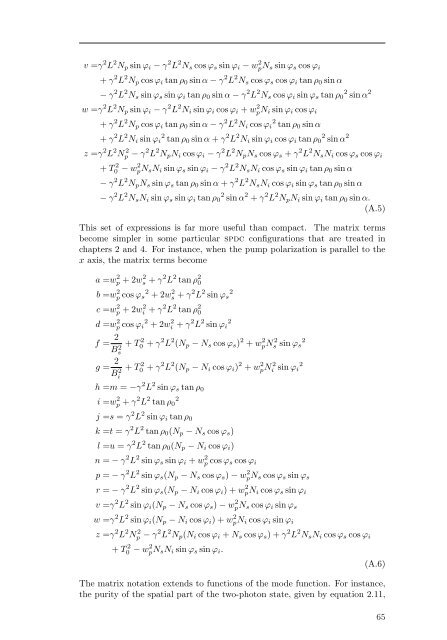
A. The matrix form of the mode function Each of the terms of the matrix is defined by comparing the product of the polynomial f with the argument of the exponential in equation 1.34. The elements of matrix A are a =w 2 p + 2w 2 s + γ 2 L 2 tan ρ 2 0 cos α 2 b =w 2 p cos ϕs 2 + 2w 2 s + γ 2 L 2 sin ϕs 2 − 2γ 2 L 2 sin ϕs cos ϕs sin α tan ρ0 + γ 2 L 2 cos ϕs 2 tan ρ0 2 sin α 2 c =w 2 p + 2w 2 i + γ 2 L 2 tan ρ 2 0 cos α 2 d =w 2 p cos ϕi 2 + 2w 2 i + γ 2 L 2 sin ϕi 2 + 2γ 2 L 2 sin ϕi cos ϕi tan ρ0 sin α + γ 2 L 2 cos ϕi 2 tan ρ0 2 sin α 2 f =2B −2 s + T 2 0 + γ 2 L 2 N 2 p + γ 2 L 2 N 2 s cos ϕs 2 + w 2 pN 2 s sin ϕs 2 − 2γ 2 L 2 NpNs cos ϕs − 2γ 2 L 2 NpNs sin ϕs tan ρ0 sin α + 2γ 2 L 2 N 2 s cos ϕs sin ϕs sin α tan ρ0 + γ 2 L 2 N 2 s sin ϕs 2 tan ρ0 2 sin α 2 g =2B −2 i + T 2 0 + γ 2 L 2 N 2 p + γ 2 L 2 N 2 i cos ϕi 2 + w 2 pN 2 i sin ϕi 2 − 2γ 2 L 2 NpNi cos ϕi + 2γ 2 L 2 NpNi sin ϕi tan ρ0 sin α − 2γ 2 L 2 N 2 i cos ϕi sin ϕi tan ρ0 sin α + γ 2 L 2 N 2 i sin ϕi 2 tan ρ0 2 sin α 2 h = − γ 2 L 2 sin ϕs tan ρ0 cos α + γ 2 L 2 cos ϕs tan ρ0 2 sin α cos α 2 i =w 2 p + γ 2 L 2 tan ρ0 2 cos α j =γ 2 L 2 sin ϕi tan ρ0 cos α + γ 2 L 2 cos ϕi tan ρ0 2 sin α cos α k =γ 2 L 2 Np tan ρ0 cos α − γ 2 L 2 Ns cos ϕs tan ρ0 cos α − γ 2 L 2 Ns sin ϕs tan ρ0 2 sin α cos α l =γ 2 L 2 Np tan ρ0 cos α − γ 2 L 2 Ni cos ϕi tan ρ0 cos α + γ 2 L 2 Ni sin ϕi tan ρ0 2 sin α cos α m = − γ 2 L 2 sin ϕs tan ρ0 cos α + γ 2 L 2 cos ϕs tan ρ0 2 sin α cos α n = − γ 2 L 2 sin ϕs sin ϕi + w 2 p cos ϕs cos ϕi + γ 2 L 2 cos ϕs sin ϕi sin α tan ρ0 − γ 2 L 2 sin ϕs cos ϕi sin α tan ρ0 + γ 2 L 2 cos ϕs cos ϕi tan ρ0 2 sin α 2 p = − γ 2 L 2 Np sin ϕs + γ 2 L 2 Ns cos ϕs sin ϕs − w 2 pNs cos ϕs sin ϕs + γ 2 L 2 Np cos ϕs tan ρ0 sin α − γ 2 L 2 Ns cos ϕs 2 tan ρ0 sin α + γ 2 L 2 Ns sin ϕs 2 tan ρ0 sin α − γ 2 L 2 Ns sin ϕs cos ϕs tan ρ0 2 sin α 2 r = − γ 2 L 2 Np sin ϕs + γ 2 L 2 Ni sin ϕs cos ϕi + w 2 pNi cos ϕs sin ϕi + γ 2 L 2 Np cos ϕs tan ρ0 sin α − γ 2 L 2 Ni cos ϕs cos ϕi tan ρ0 sin α − γ 2 L 2 Ni sin ϕs sin ϕi tan ρ0 sin α + γ 2 L 2 Ni cos ϕs sin ϕi tan ρ0 2 sin α 2 s =γ 2 L 2 sin ϕi tan ρ0 cos α + γ 2 L 2 cos ϕi tan ρ0 2 sin α cos α t =γ 2 L 2 Np tan ρ0 cos α − γ 2 L 2 Ns cos ϕs tan ρ0 cos α − γ 2 L 2 Ns sin ϕs tan ρ0 2 sin α cos α u =γ 2 L 2 Np tan ρ0 cos α − γ 2 L 2 Ni cos ϕi tan ρ0 cos α + γ 2 L 2 Ni sin ϕi tan ρ0 2 sin α cos α 64
v =γ 2 L 2 Np sin ϕi − γ 2 L 2 Ns cos ϕs sin ϕi − w 2 pNs sin ϕs cos ϕi + γ 2 L 2 Np cos ϕi tan ρ0 sin α − γ 2 L 2 Ns cos ϕs cos ϕi tan ρ0 sin α − γ 2 L 2 Ns sin ϕs sin ϕi tan ρ0 sin α − γ 2 L 2 Ns cos ϕi sin ϕs tan ρ0 2 sin α 2 w =γ 2 L 2 Np sin ϕi − γ 2 L 2 Ni sin ϕi cos ϕi + w 2 pNi sin ϕi cos ϕi + γ 2 L 2 Np cos ϕi tan ρ0 sin α − γ 2 L 2 Ni cos ϕi 2 tan ρ0 sin α + γ 2 L 2 Ni sin ϕi 2 tan ρ0 sin α + γ 2 L 2 Ni sin ϕi cos ϕi tan ρ0 2 sin α 2 z =γ 2 L 2 N 2 p − γ 2 L 2 NpNi cos ϕi − γ 2 L 2 NpNs cos ϕs + γ 2 L 2 NsNi cos ϕs cos ϕi + T 2 0 − w 2 pNsNi sin ϕs sin ϕi − γ 2 L 2 NsNi cos ϕs sin ϕi tan ρ0 sin α − γ 2 L 2 NpNs sin ϕs tan ρ0 sin α + γ 2 L 2 NsNi cos ϕi sin ϕs tan ρ0 sin α − γ 2 L 2 NsNi sin ϕs sin ϕi tan ρ0 2 sin α 2 + γ 2 L 2 NpNi sin ϕi tan ρ0 sin α. (A.5) This set of expressions is far more useful than compact. The matrix terms become simpler in some particular spdc configurations that are treated in chapters 2 and 4. For instance, when the pump polarization is parallel to the x axis, the matrix terms become a =w 2 p + 2w 2 s + γ 2 L 2 tan ρ 2 0 b =w 2 p cos ϕs 2 + 2w 2 s + γ 2 L 2 sin ϕs 2 c =w 2 p + 2w 2 i + γ 2 L 2 tan ρ 2 0 d =w 2 p cos ϕi 2 + 2w 2 i + γ 2 L 2 sin ϕi 2 f = 2 B2 s g = 2 B2 i + T 2 0 + γ 2 L 2 (Np − Ns cos ϕs) 2 + w 2 pN 2 s sin ϕs 2 + T 2 0 + γ 2 L 2 (Np − Ni cos ϕi) 2 + w 2 pN 2 i sin ϕi 2 h =m = −γ 2 L 2 sin ϕs tan ρ0 i =w 2 p + γ 2 L 2 tan ρ0 2 j =s = γ 2 L 2 sin ϕi tan ρ0 k =t = γ 2 L 2 tan ρ0(Np − Ns cos ϕs) l =u = γ 2 L 2 tan ρ0(Np − Ni cos ϕi) n = − γ 2 L 2 sin ϕs sin ϕi + w 2 p cos ϕs cos ϕi p = − γ 2 L 2 sin ϕs(Np − Ns cos ϕs) − w 2 pNs cos ϕs sin ϕs r = − γ 2 L 2 sin ϕs(Np − Ni cos ϕi) + w 2 pNi cos ϕs sin ϕi v =γ 2 L 2 sin ϕi(Np − Ns cos ϕs) − w 2 pNs cos ϕi sin ϕs w =γ 2 L 2 sin ϕi(Np − Ni cos ϕi) + w 2 pNi cos ϕi sin ϕi z =γ 2 L 2 N 2 p − γ 2 L 2 Np(Ni cos ϕi + Ns cos ϕs) + γ 2 L 2 NsNi cos ϕs cos ϕi + T 2 0 − w 2 pNsNi sin ϕs sin ϕi. (A.6) The matrix notation extends to functions of the mode function. For instance, the purity of the spatial part of the two-photon state, given by equation 2.11, 65
- Page 35 and 36: CHAPTER 2 Correlations and entangle
- Page 37 and 38: 2.1. The purity as a correlation in
- Page 39 and 40: 2.2. Correlations between space and
- Page 41 and 42: 2.2. Correlations between space and
- Page 43 and 44: 2.3. Correlations between signal an
- Page 45 and 46: 2.3. Correlations between signal an
- Page 47 and 48: Signal purity 1 0 (a) 0.1 3 2.3. Co
- Page 49 and 50: CHAPTER 3 Spatial correlations and
- Page 51 and 52: 3.2. OAM transfer in general SPDC c
- Page 53 and 54: 3.2. OAM transfer in general SPDC c
- Page 55: Phase front 3.3. OAM transfer in co
- Page 58 and 59: 4. OAM transfer in noncollinear con
- Page 60 and 61: 4. OAM transfer in noncollinear con
- Page 62 and 63: 4. OAM transfer in noncollinear con
- Page 64 and 65: 4. OAM transfer in noncollinear con
- Page 66 and 67: 4. OAM transfer in noncollinear con
- Page 68 and 69: 4. OAM transfer in noncollinear con
- Page 70 and 71: 4. OAM transfer in noncollinear con
- Page 72 and 73: 5. Spatial correlations in Raman tr
- Page 74 and 75: 5. Spatial correlations in Raman tr
- Page 76 and 77: 5. Spatial correlations in Raman tr
- Page 78 and 79: 5. Spatial correlations in Raman tr
- Page 81 and 82: CHAPTER 6 Summary This thesis chara
- Page 83: APPENDIX A The matrix form of the m
- Page 87: The matrix C is given by C = 1 ⎛
- Page 90 and 91: B. Integrals of the matrix mode fun
- Page 92 and 93: C. Methods for OAM measurements Inp
- Page 94 and 95: Bibliography [13] M. Barbieri, C. C
- Page 96 and 97: Bibliography [41] C. I. Osorio, A.
- Page 98: Bibliography [68] S. Chen, Y.-A. Ch
- Page 103: Spatial Characterization Of Two-Pho
- Page 107: A Luz Stella y Luis Alfonso, mis pa
- Page 110 and 111: Contents B Integrals of the matrix
- Page 112 and 113: When he [Kepler] found that his lon
- Page 114 and 115: Abstract The matrix notation, intro
- Page 116 and 117: Abstract La notación matricial int
- Page 118 and 119: Introduction the transfer of oam fr
- Page 121 and 122: CHAPTER 1 General description of Tw
- Page 123 and 124: y y x z z pump s i (a) signal idle
- Page 125 and 126: 1.3. Approximations and other consi
- Page 127 and 128: x 1.3. Approximations and other con
- Page 129 and 130: x Wave fronts 1.3. Approximations a
- Page 131 and 132: 1 0 -0.2 1.3. Approximations and ot
- Page 133: 1.4. The mode function in matrix fo
v =γ 2 L 2 Np sin ϕi − γ 2 L 2 Ns cos ϕs sin ϕi − w 2 pNs sin ϕs cos ϕi<br />
+ γ 2 L 2 Np cos ϕi tan ρ0 sin α − γ 2 L 2 Ns cos ϕs cos ϕi tan ρ0 sin α<br />
− γ 2 L 2 Ns sin ϕs sin ϕi tan ρ0 sin α − γ 2 L 2 Ns cos ϕi sin ϕs tan ρ0 2 sin α 2<br />
w =γ 2 L 2 Np sin ϕi − γ 2 L 2 Ni sin ϕi cos ϕi + w 2 pNi sin ϕi cos ϕi<br />
+ γ 2 L 2 Np cos ϕi tan ρ0 sin α − γ 2 L 2 Ni cos ϕi 2 tan ρ0 sin α<br />
+ γ 2 L 2 Ni sin ϕi 2 tan ρ0 sin α + γ 2 L 2 Ni sin ϕi cos ϕi tan ρ0 2 sin α 2<br />
z =γ 2 L 2 N 2 p − γ 2 L 2 NpNi cos ϕi − γ 2 L 2 NpNs cos ϕs + γ 2 L 2 NsNi cos ϕs cos ϕi<br />
+ T 2 0 − w 2 pNsNi sin ϕs sin ϕi − γ 2 L 2 NsNi cos ϕs sin ϕi tan ρ0 sin α<br />
− γ 2 L 2 NpNs sin ϕs tan ρ0 sin α + γ 2 L 2 NsNi cos ϕi sin ϕs tan ρ0 sin α<br />
− γ 2 L 2 NsNi sin ϕs sin ϕi tan ρ0 2 sin α 2 + γ 2 L 2 NpNi sin ϕi tan ρ0 sin α.<br />
(A.5)<br />
This set of expressions is far more useful than compact. The matrix terms<br />
become simpler in some particular spdc configurations that are treated in<br />
chapters 2 and 4. For instance, when the pump polarization is parallel to the<br />
x axis, the matrix terms become<br />
a =w 2 p + 2w 2 s + γ 2 L 2 tan ρ 2 0<br />
b =w 2 p cos ϕs 2 + 2w 2 s + γ 2 L 2 sin ϕs 2<br />
c =w 2 p + 2w 2 i + γ 2 L 2 tan ρ 2 0<br />
d =w 2 p cos ϕi 2 + 2w 2 i + γ 2 L 2 sin ϕi 2<br />
f = 2<br />
B2 s<br />
g = 2<br />
B2 i<br />
+ T 2 0 + γ 2 L 2 (Np − Ns cos ϕs) 2 + w 2 pN 2 s sin ϕs 2<br />
+ T 2 0 + γ 2 L 2 (Np − Ni cos ϕi) 2 + w 2 pN 2 i sin ϕi 2<br />
h =m = −γ 2 L 2 sin ϕs tan ρ0<br />
i =w 2 p + γ 2 L 2 tan ρ0 2<br />
j =s = γ 2 L 2 sin ϕi tan ρ0<br />
k =t = γ 2 L 2 tan ρ0(Np − Ns cos ϕs)<br />
l =u = γ 2 L 2 tan ρ0(Np − Ni cos ϕi)<br />
n = − γ 2 L 2 sin ϕs sin ϕi + w 2 p cos ϕs cos ϕi<br />
p = − γ 2 L 2 sin ϕs(Np − Ns cos ϕs) − w 2 pNs cos ϕs sin ϕs<br />
r = − γ 2 L 2 sin ϕs(Np − Ni cos ϕi) + w 2 pNi cos ϕs sin ϕi<br />
v =γ 2 L 2 sin ϕi(Np − Ns cos ϕs) − w 2 pNs cos ϕi sin ϕs<br />
w =γ 2 L 2 sin ϕi(Np − Ni cos ϕi) + w 2 pNi cos ϕi sin ϕi<br />
z =γ 2 L 2 N 2 p − γ 2 L 2 Np(Ni cos ϕi + Ns cos ϕs) + γ 2 L 2 NsNi cos ϕs cos ϕi<br />
+ T 2 0 − w 2 pNsNi sin ϕs sin ϕi.<br />
(A.6)<br />
The matrix notation extends to functions of the mode function. For instance,<br />
the purity of the spatial part of the two-photon state, given by equation 2.11,<br />
65


