Spatial Characterization Of Two-Photon States - GAP-Optique

1.0
0.0
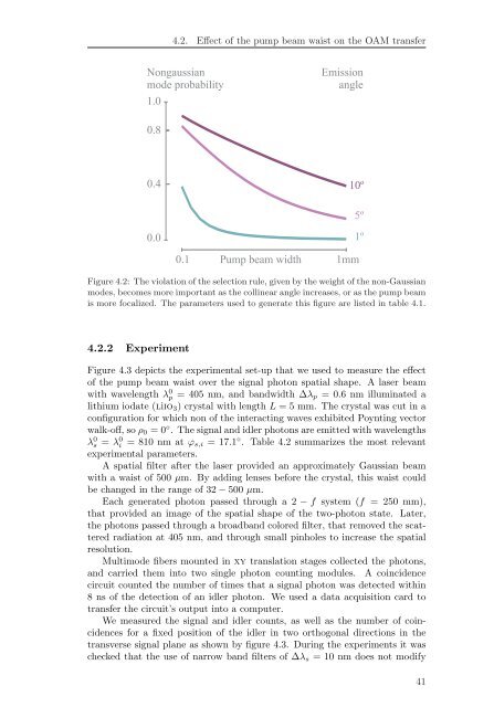
4.2. Effect of the pump beam waist on the OAM transfer
Nongaussian
mode probability
0.8
0.4
Emission
angle
10º
0.1 Pump beam width 1mm
Figure 4.2: The violation of the selection rule, given by the weight of the non-Gaussian
modes, becomes more important as the collinear angle increases, or as the pump beam
is more focalized. The parameters used to generate this figure are listed in table 4.1.
4.2.2 Experiment
Figure 4.3 depicts the experimental set-up that we used to measure the effect
of the pump beam waist over the signal photon spatial shape. A laser beam
with wavelength λ 0 p = 405 nm, and bandwidth ∆λp = 0.6 nm illuminated a
lithium iodate (liio3) crystal with length L = 5 mm. The crystal was cut in a
configuration for which non of the interacting waves exhibited Poynting vector
walk-off, so ρ0 = 0 ◦ . The signal and idler photons are emitted with wavelengths
λ 0 s = λ 0 i = 810 nm at ϕs,i = 17.1 ◦ . Table 4.2 summarizes the most relevant
experimental parameters.
A spatial filter after the laser provided an approximately Gaussian beam
with a waist of 500 µm. By adding lenses before the crystal, this waist could
be changed in the range of 32 − 500 µm.
Each generated photon passed through a 2 − f system (f = 250 mm),
that provided an image of the spatial shape of the two-photon state. Later,
the photons passed through a broadband colored filter, that removed the scattered
radiation at 405 nm, and through small pinholes to increase the spatial
resolution.
Multimode fibers mounted in xy translation stages collected the photons,
and carried them into two single photon counting modules. A coincidence
circuit counted the number of times that a signal photon was detected within
8 ns of the detection of an idler photon. We used a data acquisition card to
transfer the circuit’s output into a computer.
We measured the signal and idler counts, as well as the number of coincidences
for a fixed position of the idler in two orthogonal directions in the
transverse signal plane as shown by figure 4.3. During the experiments it was
checked that the use of narrow band filters of ∆λs = 10 nm does not modify
5º
1º
41