Spatial Characterization Of Two-Photon States - GAP-Optique
Spatial Characterization Of Two-Photon States - GAP-Optique
Spatial Characterization Of Two-Photon States - GAP-Optique

You also want an ePaper? Increase the reach of your titles
YUMPU automatically turns print PDFs into web optimized ePapers that Google loves.
5. <strong>Spatial</strong> correlations in Raman transitions<br />
Schmidt number<br />
40<br />
20<br />
1<br />
-180º<br />
0º 180º<br />
lenght spatial filter<br />
2 mm<br />
1 mm<br />
400 m<br />
200 m<br />
7<br />
4<br />
1<br />
-180º<br />
0º 180º<br />
100 m<br />
200 m<br />
500 m<br />
angle<br />
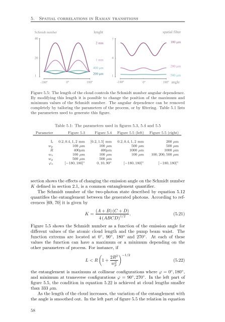
Figure 5.5: The length of the cloud controls the Schmidt number angular dependence.<br />
By modifying this length it is possible to change the position of the maximum and<br />
minimum values of the Schmidt number. The angular dependence can be removed<br />
completely by tailoring the parameters of the process, or by filtering. Table 5.1 lists<br />
the parameters used to generate this figure.<br />
Table 5.1: The parameters used in figures 5.3, 5.4 and 5.5<br />
Parameter Figure 5.3 Figure 5.4 Figure 5.5 (left) Figure 5.5 (right)<br />
L 0.2, 0.4, 1, 2 mm [0.2, 1.5] mm 0.2, 0.4, 1, 2 mm 200 µm<br />
wp 100 µm 100 µm 500 µm 500 µm<br />
R 400µm 400µm 1000 µm 1000 µm<br />
ws 100 µm 100 µm 100 µm 100, 200, 500 µm<br />
wg 500 µm 500 µm<br />
ϕs [−180, 180] ◦ 0, 10, 90 ◦ [−180, 180] ◦ [−180, 180] ◦<br />
section shows the effects of changing the emission angle on the Schmidt number<br />
K defined in section 2.1, is a common entanglement quantifier.<br />
The Schmidt number of the two-photon state described by equation 5.12<br />
quantifies the entanglement between the generated photons. According to references<br />
[69, 70] it is given by<br />
(A + B) (C + D)<br />
K =<br />
4 (ABCD) 1/2<br />
. (5.21)<br />
Figure 5.5 shows the Schmidt number as a function of the emission angle for<br />
different values of the atomic cloud length and the pump beam waist. The<br />
function extrema are located at 0 ◦ , 90 ◦ , 180 ◦ and 270 ◦ . At each of these<br />
values the function can have a maximum or a minimum depending on the<br />
other parameters of process. For instance, if<br />
L < R<br />
<br />
1 + 2R2<br />
w2 −1/2<br />
p<br />
(5.22)<br />
the entanglement is maximum at collinear configurations where ϕ = 0 ◦ , 180 ◦ ,<br />
and minimum at transverse configurations ϕ = 90 ◦ , 270 ◦ . In the left part of<br />
figure 5.5, the condition in equation 5.22 is achieved at cloud lengths smaller<br />
than 333 µm.<br />
As the length of the cloud increases, the variation of the entanglement with<br />
the angle is smoothed out. In the left part of figure 5.5 the relation in equation<br />
58