Spatial Characterization Of Two-Photon States - GAP-Optique

1. General description of two-photon states
In order to obtain more convenient units, the filter in momentum is defined
in a different way than the filter in frequency. While Bs,i → 0 implies a single
frequency collection, the condition for a single q vector collection is ws,i → ∞.
Finally, after all the approximations and taking into account the filters, the
mode function equation 1.12 becomes
Φ(qs, Ωs, qi, Ωi) ∝ exp − w2 p
4 ∆20 − w2 p
4 ∆21
× exp − (γL)2
4 ∆2k − T 2 0
4 (Ωs + Ωi) 2
× exp − w2 s
2 q2 s − w2 i
2 q2 i − 1
2B2 Ω
s
2 s − 1
2B2 Ω
i
2
i . (1.34)
The approximations listed in this chapter were introduced by several authors,
and can be found for example in references [39, 40, 30]. In reference [41],
we introduced a novel matrix notation based on the simplified mode function
equation 1.34. The next section explains the details and the advantages of that
notation.
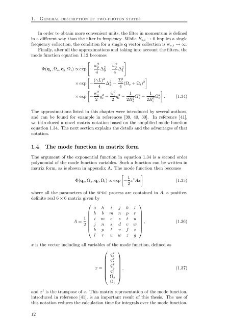
1.4 The mode function in matrix form
The argument of the exponential function in equation 1.34 is a second order
polynomial of the mode function variables. Such a function can be written in
matrix form, as is shown in appendix A. The mode function then becomes
Φ(qs, Ωs, qi, Ωi) ∝ exp − 1
2 xt
Ax
(1.35)
where all the parameters of the spdc process are contained in A, a positivedefinite
real 6 × 6 matrix given by
A = 1
⎛
a
⎜ h
⎜ i
2 ⎜ j
⎝ k
h
b
m
n
p
i
m
c
s
t
j
n
s
d
v
k
p
t
v
f
l
r
u
w
z
⎞
⎟ ,
⎟
⎠
(1.36)
l r u w z g
x is the vector including all variables of the mode function, defined as
⎛ ⎞
⎜
x = ⎜
⎝
q x s
q y s
q x i
q y
i
Ωs
Ωi
⎟ , (1.37)
⎟
⎠
and x t is the transpose of x. This matrix representation of the mode function,
introduced in reference [41], is an important result of this thesis. The use of
this notation reduces the calculation time for integrals over the mode function,
12