SHANNON SAMPLING SERIES WITH AVERAGED KERNELS1 1 ...

2 A.KIVUNUKK, G.TAMBERG
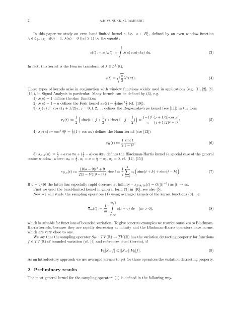
In this paper we study an even band-limited kernel s, i.e. s ∈ B 1 π, defined by an even window function
λ ∈ C [−1,1], λ(0) = 1, λ(u) = 0 (|u| 1) by the equality
s(t) := s(λ; t) :=
In fact, this kernel is the Fourier transform of λ ∈ L 1 (R),
s(t) =
1
0
λ(u) cos(πtu) du. (3)
π
2 λ∧ (πt). (4)
These types of kernels arise in conjunction with window functions widely used in applications (e.g. [1], [2], [8],
[16]), in Signal Analysis in particular. Many kernels can be defined by (3), e.g.
1) λ(u) = 1 defines the sinc function;
2) λ(u) = 1 − u defines the Fejér kernel sF (t) = 1 2 t
2sinc 2 (cf. [19]);
3) λj(u) := cos π(j + 1/2)u, j = 0, 1, 2, . . . defines the Rogosinski-type kernel (see [11]) in the form
2 πu
4) λH(u) := cos 2
rj(t) := 1
2
sinc(t + j + 1
1
) + sinc(t − j −
2 2 )
= (−1)j
π
1 = 2 (1 + cos πu) defines the Hann kernel (see [13])
(j + 1/2) cos πt
(j + 1/2) 2 ; (5)
− t2 sH(t) := 1 sinc t
; (6)
2 1 − t2 5) λB,a(u) := 1
1
2 + a cos πu + ( 2 − a) cos 3πu defines the Blackman-Harris kernel (a special case of the general
cosine window, where: a0 = 1
2 , a1 = a = 1
2 − a3, a2 = 0, cf. [14], [15])
sB,a(t) := (16a − 9)t2 + 9
2(1 − t 2 )(9 − t 2 )
sinc t = 1
2
3
k=0
ak
sinc(t + k) + sinc(t − k) . (7)
If a = 9/16 the latter has especially rapid decrease at infinity – s B,9/16(t) = O(|t| −5 ) as |t| → ∞.
First we used the band-limited kernel in general form (3) in [10], see also [5].
Now we will study the sampling operators (1) using averaged kernels of the kernel functions (3), i.e.
sm(t) := 1
m
m/2
−m/2
s(t + v) dv (m > 0), (8)
which is suitable for functions of bounded variation. To give concrete examples we restrict ourselves to Blackman-
Harris kernels, because they are rapidly decreasing at infinity and the Blackman-Harris operators have norms,
which are very close to one.
We say that the sampling operator SW : T V (R) → T V (R) has the variation detracting property for functions
f ∈ T V (R) of bounded variation (cf. [4] and references cited therein), if
VR[SW f] SW VR[f]. (9)
As an introductory approach we use averaged kernels to get for these operators the variation detracting property.
2. Preliminary results
The most general kernel for the sampling operators (1) is defined in the following way.