Documentation of the Evaluation of CALPUFF and Other Long ...

More documents

Recommendations

Info

FLEXPART 4 : The FLEXPART (Version 6.2; Siebert, 2006; Stohl et al., 2005 5 ) model is a Lagrangian particle dispersion model. FLEXPART was originally designed for calculating the long‐range and mesoscale dispersion of air pollutants from point sources, such as after an accident in a nuclear power plant. In the meantime FLEXPART has evolved into a comprehensive tool for atmospheric transport modeling and analysis CAMx 6 : The Comprehensive Air‐quality Model with extensions (CAMx; ENVIRON, 2010) is a photochemical grid model (PGM) that simulates inert or chemical reactive pollutants from the local to continental scale. As a grid model, it simulates transport and dispersion using finite difference techniques on a three‐dimensional array of grid cells. CALGRID: The California Mesoscale Photochemical Grid Model (Yamartino, et al., 1989, Scire et al., 1989; Earth Tech, 2005) is a PGM that simulates chemically reactive pollutants from the local to regional scale. CALGRID was originally designed to utilize meteorological fields produced by the CALMET meteorological processor (Scire et al., 2000a), but was updated in 2006 to utilize meteorology and emissions in UAM format (Earth Tech, 2006). The six LRT dispersion models represent two non‐steady‐state Gaussian puff models (CALPUFF and SCIPUFF), two three‐dimensional particle dispersion models (HYSPLIT and FLEXPART) and two three‐dimensional photochemical grid models (CAMx and CALGRID). HYSPLIT can also be run in a puff and hybrid particle/puff modes, which was investigated in sensitivity tests. All six LRT models were evaluated using the CAPTEX Release 3 and 5 field experiments and five of the six models (except CALGRID) were evaluated using the ETEX field experiment database. Evaluation Methodology Two different model performance evaluation methodologies were utilized in this study. The Irwin (1997) fitted Gaussian plume approach, as used in the EPA 1998 CALPUFF evaluation study (EPA, 1998a), was used for the same two tracer test field experiments used in the 1998 EPA study (i.e., GP80 and SRL75). This was done to elucidate how updates to CALPUFF model over the last decade have improved its performance. The second model evaluation approach adopts the spatial, temporal and global statistical evaluation framework of ATMES‐II (Mosca et. al., 1998; Draxler et al., 1998). The ATMES‐II uses statistical performance metrics of spatial, scatter, bias, correlation and cumulative distribution to describe model performance. An important finding of this study is that the fitted Gaussian plume model evaluation approach is very limited and can be a poor indicator of LRT dispersion model performance, with the ATMES‐ II approach providing a more comprehensive assessment of LRT model performance. Fitted Gaussian Plume Evaluation Approach The fitted Gaussian plume evaluation approach fits a Gaussian plume across the observed and predicted tracer concentrations along an arc of receptors at a specific downwind distance from the tracer release site. The approach focuses on a LRT dispersion model’s ability to replicate centerline concentrations and plume widths, modeled/observed plume centerline azimuth, plume arrival time, and plume transit time across the arc. We used the fitted Gaussian plume evaluation approach to evaluate CALPUFF for the GP80 and SRL75 tracer experiments where the tracer concentrations were observed along arcs of receptors, as was done in the EPA 1998 CALPUFF evaluation study (EPA, 1998a). 4 http://transport.nilu.no/flexpart 5 http://www.atmos‐chem‐phys.net/5/2461/2005/acp‐5‐2461‐2005.html 6 http://www.camx.com/ 4
CALPUFF performance is evaluated by calculating the predicted and observed cross‐wind integrated concentration (CWIC), azimuth of plume centerline, and the second moment of tracer concentration (lateral dispersion of the plume [σy]). The CWIC is calculated by trapezoidal integration across average monitor concentrations along the arc. By assuming a Gaussian distribution of concentrations along the arc, a fitted plume centerline concentration (Cmax) can be calculated by the following equation: Cmax = CWIC/[(2π) ½ σy] The measure σy describes the extent of plume horizontal dispersion. This is important to understanding differences between the various dispersion options available in the CALPUFF modeling system. 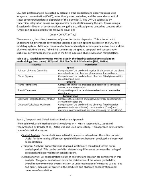Additional measures for temporal analysis include plume arrival time and the plume transit time on arc. Table ES‐1 summarizes the spatial, temporal and concentration statistical performance metrics used in the fitted Gaussian plume evaluation methodology. Table ES‐1. Model performance metrics used in the fitted Gaussian plume evaluation methodology from Irwin (1997) and 1998 EPA CALPUFF Evaluation (EPA, 1998a). Statistics Description Spatial Azimuth of Plume Centerline Comparison of the predicted angular displacement of the plume centerline from the observed plume centerline on the arc Plume Sigma‐y Comparison of the predicted and observed fitted plume widths (i.e., dispersion rate) Temporal Plume Arrival Time Compare the time the predicted and observed tracer clouds arrives on the receptor arc Transit Time on Arc Compare the predicted and observed residence time on the receptor arc Concentration Crosswind Integrated Concentration Compares the predicted and observed average concentrations across the receptor arc Observed/Calculated Maximum Comparison of the predicted and observed fitted Gaussian plume centerline (maximum) concentrations (Cmax) and maximum concentration at any receptor along the arc (Omax) Spatial, Temporal and Global Statistics Evaluation Approach The model evaluation methodology as employed in ATMES‐II (Mosca et al., 1998) and recommended by Draxler et al., (2002) was also used in this study. This approach defines three types of statistical analyses: • Spatial Analysis: Concentrations at a fixed time are considered over the entire domain. Useful for determining differences spatial differences between predicted and observed concentrations. • Temporal Analysis: Concentrations at a fixed location are considered for the entire analysis period. This can be useful for determining differences between the timing of predicted and observed tracer concentrations. • Global Analysis: All concentration values at any time and location are considered in this analysis. The global analysis considers the distribution of the values (probability), overall tendency towards overestimation or underestimation of measured values (bias and error), measures of scatter in the predicted and observed concentrations and measures of correlation. 5
Page 1 and 2: Documentation of the Evaluation of
Page 3 and 4: FOREWARD This report documents the
Page 5 and 6: 2.4.3 ATMES‐II Model Evaluation A
Page 7 and 8: EXECUTIVE SUMMARY ABSTRACT The CALP
Page 9: OVERVIEW OF APPROACH Up to six LRT
Page 13 and 14: Table ES‐2. ATMES‐II spatial an
Page 15 and 16: • CALPUFF tended to overstate the
Page 17 and 18: • The best performing CALPUFF con
Page 19 and 20: 2009a). The key findings from the C
Page 21 and 22: 1.8 1.6 1.4 1.2 1.0 0.8 0.6 0.4 0.2
Page 23 and 24: 2.4 2 1.6 1.2 0.8 0.4 0 EXP4A EXP4B
Page 25 and 26: Figure ESS‐4. RANK statistical pe
Page 27 and 28: Evaluatioon of Six LRT T Dispersion
Page 29 and 30: Table ES‐6. Summary of model rank
Page 31 and 32: eproduce the northwest to southeast
Page 33 and 34: ETEX LRT Dispersion Model Sensitivi
Page 35 and 36: CONCLUSIONS OF LRT DISPERSION MODEL
Page 37 and 38: The CAMx and CALGRID Eulerian photo
Page 39 and 40: July 1980. Both experiments examine
Page 41 and 42: 1.3 ORGANIZATION OF REPORT Chapter
Page 43 and 44: puffs expand until they exceed the
Page 45 and 46: that performance evaluation be base
Page 47 and 48: The ETEX real‐time LRT modeling p
Page 49 and 50: The ETEX study has formulated the f
Page 51 and 52: In this study we expand the LRT mod
Page 53 and 54: AM ∩ AP FMS = × 100% (2‐2) A
Page 55 and 56: Factor of α (FAα): FAα represent
Page 57 and 58: 3.0 1980 GREAT PLAINS FIELD STUDY 3
Page 59 and 60: compact discs, which were used to o
Page 61 and 62:
ILEVZI = 1 Layer of winds to use in
Page 63 and 64:
MCHEM = 0 No chemical transformatio
Page 65 and 66:
Table 3‐6. CALPUFF/CALMET experim
Page 67 and 68:
Table 3‐11. CALPUFF/MMIF sensitiv
Page 69 and 70:
evaluation studies and evaluate whe
Page 71 and 72:
Tables 3‐13 and Figures 3‐2 thr
Page 73 and 74:
140% 120% 100% 80% 60% 40% 20% 0%
Page 75 and 76:
30% 20% 10% 0% ‐10% ‐20% ‐30%
Page 77 and 78:
120% 100% 80% 60% 40% 20% 0% ‐20%
Page 79 and 80:
20% 10% 0% ‐10% ‐20% ‐30% ‐
Page 81 and 82:
The fitted Gaussian plume statistic
Page 83 and 84:
0% ‐10% ‐20% ‐30% ‐40% ‐5
Page 85 and 86:
300% 250% 200% 150% 100% 50% 0% 300
Page 87 and 88:
60% 40% 20% 0% ‐20% ‐40% ‐60%
Page 89 and 90:
with APS, implementing the slug opt
Page 91 and 92:
the amount of time that the tracer
Page 93 and 94:
Figure 4‐1. CALPUFF/CALMET UTM mo
Page 95 and 96:
compact discs, which were used to o
Page 97 and 98:
Table 4‐4. CALPUFF parameters use
Page 99 and 100:
Table 4‐8. CALPUFF/MMIF sensitivi
Page 101 and 102:
the fitted Gaussian plume is not a
Page 103 and 104:
Figure 4‐2. Comparison of predict
Page 105 and 106:
Figure 5‐1. Location of Dayton an
Page 107 and 108:
MM5 runs, the first without FDDA (i
Page 109 and 110:
Table 5‐3. MM5 sensitivity tests
Page 111 and 112:
Table 5‐6. Definition of the CALM
Page 113 and 114:
performance at the monitor location
Page 115 and 116:
35% 30% 25% 20% 15% 10% 5% 0% 35% 3
Page 117 and 118:
40% 35% 30% 25% 20% 15% 10% 5% 0% F
Page 119 and 120:
40% 35% 30% 25% 20% 15% 10% 5% 0% E
Page 121 and 122:
5.4.1.4 Comparison of CALPUFF CTEX3
Page 123 and 124:
0.48 0.36 0.24 0.12 0 ‐0.12 16% 1
Page 125 and 126:
CTEX3 discussed in Section 5.4.1. A
Page 127 and 128:
CALPUFF sensitivity simulations are
Page 129 and 130:
14. Across all the spatial statisti
Page 131 and 132:
sensitivity tests. The “B” seri
Page 133 and 134:
‐0.1 ‐0.2 0 0.8 0.7 0.6 0.5 0.4
Page 135 and 136:
6.0 1994 EUROPEAN TRACER EXPERIMENT
Page 137 and 138:
Figure 6‐2a. Surface synoptic met
Page 139 and 140:
Figure 6‐3a. Distribution of the
Page 141 and 142:
36 kilometers and the vertical stru
Page 143 and 144:
splitting flag near sunset (hour 17
Page 145 and 146:
experienced during the original ETE
Page 147 and 148:
2 1 0 ‐1 ‐2 3 2 1 0 23‐Oct 23
Page 149 and 150:
70% 60% 50% 40% 30% 20% 10% 0% Figu
Page 151 and 152:
Figure 6‐9. Factor of Exceedance
Page 153 and 154:
eceiving a 0.0 score. Figure 6‐13
Page 155 and 156:
Table 6‐1. Summary of model ranki
Page 157 and 158:
plume spread and observed surface c
Page 159 and 160:
Figure 6‐16c. Comparison of spati
Page 161 and 162:
• NoPiG: The tracer emissions wer
Page 163 and 164:
Using the NMSE statistical performa
Page 165 and 166:
6.4.3.2 Effect of PiG on Model Perf
Page 167 and 168:
80 70 60 50 40 30 20 10 0 1 2 3 4 5
Page 169 and 170:
Table 6‐3. Summary of CALPUFF puf
Page 171 and 172:
0.2 0.18 0.16 0.14 0.12 0.1 0.08 0.
Page 173 and 174:
Figure 6‐ ‐22 displays the t sp
Page 175 and 176:
Figure 6‐ ‐23a. Global model pe
Page 177 and 178:
Figure 6‐24. Figure of Merit (FMS
Page 179 and 180:
7.0 REFERENCES Anderson, B. 2008. T
Page 181 and 182:
EPA, 1984: Interim Procedures for E
Page 183 and 184:
Mlawer, E.J., S.J. Taubman, P.D. Br
Page 185 and 186:
148 Appendix A Evaluation of the MM
Page 187 and 188:
Table A‐1. Wind speed and wind di
Page 189 and 190:
Table A‐3. Definition of the CTEX
Page 191 and 192:
Figure A‐ ‐1. Wind speed bias (
Page 193 and 194:
Figure A‐ ‐3. Humidity bias and
Page 195 and 196:
Table A‐5. Comparison of CTEX5 MM
Page 197 and 198:
B.1 CALMET MODEL EVALUATION TO IDEN
Page 199 and 200:
Figure B‐ ‐1 displays th he win
Page 201 and 202:
Table B‐2a. Summary wind speed mo
Page 203 and 204:
B.2 CONCLUSIONS OF CTEX3 CALMET SEN
Page 205 and 206:
C.1 INTRODUCTION In this section, t
Page 207 and 208:
C.2.2 HYYSPLIT GLOB BAL STATISTIICS
Page 209 and 210:
The final panel in Figure C‐3 (bo
Page 211 and 212:
Figure C‐ ‐5. Global model m pe
Page 213 and 214:
C.3 CAMX SENSITIVITY TESTS Followin
Page 215 and 216:
ACM2 Kzz combinatio ons rank as the
Page 217 and 218:
Figure C‐ ‐10. Spatial model pe
Page 219 and 220:
Figure C‐ ‐12. Global model per
Page 221 and 222:
Figure C‐ ‐13. Spatial model pe
Page 223 and 224:
Page 225 and 226:
Page 227 and 228:
Table C‐3. CAMx FMS and POD spati
Page 229 and 230:
Figure C‐ ‐20. False Alarm Rate
Page 231 and 232:
Figure C‐ ‐23. Factor of o Exce
Page 233 and 234:
The PCC values for th he six LRT mo
Page 235 and 236:
The RANK statistical performancce m
Page 237 and 238:
Table C‐55. Summary y of model r
Page 239 and 240:
Results foor the TS me etric are pr
Page 241 and 242:
Figure C‐ ‐35. Factor of o 2 (F
Page 243 and 244:
a negativve FB. The best b performm
Page 245 and 246:
performing model the most often sco
Page 247:
United States Environmental Protect
show all

Documentation of the Evaluation of CALPUFF and Other Long ...

Create successful ePaper yourself

Delete template?

Save as template?