The.Algorithm.Design.Manual.Springer-Verlag.1998

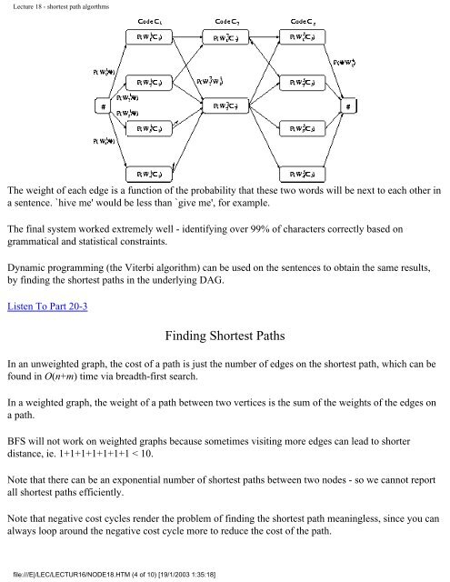
Lecture 18 - shortest path algorthms
The weight of each edge is a function of the probability that these two words will be next to each other in
a sentence. `hive me' would be less than `give me', for example.
The final system worked extremely well - identifying over 99% of characters correctly based on
grammatical and statistical constraints.
Dynamic programming (the Viterbi algorithm) can be used on the sentences to obtain the same results,
by finding the shortest paths in the underlying DAG.
Listen To Part 20-3
Finding Shortest Paths
In an unweighted graph, the cost of a path is just the number of edges on the shortest path, which can be
found in O(n+m) time via breadth-first search.
In a weighted graph, the weight of a path between two vertices is the sum of the weights of the edges on
a path.
BFS will not work on weighted graphs because sometimes visiting more edges can lead to shorter
distance, ie. 1+1+1+1+1+1+1 < 10.
Note that there can be an exponential number of shortest paths between two nodes - so we cannot report
all shortest paths efficiently.
Note that negative cost cycles render the problem of finding the shortest path meaningless, since you can
always loop around the negative cost cycle more to reduce the cost of the path.
file:///E|/LEC/LECTUR16/NODE18.HTM (4 of 10) [19/1/2003 1:35:18]