THE ANALYSIS OF CATEGORICAL DATA: FISHER'S EXACT TEST

THE ANALYSIS OF
CATEGORICAL DATA:
FISHER’S EXACT TEST
Jenny V Freeman and Michael J Campbell
analyse categorical data in small samples
IN THE PREVIOUS TUTORIAL we have
outlined some simple methods for
analysing binary data, including the
comparison of two proportions using
the Normal approximation to the
binomial and the Chi-squared test. 1
However, these methods are only
approximations, although they are
good when the sample size is large.
When the sample size is small we can
evaluate all possible combinations of
the data and compute what are known
as exact P-values.
FISHER’S EXACT TEST
When one of the expected values (note:
not the observed values) in a 2 × 2 table
is less than 5, and especially when it is
less than 1, then Yates’ correction can
be improved upon. In this case Fisher’s
Exact test, proposed in the mid-1930s
almost simultaneously by Fisher, Irwin
and Yates, 2
can be applied. The null
hypothesis for the test is that there is
no association between the rows and
columns of the 2 × 2 table, such that
the probability of a subject being in a
particular row is not influenced by
being in a particular column. If the
columns represent the study group
and the rows represent the outcome,
then the null hypothesis could be
interpreted as the probability of having
a particular outcome not being
influenced by the study group, and the
test evaluates whether the two study
groups differ in the proportions with
each outcome.
An important assumption for all of
the methods outlined, including
Fisher’s Exact test, is that the binary
data are independent. If the
proportions are correlated then more
advanced techniques should be
applied. For instance in the leg ulcer
example of the previous tutorial, 1 if
there were more than one leg ulcer per
patient, we could not treat the
outcomes as independent.
The test is based upon calculating
directly the probability of obtaining the
results that we have shown (or results
more extreme) if the null hypothesis is
actually true, using all possible 2 × 2
tables that could have been observed,
for the same row and column totals as
the observed data. These row and
column totals are also known as
marginal totals. What we are trying to
establish is how extreme our particular
table (combination of cell frequencies)
is in relation to all the possible ones
that could have occurred given the
marginal totals.
This is best explained by a simple
worked example. The data in table 1
come from an RCT comparing intramuscular
magnesium injections with
placebo for the treatment of chronic
fatigue syndrome. 3 Of the 15 patients
who had the intra-muscular
magnesium injections 12 felt better (80
per cent) whereas, of the 17 on placebo,
only three felt better (18 per cent).
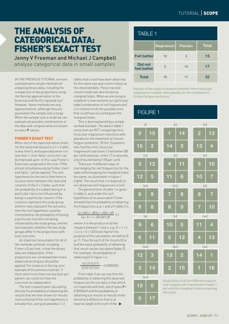
There are 16 different ways of
rearranging the cell frequencies for the
table whilst keeping the marginal totals
the same, as illustrated in figure 1
(right). The result that corresponds to
our observed cell frequencies is (xiii).
The general form of table 1 is given
in table 2, and under the null
hypothesis of no association Fisher
showed that the probability of obtaining
the frequencies a, b, c and d in table 2 is
(a + b)!(c + d)!(a + c)!(b + d)!
(1)
(a + b + c + d)!a!b!c!d!
where x! is the product of all the
integers between 1 and x, e.g. 5! = 1 × 2
× 3 × 4 × 5 = 120 (note that for the
purpose of this calculation, we define 0!
as 1). Thus for each of the results (i) to
(xvi) the exact probability of obtaining
that result can be calculated (table 3).
For example, the probability of
obtaining (i) in figure 1 is
15!17!15!17!
= 0.0000002.
32!0!15!15!2!
From table 3 we can see that the
probability of obtaining the observed
frequencies for our data is that which
corresponds with (xiii), which gives P =
0.0005469 and the probability of
obtaining our results or results more
extreme (a difference that is at
least as large) is the sum of the
▼
TABLE 1
FIGURE 1
TUTORIAL | SCOPE
Total
Felt better 12 3 15
Did not
feel better
Magnesium Placebo
3 14 17
Total 15 17 32
Results of the study to examine whether intra-muscular
magnesium is better than placebo for the treatment of
chronic fatigue syndrome. †
(i) (ii) (iii)
0 15
15 2
3 12
12 5
1 14
14 3
4 11
11 6
2 13
13 4
(iv) (v) (vi)
6 9
9 8
7 8
8 9
5 10
10 7
(vii) (viii) (ix)
9 6
6 11
10 5
5 12
8 7
7 10
(x) (xi) (xii)
12 3
3 14
13 2
2 15
11 4
4 13
(xiii) (xiv) (xv)
(xvi)
15 0
0 17
14 1
1 16
Illustration of all the different ways of
rearranging cell frequencies in table 1,
but with the marginal totals remaining
the same.
SCOPE | JUNE 07 | 11

▼
SCOPE | TUTORIAL
TABLE 2
General form of table 1.
Probabilities of each of the frequency tables above,
calculated using formula 1.
12 | JUNE 07 | SCOPE
Total
Row 1 a b a + b
Row 2 c d c + d
Total a + b b + d
TABLE 3
Column 1 Column 2
a + b +
c + d
Total a b c d P-value
i 0 15 15 2 0.0000002
ii 1 14 14 3 0.0000180
iii 2 13 13 4 0.0004417
iv 3 12 12 5 0.0049769
v 4 11 11 6 0.0298613
vi 5 10 10 7 0.1032349
vii 6 9 9 8 0.2150728
viii 7 8 8 9 0.2765221
ix 8 7 7 10 0.2212177
x 9 6 6 11 0.1094916
xi 10 5 5 12 0.0328475
xii 11 4 4 13 0.0057426
xiii 12 3 3 14 0.0005469
xiv 13 2 2 15 0.0000252
xv 14 1 1 16 0.0000005
xvi 15 0 0 17 0.0000000
TABLE 4
Treatment
Outcome Total
Clinic Home
Healed 22 (18%) 17 (15%) 39
Not healed 98 (82%) 77 (85%) 194
Total 120 (100%) 113 (100%) 233
2 × 2 contingency table of treatment (clinic/home) by
outcome (ulcer healed/not healed) for the leg ulcer study.
probabilities for (xiii) to (xvi) = 0.000573.
This gives the one-sided P-value for
obtaining our results or results more
extreme, and in order to obtain the twosided
P-value there are several
approaches. The first is to simply
double this value, which gives P =
0.0001146. A second approach is to add
together all the probabilities that are
the same size or smaller than the one
for our particular result; in this case,
all probabilities that are less than or
equal to 0.0005469, which are (i), (ii),
(iii), (xiii), (xiv), (xv) and (xvi). This gives a
two-sided value of P = 0.001033.
Generally the difference is not great,
though the first approach will always
give a value greater than the second. A
third approach, which is recommended
by Swinscow and Campbell, 4 is a
compromise and is known as the mid-P
method. All the values more extreme
than the observed P-value are added
up and these are added to one half of
the observed value. This gives P =
0.000759.
COMPARISON OF TESTS
The criticism of the first two methods is
that they are too conservative, i.e. if the
null hypothesis was true, over repeated
studies they would reject the null
hypothesis less often than 5 per cent.
They are conditional on both sets of
marginal totals being fixed, i.e. exactly
15 people being treated with
magnesium and 15 feeling better. However
if the study were repeated, even
with 15 and 17 in the magnesium and
placebo groups respectively, we would
not necessarily expect exactly 15 to feel
better. The mid-P value method is less
conservative, and gives approximately
the correct rate of type I errors (false
positives).
In either case, for our example, the
P-value is less than 0.05, the nominal
level for statistical significance and we
can conclude that there is evidence of a
statistically significant difference in the
proportions feeling better between the
two treatment groups. However, in
common with other non-parametric
tests, Fisher’s Exact test is simply a
hypothesis test. It will merely tell you
whether a difference is likely, given the
null hypothesis (of no difference). It
gives you no information about the
likely size of the difference, and so
whilst we can conclude that there is a
significant difference between the two
treatments with respect to feeling
better or not, we can draw no
conclusions about the possible size of
the difference.
EXAMPLE DATA
FROM LAST WEEK
Table 4 shows the data from the
previous tutorial. It is from a
randomised controlled trial of
community leg ulcer clinics, 5 comparing
the cost effectiveness of community leg
ulcer clinics with standard nursing
care. The columns represent the two
treatment groups, specialist leg ulcer
clinic (clinic) and standard care (home),
and the rows represent the outcome
variable, in this case whether the leg
ulcer has healed or not.
For this example the two-sided Pvalue
from Fisher’s Exact test is 0.599
and in this case we cannot reject the
null hypothesis and would decide that
there is a insufficient evidence to a
difference between the two groups.
SUMMARY
This tutorial has described in detail
Fisher’s Exact test, for analysing simple
2 × 2 contingency tables when the
assumptions for the Chi-squared test
are not met. It is tedious to do by hand,
but nowadays is easily computed by
most statistical packages.
† When organising data such as this is it good
practice to arrange the table with the grouping
variable forming the columns and the outcome
variable forming the rows.
REFERENCES
1 Freeman JV, Julious SA. The
analysis of categorical data.
Scope 2007; 16(1): 18–21.
2 Armitage P, Berry PJ,
Matthews JNS. Statistical
methods in medical
research. 4th ed. Oxford:
Blackwell Publishing, 2002.
3 Cox IM, Campbell MJ,
Dowson D. Red blood cell
magnesium and chronic
fatigue syndrome. Lancet
1991; 337: 757–60.
4 Swinscow TDV, Campbell
MJ. Statistics at square one.
10th ed. London: BMJ
Books, 2002.
5 Morrell CJ, Walters SJ,
Dixon S, Collins K, Brereton
LML, Peters J et al. Cost
effectiveness of community
leg ulcer clinic: randomised
controlled trial. Brit Med J
1998; 316: 1487–91.