Continuous and discontinuous variation - BiologyMad A-Level Biology

Continuous and discontinuous variation
Variation, the small differences that exist between individuals, can be described as being either
discontinuous or continuous.
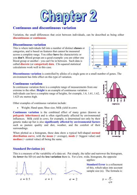
Discontinuous variation
This is where individuals fall into a number of distinct classes or
categories, and is based on features that cannot be measured
across a complete range. You either have the characteristic or
you don't. Blood groups are a good example: you are either one
blood group or another - you can't be in between. Such data is
called discrete (or categorical) data. Chi-squared statistical
calculations work well in this case.
Discontinuous variation is controlled by alleles of a single gene or a small number of genes. The
environment has little effect on this type of variation.
Continuous variation
In continuous variation there is a complete range of measurements from one
extreme to the other. Height is an example of continuous variation -
individuals can have a complete range of heights, for example, 1.6, 1.61, 1.62,
1.625 etc metres high.
Other examples of continuous variation include:
• Weight; Hand span; Shoe size; Milk yield in cows
Continuous variation is the combined effect of many genes (known as
polygenic inheritance) and is often significantly affected by environmental
influences. Milk yield in cows, for example, is determined not only by their
genetic make-up but is also significantly affected by environmental factors
such as pasture quality and diet, weather, and the comfort of their
surroundings.
When plotted as a histogram, these data show a typical bell-shaped normal
distribution curve, with the mean (= average), mode (= biggest value) and
median (= central value) all being the same.
Standard Deviation (σ)
This is a measure of the variability of a data set. Put simply, the taller and narrower the histogram,
the lower the SD (σ) and the less variation there is. For a low, wide, histogram, the opposite
applies:
Standard Error is a refinement
of this, which takes into account
sample size (n). The formula is:

Sampling Error
When collecting data, it is vital that the data is reliable and reflects real differences in the
population. This can be ensured by having a large data size, but it is also necessary to ensure that
the data collected is typical of the whole population – in other words, that it is randomly
collected. In the laboratory, we repeat experiments 3 times and/or pool class data. In field-work,
we use random number tables; grids laid out with tape-measures, and large numbers of quadrats
to ensure that our data are reliable and randomly collected.
N.B. It is easy to (unwittingly) introduce bias into the collection of results, and ‘to avoid bias’ is an
important point to make in your answers to questions on this topic
Causes of Variation
Variation in the phenotype is caused either by the environment, by genetics, or by a combination of
the two. Meiosis and sexual reproduction introduces variation (see Ch 1), through Independent
assortment of the parental chromosomes; through Crossing-over during Prophase I; and through
the random fertilisation that forms the zygote.
Mutations
These changes to the genetic make-up of an individual which
cannot be accounted for by the normal processes (above)
may (rarely) involve chromosomal mutations (e.g. Down’s
Syndrome, where an individual has trisomy (= 3 copies) of
chromosome 21; they therefore have 47 chromosomes), but
more commonly, these mutations are confined to a single
gene and are known as gene mutations. Since DNA
replication is not perfect, with an error rate of about 1 in 10 12 bases, we gradually acquire more of
these during our lives. Certain chemicals and radiation increase this error rate, but note that 99% of
our DNA is ‘junk DNA’ and so the vast majority of mutations are unlikely to have any effect
whatsoever.
Base deletion means a single base is omitted. This will affect all subsequent amino-acids in that
protein and the effects are therefore likely to be severe.
Gene pool
Base substitution means that one base is replaced by another. This will only
affect a single amino-acid, and normally this has little effect unless the active
site of an enzyme is affected. One example where the effects are dramatic is
sickle-cell anaemia, which is caused by a single amino-acid substitution (see
later notes)
This is the total number of alleles (note, not genes!) in a breeding
population. A human population will have 3 alleles for blood
groups (A, B, O). Since everyone must have one of each of these
alleles, the total frequency must be 1.0 and the frequency of each
allele can then be expressed as a decimal. In the above case, the
frequencies vary greatly amongst different ethnic groups (see
table)
Population I A I B
I O
African 15 10 75
Caucasian 30 15 55
Orientals 20 22 58
Amer. Indians 0-55 0 45-100
Australasian 50 0 50
Worldwide 22 16 62
Europe 22 11 67

•
•
•
•
•
Hardy – Weinberg
This principle states that the proportion of the different alleles in a gene
pool (breeding population) only changes as a result of an external factor.
Thus providing the following assumptions are met, each generation will
be the same as the present one:
Large population
No migration – either in (immigration) or out (emigration)
There is random mating
No mutations occur
All genotypes are equally fertile
Worked Example:
In a population containing 2 alleles, T and t, three genotypes
will exist – TT, Tt and tt. If T is a dominant allele, then it is
impossible to tell which individuals are Tt and which are Tt. It
will also be impossible to tell the relative proportions of these
two genotypes. The Hardy-Weinberg equation allows us to
calculate that.
Stages in the calculation:
Let the proportion of T alleles = p and the proportion of t alleles
= q. Then:
p + q = 1
Both p and q are decimal fractions, and therefore both will be
less than 1.0.
That means that the proportion of the different genotypes is:
TT individuals are p 2 ;
Tt individuals are 2 pq; and
Tt individuals are q 2
Since that is the whole population, it follows that:
1 = p 2 + 2pq + q 2
Now, we can see, and count, those individuals that are tt
(double recessive), so:
1. Work out the proportion (as a decimal fraction, i.e.
5% = 0.05) of tt individuals in the whole population.
The question will give you this data, so just use your
calculator!
2. Take the square root of that number. That gives you q
3. Since p + q = 1, you can now calculate p (it is 1 − q).
4. Substitute the values you now have in the equation 1 =
p 2 + 2pq + q 2 to give you the decimal fraction of each
of the genotypes.
5. If the question asks you to calculate ‘how many individuals in then population are….’,
then multiply the number you have (for the required genotype) by the total population.
Remember that you cannot have a fraction of an individual, so round up/down to the
nearest whole number.
6. Easy, isn’t it!

Natural selection
The Hardy-Weinberg equation requires such stringent
conditions to be met, that, in the real world, it is seldom, if
ever, true. Thus, the equation is used to show that
populations change over time, something we normally call
evolution.
The driving force behind evolution is natural selection, and
this can occur in three main ways:
Stabilising selection:
This is the most common, and is a response to a stable
environment. A good example is birth weight, since underweight
babies are clearly less likely to survive, and overweight
babies are likely to get stuck during birth, killing not
only themselves, but also their mothers! The result is that
the mode stays the same, but the SD of the population
falls, i.e. the population graph gets narrower and taller, as
selection against mutations takes place. This is most
apparent in small, isolated populations, or when a bottleneck
event takes place.
Directional selection:
A bottleneck event occurs when a population is reduced to
just a few breeding individuals (e.g. cheetahs). Though the
total population may later recover, they will all be
descendants of the few originals (Adam and Eve?) and so
will have a much narrower gene pool than the original
population.
There have been a number of events in geological history
(‘mass extinctions’) when all forms of life on Earth were
reduced to around 1% of the previous community. These
events are followed by rapid evolution and an increase
in diversity, as species evolve to fill every available niche.
The last such event was 65 million years ago, when the
Dinosaurs became extinct, allowing mammals to replace
reptiles as the dominant life-forms on Earth.
This is the most common form of selection that results in a population with
a new trait. It takes place whenever change occurs in the environment,
such as when a poison is used and resistant
individuals begin to occur. These soon
become the dominant type within the
population. It does not matter if the
example is Warfarin resistance in rats,
DDT resistance in mosquitoes, or antibiotic
resistance in bacteria. In Nature, such
selection can also occur, as we saw, in
spine selection in Holly, or when cacti are
grazed (see left):

Disruptive selection:
This is much less common and results in two distinct
populations, or morphs. Eventually, these two forms
may become so distinct that they become new
populations.
The example usually used is Biston betularia,
the Peppered Moth (left). This moth hides
on birch-trees during the day, and two forms
are favoured – like (clean air, pale tree-trunks)
and dark (sooty air, dark tree-trunks). Any
intermediate forms are obvious on any tree,
and so are selected against. The dark (or
melanic) form became more common in
polluted city air after the Industrial
Revolution, but has now become rare again,
following the Clean Air Acts of the last 50
years. This is usually used as an example of
Natural Selection in action.
Sickle-Cell Anaemia
Sickle-cell is an inherited condition in which two co-dominant alleles exist – Hb S and Hb A . This
condition is caused by a single point substitution mutation, resulting in a single amino-acid being
changed. With 2 alleles, three phenotypes therefore exist:
1.
2.
3.
Hb S Hb S . These individuals have sickle-cell anaemia, and normally
die young.
Hb S Hb A . These individuals have sickle-cell trait, have only a few
sickle-cells and are resistant to malaria
Hb A Hb A . These individuals are normal, and are susceptible to
malaria.
In most parts of the world, stabilising selection selects against this mutation,
so it is very rare. However, in parts of the world where malaria is
common, there is a selective advantage in having sickle-cell trait. These
individuals are resistant to malaria but suffer few side-effects, and can live
healthy and productive lives. Normal people may well be infected with
malaria and die, whilst those with sickle-cell anaemia die young. That means
the population is selected for this mutation (left):
Note that, with modern medicine, sickle-cell
individuals can survive and reproduce, so we can
now also have:
© IHW April 2006