Chiou and Youngs PEER-NGA Empirical Ground Motion Model for ...

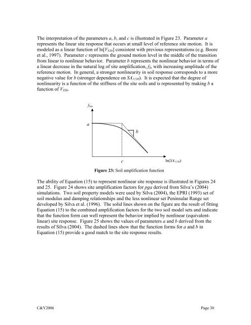
The interpretation of the parameters a, b, and c is illustrated in Figure 23. Parameter a
represents the linear site response that occurs at small level of reference site motion. It is
modeled as a linear function of ln[VS30] consistent with previous representations (e.g. Boore
et al., 1997). Parameter c represents the ground motion level in the middle of the transition
from linear to nonlinear behavior. Parameter b represents the nonlinear behavior in terms of
a linear decrease in the natural log of site amplification, fS, with increasing amplitude of the
reference motion. In general, a stronger nonlinearity in soil response corresponds to a more
negative value for b (stronger dependence on SA1130). It is expected that the degree of
nonlinearity is a function of the stiffness of the site soils and is represented by making b a
function of VS30.
fSite
a
c
Figure 23: Soil amplification function
ln(SA1130)
The ability of Equation (15) to represent nonlinear site response is illustrated in Figures 24
and 25. Figure 24 shows site amplification factors for pga derived from Silva’s (2004)
simulations. Two soil property models were used by Silva (2004), the EPRI (1993) set of
soil modulus and damping relationships and the less nonlinear set Peninsular Range set
developed by Silva et al. (1996). The solid lines shown on the figure are the result of fitting
Equation (15) to the combined amplification factors for the two soil model sets and indicate
that the function form can well represent the behavior implied by nonlinear (equivalentlinear)
site response. Figure 25 shows the values of parameters a and b derived from the
results of Silva (2004). The dashed lines show that the function forms for a and b in
Equation (15) provide a good match to the site response results.
C&Y2006 Page 30
b