Chiou and Youngs PEER-NGA Empirical Ground Motion Model for ...
Chiou and Youngs PEER-NGA Empirical Ground Motion Model for ... Chiou and Youngs PEER-NGA Empirical Ground Motion Model for ...
thrust earthquakes. The effect was attributed to the inability of the RRUP distance measure to capture the general proximity of a hanging wall site to rupture on the fault plane dipping beneath it. Chiou et al. (2000) performed extensive analyses of empirical and numerical modeling data for dipping fault ruptures and reached the same conclusion. They were able to remove the effect by using a root-mean-squared distance measure, RRMS. The hanging wall effect is seen in the PEER-NGA data. Figure 14 shows intra-event residuals for data from dip-slip earthquakes (both reverse/thrust and normal) plotted versus horizontal distance from a point above the top of the fault rupture. The dashed line is a locally-weighted least-squares fit to the residual. It shows an upward warp in the region where the hanging wall effect is expected to be present. The effect is also seen in the 1-D rock ground motion simulations conducted for the PEER-NGA project (Somerville et al., 2006). Figure 14: Intra-event residual for sites in the hanging wall (positive fault tip distance) and footwall (negative fault tip distance) from dip-slip earthquakes. Black dashed line is a locally-weighted leastsquares (lowess) fit to the residuals. Abrahamson and Silva (1997) included the hanging wall effect in their empirical ground motion model as a distance-dependent term with an abrupt switch from no effect to full effect as one crosses into the hanging wall region, defined as sites with a source-site angle, θSITE, between 60º and 120º. Boore et al. (1997) conclude that their use of RJB implicitly accounts for the hanging wall effect in that all site directly above the rupture have RJB = 0. Campbell and Bozorgnia (2003) introduces a smooth variation in the hanging wall effect by tapering the effect from a maximum at RJB = 0 to zero for RJB > 5 km while using RSEIS as the primary distance measure for assessing ground motion amplitudes. We have extended the concept proposed by Campbell and Bozorgnia (2003) by defining the hanging wall effect to be proportional to the factor [ 1− RJB / RRUP ] . Figures 15 through 17 illustrate the behavior of this function. Figure 15 shows a map view of a fault rupture with C&Y2006 Page 23
the top of rupture located at x = 0 and the fault dipping downward towards positive x. Figure 16 show the variation of the factor [ 1− RJB / RRUP] with location along three lines for the case when the top of rupture at x=0 is at the ground surface. Line 1 runs from negative values in the foot wall to positive values in the hanging wall. In the foot wall, RJB = RRUP and the hanging wall effect is zero. Thus the function acts as a switch equivalent to other formulations that only apply the effect on the hanging wall side of the fault. Lines 2 and 3 show the variation of [ 1− RJB / RRUP ] as one moves away from the rupture along strike. Line 2 is located near the top of the rupture and line 3 near the bottom. The function [ 1− RJB / RRUP ] decays much more rapidly for Line 2 than for Line 3. Most of Line 2 lies outside of the area typically defined as subject to the hanging wall effect while much of Line 3 for small values of y lines within the hanging wall area. The term [ 1− RJB / RRUP ] provides for a smooth transition in the level of the hanging wall effect throughout the along strike region. y 40 30 20 10 0 -10 -20 -30 -40 -30 -20 -10 0 10 20 30 40 50 60 70 80 90 100 1-Rjb/Rcld 1.2 1 0.8 0.6 0.4 0.2 x Figure 15: Map view of example fault rupture. 0 -40 -20 0 20 40 60 80 100 120 x (line 1) or y (lines 2 and 3) Line 1 (y=0) Line 2 (x=3) Line 3 (x=10) Rupture Figure 16: Variation of the term [ 1− RJB / RRUP ] with location for the three lines shown on Figure 15. Top of rupture is at the ground surface at x=0. Figure 17 shows the variation of the term [ 1− RJB / RRUP ] for the case when the top of rupture is located at a depth of 5 km. Now, the hanging wall effect extends into the footwall side of C&Y2006 Page 24 Line 1 Line 2 Line 3
- Page 1 and 2: Chiou and Youngs PEER-NGA Empirical
- Page 3 and 4: data are consistent with strong mot
- Page 5 and 6: Figure 1: Magnitude-distance-region
- Page 7 and 8: Figure 2: Empirical ground motion d
- Page 9 and 10: EQID Earthquake M Table 3: Inferred
- Page 11 and 12: Site Average Shear Wave Velocity: A
- Page 13 and 14: Figure 6: Relationship between VS30
- Page 15 and 16: 1 ) ∝ C2 × M + ( C2 − C ) × l
- Page 17 and 18: Figure 9: Peak acceleration data fr
- Page 19 and 20: C4+C5M slowly and the value of the
- Page 21 and 22: allows the interpretation of the co
- Page 23: Figure 13: Coefficients resulting f
- Page 27 and 28: Figure 18: Intra-event residuals fo
- Page 29 and 30: Figure 21: Variation of HW* with ma
- Page 31 and 32: The interpretation of the parameter
- Page 33 and 34: to the PEER-NGA pga data selected f
- Page 35 and 36: EFFECT OF DATA TRUNCATION The initi
- Page 37 and 38: term [ 1 Φ( y ( θ ) + τ ⋅ z ,
- Page 39 and 40: Table 4: Estimate of Anelastic Atte
- Page 41 and 42: data truncated at a maximum distanc
- Page 43 and 44: faulting earthquakes at long period
- Page 45 and 46: Slope -1.5 -1.0 -0.5 0.0 0.5 1.0 0.
- Page 47 and 48: C&Y2006 Page 46 Table 5: Coefficien
- Page 49 and 50: c1 of T0.010S c1 of T1.000S MODEL R
- Page 51 and 52: esid 1 0 -1 -2 resid resid 1 0 -1 -
- Page 53 and 54: esid resid resid 1 0 -1 -2 1 0 -1 -
- Page 55 and 56: esid 2 1 0 -1 -2 SCEC Version 2 0 2
- Page 57 and 58: Amplification w.r.t. Vs30 = 1130 m/
- Page 59 and 60: Sa(g) Sa(g) 10 1 0.1 0.01 10 1 0.1
- Page 61 and 62: Sa (g) Sa (g) 1 0.1 0.01 0.001 0.00
- Page 63 and 64: Sa (g) Sa (g) 1 0.1 0.01 0.001 1 0.
- Page 65 and 66: EXAMPLE CALCULATIONS FORTRAN routin
- Page 67 and 68: Table 6: Example Calculations Perio
- Page 69 and 70: REFERENCES Abrahamson, N.A., and Si
- Page 71 and 72: Frankel, A., A. McGarr, J. Bicknell
- Page 73 and 74: Appendix A Recordings from PEER-NGA
thrust earthquakes. The effect was attributed to the inability of the RRUP distance measure to<br />
capture the general proximity of a hanging wall site to rupture on the fault plane dipping<br />
beneath it. <strong>Chiou</strong> et al. (2000) per<strong>for</strong>med extensive analyses of empirical <strong>and</strong> numerical<br />
modeling data <strong>for</strong> dipping fault ruptures <strong>and</strong> reached the same conclusion. They were able to<br />
remove the effect by using a root-mean-squared distance measure, RRMS.<br />
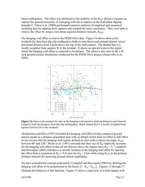
The hanging wall effect is seen in the <strong>PEER</strong>-<strong>NGA</strong> data. Figure 14 shows intra-event<br />
residuals <strong>for</strong> data from dip-slip earthquakes (both reverse/thrust <strong>and</strong> normal) plotted versus<br />
horizontal distance from a point above the top of the fault rupture. The dashed line is a<br />
locally-weighted least-squares fit to the residual. It shows an upward warp in the region<br />
where the hanging wall effect is expected to be present. The effect is also seen in the 1-D<br />
rock ground motion simulations conducted <strong>for</strong> the <strong>PEER</strong>-<strong>NGA</strong> project (Somerville et al.,<br />
2006).<br />
Figure 14: Intra-event residual <strong>for</strong> sites in the hanging wall (positive fault tip distance) <strong>and</strong> footwall<br />
(negative fault tip distance) from dip-slip earthquakes. Black dashed line is a locally-weighted leastsquares<br />
(lowess) fit to the residuals.<br />
Abrahamson <strong>and</strong> Silva (1997) included the hanging wall effect in their empirical ground<br />
motion model as a distance-dependent term with an abrupt switch from no effect to full effect<br />
as one crosses into the hanging wall region, defined as sites with a source-site angle, θSITE,<br />
between 60º <strong>and</strong> 120º. Boore et al. (1997) conclude that their use of RJB implicitly accounts<br />
<strong>for</strong> the hanging wall effect in that all site directly above the rupture have RJB = 0. Campbell<br />
<strong>and</strong> Bozorgnia (2003) introduces a smooth variation in the hanging wall effect by tapering<br />
the effect from a maximum at RJB = 0 to zero <strong>for</strong> RJB > 5 km while using RSEIS as the primary<br />
distance measure <strong>for</strong> assessing ground motion amplitudes.<br />
We have extended the concept proposed by Campbell <strong>and</strong> Bozorgnia (2003) by defining the<br />
hanging wall effect to be proportional to the factor [ 1−<br />
RJB<br />
/ RRUP<br />
] . Figures 15 through 17<br />
illustrate the behavior of this function. Figure 15 shows a map view of a fault rupture with<br />
C&Y2006 Page 23


