PDF Full Text - DSP-Book

Derivation of Estimator Equations 541 

In both cases (3 18) assumes E[x(T~)] = 0. The modification for other 

initial conditions is straightforward (see Problem 6.3.20). Differentiating 

(3 18), we have 

dj2(t) 

- = h,(t, t) r(t) + 

t as4 

- 

4 

r(7) dT. 

dt s at 

(319 

Tf 

Substituting (3 17) into the second term on the right-hand side of (3 19) and 

using (3 18), we obtain 

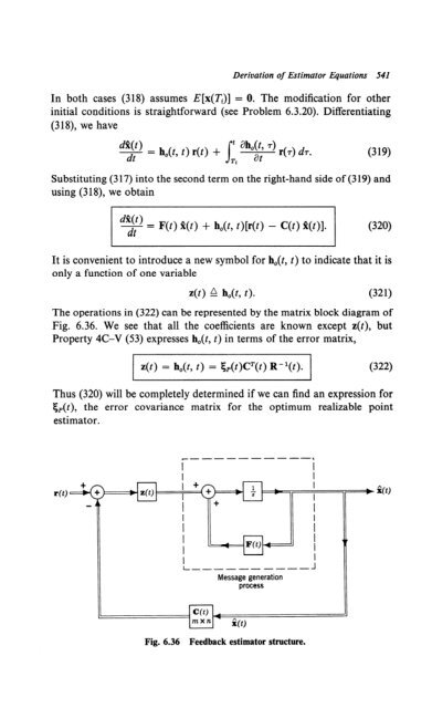
‘F = F(t) 2(t) + h,(t, t)[r(t) - C(t) R(t)]. (320) 

It is convenient to introduce a new symbol for h,(t, t) to indicate that it is 

only a function of one variable 

z(t) Li h,(t, t). (321) 

The operations in (322) can be represented by the matrix block diagram of 

Fig. 6.36. We see that all the coefficients are known except z(t), but 

Property 4C-V (53) expresses h,(t, t) in terms of the error matrix, 

, 

z(t) = h,(t, t) = &(t)CT(t) R-‘(t). (322) 

Thus (320) will be completely determined if we can find an expression for 

gp(t), the error covariance matrix for the optimum realizable point 

estimator. 

-- 

--me 

I I 

I 

I 

+ 

--me-, 

1 

I 

+s- 

‘ I 

I I 

I I 

I 

l 

4 

I 

I 

L- --- 

: WI 

--e 

4 h 

--em 

I 

I 

J 

Message generation 

process 

Fig. 6.36 Feedback estimator structure. 

I 

I 

I 

___r w

542 6.3 Kalman-Bucy Filters 

Step 3. We first find a differential equation for the error x,(t), where 

Differentiating, we have 

xc(t) a, x(t) - 2(t). (323) 

d&(0 dW 

-=-- 

d2(t) P. 

dt dt dt 

Substituting (302) for the first term on the right-hand side of (324), sub- 

stituting (320) for the second term, and using (309, we obtain the desired 

equation 

y = [F(t) - z(t) C(olXm - z(t) w(t) + G(t) u(t). 

The last step is to derive a differential equation for gp(t). 

Step 4. Differentiating 

we have 

w> A m&) X,Tw 

I 

&(0 - 

dt 

= x&) 

dJbT(t) 

--&- 

Substituting (325) into the first term of (327), we have 

1 

= E{[F(t) - z(t) WI w xt-‘w 

- z(t) w(t) q’(t) + G(t) u(t) xET(t)}- 

l 

(329 

(326) 

(327) 

(328) 

Looking at (325), we see xc(t) is the state vector for a system driven by 

the weighted sum of two independent white noises w(t) and u(t). Therefore 

the expectations in the second and third terms are precisely the same type 

as we evaluated in Property 13 (second line of 266). 

E dxdt) 

[ -Jj--- xc’(t) I = F(t) b(t) - z(t) c(t> w> 

+ $z(t) R(t) z’(t) + + G(t)Q GT(t). (329 

Adding the transpose and replacing z(t) with the right-hand side of (322), 

we have 

y’= F(t) gp(t) + gp(t) FT(t) - &(t) CT(t) R-l(t) C(t) Ep(t) 

+ G(t)Q GT(t), (330) 

which is called the variance equation. This equation and the initial condition 

w-i) = EMT,) x,Tml (331) 

determine &Jt) uniquely. Using (322) we obtain z(t), the gain in the 

optimal filter.


Observe that the variance equation does not contain the received signal. 

Therefore it may be solved before any data is received and used to deter- 

mine the gains in the optimum filter. The variance equation is a matrix 

equation equivalent to yt2 scalar differential equations. However, because 

gp(t) is a symmetric matrix, we have &+z(n + 1) scalar nonlinear coupled 

differential equations to solve. In the general case it is impossible to obtain 

an explicit analytic solution, but this is unimportant because the equation 

is in a form which may be integrated using either an analog or digital 

computer. 

The variance equation is a matrix Riccati equation whose properties 

have been studied extensively in other contexts (e.g., McLachlan [3i]; 

Levin [32]; Reid [33], [34]; or Coles [35]). To study its behavior adequately 

requires more background than we have developed. Two properties are of 

interest. The first deals with the infinite memory, stationary process case 

(the Wiener problem) and the second deals with analytic solutions. 

Property 15. Assume that Tf is fixed and that the matrices F, G, C, R, and 

Q are constant. Under certain conditions, as t increases there will be an 

initial transient period after which the filter gains will approach constant 

values. Looking at (322) and (330), we see that as fp(t) approaches zero 

the error covariance matrix and gain matrix will approach constants. We 

refer to the problem when the condition ep(t) = 0 is true as the steady- 

state estimation problem. 

The left-hand side of (330) is then zero and the variance equation 

becomes a set of +z(rt + 1) quadratic algebraic equations. The non- 

negative definite solution is gP. 

Some comments regarding this statement are necessary. 

1. How do we tell if the steady-state problem is meaningful? To give 

the best general answer requires notions that we have not developed [23]. 

A suficient condition is that the message correspond to a stationary 

random process. 

2. For small y2 it is feasible to calculate the various solutions and select 

the correct one. For even moderate yt (e.g. yt = 2) it is more practical to 

solve (330) numerically. We may start with some arbitrary nonnegative 

definite gP(7Yi) and let the solution converge to the steady-state result (once 

again see 1231, Theorem 4, p. 8, for a precise statement). 

3. Once again we observe that we can generate &(t) before the data is 

received or in real time. As a simple example of generating the variance 

using an analog computer, consider the equation: 

wt> - = -2k &(t) - 

dt 

$- tp2(t) + 2kP. 

0 

(332)

544 6.3 Kalman-Bucy FiZtet-s 

(This will appear in Example 1.) A simple analog method of generation is 

shown in Fig. 6.37. The initial condition is &(&) = P (see discussion in 

the next paragraph). 

4. To solve (or mechanize) the variance equation we must specify 

&( T$). There are several possibilities. 

(a) The process may begin at ZYj with a known value (i.e., zero 

variance) or with a random value having a known variance. 

(b) The process may have started at some time to which is much 

earlier than T. and reached a statistical steady state. In Property 

14 on p. 533 we derived a differential equation that R,(c) satisfied. 

If it has reached a statistical steady state, A,(t) = 0 and (273) 

reduces to 

0 = FA, + A,FT + GQGT. (333a) 

This is an algebraic equation whose solution is A,. Then 

b(T) = Ax (3333) 

if the process has reached steady state before Tie In order for the 

unobserved process to reach statistical steady state (k,(t) = 0), 

it is necessary and sufficient that the eigenvalues of F have 

negative real parts. This condition guarantees that the solution 

to (333) is nonnegative definite. 

In many cases the basic characterization of an unobserved 

stationary process is in terms of its spectrum S&). The elements 

1 J 

r -I 

2 

).- 4 

\ 

NO 

- 

1 Squarer -z 

Fig. 6.37 Analog solution to variance equation.


in A, follow easily from S&O). As an example consider the state 

vector in (191), 

xi = 

If y(t) is stationary, then 

or, more generally, 

A x,fk = 

Note that, for 

dcf - l’y(t) 

,&W-l ’ i= 1,2 ,..., n. (334a) 

A x,11 = 

s c0 

--a0 

s 

Go 

-00 

this particular state vector, 

(3343) 

A x,ik = 0 when i + k is odd, (334d) 

because S’&) is an even function. 

A second property of the variance equation enables us to obtain analytic 

solutions in some cases (principally, the constant matrix, finite-time 

problem). We do not use the details in the text but some of the problems 

exploit them. 

Property 16. The variance equation can be related to two simultaneous 

linear equations, 

or, equivalently, 

y = F(t) VI(t) + G(t) QCF(t) vz(t), 

dv,w 

- = CT(t) R-l(t) C(t) v&) - F(t) vz(t), 

dt 

F(t) I G(t) 

1 [ QGT(O = .------------------ I I-------------. vi(t) 

I[ I . (336) 

CT(t) R-l(t) C(t) : - FT(t) v&l 

Denote the transition matrix of (336) by 

T(4 T,) = 

Then we can show 1321, 

Tll(4 T,) 1 Tl&, n 

1 

-------------------- I ’ 

T& G) i Tm(4 n 

(339 

(337) 

b(t> = ITll(4 T) km + T12(t, n1 CT& n km + Tdt, TN- l* (338)


When the matrices of concern are constant, we can always find the transi- 

tion matrix T (see Problem 6.3.21 for an example in which we find T by 

using Laplace transform techniques. As discussed in that problem, we 

must take the contour to the right of all the poles in order to include all 

the eigenvalues) of the coefficient matrix in (336). 

In this section we have transformed the optimum linear filtering problem 

into a state variable formulation. All the quantities of interest are expressed 

as outputs of dynamic systems. The three equations that describe these 

dynamic systems are our principal results. 

The Estimator Equation. 

The Gain Equation. 

The Variance Equation. 

‘9 = F(t) 9(t) + z(t)[r(t) - C(t) 2(t)]. 

z(t) = &a(t) CT(t) R--l(t). 

c 

1 WV 

y = F(t) EP(~) + b(t) FT(t) - b(t) CT(t) R- ‘(t> C(t) b(t) 

+ G(t) QGT(t). (341) 

To illustrate their application we consider some simple examples, chosen 

for one of three purposes: 

1. To show an alternate approach to a problem that could be solved 

by conventional Wiener theory. 

2. To illustrate a problem that could not be solved by conventional 

Wiener theory. 

3. To develop a specific result that will be useful in the sequel. 

6.3.3 Applications 

In this section we consider some examples to illustrate the application 

of the results derived in Section 6.3.2. 

Example 1. Consider the first-order message spectrum 

2kP 

slso) = -. 

o2 + k2 

(342)

Applications 547 

In this case x(t) is a scalar; x(t) = a(t). If we assume that the message is not modulated 

and the measurement noise is white, then 

The necessary quantities follow by inspection : 

r(t) = x(t) + w(t). (343) 

F(t) = -k, 

G(t) = 1, 

C(t) = 1, 

Q = 2kP, 

R(t) = $ 

Substituting these quantities into (339), we obtain the differential equation for the 

optimum estimate : 

d$(t) 

- = -kZ(t) + z(t)[r(t) - a(t)]. 

dt 

(3W 

(345) 

The resulting filter is shown in Fig. 6.38. The value of the gain z(t) is determined by 

solving the variance equation. 

First, we assume that the estimator has reached steady state. Then the steady-state 

solution to the variance equation can be obtained easily. Setting the left-hand side 

of (341) equal to zero, we obtain 

0 = -2kfm - f;a, + + 2kP. (346) 

0 

where fPa, denotes the steady-state variance. 

There are two solutions to (346); one is positive and one is negative. Because tpoo is 

a mean-square error it must be positive. Therefore 

(recall that A = 4P/kN,). From (340) 

f Pm = k?(-1 + driin) (34-a 

z(m) Li za, = 5‘pooR-1 = k(-1 + 41 + A). (348) 

Fig. 6.38 Optimum filter: example 1.


Clearly, the filter must be equivalent to the one obtained in the example in Section 

6.2. The closed loop transfer function is 

Substituting (348) in (349), we have 

Ho(jw) = ‘* 

jw + k + zo3* 

HOW = 

k(dl+ - 1) 

jo + kdl+’ 

(349) 

which is the same as (94). 

The transient problem can be solved analytically or numerically. The details of 

the analytic solution are carried out in Problem 6.3.21 by using Property 16 on p. 545. 

The transition matrix is 

T(Ti + 7, Ti) = I 

k 

cash (~7) - 7 sinh (YT) i 

2kP 

7 sinh (~7) 

--------------------I 1 

I 

I 

--------------------. 

’ 

2 

G sinh (~7) i cash (~7) + 

(351) 

k 

; sinh (~7) 

0 

I 

where 

y 4i kd+h. (352) 

If we assume that the unobserved message is in a statistical steady state then 2 (Ti) = 0 

and tp(Ti) = P. [(342) implies a(t) is zero-mean.] Using these assumptions and (351) 

in (338), we obtain 

As t-+-co, wehave 

2kP No 

lim fp(t + Tr) = y+k = 7 [y - k] = fp*, 

t+a 

(354) 

which agrees with (347). In Fig. 6.39 we show the behavior of the normalized error 

as a function of time for various values of A. The number on the right end of each 

curve is &( 1.2) - &. This is a measure of how close the error is to its steady-state value. 

Example 2. A logical generalization of the one-pole case is the Butterworth family 

defined in (153) : 

S&w: n) = - 

2nP sin (n/2n) 

k (1 + (u/k)2n)’ 

(355) 

To formulate this equation in state-variable terms we need the differential equation of 

the message generation process. 

@j(t) + J3n - 1 atn- l’(t) + l 

l l +po 

a(t) = u(t)= (356) 

The coefficients are tabulated for various n in circuit theory texts (e.g., Guillemin 

[37] or Weinberg [38]). The values for k = 1 are shown in Fig. 6.40a. The pole 

locations for various n are shown in Fig. 6.406. If we are interested only in the

fp w 

n 

0.8 

0.7 

0.6 

0.5 

- R=& 

- 

- 

R=:l 

F=-1 

G=l 

0.001 

Q=2 

C=l 

tpKu = 1 

I I I I I I I I I I I I 1 

0 0.1 0.2 0.3 0.4 0.5 0.6 0.7 0.8 0.9 1.0 1.1 1.2 

t----t 

Pn-1 

Fig. 6.39 Mean-square error, one-pole spectrum. 

1.414 1 .ooo 

2.000 2.000 

2.613 3.414 

3.236 5.236 

3.864 7.464 

4.494 10.103 

Pn-2 Pn-3 Pn-4 

-T- 

1 .ooo 

2.613 1.000 

5.236 3.236 

9.141 7.464 

14.606 14.606 

Pn-5 

1.000 

3.864 

10.103 

Q(n)(t) + pn - 1 dn - l)(t) + l l . + p0 a(0 = 40 

h-6 Pn-7 

1 .ooo 

4.494 1 .ooo 

Fig. 6.40 (a) Coefficients in the differential equation describing the Butterworth 

spectra [ 381. 

549

5.50 6.3 Kalman-Bucy Filters 

n=l 

n=3 

7F 

/ 

! 

\ 

\ 

\ 

* 

‘- 

n=2 

n=4 

Poles are at s=exp(jn(2m+n-l)):m= 1,2,..., 2n 

Fig. 6.40 (6) pole plots, Butterworth spectra. 

message process, we can choose any convenient state representation. An example is 

defined by (191), 

XL0 = a(t) 

x2(t) = b(t) = A,(t) 

x3(t) = 6(t) = 2,(t) 

. 

wn 

xn(t) = a(“- *j(t) = &-l(t) 

*a(t) = - 2 pk - 1 atkB1)(t) + u(t) 

k=l 

=- 2 pk-1 Xk(f) + dt) 

k=l

l l l 

Applications 55 I 

e. 

The resulting F matrix for any n is given by using (356) and (193). The other 

quantities needed are 

[I 

0 

G(t) = ; 

wo 

; 

C(t) = [l I 0 : ; O] (359) 

R(t) = ?- (361) 

kll0 

From (340) we observe that z(t) is an n x 1 matrix, 

z(t) 2 

L 

&2(t) 

I 

= N 

9 

0 : 

(362) 

Il:(t 1 

&(t) = 2,(t) + + S‘ll(t)[~o) - &WI 

0 

$20) = 2,(t) + + 512MW - &(Ol 

0 

: 

. 

3*(t) = -poZl(t) - pl&(t)- ’ ’ ’ -Pn - 1 h(t) + ~~ 

2 41n(t)[r(t 1 - M)l* 

The block diagram is shown in Fig. 6.41. 

Fig. 6.41 Optimum filter: &h-order Butterworth message. 

(363)

552 6.3 Kulman-Bucy Filters 

0.8 

0.6 

MO 0.5 

0.4 

0.3 

0.2 

0.1 

0 

0.3 

;j,G=Ll,C=[l O] Q=2I/z- 

--L, 

I I I I I I I I I I 

0.1 0.2 0.3 0.4 0.5 0.6 0.7 0.8 0.9 1.0 1.1 1.2 

t----t 

I I I I I I I I I I I I - 

0.1 0.2 0.3 0.4 0.5 0.6 0.7 0.8 0.9 1.0 1.1 1.2 

t---s 

Fig. 6.42 (a) Mean-square error, second-order Butterworth; (6) filter gains, second- 

order Butterworth. 

To find the values of &(t), . . . , II,(t), we solve the variance equation. This could 

be done analytically by using Property 16 on p. 545, but a numerical solution is much 

more practical. We assume that Tt = 0 and that the unobserved process is in a 

statistical steady state. We use (334) to find &(O). Note that our choice of state 

variables causes (334d) to be satisfied. This is reflected by the zeros in &(O) as shown 

in the figures. In Fig. 6.42~~ we show the error as a function of time for the two-pole 

case. Once again the number on the right end of each curve is &( 1.2) - tpa,. We see 

that for t = 1 the error has essentially reached its steady-state value. In Fig. 6.426 

we show the term &(t). Similar results are shown for the three-pole and four-pole 

cases in Figs. 6.43 and 6.44, respective1y.t In all cases steady state is essentially 

reached by t = 1. (Observe that k = 1 so our time scale is normalized.) This means 

t The numerical results in Figs. 6.39 and 6.41 through 6.44 are due to Baggeroer [36].

-0.6’ 

-0.1 - 

0.012- 

Q=3 

, , , , , ,- 

0.3 0.4 0.5 0.6 0.7 0.8 0.9 1.0 1.1 1.2 

t----t 

0.1 0.2 0.3 0.4 0.5 0.6 0.7 0.8 0.9 1.0 1.1 1.2 

t- 

I I I I I I I I I I I I - 

(Note negative scale) 

O* I I I I I I I I I I I 

0.1 0.2 0.3 0.4 0.5 0.6 0.7 0.8 0.9 1.0 1.1 1.2 

Fig. 6.43 (a) Mean-square error, third-order Butterworth; (21) filter gain, third-order 

Butterworth; (c) filter gain, third-order Butterworth. 

R=j/,, 

553

E12W 

0.8 

o*f\ 

0.4 

0.3 I 

-2.61 -3.41 

d 

I [I 

’ 0’ ’ 

0 G=O Q = 3.06 

1 0 

-2.61 1 

’ 

c = [l 0 0 01 

\ \l - 

0.2 - 0 

1 

0.1 4Pvo = ,[, -0.i4 

0 -0.414 0 

0.414 0 -0.414 

0 0.414 0 

0 -0.414 0 1 

0, , , , 

0 0.1 0.2 0.3 0.4 0.5 0.6 0.7 0.8 0.9 1.0 1.1 

0.25 

0.2 

0.1 

-0.1 

0 

t 

0.1 0.2 0.3 0.4 0.5 0.6 0.7 0.8 0.9 1.0 1 .l 1.2 

I I I I I I I I I I 

I 

0.1 

I 

0.2 

I 

0.3 

I 

0.4 

I 

0.5 

I 

0.6 

I 

0.7 

I 

0.8 0.9 1.0 

I 

1.1 

i 

I 

1.2 

Fig. 6.44 (a) Mean-square error, fourth-order Butterworth; (b) filter gains, fourth- 

order Butterworth; (c) filter gains, fourth-order Butterworth. 

!

fl4W 

do - (Note negative scale) 

Fig. 6.44 (d) filter gains, fourth-order Butterworth. 


that after t = 1 the filters are essentially time-invariant. (This does not imply that all 

terms in &(t) have reached steady state.) A related question, which we leave as an 

exercise, is, “If we use a time-invariant filter designed for the steady-state gains, how 

will its performance during the initial transient compare with the optimum time- 

varying filter ?” (See Problems 6.323 and 6.326.) 

Example 3. The two preceding examples dealt with stationary processes. A simple 

nonstationary process is the Wiener process. It can be represented in differential 

equation form as 

Observe that even though the coefficients in the differential equation are constant 

the process is nonstationary If we assume that 

the estimator follows easily 

where 

and 

R(t) = G u(t), 

x(0) = 0. 

r(t) = x(t) + w(t), (365) 

i(t) = dew - WI, (366) 

dt) = f IPW (367) 

0 

I() pt = -$ gp2(t) + G'Q. (368) 

0 

The transient problem can be solved easily by using Property 16 on p. 545 (see 

Problem 6.3.25). The result is 

&(t) = (2 G”Q)’ = 9 (369 

where y = [2G2Q/No]K [Observe that (369) is not a limiting case of (353) because the 

initial condition is different.] As t --+ 00, the error approaches steady state. 

Ipa, = (+ G~Q)' (370) 

[(370) can also be obtained directly from (368) by letting I=(t) = 0.1 

wo


Fig. 6.45 Steady-state filter: Example 3. 

The steady-state filter is shown in Fig. 6.45. It is interesting to observe that this 

problem is not included in the Wiener-Hopf model in Section 6.2. A heuristic way to 

include it is to write 

S&J) = =I 

aJ2 + c2 

(371) 

solve the problem by using spectral factorization techniques, and then let c -3 0. 

It is easy to verify that this approach gives the system shown in Fig. 6.45. 

Example 4. In this 

problem : 

example we derive a canonic receiver model for the following 

l l l 

1. The message has a rational spectrum in which the order of the numerator as a 

function of w2 is at least one smaller than the order of the denominator. We use the 

state variable model described in Fig. 6.30. The F and G matrices are given by (212) 

and (213), respectively (Canonic Realization No. 2). 

2. The received signal is scalar function. 

3. The modulation matrix has unity in its first column and zero elsewhere. In 

other words, only the unmodulated message would be observed in the absence of 

measurement noise, 

C(t) = [l : 0 01. (372) 

The equation describing the estimator is obtained from (339), 

and 

3(t) = F%(t) + z(t)[r(t) - RI(t)] (373) 

AS in Example 2, the gains are simply 2/N. times the first row of the error matrix. 

The resulting filter structure is shown in Fig. 6.46. As t -+ a, the gains become 

constant. 

For the constant-gain case, by comparing the system inside the block to the two 

diagrams in Fig. 6.30 and 31a, we obtain the equivalent filter structure shown in 

Fig. 6.47. 

Writing the loop filter in terms of its transfer function, we have 

2 

G,,(s) = - 

511sn - l + l l l + e1n 

No sn + Pn-lSnB1 + l . l + PO’ 

(375)

I 

I 

I 

B-----m- ------------s- 

r 

1 

s 


I 

I 

I 

A 

I 

I 

jj 

tt 

A A 

L B------m ---w-B ----- w-- J 

Loop filter 

Fig. 6.46 Canonic estimator: stationary messages, statistical steady-state. 

Thus the coefficients of the numerator of the loop-filter transfer function correspond 

to the first column in the error matrix. The poles (as we have seen before) are identical 

to those of the message spectrum. 

Observe that we still have to solve the variance equation to obtain the numerator 

coefficients. 

Example 5A [23]. As a simple example of the general case just discussed, consider 

the message process shown in Fig. 6.48a. If we want to use the canonic receiver 

structure we have just derived, we can redraw the message generator process as shown 

in Fig. 6.486. 

We see that 

p1 = k, pO=O, bl=O, bO=l. (376) 

Fig. 6.47 Canonic estimator : stationary messages, statisticat steady-state. 

\I 

1 

I 

I 

I 

I 

I 

I 

I 

I 

I 

I 

I 

-T- 

I 

I 

I 

I 

I 

I 

I 

I 

I


u(t) 

Fig. 6.48 Systems for example 5A : (a) message generator; (b) analog representation; 

(c) optimum estimator. 

Then, using (212) and (213), we have 

F= [ik ;], G=[;], c=[l 01 

Q = q, R = NO/2. 

The resulting filter is just a special case of Fig. 6.47 as shown in Fig. 6.48.

The variance equation in the steady state is 

Thus the steady-state errors are 

I 12 

-Mu + 522 -- 2 

No 

=s 2qvr 

2x ( ) 

6 11 I‘ 12 = 0, 

2 

j(g La2 = q* 

gll = $‘{-k + [k2 + 2($!-)‘]‘}e 


(378) 

(379) 

We have taken the positive definite solution. The loop filter for the steady-state case 

G (s) 

lo = 

{-k + [k2 + 2($-)K]K}s + ($)’ 

s(s + k) 

. 

(380) 

Example SB. An interesting example related to the preceding one is shown in Fig. 

6.49. We now add A and B subscripts to denote quantities in Examples 5A and SB, 

respectively. We see that, except for some constants, the output is the same as in 

Example 5A. The intermediate variable x2,(t), however, did not appear in that 

realization. 

We assume that the message of interest is xz,(t). In Chapter II.2 we shall see the 

model in Fig. 6.49 and the resulting estimator play an important role in the FM 

problem. This is just a particular example of the general problem in which the 

message is subjected to a linear operation befire transmission. There are two easy 

ways to solve this problem. One way is to observe that because we have already 

solved Example SA we can use that result to obtain the answer. To use it we must 

express x2,(t) as a linear transformation of xl,(t) and x2,(t), the state variables in 

Example SA. 

p xz,(t) = &,(t) (381) 

and 

x1,(0 = x1,0, (382) 

if we require 

Observing that 

we obtain 

qA = r6’qB* (383) 

x2,4(t 1 = k xl,(t) + h,(t), (384) 

fl x+3(t) = 21,(t) = -kXl,(t) + x2,(t). (385) 

l XlBW 

1 

s+K X2J3(t) 

Fig. 6.49 Message generation, example SB. 

%


Now minimum mean-square error filtering commutes over linear transformations. 

(The proof is identical to the proof of 2.237.) Therefore 

Rz,(t) = 2 [k &,(t) + $,(t>l. (386) 

Observe that this is not equivalent to letting /32,,(t) equal the derivative of Z,,(t). Thus 

1 

22,(t) # p %*(t). (3W 

With these observations we may draw the optimum filter by modifying Fig. 6.48. 

The result is shown in Fig. 6.50. The error variance follows easily: 

Alternatively, if we had not solved Example SA, we would approach the problem 

directly. We identify the message as one of the state variables. The appropriate 

matrices are 

and 

F= [I -“,I, G=[;], C=[l 01 (389) 

Q = qB* MO 

Fig. 6.50 Estimator for example 5B.


The structure of the estimator is shown in Fig. 6.51. The variance equation is 

Al(t) = 2Pf12(0 - jg f 31 (0 9 

0 

412(t) = Bfm(t) - kf12W - j$ fllU)fdO, 

0 

#22(t) = - 2kf 22(t) - j$ f&(t) + !b 

0 

(39~) 

Even in the steady state, these equations appear difficult to solve analytically. In 

this particular case we are helped by having just solved Example 5A. Clearly, fll(t) 

must be the same in both cases, if we let qA = f12qB. From (379) 

f ll,co = !ip{-l + [l + gg!yS} 

The other gain 5 12,co now follows easily 

f 

k2Nou2 

12.00 = -* 4P 

(393) 

Because we have assumed that the message of interest is x2(t), we can also easily 

calculate its error variance: 

4 22.a~ 

1 

= - 2k 

It is straightforward to verify that (388) and (394) give the same result and that the 

block diagrams in Figs. 6.50 and 6.51 have identical responses between r(t) and a,(t). 

The internal difference in the two systems developed from the two different state 

representations we chose. 

Fig. 6.51 Optimum estimator: example 5B (form #2). 

wo


Example 6. Now consider the same message process as in Example 1 but assume that 

the noise consists of the sum of a white noise and an uncorrelated colored noise, 

and 

no = r&(t) + w(t) (395) 

sew 

2M’c 

=-. w2 + kc2 ww 

As already discussed, we simply include nc(t) as a component in the state vector. 

Thus, 

and 

The gain matrix z(t) becomes 

or 

x(t) a (397) 

1 0 

G(t) = [ 0 1) 1 

The equation specifying the estimator is 

d%(t) 

dt 

or in terms of the components 

(399) 

c(t) = 11 11, WV 

z(t) = $ glw CT(t), 

0 

(403) 

zu(t) = + [&1(t) + 512w1, (404) 

0 

zzrw = f [512(t) + t22w1. (405) 

0 

= F(t) ji(t) + z(t)[r(t) - C(t) g(t)], 

&(t) 

- = -k&(t) + zll(t)[r(t) - a,(t) - h(t)19 

dt 

d%(f) 

- = -k,a,(t) + zzl(t)[r(t) - &(t) - $2(t)]- 

dt 

(406) 

(407) 

(408) 

The structure is shown in Fig. 6.52a. This form of the structure exhibits the 

symmetry of the estimation process. Observe that the estimates are coupled through 

the feedback path.

0 a 


Fig. 6.52 Optimum estimator: colored and white noise (statistical steady-state). 

An equivalent asymmetrical structure which shows the effect of the colored noise 

on the message is shown in Fig. 6.526. To find the gains we must solve the variance 

equation. Substituting into (341), we find 

Ill@) = - Wdt) - 

2 

No (MO + MtD2 + 2W (409) 

k,,co = -(k + kc)Sdt) - x 2 (MO + g12(0)(&2(0 + g22(t)), (410) 

#22co = - 2kcQdt) - $ &z(t) + MO12 + 2kcPc. (410 

Two comments are in order. 

1. The system in Fig. 6.52a exhibits all of the essential features of the canonic 

structure for estimating a set of independent random processes whose sum is observed

564 6.3 Kalman-Buy Filters 

in the presence of white noise (see Problem 6.3.31 for a derivation of the general 

canonical structure). In the general case, the coupling arises in exactly the same 

manner. 

2. We are tempted to approach the case when there is no white noise (No = 0) 

with a limiting operation. The difficulty is that the variance equation degenerates. 

A derivation of the receiver structure for the pure colored noise case is discussed in 

Section 6.3.4. 

Example 7. The most common example of a multiple observation case in communications 

is a diversity system. A simplified version is given here. Assume that the 

message is transmitted over m channels with known gains as shown in Fig. 6.53. 

Each channel is corrupted by white noise. The modulation matrix is m x n, but only 

the first column is nonzero: 

C(t) = 

[ 

c2 ; 

1 

c2 ; 0 a [c f 01. 

. I 

Cm ! 

(412) 

For simplicity we assume first that the channel noises are uncorrelated. Therefore 

R(t) is diagonal : 

R(t) = 

‘N 

2 0 

N2 

2 

0 Xl 

. 2. 

Fig. 6.53 Diversity system. 

(413)

The gain matrix z(t) is an n x m matrix whose ijth element is 


The general receiver structure is shown in Fig. 6.54a. We denote the input to the 

inner loop as v(t), 

v(t) = z(NW - C(t) WI. (41 Sa) 

Using (412)-(414), we have 

Vi(t) = &l,[ j: 2 r,(t) - (2 ~)"'(')]. 

jY1 j j=l 

(415b) 

We see that the first term in the bracket represents a no-memory combiner of the 

received waveforms. 

Denote the output of this combiner by rc(t), 

m 2cj 

t-c(t) = )‘ - uJ(t). 

j&i w 

(416) 

We see that it is precisely the maximal-ratio-combiner that we have already en- 

countered in Chapter 4. The optimum filter may be redrawn as shown in Fig. 6.546. 

We see that the problem is reduced to a single channel problem with the received 

waveform rc(t), 

rcw = ( 2 1 

m z a(t) + 3 2 nj(t). 

j=l j=l 

r(t) 

I 3 Loop filter w > 

, m 

Fig. 6.54 Diversity receiver. 

(417a)


The modulation matrix is a scalar 

and the noise is 

c = 

n&) 

* 2c, 

a C - njW. 

j=l w 

If the message a(t) has unity variance then we have an effective power of 

and an effective noise level of 

Ned - * zc 2 

2 - j=l c Nj j ’ 

(417b) 

(417c) 

(419) 

Therefore all of the results for the single channel can be used with a simple scale 

change; for example, for the one-pole message spectrum in Example 1 we would have 

where 

f (-1 + 1/G-z+, (420) 

Similar results hold when R(t) is not diagonal and when the message is nonstationary. 

(421) 

These seven examples illustrate the problems encountered most fre- 

quently in the communications area. Other examples are included in the 

problems. 

6.3.4 Generalizations 

Several generalizations are necessary in order to i .nclude other problems 

of interest. We discuss them briefly in this section. 

Prediction. In this case d(t) = x(t + a>, where a is positive. We can 

show easily that 

S(t) = +(t + a, t) 2(t), a > 0, (422) 

where +(t, 7) is the transition matrix of the system, 

k(t) = F(t) x(t) + G(t) u(t) (423) 

(see Problem 6.3.37). 

When we deal with a constant parameter system, 

and (422)& becomes 

+(t + a, t) = eFa, 

&t> = eFa 2(t).

Generalizations 567 

Firtering with Delay. In this case d(t) = x(t + a), but a is negative. 

From our discussions we know that considerable improvement is available 

and we would like to include it. The modification is not so straightforward 

as the prediction case. It turns out that the canonic receiver first finds the 

realizable estimate and then uses it to obtain the desired estimate. A good 

reference for this type of problem is Baggeroer [40]. The problem of 

estimating x(Q, where t1 is a point interior to a fixed observation interval, 

is also discussed in this reference. These problems are the state-variable 

counterparts to the unrealizable filters discussed in Section 6.2.3 (see 

Problem 6.6.4). 

Linear Transformations on the State Vector. If d(t> is a linear trans- 

formation of the state variables x(t), that is, 

then 

d(t) = km x0), W) 

A 

d(t) = k&t) a(t). (427) 

Observe that kd(t) is not a linear filter. It is a linear transformation of the 

state variables. This is simply a statement of the fact that minimum mean- 

square estimation and linear transformation commute. The error matrix 

follows easily, 

In Example 5B we used this technique. 

Desired Linear Operations. In many cases the desired signal is obtained 

by passing x(t) or y(t) through a linear filter. This is shown in Fig. 6.55. 

Fig. 6.55 Desired linear operations.


Three types of linear operations are of interest. 

1. Operations such as difirentiation ; for example, 

This expression is meaningful only if xl(t) is a sample function from a 

mean-square differentiable pr0cess.T If this is true, we can always choose 

d(t) as one of the components of the message state vector and the results 

in Section 6.3.2 are immediately applicable. Observe that 

d(t) # $ f,(t). (430) 

In other words, linear filtering and realizable estimation do not commute. 

The result in (430) is obvious if we look at the estimator structure in 

Fig. 6.51. 

2. Improper operations; for example, assume y(t) is a scalar function and 

40 = s * WM - 7). 

0 

dr, 

(43 la) 

(431b) 

In this case the desired signal is the sum of two terms. The first term is 

y(t). The second term is the output of a convolution operation on the past 

of y(t). In general, an improper operation consists of a weighted sum of 

y(t) and its derivatives plus an operation with memory. To get a state 

representation we must modify our results slightly. We denote the state 

vector of the dynamic system whose impulse response is k&T) as xd(t). 

(Here it is a scalar.) Then we have 

and 

i&t) = --h-40 + YW (432) 

d(t) = (01 - r6) &(O + YW* (433) 

Thus the output equation contains an extra term. In general, 

d(t) = C,(t) X&) + Bd(O x(t)* (435) 

Looking at (435) we see that if we augment the state-vector so that it 

contains both xd(t) and x(t) then (427) will be valid. We define an 

augmented state vector 

w> n (436) 

t Note that we havejworked with k(t) when one of its components was not differen- 

tiable. However the output of the system always existed in the mean-square sense.

The equation for the augmented process is 

The observation equation is unchanged : 


r(t) = C(t) x(0 + w(t); (438) 

However we must rewrite this in terms of the augmented state vector 

where 

Now d(t) is obtained 

vector. Thus 

r(t) = C,(t) &(O + w(t)9 (439) 

C,(t) n [C(t) I 01. W) 

bY a linear transformation on the augmented state 

8(t) = G(t) %(t> + Bd(O w> = PdW i Cd(t)lPa(ol~ (441) 

(See Problem 6.3.41 for a simple example.) 

3. Proper operation: In this case the impulse response of k&) does not 

contain any impulses or derivatives of impulses. The comments for the 

improper case apply directly by letting Bd(t) = 0. 

Linear Filtering Before Transmission. Here the message is passed through 

a linear filter before transmission, as shown in Fig. 6.56. All comments 

for the preceding case apply with obvious modification; for example, 

if the linear filter is an improper operation, we can write 

Then the augmented state vector is 

%(t> = F,(t) x,(t) + G,(t) x(t), (442) 

xaw = x(0 

[ -w-e. 1 

x,(t) l 

Fig. 6.56 Linear filtering before transmission. 

(444)

570 6.3 Kahnan-Bucy Filters 

The equation for the augmented process is 

k,(t) = 

The observation equation is modified to give 

[ 

x(t> 

f 1 

(445) 

r(t) = yr(t) + w(t) = [B,(t) i C,(t)] ----- x @) + w(t)* w9 

For the last two cases the key to the solution is the augmented state vector. c 

Correlation Between u(t) and w(t). We encounter cases in practice in 

which the vector white noise process u(t) that generates the message is 

correlated with the vector observation noise w(t). The modification in the 

derivation of the optimum estimator is straightforward.? Looking at the 

original derivation, we find that the results for the first two steps are 

unchanged. Thus 

jZ(t) = F(t) s(t) + h,(t, t)[r(t) - C(t) a(t)]. (447) 

In the case of correlated u(t) and w(t) the expression for 

40 4 h&9 0 4 lim h,(t, u) (448) 

u+t- 

must be modified. From Property 3A-V and the definition of gp(t) we have 

Multiplying by CT(t), 

b(t) CT(t) = lim K,(t, U) CT(t) - t h,(t, 7) UT, 4 CT(W 

u+t- s Ti 1 

= lim K&t, U) - K,,(t, U) - 

uu-*t- 

1 t ho@, 7) K,(T, 4 CT(~) d~0-j 

Ti 

PO) 

Now, the vector Wiener-Hopf equation implies that 

lim K&t, 

u+t- 

U) = lim 

u+thdt, 

7) UT, 4 lb 1 

= 

. 

lim 

u+th,(t, 

mLc(~, 4 CT(U) + R(T) S(T - u> 

i- c(7)& (7, Uj] dT I 

l (451) 

t This particular case was first considered in [41]. Our derivation follows Collins [42].

Using (451) in (450), we obtain 

L4> c’(t> = 

u+t- 

lim h,(t, @Z(u) + h,(t, 

t 

s 

Ti 


7) C(T) Kxw(7, u) do - Kx&, u) 

l 1 

(452) 

The first term is continuous. The second term is zero in the limit because 

K,(T, u) is zero except when u = t. Due to the continuity of h,(t, 7) the 

integral is zero. The third term represents the effect of the correlation. 

Thus 

g&C(t) = h,(t, t) R(t) - lim K,,(t, u)~ 

u-*t- 

Using Property 13 on p. 532, we have 

where 

Then 

, 

(453) 

lim K&t, u) = G(t) P(t), (454) 

u+t- 

E[u(t) WT(T)] n 8(t - 7) P(t). w5) 

z(t) 4 h,(t, t) = [gp(t) CT(t) + G(t) P(t)]R- l(t). (456) 

The final step is to modify the variance equation. Looking at (328), we 

see that we have to evaluate the expectation 

To do this we define a new white-noise driving function 

Then 

v(t) n -z(t) w(t) + G(t) u(t). (458) 

E[v(t)vT(r)] = [z(t)R(t)zT(t) + G(t)QGT(t)]6(t - 7) 

or 

- [z(t)E[w(t)uT(t)]GT(t) + G(t)E[u(t)wT(t)]zT(t)] 

E[v(t) vT(+] = [z(t) R(t) z’(t) - z(t) P’(t) GT(t) - G(t) P(t)zT(t) 

+ G(t) Q GT(t)] 8(t - T) 4 M(t) 8(t - T), W) 

and, using Property 13 on p. 532, we have 

Substituting into the variance equation (327), we have 

w = mt)bw - z(t) WMt>> + WT 

+ z(t) R(t) z’(t) - z(t) P’(t) GT(t) 

- G(t) P(t) z’(t) + GT(t) Q GT(t). 

(459)


Using the expression in (456) for z(t), (462) reduces to 

w = [W) - G(t) P(t) R-l(t) WI MO 

+ MNW) - C’(t) R- ‘(t)PT(t)G(t)] 

- b(t) C’(t) R-W) C(Oy,(O 

+ G(t)[Q - P(t) R-l(t)PT(t)] GT(t), 

which is the desired result. Comparing (463) with the conventional variance 

equation (341), we see that we have exactly the same structure. The 

correlated noise has the same effect as changing F(t) and Q in (330). If 

we define 

K?/(t) n W) - G(t) P(t) R-l(t) C(t) (464) 

and 

Q&t> n Q - P(t) R-l(t) P’(t), (465) 

we can use (341) directly. Observe that the filter structure is identical to 

the case without correlation; only the time-varying gain z(t) is changed. 

This is the first time we have encountered a time-varying Q(t). The results 

in (339)-(341) are all valid for this case. Some interesting cases in which 

this correlation occurs are included in the problems. 

Colored Noise Only. Throughout our discussion we have assumed that 

a nonzero white noise component is present. In the detection problem we 

encountered cases in which the removal of this assumption led to singular 

tests. Thus, even though the assumption is justified on physical grounds, it 

is worthwhile to investigate the case in which there is no white noise 

component. We begin our discussion with a simple example. 

Example. The message process generation is described by the differential equation 

&(t) = F,(t) xl(t) + G(t) ul(t)- (466) 

The colored-noise generation is described by the differential equation 

&(t) = F2(t) x2(t) + G(t) Uz(t)- (467) 

The observation process is the sum of these two processes: 

YW = x1(t) + X2(0* (468) 

Observe that there is no white noise present. Our previous work with whitening 

filters suggests that in one procedure we could pass y(t) through a filter designed so 

that the output due to x2(t) would be white. (Note that we whiten only the colored 

noise, not the entire input.) Looking at (468), we see that the desired output is 

9(t) - F,(t)y(t). Denoting this new output as r’(t), we have 

r’(t) a P(t) - Fz(t 

) ~0 

= 21(t) - F2(t) xl(t) + G(t) u2(0, (46% 

r’(t) = VW) - Fz(t )1x&) + w’(t), (470)

where 

Generalizations 

w’(t) A G&) ul(t) + G,(t) u2(0. (471) 

We now have the problem in a familiar format: 

where 

The state equation is 

r’(t) = C(t) x(t) + w’(t), (472) 

C(t) = [F,(t) - F’s(t) i 01. (473) 

We observe that the observation noise w’(t) is correlated with u(t). 

so that 

E[u(t) W’(T)] = 8(t - r) P(t), (475) 

P(t) = (476) 

The optimal filter follows easily by using the gain equation (456) and the variance 

equation (463) derived in the last section. The general case? is somewhat more 

complicated but the basic ideas carry through (e.g., [43], [41], or Problem 6.3.45). 

Sensitiuity. In all of our discussion we have assumed that the matrices 

F(t), G(t), C(t), Q, and R(t) were known exactly. In practice, the actual 

matrices may be different from those assumed. The sensitivity problem is 

to find the increase in error when the actual matrices are different. We 

assume the following model: 

%ncw = F,,(t) Xmo(t> + G,,(t) u&t), vv 

The correlation matrices are Qmo and R,,(t). We denote the error matrix 

under the model assumptions as Emo( t). (The subscript “mo” denotes model.) 

Now assume that the actual situation is described by the equations, 

iac(t) = F,,(t) X&) + G&I UacW~ WV 

rat(t) = Cac(t> XacCt) + Wac(t), (480) 

t We have glossed over two important issues because the colored-noise-only problem 

does not occur frequently enough to warrant a lengthy discussion. The first issue is 

the minimal dimensionality of the problem. In this example, by a suitable choice of 

state variables, we can end up with a scalar variance equation instead of a 2 x 2 

equation. We then retrieve s(t) by a linear transformation on our estimate of the 

state variable for the minimal dimensional system and the received signal. The 

second issue is that of initial conditions in the variance equation. &(O-) may not 

equal &(O+). The interest4 reader should consult the two references listed for a 

more detailed discussion.


with correlation matrices Qac and R,,(t). We want to find the actual 

error covariance matrix tBC(t) for a system which is optimum under the 

model assumptions when the input is r&t). (The subscript “ac” denotes 

actual.) The derivation is carried out in detail in [44]. The results are given 

in (484)-(487). We define the quantities: 

W) n WE,&) JCJj)], 

F,(t) 4 Fat(t) - Fnm(t)* (483a) 

C,(t) n cac(t> - Gno(t)* (483b) 

The actual error covariance matrix is specified by three matrix equations: 

I,,(t) = {[F,,(t) 0 em*(t) Cm*‘(t) R,,-‘(t) cm,(t)1 gac(t> 

- [Q(t) - &o(t) GOT(t) kc-‘(t) W)l gae(O> 

+ { N >T + Gac(t ) Qac GacT(t) 

+ &o(t) C,oT(t) R,,-l(t) &c(t) R,c-l(t) Cm,(t) g*dt>y (484) 

&r(t) = F&f) tar(t> + Eadt) FRl0T(t) 

where 

- gaE(t) Crn~)=(~) Rxnc-l(t) GCCt> EIYlC(t) 

0 R,,(t) FcT(t) + &c(t) CcT(t) R,,-‘(t) C,,(t) tmo(‘) 

+ Gac(t) Qac Gac’o~ (485) 

satisfies the familiar linear equation 

&c(t) 4 E[xac(t) XacT(t)l (486) 

A,,(t) = F,,(t) A,,(t) + &c(t) FacT(t) + G,,(t) Qac GacT(t). 

(487) 

We observe that we can solve (487) then (485) and (484). In other words 

the equations are coupled in only one direction. Solving in this manner 

and assuming that the variance equation for &&) has already been 

solved, we see that the equations are linear and time-varying. 

examples are discussed in [44] and the problems. 

Some typical 

Summary 

With the inclusion of these generalizations, the feedback filter formula- 

tion can accommodate all the problems that we can solve by using con- 

ventional Wiener theory. (A possible exception is a stationary process with 

a nonrational spectrum. In theory, the spectral factorization techniques 

will work for nonrational spectra if they satisfy the Paley-Wiener criterion, 

but the actual solution is not practical to carry out in most cases of 

interest).

Summary 575 

We summarize some of the advantages of the state-variable formulation. 

1. Because it is a time-domain formulation, nonstationary processes 

and finite time intervals are easily included. 

2. The form of the solution is such that it can be implemented on a 

computer. This advantage should not be underestimated. Frequently, 

when a problem is simple enough to solve analytically, our intuition is 

good enough so that the optimum processor will turn out to be only 

slightly better than a logically designed, but ad hoc, processor. However, 

as the complexity of the model increases, our intuition will start to break 

down, and the optimum scheme is frequently essential as a guide to design. 

If we cannot get quantitative answers for the optimum processor in an 

easy manner, the advantage is lost. 

3. A third advantage is not evident from our discussion. The original 

work [23] recognizes and exploits heavily the duality between the estima- 

tion and control problem. This enables us to prove many of the desired 

results rigorously by using techniques from the control area. 

4. Another advantage of the state-variable approach which we shall not 

exploit fully is its use in nonlinear system problems. In Chapter II.2 we 

indicate some of the results that can be derived with this approach. 

Clearly, there are disadvantages also. Some of the more important ones 

are the following: 

1. It appears difficult to obtain closed-form expressions for the error 

such as (152). 

2. Several cases, such as unrealizable filters, are more difficult to solve 

with this formulation. 

Our discussion in this section has served as an introduction to the role 

of the state-variable formulation. Since the original work of Kalman and 

Bucy a great deal of research has been done in the area. Various facets of 

the problem and related areas are discussed in many papers and books. 

In Chapters 11.2, 11.3, and 11.4, we shall once again encounter interesting 

problems in which the state-variable approach is useful. 

We now turn to the problem of amplitude modulation to see how the 

results of Sections 6.1 through 6.3 may be applied. 

6.4 LINEAR MODULATION: COMMUNICATIONS CONTEXT 

The general discussion in Section 6.1 was applicable to arbitrary linear 

modulation problems. In Section 6.2 we discussed solution techniques which 

were applicable to unmodulated messages. In Section 6.3 the general 

results were for linear modulations but the examples dealt primarily with 

unmodulated signals.

576 6.4 Linear Modulation: Communications Context 

We now want to discuss a particular category of linear modulation that 

occurs frequently in communication problems. These are characterized 

by the property that the carrier is a waveform whose frequency is high 

compared with the message bandwidth. Common examples are 

s(t, a(t)) = Am [l + ma(t)] cos w,t. (488) 

This is conventional AM with a residual carrier. 

s(t, a(t)) = Am a(t) cos qt. (489) 

This is double-sideband suppressed-carrier amplitude modulation. 

s(t, a(t)) = IO [a(t) cos w,t - ii(t) sin oJ], (490) 

where Z(t) is related to the message a(t) by a particular linear transforma- 

tion (we discuss this in more detail on p. 581). By choosing the trans- 

formation properly we can obtain a single-sideband signal. 

All of these systems are characterized by the property that c(t) is 

essentially disjoint in frequency from the message process. We shall see 

that this leads to simplification of the estimator structure (or demodulator). 

We consider several interesting cases and discuss both the realizable 

and unrealizable problems. Because the approach is fresh in our minds, 

let us look at a realizable point-estimation problem first. 

6.4.1 DSB-AM : Realizable Demodulation 

As a first example consider a double-sideband suppressed-carrier 

amplitude modulation system 

s(t, a(t)) = [7m cos wJ] a(t) = y(t). W) 

We write this equation in the general linear modulation form by letting 

c(t) n Am cos qt. (492) 

First, consider the problem of realizable demodulation in the presence 

of white noise. We denote the message state vector as x(t) and assume 

that the message a(t) is its first component. The optimum estimate is 

specified by the equations, 

where 

and 

y = F(t) ii(t) + z(t)[r(t) - C(t) WI, (493) 

C(t) = [c(t) i 0 ; 0 l l l O] 

z(t) = 

&a(t) 

CT(t) $0 

The block diagram of the receiver is shown in Fig. 6.57. 

(495) 

0 

(494)

DSB-AM: Realizable Demodulation 577 

Fig. 6.57 DSB-AM receiver: form 1. 

To simplify this structure we must examine the character of the loop 

filter and c(t). First, let us conjecture that the loop filter will be low-pass 

with respect to w,, the carrier frequency. This is a logical conjecture 

because in an AM system the message is low-pass with respect to 0,. 

Now, let us look at what happens to d(t) in the feedback path when it 

is multiplied twice by c(t). The result is 

c”(t) k(t) = P(l + cos 2w,t) d(t). (496) 

From our original assumption, d(t) has no frequency components near 

2w,. Thus, if the loop filter is low-pass, the term near 2~, will not pass 

through and we could redraw the loop as shown in Fig. 6.58 to obtain 

the same output. We see that the loop is now operating at low-pass 

frequencies. 

It remains to be shown that the resulting filter is just the conventional 

low-pass optimum filter. This follows easily by determining how c(t) 

enters into the variance equation (see Problem 6.4.1). 

2P 

r Loop filter 

i 

c / . 

1 

Fig. 6.58 DSB-AM receiver: final form. 

\/


We find that the resulting low-pass filter is identical to the unmodulated 

case. Because the modulator simply shifted the message to a higher fre- 

quency, we would expect the error variance to be the same. The error 

variance follows easily. 

Looking at the input to the system and recalling that 

we see that the input to the loop is 

r(t) = [Am cos wet] a(t) + n(t), 

r,(t) = [-I@ a(t) + ns(t)] + double frequency terms, 

where n,(t) is the original noise n(t) multiplied by 2/2/p cos w,t. 

We see that this input is identical to that in Section 6.2. Thus the error 

expression in (152) carries over directly. 

for DSB-SC amplitude modulation. The curves in Figs. 6.17 and 6.19 for 

the Butterworth and Gaussian spectra are directly applicable. 

We should observe that the noise actually has the spectrum shown in Fig. 

6.59 because there are elements oneratine at bandnass that the received 

waveform passes through before 

-1 ----- 

being available fo’r processing. Because 

the filter in Fig. 6.58 is low-pass, the white noise approximation will be 

valid as long as the spectrum is flat over the effective filter bandwidth. 

6.4.2 DSB-AM: Demodulation with Delay 

Now consider the same problem for the case in which unrealizable 

filtering (or filtering with delay) is allowed. As a further simplification we 

Bandlimited noise with flat spectrum.

DSB-AM: Demodulation with Delay 579 

assume that the message process is stationary. Thus Tf = oo and K,(t, u) = 

Kc0 - u). In this case, the easiest approach is to assume the Gaussian 

model is valid and use the MAP estimation procedure developed in 

Chapter 5. The MAP estimator equation is obtained from (6.3) and (6.4), 

co 2 

d,(t) = N K&t - u) c(u>[r(u) - c(u) i(u)] du, 

s --oo 0 

-m


diagram shown in Fig. 6.60a. Using an argument identical to that in 

Section 6.4.1, we obtain the block diagram in Fig. 6.60b and finally in 

Fig. 6.60~. 

The optimum demodulator is simply a multiplication followed by an 

optimum unrealizable filter.? The error expression follows easily : 

This result, of course, is identical to that of the unmodulated process case. 

As we have pointed out, this is because linear modulation is just a simple 

spectrum shifting operation. 

6.4.3 Amplitude Modulation : Generalized Carriers 

In most conventional communication systems the carrier is a sine wave. 

Many situations, however, develop when it is desirable to use a more 

general waveform as a carrier. Some simple examples are the following: 

1. Depending on the spectrum of the noise, we shall see that different 

carriers will result in different demodulation errors. Thus in many cases a 

sine wave carrier is inefficient. A particular case is that in which additive 

noise is intentional jamming. 

2. In communication nets with a large number of infrequent users we 

may want to assign many systems in the same frequency band. An example 

is a random access satellite communication system. By using different 

wideband orthogonal carriers, this assignment can be accomplished. 

3. We shall see in Part II that a wideband carrier will enable us to 

combat randomly time-varying channels. 

Many other cases arise in which it is useful to depart from sinusoidal 

carriers. The modification of the work in Section 6.4.1 is obvious. Let 

Looking at Fig. 6.60, we see that if 

a9 4m = c(t) a(t). (503) 

c”(t) a(t) = k[a(t) + a high frequency term] (504) 

the succeeding steps are identical. If this is not true, the problem must be 

re-examined. 

As a second example of linear modulation we consider single-sideband 

amplitude modulation. 

t This particular result was first obtained in [46] (see also [45]).

Amplitude Modulation: Single-Sideband Suppressed-Carrier 581 

6.4.4 Amplitude Modulation : Single-Sideband Suppressed-Carrier? 

In a single-sideband communication system we modulate the carrier 

cos w,t with the message a(t). In addition, we modulate a carrier sin w,t 

with a time function c?(t), which is linearly related to a(t). Thus the 

transmitted signal is 

s(t, a(t)) = 0 [a(t) cos ~0,t - ii(t) sin wJ]. (505) 

We have removed the 42 so that the transmitted power is the same as 

the DSB-AM case. Once again, the carrier is suppressed. 

The function a(t) is the Hilbert transform of a(t). It corresponds to the 

output of a linear filter h(7) when the input is a(t). The transfer function 

of the filter is 

-9, cr) > 0, 

H(ju) = 0, CC) = 0, (506) 

1 +A 0 < 0. 

We can show (Problem 6.4.2) that the resulting signal has a spectrum 

that is entirely above the carrier (Fig. 6.61). 

To find the structure of the optimum demodulator and the resulting 

performance we consider the case T, = co because it is somewhat easier. 

From (505) we observe that SSB is a mixture of a no-memory term and a 

memory term. 

There are several easy ways to derive the estimator equation. We can 

return to the derivation in Chapter 5 (5.25), modify the expression for 

as(t, a(t))/&& and proceed from that point (see Problem 6.4.3). Alter- 

natively, we can view it as a vector problem and jointly estimate a(t) and 

cl(t) (see Problem 6.4.4). This equivalence is present because the trans- 

mitted signal contains a(t) and a”(t) in a linear manner. Note that a state- 

Fig. 6.61 SSB spectrum. 

T We assume that the reader has heard of SSB. Suitable references are [47] to [49].

PDF Full Text - DSP-Book

Create successful ePaper yourself

Delete template?

Save as template?