Exc. 1: Hartley mixer Hartley mixer cancells the image ... - Oulu
Exc. 1: Hartley mixer Hartley mixer cancells the image ... - Oulu
Exc. 1: Hartley mixer Hartley mixer cancells the image ... - Oulu

You also want an ePaper? Increase the reach of your titles
YUMPU automatically turns print PDFs into web optimized ePapers that Google loves.
RF LO + IF<br />
90 -<br />
90<br />
signal <strong>image</strong><br />
RF<br />
LO<br />
(C) 1999- Timo Rahkonen, University of <strong>Oulu</strong>, <strong>Oulu</strong>, Finland<br />
(C) 1999- Timo Rahkonen, University of <strong>Oulu</strong>, <strong>Oulu</strong>, Finland<br />
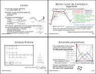
<strong>Exc</strong>. 1: <strong>Hartley</strong> <strong>mixer</strong><br />
<strong>Hartley</strong> <strong>mixer</strong> <strong>cancells</strong> <strong>the</strong> <strong>image</strong> sideband: only signal<br />
will appear in IF port, while <strong>image</strong> is cancelled. This<br />
can be seen using Matlab file hartley.m that convolves<br />
<strong>the</strong> line spectrums given<br />
Do:<br />
• select lower sideband<br />
• select upper sideband<br />
• check <strong>the</strong> effect of 10% error in LO phase shift<br />
<strong>Exc</strong>. 2: AM/AM test<br />
In amam.i AM/AM and AM/PM curves are simulated<br />
using 1-tone harmonic balance<br />
Do:<br />
• Check <strong>the</strong> effect of biasing <strong>the</strong> device in class B or C<br />
by reducing <strong>the</strong> base voltage by 50 mV.<br />
1<br />
2
itest<br />
XIN<br />
RB<br />
(C) 1999- Timo Rahkonen, University of <strong>Oulu</strong>, <strong>Oulu</strong>, Finland<br />
1 1 1 1<br />
4 1 1 4<br />
XOUT<br />
(C) 1999- Timo Rahkonen, University of <strong>Oulu</strong>, <strong>Oulu</strong>, Finland<br />
<strong>Exc</strong>. 3: Measuring Zin<br />
In pierce.i, a CMOS Pierce oscillator is characterized<br />
by driving it by a 1-tone test current source and measuring<br />
<strong>the</strong> voltage that developes across port XOUT-XIN.<br />
Oscillation criteria is that Zamp(Amp) = -Zresonator(f),<br />
so<br />
Find<br />
• excact oscillation amplitude if Re(Zreson) = 18 ohm.<br />
• find Im(Zamp) at that point and note that it will pull<br />
<strong>the</strong> resonance frequency.<br />
Note that due to large RB <strong>the</strong> circuit settles slowly, and<br />
similar amplitude sweep using transient analysis would<br />
be very slow.<br />
<strong>Exc</strong>. 4: Measuring IIP3<br />
In mtanhiip3.i, both conventional and multi-tanh differential<br />
pair are measured using a 2-tone input signal.<br />
The figures are in Chapter 6, when driven from 50 differential<br />
source.<br />
• Run <strong>the</strong> same simulations when driven from 500<br />
ohms<br />
3<br />
4
Maple<br />
.net<br />
rules<br />
Matlab<br />
.mws<br />
function<br />
calls<br />
netlist nli_main<br />
+sweeps<br />
calculation<br />
of<br />
kernels<br />
(C) 1999- Timo Rahkonen, University of <strong>Oulu</strong>, <strong>Oulu</strong>, Finland<br />
voltrules.txt for Maple:<br />
restart;<br />
with(linalg); # initialisation<br />
Maple<br />
Matlab<br />
# nonlin 2nd order current of 1-dim. conductance<br />
# v1,v2 are 1st order voltages at w1, w2<br />
# KV is a vector containing K1,K2,K3<br />
gH2 := proc(v1,v2,KV) ;<br />
KV[2]*v1*v2;<br />
end;<br />
# nonlin 3rd order current of 1-dim. conductance<br />
# v1,v2,v3 are 1st order voltages at w1, w2, w3<br />
# v12, v13,... are 2nd order voltages at w1+w2,<br />
# w1+w3, ...<br />
gH3 := proc(v1,v2,v3,v12,v13,v23,KV) local t1,t2;<br />
t1 := KV[3]*v1*v2*v3;<br />
t2 := 2/3*KV[2]*(v1*v23 + v2*v13 + v3*v12);<br />
evalm(t1+t2); # matrix addition<br />
end;<br />
(C) 1999- Timo Rahkonen, University of <strong>Oulu</strong>, <strong>Oulu</strong>, Finland<br />
VOLTERRA TOOLS<br />
Volterra kernels can be analyzed symbolically using<br />
Maple and numerically using Matlab. In both cases,<br />
<strong>the</strong> following needs to be done:<br />
• describe circuit topology with MNA matrix<br />
• show <strong>the</strong> location of inputs<br />
• list <strong>the</strong> control and output nodes of nonlinear components<br />
Calculation proceeds so that using linear response,<br />
controlling voltages are calculated (in general <strong>the</strong>y are<br />
differential, e.g. v1[3]-v1[4] is voltage between nodes<br />
3 and 4 at frequency w1), and usign <strong>the</strong>m, 2nd order<br />
currents in nonlinear components are calculated (gH2()<br />
and cH2() in Maple).<br />
These currents are now <strong>the</strong> 2nd order input vector for<br />
<strong>the</strong> circuit, and <strong>the</strong>ir voltage response is calculated<br />
using linear model t frequency w1+w2.<br />
Then, using 1st and 2nd order controlling voltages, 3rd<br />
order distortion currents are calculated, injected to <strong>the</strong><br />
circuit and voltage responses are calculated.<br />
# nonlin 2nd order current of a 1-dim cap.<br />
#<br />
cH2 := proc(v1,v2,KV,w1,w2) ;<br />
I*(w1+w2)*KV[2]*v1*v2;<br />
end;<br />
# nonlin 3rd order current of a 1-dim cap.<br />
#<br />
cH3 := proc(v1,v2,v3,v12,v13,v23,KV,w1,w2,w3)<br />
local t1,t2;<br />
t1 := K3*v1*v2*v3;<br />
t2 := 2/3*K2*(v1*v23 + v2*v13 + v3*v12);<br />
I*(w1+w2+w3)*(t1+t2);<br />
end;<br />
5<br />
6
I in 1<br />
(C) 1999- Timo Rahkonen, University of <strong>Oulu</strong>, <strong>Oulu</strong>, Finland<br />
gmramp.net<br />
1<br />
+<br />
-<br />
g mA<br />
## INV AMP: gm loaded by ano<strong>the</strong>r gm and cap<br />
#<br />
# IV: input position, gmXv: K1, K2, K3 of cond. X<br />
#<br />
Iv := vector([ 1, 0]); #linear input signal<br />
gmAv := vector([ gmA, gmA*K2, gmA*K3]);<br />
gmBv := vector([ gmB, gmB*K2, gmB*K3]);<br />
2<br />
C<br />
g mB<br />
# H1 calcs v vector for given current vector input Iin<br />
H1 := proc(w,Iin) local Y;<br />
# MNA admittance matrix<br />
Y := matrix( [<br />
[1, 0 ], # node 1<br />
[gmA , (gmB + I*w*C)] ]); # node 2<br />
evalm( inverse(Y) &* Iin);<br />
end;<br />
H2 := proc(w1,w2)<br />
local v1,v2,inA,inB,H2A,H2B;<br />
v1 := H1(w1,Iv); # 1st order voltage at w1<br />
v2 := H1(w2,Iv); # 1st order voltage at w2<br />
(C) 1999- Timo Rahkonen, University of <strong>Oulu</strong>, <strong>Oulu</strong>, Finland<br />
-<br />
+<br />
<strong>Exc</strong>. 5: Finding Volterra transfer function for amp<br />
In gmramp.net, <strong>the</strong> amplifier on left is described. Current<br />
equations in nodes 1 and 2 are<br />
1 ⋅ v1 = Iin jωC ⋅ v2 = – gmA ⋅ v1 + gmB ⋅ ( – v2) which in matrix form is<br />
1 0 v1 ⋅<br />
gmA ( gmB + jωC ) v2 Next, in voltrules.txt basic rules for Volterra kernels in<br />
Maple are shown, and next, in gmramp.net, <strong>the</strong> circuit<br />
and positions of distortion current sources are shown.<br />
Do:<br />
• derive 2nd order Volterra response<br />
• modify gmramp.net such that <strong>the</strong> control and output<br />
polarity of g mB are changed. It does not affect linear<br />
transfer function but does affect distortion.<br />
# distortion currents and voltages caused by <strong>the</strong>m<br />
inA := gH2(v1[1],v2[1],gmAv); # calc current<br />
H2A := H1(w1+w2,vector([0,-inA]));# inject it<br />
inB := gH2(-v1[2],-v2[2],gmBv);<br />
H2B := H1(w1+w2,vector([0,+inB]));<br />
evalm(H2A + H2B);<br />
end;<br />
H3 := proc(w1,w2,w3)<br />
local v1,v2,v3, v23,v13,v12,inA,inB,H2A,H2B;<br />
v1 := H1(w1,Iv); v2 := H1(w2,Iv); # 1st order<br />
v3 := H1(w3,Iv); v12 := H2(w1,w2);<br />
v13 := H2(w1,w3); v23 := H2(w2,w3); # 2nd ord<br />
# distortion currents and voltages caused by GA,GB<br />
inA :=<br />
gH3(v1[1],v2[1],v3[1],v12[1],v13[1],v23[1],gmAv);<br />
H2A := H1(w1+w2+w3,vector([0,-inA]));<br />
inB := gH3(-v1[2],-v2[2],-v3[2],-v12[2],-v13[2],v23[2],gmBv);<br />
H2B := H1(w1+w2+w3,vector([0,+inB]));<br />
evalm(H2A + H2B);<br />
end;<br />
=<br />
I in<br />
0<br />
7<br />
8
I in<br />
(C) 1999- Timo Rahkonen, University of <strong>Oulu</strong>, <strong>Oulu</strong>, Finland<br />
virtap.net:<br />
+<br />
-<br />
1<br />
-<br />
gmA C gmB go<br />
restart;<br />
with(linalg);<br />
# current mirror<br />
# IV: input position, gmXv: K1, K2, K3 of cond. X<br />
Iv := vector([ 1, 0]);<br />
gmAv := vector([ gmA, gmA*K2, gmA*K3]);<br />
gmBv := vector([ gmB, gmB*K2, gmB*K3]);<br />
# H1: lin. voltage at w with input Iin<br />
H1 := proc(w,Iin) local Y;<br />
#<br />
Y := matrix( [<br />
[(gmA+I*w*C), 0], # node 1<br />
[ gmB , g0] ]); # node 2<br />
evalm( inverse(Y) &* Iin); # solve voltage vect.<br />
end;<br />
H2 := proc(w1,w2)<br />
local v1,v2,inA,inB,H2A,H2B;<br />
v1 := H1(w1,Iv);<br />
v2 := H1(w2,Iv);<br />
(C) 1999- Timo Rahkonen, University of <strong>Oulu</strong>, <strong>Oulu</strong>, Finland<br />
+<br />
2<br />
<strong>Exc</strong>. 6: Finding Volterra for current mirror<br />
In virtap.net, a current mirror on left is described.<br />
Current equations in nodes 1 and 2 are<br />
jωC ⋅ v1 = Iin – gmA ⋅ v1 go ⋅ v2 which in matrix form is<br />
= – gmB ⋅ v1 ( gmA + jωC ) 0<br />
g mB<br />
Its description for Maple is shown on <strong>the</strong> next page.<br />
g o<br />
# distortion currents and voltages caused by <strong>the</strong>m<br />
inA := gH2(v1[1],v2[1],gmAv);<br />
H2A := H1(w1+w2,vector([-inA,0]));<br />
inB := gH2(v1[1],v2[1],gmBv);<br />
H2B := H1(w1+w2,vector([0,-inB]));<br />
evalm(H2A + H2B);<br />
end;<br />
H3 := proc(w1,w2,w3)<br />
local v1,v2,v3, v23,v13,v12,inA,inB,H2A,H2B;<br />
v1 := H1(w1,Iv); v2 := H1(w2,Iv);<br />
v3 := H1(w3,Iv); v12 := H2(w1,w2);<br />
v13 := H2(w1,w3); v23 := H2(w2,w3);<br />
# distortion currs and voltages caused by M1,M2<br />
inA :=<br />
gH3(v1[1],v2[1],v3[1],v12[1],v13[1],v23[1],gmAv);<br />
H2A := H1(w1+w2+w3,vector([-inA,0]));<br />
inB :=<br />
gH3(v1[1],v2[1],v3[1],v12[1],v13[1],v23[1],gmBv);<br />
H2B := H1(w1+w2+w3,vector([0,-inB]));<br />
evalm(H2A + H2B);<br />
end;<br />
⋅<br />
v 1<br />
v 2<br />
=<br />
I in<br />
0<br />
9<br />
10