Data Mining: Concepts and Techniques - LIACS

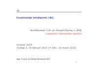
Data Mining: 

Concepts and Techniques 

— Chapter 4 — 

Jiawei Han 

Department of Computer Science 

University of Illinois at Urbana-Champaign 

www.cs.uiuc.edu/~hanj 

©2006 Jiawei Han and Micheline Kamber, All rights reserved 

11/02/10 Data Mining: Concepts and Techniques 1

Sales Data Cube: 

time,item 

A Short Recap on Data Cubes 

Data Cube: A Lattice of Cuboids 

all 

time item location supplier 

time,location 

time,supplier 

time,item,location 

time,item,supplier 

item,location 

time,location,supplier 

time, item, location, supplier 

item,supplier 

item,location,supplier 

location,supplier 

0-D(apex) cuboid 

1-D cuboids 

2-D cuboids 

3-D cuboids 

4-D(base) cuboid 


Multidimensional Data 

Sales volume as a function of product, month, 

and region 

Product Region 

Month 

Dimensions: Product, Location, Time 

Hierarchical summarization paths 

summarize 

Industry Region Year 

Category Country Quarter 

Product City Month Week 

Office Day 


time 

time_key 

day 

day_of_the_week 

month 

quarter 

year 

branch 

branch_key 

branch_name 

branch_type 

Example of Star Schema 

Measures 

Sales Fact Table 

time_key 

item_key 

branch_key 

location_key 

units_sold 

dollars_sold 

avg_sales 

item 

item_key 

item_name 

brand 

type 

supplier_type 

location 

location_key 

street 

city 

state_or_province 

country 


Total sales of TV’s in 1 st quarter in USA 

TV 

PC 

VCR 

sum 

Product 

Total sales in 

USA in 1Qtr 

A Sample Data Cube 

Date 

1Qtr 2Qtr 3Qtr 4Qtr 

2-D Cuboid 

1-D Cuboid 

3-D Cuboid 

sum 

0-D Cuboid 

Total annual sales 

of TV in U.S.A. 

U.S.A 

Canada 

Mexico 

11/02/10 Data Mining: Concepts and Techniques 5 

sum 

Country

Typical OLAP Operations 

Dice 

Slice 

Pivot 

Roll-up 

Drill-down 


Cuboids Corresponding to the Cube 

all 

product date country 

product,date product,country date, country 

product, date, country 


1-D cuboids 

2-D cuboids 



Data Cubes: Ancestor – Descendent relation 

all 

product date country 

product,date product,country date, country 

No Parent/Ancestor – 

Child/Descendant relation! 

Ancestor 

(*,*,*,11540) 

(TV,*,US,300) 

Parent/Ancestor 

product, date, country 

(TV,January,US,45) 

Child/Descendant 

Ancestor 

(*,*,US,1200) 


1-D cuboids 

2-D cuboids 



Chapter 4: Data Cube Computation 

and Data Generalization 

Efficient Computation of Data Cubes 

Exploration and Discovery in Multidimensional 

Databases 

Attribute-Oriented Induction ─ An Alternative 

Data Generalization Method 



Preliminary cube computation tricks (Agarwal et al.’96) 

Computing full/iceberg cubes: 3 methodologies 

Top-Down: Multi-Way array aggregation (Zhao, Deshpande & 

Naughton, SIGMOD’97) 

Bottom-Up: 

Bottom-up computation: BUC (Beyer & Ramarkrishnan, 

SIGMOD’99) 

H-cubing technique (Han, Pei, Dong & Wang: SIGMOD’01) 

Integrating Top-Down and Bottom-Up: 

Star-cubing algorithm (Xin, Han, Li & Wah: VLDB’03) 

High-dimensional OLAP: A Minimal Cubing Approach (Li, et al. 

VLDB’04) 

Computing alternative kinds of cubes: 

Partial cube, closed cube, approximate cube, etc. 


Iceberg Cube 

Computing only the cuboid cells whose 

count or other aggregates satisfying the 

condition like 

Motivation 

HAVING COUNT(*) >= minsup 

Only a small portion of cube cells may be “above the 

water’’ in a sparse cube 

Only calculate “interesting” cells—data above certain 

threshold 

Avoid explosive growth of the cube 

Suppose 100 dimensions, only 1 base cell. How many 

aggregate cells if count >= 1? What about count >= 2? 


Iceberg Cube 

Computing only the cuboid cells whose 

count or other aggregates satisfying the 

condition like 

HAVING COUNT(*) >= minsup 

compute cube sales_iceberg as 

select month, city, customer_group, count(*) 

from salesinfo 

cube by month, city, customer_group 

having count(*) >= minsup 


Closed Cubes 

Database of 100 dimensions has 2 base cells: 

{(a 1 ,a 2 ,a 3 …, a 100 ): 10, (a 1 ,a 2 ,b 3 , …, b 100 ): 10} 

⇒ 2 101 -6 not so interesting aggregate cells: 

{(a 1 ,a 2 ,a 3 ,…,a 99 ,*): 10, (a 1 ,a 2 ,*,a 4 ,…, a 100 ): 10, …, 

(a 1 ,a 2 ,a 3 *,…, *): 10} 

The only 3 interesting aggregate cells would be: 

{(a1 ,a2 ,a3 …, a100 ): 10, {(a1 ,a2 ,b3 …, b100 ): 10, 

(a1 ,a2 ,*, …, *): 20} 


Closed Cubes 

A cell c, is a closed cell, if there exists no cell d 

such that d is a specialization (descendant) of cell 

c (i.e., replacing a * in c with a non-* value), and d has 

the same measure value as c (i.e., d will have strictly 

smaller measure value than c). 

A closed cube is a data cube consisting of only 

closed cells. 

For example the previous three form a lattice of 

closed cells for a closed cube. 


Closed cube lattice: 

Closed Cubes 

(a 1 ,a 2 ,*, …, *): 20 

(a 1 ,a 2 ,a 3 , …, a 100 ): 10 (a1,a2,b 3 , …, b 100 ): 10 


Preliminary Tricks (Agarwal et al. VLDB’96) 

Sorting, hashing, and grouping operations are applied to the dimension 

attributes in order to reorder and cluster related tuples 

Aggregates may be computed from previously computed aggregates, 

rather than from the base fact table 

Smallest-child: computing a cuboid from the smallest, previously 

computed cuboid 

Cache-results: caching results of a cuboid from which other 

cuboids are computed to reduce disk I/Os 

Amortize-scans: computing as many as possible cuboids at the 

same time to amortize disk reads 

Share-sorts: sharing sorting costs cross multiple cuboids when a 

sort-based method is used 

Share-partitions: sharing the partitioning cost across multiple 

cuboids when hash-based algorithms are used 


Multi-Way Array Aggregation 

Array-based “bottom-up” algorithm 

Using multi-dimensional chunks 

No direct tuple comparisons 

Simultaneous aggregation on 

multiple dimensions 

Intermediate aggregate values are 

re-used for computing ancestor 

cuboids 

Cannot do Apriori pruning: No 

iceberg optimization 


all 

A B 

AB 

C 

AC BC 

ABC

B 

Multi-way Array Aggregation for Cube 

Computation (MOLAP) 

Partition arrays into chunks (a small subcube which fits in memory). 

Compressed sparse array addressing: (chunk_id, offset) 

Compute aggregates in “multiway” by visiting cube cells in the order 

which minimizes the # of times to visit each cell, and reduces 

memory access and storage cost. 

C 

c3 61 62 63 64 

c2 45 46 47 48 

c1 

c 0 

29 30 31 32 

b3 B13 

b2 9 

b1 5 

b0 1 

14 

2 

15 

3 

16 

4 

60 

44 

28 

56 

40 

24 

52 

36 

20 

a0 

a1 

A 

a2 a3 

What is the best 

traversing order 

to do multi-way 

aggregation? 


Multi-way Array Aggregation for 

Cube Computation 

B 

C 

c3 61 62 63 64 

c2 45 46 47 48 

c1 

c 0 

29 30 31 32 

b3 

b2 

b1 

b0 

B13 

9 

5 

1 

14 

2 

15 

3 

16 

4 

60 

44 

28 

56 

40 

24 

52 

36 

20 

a0 

a1 

A 

a2 a3 


Multi-way Array Aggregation for 

Cube Computation 

B 

C 

c3 61 62 63 64 

c2 45 46 47 48 

c1 

c 0 

29 30 31 32 

b3 

b2 

b1 

b0 

B13 

9 

5 

1 

14 

2 

15 

3 

16 

4 

60 

44 

28 

56 

40 

24 

52 

36 

20 

a0 

a1 

A 

a2 a3 


Multi-Way Array Aggregation for 

Cube Computation (Cont.) 

Method: the planes should be sorted and computed 

according to their size in ascending order 

Idea: keep the smallest plane in the main memory, 

fetch and compute only one chunk at a time for the 

largest plane 

Limitation of the method: computing well only for a small 

number of dimensions 

If there are a large number of dimensions, “top-down” 

computation and iceberg cube computation methods 

can be explored 


Bottom-Up Computation (BUC) 

BUC (Beyer & Ramakrishnan, 

SIGMOD’99) 

Bottom-up cube computation 

(Note: top-down in our view!) 

Divides dimensions into partitions 

and facilitates iceberg pruning 

If a partition does not satisfy 

min_sup, its descendants can 

be pruned 

If minsup = 1 ⇒ compute full 

CUBE! 

No simultaneous aggregation 

5 ABCD 


AB 

all 

A B C 

AC AD BC BD CD 

ABC ABD ACD BCD 

3 AB 

ABCD 

1 all 

2 A 10 B 14 C 

7 AC 9 AD 11 BC 13 BD 15 CD 

4 ABC 6 ABD 8 ACD 12 BCD 

D 

16 D

BUC: Partitioning 

Usually, entire data set can’t fit in main 

memory 

Sort distinct values, partition into blocks that fit 

Continue processing 

Optimizations 

Partitioning 

External Sorting, Hashing, Counting Sort 

Ordering dimensions to encourage pruning 

Cardinality, Skew, Correlation 

Collapsing duplicates 

Can’t do holistic aggregates anymore! 


H-Cubing: Using H-Tree Structure 

Bottom-up computation 

Exploring an H-tree 

structure 

If the current 

computation of an H-tree 

cannot pass min_sup, do 

not proceed further 

(pruning) 

No simultaneous 

aggregation 


AB 

all 

A B C 

AC AD BC BD CD 

ABC ABD ACD BCD 

ABCD 

D

Header 

table 

Month 

Jan 

Jan 

Jan 

Feb 

Mar 

… 

Attr. Val. 

Edu 

Hhd 

Bus 

… 

Jan 

Feb 

… 

Tor 

Van 

Mon 

… 

City 

Tor 

Tor 

Tor 

Mon 

Van 

… 

H-tree: A Prefix Hyper-tree 

Cust_grp 

Edu 

Hhd 

Edu 

Bus 

Edu 

… 

Quant-Info 

Sum:2285 … 

… 

… 

… 

… 

… 

… 

… 

… 

… 

… 

Prod 

Printer 

TV 

Camera 

Laptop 

HD 

… 

Cost 

500 

800 

1160 

1500 

540 

… 

Side-link 

Price 

485 

1200 

1280 

2500 

520 

… 


bins 

root 

edu hhd bus 

Jan Mar Jan Feb 

Tor Van Tor Mon 

Quant-Info 

Sum: 1765 

Cnt: 2 

Q.I. Q.I. 

Q.I.

H-Cubing: Computing Cells Involving Dimension City 

Header 

Table 

H Tor 

Attr. Val. 

Edu 

Hhd 

Bus 

… 

Jan 

Feb 

… 

Tor 

Van 

Mon 

… 

Attr. Val. 

Edu 

Hhd 

Bus 

… 

Jan 

Feb 

… 

Quant-Info 

Sum:2285 … 

… 

… 

… 

… 

… 

… 

… 

… 

… 

… 

Q.I. 

… 

… 

… 

… 

… 

… 

… 

Side-link 

Side-link 

From (*, *, Tor) to (*, Jan, Tor) 


bins 

root 

Edu. Hhd. Bus. 

Jan. Mar. Jan. Feb. 

Tor. Van. Tor. Mon. 

Quant-Info 

Sum: 1765 

Cnt: 2 

Q.I. Q.I. 

Q.I.

Computing Cells Involving Month But No City 

1. Roll up quant-info 

2. Compute cells involving 

month but no city 

Attr. Val. 

Edu. 

Hhd. 

Bus. 

… 

Jan. 

Feb. 

Mar. 

… 

Tor. 

Van. 

Mont. 

… 

Quant-Info 

Sum:2285 … 

… 

… 

… 

… 

… 

… 

… 

… 

… 

… 

… 

Side-link 


root 

Edu. Hhd. Bus. 

Jan. Mar. Jan. Feb. 

Q.I. 

Q.I. Q.I. 

Q.I. 

Tor. Van. Tor. Mont. 

Top-k OK mark: if Q.I. in a child passes 

top-k avg threshold, so does its parents. 

No binning is needed!

Computing Cells Involving Only Cust_grp 

Check header table directly 

Attr. Val. 

Edu 

Hhd 

Bus 

… 

Jan 

Feb 

Mar 

… 

Tor 

Van 

Mon 

… 

Quant-Info 

Sum:2285 … 

… 

… 

… 

… 

… 

… 

… 

… 

… 

… 

… 

Side-link 


root 

edu hhd bus 

Jan Mar Jan Feb 

Q.I. 

Q.I. Q.I. 

Q.I. 

Tor Van Tor Mon

Star-Cubing: An Integrating Method 

Integrate the top-down and bottom-up methods 

Explore shared dimensions 

E.g., dimension A is the shared dimension of ACD and AD 

ABD/AB means cuboid ABD has shared dimensions AB 

Allows for shared computations 

e.g., cuboid AB is computed simultaneously as ABD 

Aggregate in a top-down manner but with the bottom-up sub-layer 

underneath which will allow Apriori pruning 

Shared dimensions grow in bottom-up fashion 


C/C 

AC/AC AD/A BC/BC BD/B CD 

ABC/ABC ABD/AB ACD/A BCD 

ABCD/all 

D

Iceberg Pruning in Shared Dimensions 

Anti-monotonic property of shared dimensions 

If the measure is anti-monotonic, and if the 

aggregate value on a shared dimension does not 

satisfy the iceberg condition, then all the cells 

extended from this shared dimension cannot 

satisfy the condition either 

Intuition: if we can compute the shared dimensions 

before the actual cuboid, we can use them to do 

Apriori pruning 

Problem: how to prune while still aggregate 

simultaneously on multiple dimensions? 


Use a tree structure similar 

to H-tree to represent 

cuboids 

Collapses common prefixes 

to save memory 

Keep count at node 

Cell Trees 

Traverse the tree to retrieve 

a particular tuple 


Star Attributes and Star Nodes 

Intuition: If a single-dimensional 

aggregate on an attribute value p 

does not satisfy the iceberg 

condition, it is useless to distinguish 

them during the iceberg 

computation 

E.g., b 2 , b 3 , b 4 , c 1 , c 2 , c 4 , d 1 , d 2 , d 3 

Solution: Replace such attributes by 

a *. Such attributes are star 

attributes, and the corresponding 

nodes in the cell tree are star nodes 


A 

a1 

a1 

a1 

a2 

a2 

B 

b1 

b1 

b2 

b3 

b4 

C 

c1 

c4 

c2 

c3 

c3 

D 

d1 

d3 

d2 

d4 

d4 

Count 

1 

1 

1 

1 

1

Suppose minsup = 2 

Example: Star Reduction 

Perform one-dimensional 

aggregation. Replace attribute 

values whose count < 2 with *. And 

collapse all *’s together 

Resulting table has all such 

attributes replaced with the starattribute 

With regards to the iceberg 

computation, this new table is a 

loseless compression of the original 

table 


A 

A 

a1 

a1 

a1 

a2 

a2 

a1 

a1 

a2 

B 

b1 

* 

* 

B 

b1 

b1 

* 

* 

* 

C 

* 

* 

C 

* 

* 

* 

c3 

c3 

c3 

D 

* 

* 

D 

* 

* 

* 

d4 

d4 

d4 

Count 

2 

1 

2 

Count 

1 

1 

1 

1 

1

Given the new compressed 

Star Tree 

table, it is possible to construct 

the corresponding cell tree— 

called star tree 

Keep a star table at the side for 

easy lookup of star attributes 

The star tree is a loseless 

compression of the original cell 

tree 


c*: 14 

Star-Cubing Algorithm—DFS on Lattice Tree 

AB/AB 

BCD: 51 

all 

A/A B/B C/C 

b*: 33 b1: 26 

c3: 211 

c*: 27 

d*: 15 d4: 212 d*: 28 

AC/AC AD/A BC/BC BD/B CD 

ABC/ABC ABD/AB ACD/A BCD 

ABCD 

D/D 

root: 5 

a1: 3 a2: 2 


b*: 1 

c*: 1 

d*: 1 

b1: 2 

c*: 2 

d*: 2 

b*: 2 

c3: 2 

d4: 2

Multi-Way 

Aggregation 

ACD/A 

ABD/AB 

ABC/ABC 


BCD 

ABCD

Star-Cubing Algorithm—DFS on Star-Tree 


Multi-Way Star-Tree Aggregation 

Start depth-first search at the root of the base star tree 

At each new node in the DFS, create corresponding star 

tree that are descendents of the current tree according 

to the integrated traversal ordering 

E.g., in the base tree, when DFS reaches a1, the ACD/ 

A tree is created 

When DFS reaches b*, the ABD/AD tree is created 

The counts in the base tree are carried over to the new 

trees 


Multi-Way Aggregation (2) 

When DFS reaches a leaf node (e.g., d*), start 

backtracking 

On every backtracking branch, the count in the 

corresponding trees are output, the tree is destroyed, 

and the node in the base tree is destroyed 

Example 

When traversing from d* back to c*, the 

a1b*c*/a1b*c* tree is output and destroyed 

When traversing from c* back to b*, the 

a1b*D/a1b* tree is output and destroyed 

When at b*, jump to b1 and repeat similar process 


The Curse of Dimensionality 

None of the previous cubing method can handle high 

dimensionality! 

A database of 600k tuples. Each dimension has 

cardinality of 100 and zipf of 2. 


Motivation of High-D OLAP 

Challenge to current cubing methods: 

The “curse of dimensionality’’ problem 

Iceberg cube and compressed cubes: only delay the 

inevitable explosion 

Full materialization: still significant overhead in 

accessing results on disk 

High-D OLAP is needed in applications 

Science and engineering analysis 

Bio-data analysis: thousands of genes 

Statistical surveys: hundreds of variables 


Fast High-D OLAP with Minimal Cubing 

Observation: OLAP occurs only on a small subset of 

dimensions at a time 

Semi-Online Computational Model 

n Partition the set of dimensions into shell fragments 

n Compute data cubes for each shell fragment while 

retaining inverted indices or value-list indices 

n Given the pre-computed fragment cubes, 

dynamically compute cube cells of the high- 

dimensional data cube online 


Properties of Proposed Method 

Partitions the data vertically 

Reduces high-dimensional cube into a set of lower 

dimensional cubes 

Online re-construction of original high-dimensional space 

Lossless reduction 

Offers tradeoffs between the amount of pre-processing 

and the speed of online computation 


Example Computation 

Let the cube aggregation function be count 

tid 

1 

2 

3 

4 

5 

a2 

b1 

Divide the 5 dimensions into 2 shell fragments: 

(A, B, C) and (D, E) 

A 

a1 

a1 

a1 

a2 

B 

b1 

b2 

b2 

b1 

C 

c1 

c1 

c1 

c1 

c1 


D 

d1 

d2 

d1 

d1 

d1 

E 

e1 

e1 

e2 

e2 

e3

1-D Inverted Indices 

Build traditional inverted index or RID list 

Attribute Value 

a1 

a2 

b1 

b2 

c1 

d1 

d2 

e1 

e2 

e3 

TID List 

1 2 3 

4 5 

1 4 5 

2 3 

1 2 3 4 5 

1 3 4 5 

2 

1 2 

3 4 

5 

List Size 


3 

2 

3 

2 

5 

4 

1 

2 

2 

1

Shell Fragment Cubes 

Generalize the 1-D inverted indices to multi-dimensional 

ones in the data cube sense 

Cell 

a1 b1 

a1 b2 

a2 b1€ 

a2 b2€ 

€ 

€ 

Intersection 

1 2 3 ∩ 1 4 5 

1 2 3 ∩ 2 3 

4 5 ∩ 1 4 5 

4 5 ∩ 2 3 

€ 

TID List 


1 

2 3 

4 5 

⊗ 

List Size 

1 

2 

2 

0

Shell Fragment Cubes (2) 

Compute all cuboids for data cubes ABC and DE while 

retaining the inverted indices 

For example, shell fragment cube ABC contains 7 

cuboids: 

A, B, C 

AB, AC, BC 

ABC 

This completes the offline computation stage 



Given a database of T tuples, D dimensions, and F shell 

fragment size, the fragment cubes’ space requirement is: 

⎛ 

O⎜ 

⎝ 

For F < 5, the growth is sub-linear. 

T 

⎡ 

⎢ 

D 

F 

⎤ 

⎥ 

( 2 

F 


− 

1) 

⎞ 

⎟ 

⎠


Shell fragments do not have to be disjoint 

Fragment groupings can be arbitrary to allow for 

maximum online performance 

Known common combinations (e.g.,) 

should be grouped together. 

Shell fragment sizes can be adjusted for optimal 

balance between offline and online computation 


ID_Measure Table 

If measures other than count are present, store in 

ID_measure table separate from the shell fragments 

tid 

1 

2 

3 

4 

5 

count 

5 

3 

8 

5 

2 

sum 


70 

10 

20 

40 

30

The Frag-Shells Algorithm 

n Partition set of dimension (A 1 ,…,A n ) into a set of k fragments (P 1 , 

…,P k ). 

n Scan base table once and do the following 

n insert into ID_measure table. 

n for each attribute value a i of each dimension A i 

n build inverted index entry 

n For each fragment partition P i 

n build local fragment cube S i by intersecting tid-lists in bottom- 

up fashion. 


A 

B 

ABC 

Cube 

Dimensions 

C 

D 

E 

DEF 

Cube 

Frag-Shells (2) 

F 

… 

D Cuboid 

EF Cuboid 

DE Cuboid 


Cell 

d1 e1 

d1 e2 

d2 e1 

… 

Tuple-ID List 

{1, 3, 8, 9} 

{2, 4, 6, 7} 

{5, 10} 

…

Online Query Computation 

A query has the general form 

Each a i has 3 possible values 

1. Instantiated value 

2. Aggregate * function 

3. Inquire ? function 

For example, 

3 ? ? * 1:count 

returns a 2-D 

data cube. 

€ 

€ 

a 1 ,a 2 ,K,a n : M 


Online Query Computation (2) 

Given the fragment cubes, process a query as 

follows 

n Divide the query into fragment, same as the shell 

n Fetch the corresponding TID list for each 

fragment from the fragment cube 

n Intersect the TID lists from each fragment to 

construct an instantiated base table 

n Compute the data cube using the base table with 

any cubing algorithm 


A 

B 

Online Query Computation (3) 

C 

D 

E 

F 

Instantiated 

Base Table 

G 

H 

I 


J 

K 

L 

M 

Online 

Cube 

N 

…

Experiment: Size vs. Dimensionality 

(cardinality 50 and 100 ) 

(50-C): 10 6 tuples, 0 skew, 50 cardinality, fragment size 3. 

(100-C): 10 6 tuples, 2 skew, 100 cardinality, fragment size 2. 


Experiment: Size vs. Shell-Fragment Size 

(50-D): 10 6 tuples, 50 dimensions, 0 skew, 50 cardinality. 

(100-D): 10 6 tuples, 100 dimensions, 2 skew, 25 cardinality. 


Experiment: Run-time vs. Shell-Fragment 

Size 

10 6 tuples, 20 dimensions, 10 cardinality, skew 1, fragment 

size 3, 3 instantiated dimensions. 


Experiment: I/O vs. Shell-Fragment Size 

(10-D): 10 6 tuples, 10 dimensions, 10 cardinalty, 0 skew, 4 inst., 4 query. 

(20-D): 10 6 tuples, 20 dimensions, 10 cardinalty, 1 skew, 3 inst., 4 query. 


Experiment: I/O vs. # of Instantiated 

Dimensions 

10 6 tuples, 10 dimensions, 10 cardinalty, 0 skew, fragment 

size 1, 7 total relevant dimensions. 


Experiments on Real World Data 

UCI Forest CoverType data set 

54 dimensions, 581K tuples 

Shell fragments of size 2 took 33 seconds and 325MB 

to compute 

3-D subquery with 1 instantiate D: 85ms~1.4 sec. 

Longitudinal Study of Vocational Rehab. Data 

24 dimensions, 8818 tuples 

Shell fragments of size 3 took 0.9 seconds and 60MB 

to compute 

5-D query with 0 instantiated D: 227ms~2.6 sec. 


Comparisons to Related Work 

[Harinarayan96] computes low-dimensional cuboids by 

further aggregation of high-dimensional cuboids. 

Opposite of our method’s direction. 

Inverted indexing structures [Witten99] focus on single 

dimensional data or multi-dimensional data with no 

aggregation. 

Tree-stripping [Berchtold00] uses similar vertical 

partitioning of database but no aggregation. 


Further Implementation Considerations 

Incremental Update: 

Append more TIDs to inverted list 

Add to ID_measure table 

Incremental adding new dimensions 

Form new inverted list and add new fragments 

Bitmap indexing 

May further improve space usage and speed 

Inverted index compression 

Store as d-gaps 

Explore more IR compression methods 










Computing Cubes with Non-Antimonotonic 

Iceberg Conditions 

Most cubing algorithms cannot compute cubes with non- 

antimonotonic iceberg conditions efficiently 

Example 

CREATE CUBE Sales_Iceberg AS 

SELECT month, city, cust_grp, 

AVG(price), COUNT(*) 

FROM Sales_Infor 

CUBEBY month, city, cust_grp 

HAVING AVG(price) >= 800 AND 

COUNT(*) >= 50 

Needs to study how to push constraint into the cubing 

process 


Non-Anti-Monotonic Iceberg Condition 

Anti-monotonic: if a process fails a condition, continue 

processing will still fail 

The cubing query with avg is non-anti-monotonic! 

Month 

Jan 

Jan 

Jan 

Feb 

Mar 

… 

(Mar, *, *, 600, 1800) fails the HAVING clause 

(Mar, *, Bus, 1300, 360) passes the clause 

City 

Tor 

Tor 

Tor 

Mon 

Van 

… 

Cust_grp 

Edu 

Hld 

Edu 

Bus 

Edu 

… 

Prod 

Printer 

TV 

Camera 

Laptop 

HD 

… 

Cost 

500 

800 

1160 

1500 

540 

… 

Price 

485 

1200 

1280 

2500 

520 

… 

CREATE CUBE Sales_Iceberg AS 

SELECT month, city, cust_grp, 

AVG(price), COUNT(*) 

FROM Sales_Infor 

CUBEBY month, city, cust_grp 

HAVING AVG(price) >= 800 AND 

COUNT(*) >= 50 


From Average to Top-k Average 

Let (*, Van, *) cover 1,000 records 

Avg(price) is the average price of those 1000 sales 

Avg 50 (price) is the average price of the top-50 sales 

(top-50 according to the sales price 

Top-k average is anti-monotonic 

The top 50 sales in Van. is with avg(price)

Binning for Top-k Average 

Computing top-k avg is costly with large k 

Binning idea 

Avg 50 (c) >= 800 

Large value collapsing: use a sum and a count to 

summarize records with measure >= 800 

If count>=800, no need to check “small” records 

Small value binning: a group of bins 

One bin covers a range, e.g., 600~800, 400~600, 

etc. 

Register a sum and a count for each bin 


Computing Approximate top-k average 

Suppose for (*, Van, *), we have 

Range 

Over 800 

600~800 

400~600 

… 

Sum 

28000 

10600 

15200 

… 

Count 

20 

15 

30 

… 

Top 50 

Approximate avg 50 ()= 

(28000+10600+600*15)/50=95 

2 

The cell may pass the HAVING clause 

Month 

… 


City 

… 

Cust_grp 

… 

Prod 

… 

Cost 

… 

Price 

…

Weakened Conditions Facilitate Pushing 

Accumulate quant-info for cells to compute average 

iceberg cubes efficiently 

Three pieces: sum, count, top-k bins 

Use top-k bins to estimate/prune descendants 

Use sum and count to consolidate current cell 

weakest 

Approximate avg 50 () 

Anti-monotonic, can 

be computed 

efficiently 

real avg 50 () 

Anti-monotonic, but 

computationally 

costly 

strongest 

avg() 

Not anti- 

monotonic 


Computing Iceberg Cubes with Other 

Complex Measures 

Computing other complex measures 

Key point: find a function which is weaker but ensures 

certain anti-monotonicity 

Examples 

Avg() ≤ v: avg k (c) ≤ v (bottom-k avg) 

Avg() ≥ v only (no count): max(price) ≥ v 

Sum(profit) (profit can be negative): 

p_sum(c) ≥ v if p_count(c) ≥ k; or otherwise, sum k (c) ≥ v 

Others: conjunctions of multiple conditions 


Compressed Cubes: Condensed or Closed Cubes 

W. Wang, H. Lu, J. Feng, J. X. Yu, Condensed Cube: An Effective Approach to 

Reducing Data Cube Size, ICDE’02. 

Icerberg cube cannot solve all the problems 

Suppose 100 dimensions, only 1 base cell with count = 10. How many 

aggregate (non-base) cells if count >= 10? 

Condensed cube 

Only need to store one cell (a 1 , a 2 , …, a 100 , 10), which represents all the 

corresponding aggregate cells 

Adv. 

Fully precomputed cube without compression 

Efficient computation of the minimal condensed cube 

Closed cube 

Dong Xin, Jiawei Han, Zheng Shao, and Hongyan Liu, “C-Cubing: Efficient 

Computation of Closed Cubes by Aggregation-Based Checking”, ICDE'06. 










Discovery-Driven Exploration of Data Cubes 

Hypothesis-driven 

exploration by user, huge search space 

Discovery-driven (Sarawagi, et al.’98) 

Effective navigation of large OLAP data cubes 

pre-compute measures indicating exceptions, guide 

user in the data analysis, at all levels of aggregation 

Exception: significantly different from the value 

anticipated, based on a statistical model 

Visual cues such as background color are used to 

reflect the degree of exception of each cell 


Kinds of Exceptions and their Computation 

Parameters 

SelfExp: surprise of cell relative to other cells at same 

level of aggregation 

InExp: surprise beneath the cell 

PathExp: surprise beneath cell for each drill-down 

path 

Computation of exception indicator (modeling fitting and 

computing SelfExp, InExp, and PathExp values) can be 

overlapped with cube construction 

Exception themselves can be stored, indexed and 

retrieved like precomputed aggregates 


Examples: Discovery-Driven Data Cubes 


Complex Aggregation at Multiple 

Granularities: Multi-Feature Cubes 

Multi-feature cubes (Ross, et al. 1998): Compute complex queries 

involving multiple dependent aggregates at multiple granularities 

Ex. Grouping by all subsets of {item, region, month}, find the 

maximum price in 1997 for each group, and the total sales among all 

maximum price tuples 

select item, region, month, max(price), sum(R.sales) 

from purchases 

where year = 1997 

cube by item, region, month: R 

such that R.price = max(price) 

Continuing the last example, among the max price tuples, find the 

min and max shelf live, and find the fraction of the total sales due to 

tuple that have min shelf life within the set of all max price tuples 


Cube-Gradient (Cubegrade) 

Analysis of changes of sophisticated measures in multi- 

dimensional spaces 

Query: changes of average house price in Vancouver 

in ‘00 comparing against ’99 

Answer: Apts in West went down 20%, houses in 

Metrotown went up 10% 

Cubegrade problem by Imielinski et al. 

Changes in dimensions changes in measures 

Drill-down, roll-up, and mutation 


From Cubegrade to Multi-dimensional 

Constrained Gradients in Data Cubes 

Significantly more expressive than association rules 

Capture trends in user-specified measures 

Serious challenges 

Many trivial cells in a cube “significance constraint” 

to prune trivial cells 

Numerate pairs of cells “probe constraint” to select 

a subset of cells to examine 

Only interesting changes wanted “gradient 

constraint” to capture significant changes 


MD Constrained Gradient Mining 

Significance constraint C sig : (cnt≥100) 

Probe constraint C prb: (city=“Van”, cust_grp=“busi”, 

prod_grp=“*”) 

Gradient constraint C grad (c g , c p ): 

(avg_price(c g)/avg_price(c p)≥1.3) 

Base cell 

Aggregated cell 

Ancestor 

Probe cell: satisfied C prb 

Siblings 

cid 

c1 

c2 

c3 

c4 

Yr 

00 

* 

* 

* 

(c4, c2) satisfies C grad ! 

City 

Van 

Van 

Tor 

* 

Dimensions 

Cst_grp 

58600 


Busi 

Busi 

Busi 

busi 

Prd_grp 

PC 

PC 

PC 

PC 

Cnt 

300 

2800 

7900 

Measures 

Avg_price 

2100 

1800 

2350 

2250

Efficient Computing Cube-gradients 

Compute probe cells using C sig and C prb 

The set of probe cells P is often very small 

Use probe P and constraints to find gradients 

Pushing selection deeply 

Set-oriented processing for probe cells 

Iceberg growing from low to high dimensionalities 

Dynamic pruning probe cells during growth 

Incorporating efficient iceberg cubing method 










What is Concept Description? 

Descriptive vs. predictive data mining 

Descriptive mining: describes concepts or task-relevant 

data sets in concise, summarative, informative, 

discriminative forms 

Predictive mining: Based on data and analysis, 

constructs models for the database, and predicts the 

trend and properties of unknown data 

Concept description: 

Characterization: provides a concise and succinct 

summarization of the given collection of data 

Comparison: provides descriptions comparing two or 

more collections of data 


Data Generalization and Summarization-based 

Characterization 

Data generalization 

A process which abstracts a large set of task-relevant 

data in a database from a low conceptual levels to 

higher ones. 

Approaches: 

Data cube approach(OLAP approach) 

Attribute-oriented induction approach 


1 

2 

3 

4 

5 

Conceptual levels

Similarity: 

Concept Description vs. OLAP 

Data generalization 

Presentation of data summarization at multiple levels of abstraction. 

Interactive drilling, pivoting, slicing and dicing. 

Differences: 

Can handle complex data types of the attributes and their 

aggregations 

Automated desired level allocation. 

Dimension relevance analysis and ranking when there are many 

relevant dimensions. 

Sophisticated typing on dimensions and measures. 

Analytical characterization: data dispersion analysis 


Attribute-Oriented Induction 

Proposed in 1989 (KDD ‘89 workshop) 

Not confined to categorical data nor particular measures 

How it is done? 

Collect the task-relevant data (initial relation) using a 

relational database query 

Perform generalization by attribute removal or 

attribute generalization 

Apply aggregation by merging identical, generalized 

tuples and accumulating their respective counts 

Interactive presentation with users 


Basic Principles of Attribute-Oriented Induction 

Data focusing: task-relevant data, including dimensions, 

and the result is the initial relation 

Attribute-removal: remove attribute A if there is a large set 

of distinct values for A but (1) there is no generalization 

operator on A, or (2) A’s higher level concepts are 

expressed in terms of other attributes 

Attribute-generalization: If there is a large set of distinct 

values for A, and there exists a set of generalization 

operators on A, then select an operator and generalize A 

Attribute-threshold control: typical 2-8, specified/default 

Generalized relation threshold control: control the final 

relation/rule size 


Attribute-Oriented Induction: Basic Algorithm 

InitialRel: Query processing of task-relevant data, deriving 

the initial relation. 

PreGen: Based on the analysis of the number of distinct 

values in each attribute, determine generalization plan for 

each attribute: removal? or how high to generalize? 

PrimeGen: Based on the PreGen plan, perform 

generalization to the right level to derive a “prime 

generalized relation”, accumulating the counts. 

Presentation: User interaction: (1) adjust levels by drilling, 

(2) pivoting, (3) mapping into rules, cross tabs, 

visualization presentations. 


Example 

DMQL: Describe general characteristics of graduate 

students in the Big-University database 

use Big_University_DB 

mine characteristics as “Science_Students” 

in relevance to name, gender, major, birth_place, 

birth_date, residence, phone#, gpa 

from student 

where status in “graduate” 

Corresponding SQL statement: 

Select name, gender, major, birth_place, birth_date, 

residence, phone#, gpa 

from student 

where status in {“Msc”, “MBA”, “PhD” } 


Initial 

Relation 

Prime 

Generalized 

Relation 

Class Characterization: An Example 

Name Gender Major Birth-Place Birth_date Residence Phone # GPA 

Jim M CS Vancouver,BC, 8-12-76 3511 Main St., 687-4598 3.67 

Woodman 

Canada 

Richmond 

Scott M CS Montreal, Que, 28-7-75 345 1st Ave., 253-9106 3.70 

Lachance 

Canada 

Richmond 

Laura Lee 

… 

F 

… 

Physics 

… 

Seattle, WA, USA 

… 

25-8-70 

… 

125 Austin Ave., 

Burnaby 

… 

420-5232 

… 

3.83 

… 

Removed Retained Sci,Eng, 

Bus 

Country Age range City Removed Excl, 

VG,.. 

Gender Major Birth_region Age_range Residence GPA Count 

M Science Canada 20-25 Richmond Very-good 16 

F Science Foreign 25-30 Burnaby Excellent 22 

… … … … … … … 

Gender 

Birth_Region 

Canada Foreign Total 

M 16 14 30 

F 10 22 32 

Total 26 36 62 


Presentation of Generalized Results 

Generalized relation: 

Relations where some or all attributes are generalized, with counts 

or other aggregation values accumulated. 

Cross tabulation: 

Mapping results into cross tabulation form (similar to contingency 

tables). 

Visualization techniques: 

Pie charts, bar charts, curves, cubes, and other visual forms. 

Quantitative characteristic rules: 

Mapping generalized result into characteristic rules with 

quantitative information associated with it, e.g., 

grad( 

x) 

∧ 

male( 

x) 

⇒ 

birth_ 

region( 

x) 

= " Canada" 

[ t: 

53%] 

∨ birth_ 

region( 

x) 

= " foreign" 

[ t: 

47%] 

. 


Mining Class Comparisons 

Comparison: Comparing two or more classes 

Method: 

Partition the set of relevant data into the target class and the 

contrasting class(es) 

Generalize both classes to the same high level concepts 

Compare tuples with the same high level descriptions 

Present for every tuple its description and two measures 

support - distribution within single class 

comparison - distribution between classes 

Highlight the tuples with strong discriminant features 

Relevance Analysis: 

Find attributes (features) which best distinguish different classes 


Quantitative Discriminant Rules 

Cj = target class 

q a = a generalized tuple covers some tuples of class 

but can also cover some tuples of contrasting class 

d-weight 

range: [0, 1] 

− weight = m 

∑ 

i = 1 

quantitative discriminant rule form 

∀ 

d 

X, target_class(X) 

⇐ 

count(q 

condition( X) 


a 

count(q 

∈ 

a 

C 

∈ 

j 

) 

C 

i 

) 

[d : d_weight]

Example: Quantitative Discriminant Rule 

Status Birth_country Age_range Gpa Count 

Graduate Canada 25-30 Good 90 

Undergraduate Canada 25-30 Good 210 

Count distribution between graduate and undergraduate students for a generalized tuple 

Quantitative discriminant rule 

∀ 

X , 

graduate _ student( 

X ) ⇐ 

birth _ country( 

X ) = " Canada" 

∧ age _ range( 

X ) = 

where 90/(90 + 210) = 30% 

30" 

∧ 

gpa( 

X ) = " good" 

: 30%] 


" 25 

− 

[ d

Class Description 

Quantitative characteristic rule 

∀ 

necessary 

Quantitative discriminant rule 

∀ 

sufficient 

Quantitative description rule 

∀ 


⇒ 


⇐ 

X, 

condition 

target_class(X) 

condition( X) 

condition( X) 

⇔ 

(X) [t : w1, 

d : w′ 

1] 

∨ ... ∨ conditionn(X) 

[t : wn, 

d : w n] 

1 ′ 

necessary and sufficient 

[t : t_weight] 

[d : d_weight] 


Example: Quantitative Description Rule 

Location/item TV Computer Both_items 

Count t-wt d-wt Count t-wt d-wt Count t-wt d-wt 

Europe 80 25% 40% 240 75% 30% 320 100% 32% 

N_Am 120 17.65% 60% 560 82.35% 70% 680 100% 68% 

Both_ 

regions 

200 20% 100% 800 80% 100% 1000 100% 100% 

Crosstab showing associated t-weight, d-weight values and total number 

(in thousands) of TVs and computers sold at AllElectronics in 1998 

Quantitative description rule for target class Europe 

∀ 

X, Europe(X) 

(item(X) = " TV" 

⇔ 

) [t : 25%, d : 40%] ∨ (item(X) = " computer" ) [t 

: 75%, d 

: 30%] 


Summary 

Efficient algorithms for computing data cubes 

Multiway array aggregation 

BUC 

H-cubing 

Star-cubing 

High-D OLAP by minimal cubing 

Further development of data cube technology 

Discovery-drive cube 

Multi-feature cubes 

Cube-gradient analysis 

Anther generalization approach: Attribute-Oriented Induction 


References (I) 

S. Agarwal, R. Agrawal, P. M. Deshpande, A. Gupta, J. F. Naughton, R. Ramakrishnan, 

and S. Sarawagi. On the computation of multidimensional aggregates. VLDB’96 

D. Agrawal, A. E. Abbadi, A. Singh, and T. Yurek. Efficient view maintenance in data 

warehouses. SIGMOD’97 

R. Agrawal, A. Gupta, and S. Sarawagi. Modeling multidimensional databases. ICDE’97 

K. Beyer and R. Ramakrishnan. Bottom-Up Computation of Sparse and Iceberg CUBEs.. 

SIGMOD’99 

Y. Chen, G. Dong, J. Han, B. W. Wah, and J. Wang, Multi-Dimensional Regression 

Analysis of Time-Series Data Streams, VLDB'02 

G. Dong, J. Han, J. Lam, J. Pei, K. Wang. Mining Multi-dimensional Constrained Gradients 

in Data Cubes. VLDB’ 01 

J. Han, Y. Cai and N. Cercone, Knowledge Discovery in Databases: An Attribute-Oriented 

Approach, VLDB'92 

J. Han, J. Pei, G. Dong, K. Wang. Efficient Computation of Iceberg Cubes With Complex 

Measures. SIGMOD’01 


References (II) 

L. V. S. Lakshmanan, J. Pei, and J. Han, Quotient Cube: How to Summarize the 

Semantics of a Data Cube, VLDB'02 

X. Li, J. Han, and H. Gonzalez, High-Dimensional OLAP: A Minimal Cubing Approach, 

VLDB'04 

K. Ross and D. Srivastava. Fast computation of sparse datacubes. VLDB’97 

K. A. Ross, D. Srivastava, and D. Chatziantoniou. Complex aggregation at multiple 

granularities. EDBT'98 

S. Sarawagi, R. Agrawal, and N. Megiddo. Discovery-driven exploration of OLAP data 

cubes. EDBT'98 

G. Sathe and S. Sarawagi. Intelligent Rollups in Multidimensional OLAP Data. VLDB'01 

D. Xin, J. Han, X. Li, B. W. Wah, Star-Cubing: Computing Iceberg Cubes by Top-Down 

and Bottom-Up Integration, VLDB'03 

D. Xin, J. Han, Z. Shao, H. Liu, C-Cubing: Efficient Computation of Closed Cubes by 

Aggregation-Based Checking, ICDE'06 

W. Wang, H. Lu, J. Feng, J. X. Yu, Condensed Cube: An Effective Approach to Reducing 

Data Cube Size. ICDE’02 

Y. Zhao, P. M. Deshpande, and J. F. Naughton. An array-based algorithm for 

simultaneous multidimensional aggregates. SIGMOD’97 


SQL Group By statement 

From: http://www.w3schools.com/sql/sql_groupby.asp

Data Mining: Concepts and Techniques - LIACS

You also want an ePaper? Increase the reach of your titles

Delete template?

Save as template?