Math 257 and 316 Partial Differential Equations - UBC Math

Math 257 and 316
Partial Differential Equations
c○1999 Richard Froese. Permission is granted to make and distribute verbatim copies of this document provided
the copyright notice and this permission notice are preserved on all copies.

Math 257 and 316 1
Introduction
This is a course about partial differential equations, or PDE’s. These are differential equations involving partial
derivatives and multi-variable functions.
An example: temperature flow
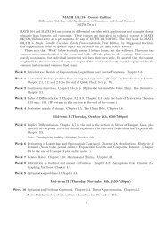
Consider the following experiment. A copper cube (with side length 10cm) is taken from a refrigerator (at
temperature −4 ◦ ) and, at time t =0is placed in a large pot of boiling water. What is the temperature of the
centre of the cube after 60 seconds?
z
Introduce the x, y and z co-ordinate axes, with the origin located at one corner of the cube as shown. Let
T (x, y, z, t) be the temperature of the point (x, y, z) inside the cube at time t. Then T (x, y, z, t) is defined for all
(x, y, z) inside the cube (i.e., 0 ≤ x, y, z ≤ 10), and all t ≥ 0. Our goal is to determine the function T , in particular,
to find T (5, 5, 5, 100).
There are three facts about T (x, y, z, t) that are needed to determine it completely. Firstly, T solves the partial
differential equation governing heat flow, called the heat equation. This means that for every (x, y, z) in the cube
and every t>0,
∂T
∂t
= α2
y
2 ∂ T
∂x2 + ∂2T ∂y2 + ∂2T ∂z2
Here α 2 is a constant called the thermal diffusivity. This constant depends on what kind of metal the cube is
made of. For copper α 2 =1.14 cm 2 /sec
The second fact about T is that it satisfies a boundary condition. We assume that the pot of water is so large that
the temperature of the water is not affected by the insertion of the cube. This means that the boundary of the
cube is always held at the constant temperature 100 ◦ . In other words
T (x, y, z, t) = 100 for all (x, y, z) on the boundary of the cube and all t>0.
The third fact about T is that it satisfies an initial condition. At time t =0the cube is at a uniform temperature
of −4 ◦ . This means that
T (x, y, z, 0) = −4 for all (x, y, z) inside the cube.
x

2 Math 257 and 316
Given these three facts we can determine T completely. In this course we will learn how to write down the
solution in the form of an infinite (Fourier) series. For now I’ll just write down the answer.
where
and
T (x, y, z, t) = 100 +
∞
∞
n=1 m=1 l=1
an,m,l = −104
∞
an,m,le −α2λm,n,lt sin(nπx/10) sin(mπy/10) sin(lπz/10)
λm,n,l =(π/10) 2 (n 2 + m 2 + l 2 )
3 2 1
π nml (1 − (−1)n )(1 − (−1) m )(1 − (−1) l )
Problem 1.1: What temperature does the formula above predict for the centre of the cube at time t =60
if you use just one term ((n, m, l) =(1, 1, 1)) in the sum. What is the answer if you include the terms
(n, m, l) =(1, 1, 1), (3, 1, 1), (1, 3, 1), (1, 1, 3)?
Basic equations
The three basic equations that we will consider in this course are the heat equation, the wave equation and
Laplace’s equation. We have already seen the heat equation in the section above. The sum of the second partial
derivatives with repsect to the space variables (x, y and z) is given a special name—the Laplacian or the Laplace
operator—and is denoted ∆. Thus the Laplacian of u is denoted
With this notation the heat equation can be written
∆u = ∂2u ∂x2 + ∂2u ∂y2 + ∂2u ∂z2 ∂u
∂t = α2 ∆u (1.1)
Sometimes we are interested in situations where there are fewer than three space variables. For example, if we
want to describe heat flow in a thin plate that is insulated on the top and the bottom, then the temperature
function only depends on two space variables, x and y. The heat flow in a thin insulated rod would be described
by a function depending on only one space variable x. In these situations we redefine ∆ to mean
or
∆u = ∂2u ∂x2 + ∂2u ∂y2 ∆u = ∂2 u
∂x 2
depending on the context. The heat equation is then still written in the form (1.1).
The second basic equation is the wave equation
∂ 2 u
∂t 2 = c2 ∆u

Math 257 and 316 3
This equation decribes a vibrating string (one space dimension) a vibrating drum or water waves (two space
dimensions) or an electric field propagating in free space (three space dimensions).
The third basic equation is the Laplace equation
∆u =0
Notice that a solution of Laplace’s equation can be considered to be a solution of the wave or heat equation
that is constant in time (so that ∂u/∂t = ∂ 2 u/∂t 2 =0). So we see that solutions to Laplace’s equation describe
equilibrium situations. For example, the temperature distrubution after a long time a passed, or the electric field
produced by stationary charges are solutions of Laplace’s equation.
These are all second order equations because there are at most two derivatives applied to the unknown function.
These equations are also all linear. This means that if u1(x, y, z, t) and u2(x, y, z, t) are solutions then so is the
linear combination a1u1(x, y, z, t)+a2u2(x, y, z, t). This fact is sometimes called the superpostion principle. For
example, if u1 and u2 both satisfy the heat equation, then
∂
∂t (a1u1
∂u1 ∂u2
+ a2u2) =a1 + a2
∂t ∂t
= a1α 2 ∆u1 + a2α 2 ∆u2
= α 2 ∆(a1u1 + a2u2)
Thus the linear combination a1u1 + a2u2 solves the heat equation too. This reasoning can be extended to a linear
combination of any number, even infinitely many, solutions.
Here is how the superposition principle is applied in practice. We try to get a good supply of basic solutions
that satisfy the equation, but not neccesarily the desired boundary condition or the initial condition. These basic
solutions are obtained by a technique called separation of variables. Then we try to form a (possibly infinite)
linear combination of the basic solutions in such a way that the initial condition and boundary condition are
satisfied as well.
Problem 1.2: Show that for each fixed n, m and l the function
e −α2 λm,n,lt sin(nπx/10) sin(mπx/10) sin(lπx/10)
is a solution of the heat equation. What is the boundary condition satisfied by these functions? Is this boundary
condition preserved when we form a linear combination of these functions? Notice that the solution T above
is an infinite linear combination of these functions, together with constant function 100.
Problem 1.3: What is the limiting temperature distribution in the example as t →∞? Show that is an
(admitedly pretty trivial) solution of the Laplace equation.
Problem 1.4: When there is only one space variable, then Laplace’s equation is the ordinary differential
equation u ′′ =0rather than a partial differential equation. Write down all possible solutions.
If you have taken a course in complex analysis, you will know that the real part (and the imaginary part) of
every analytic function is a solution to Laplace’s equation in two variables. Thus there are many more solutions
to Laplace’s equations when it is a PDE.

4 Math 257 and 316
What else is in this course?
The series arising in the solutions of the basic equations are often Fourier series. Fourier series are of independent
interest, and we will devote some time at the beginning of this course studying them.
Fourier series expansions can be considered as special cases of expansions in eigenfunctions of Sturm-Liouville
problems. More general Sturm-Liouville expansions arise when considering slighly more complicated (and
realistic) versions of the basic equations, or when using non-Cartesian co-ordinate systems, such as polar coordinates.
We will therefore spend some time looking at Sturm-Liouville problems.

Math 257 and 316 5
Fourier series
Consider a function f(x) of one variable that is periodic with period L. This means that f(x + L) =f(x) for
every x. Here is a picture of such a function.
L 2L 3L
Such a function is completely determined by its values on any interval of length L, for example [0,L] or
[−L/2,L/2]. If we start with any function defined on an interval of length L, say [0,L],
L 2L 3L
we can extend it to be a periodic function by simply repeating its values.
L 2L 3L
Notice, however, that the periodic extention will most likely have a jump at the points where it is glued together,
and not be a continuous function.
The Fourier series for f is an infinite series expansion of the form
f(x) = a0
2 +
∞
an cos(2πnx/L)+bn sin(2πnx/L)
n=1
Each function appearing on the right side—the constant function 1, the functions cos(2πnx/L) and the functions
sin(2πnx/L) for n =1, 2, 3,...—are all periodic with period L. Apart form this, though, there is not any apparent
reason why such an expansion should be possible.
For the moment, we will just assume that it is possible to make such an expansion, and try to determine what
the coefficients an and bn must be. The basis for this determination are the following integral formulas, called
orthogonality relations.
L
L
cos(2πnx/L)dx = sin(2πnx/L)dx =0 for every n (2.2)
0
0

6 Math 257 and 316
L
cos(2πnx/L)sin(2πmx/L)dx =0 for every n and m (2.3)
0
L
sin(2πnx/L)sin(2πmx/L)dx =
0
L
cos(2πnx/L)cos(2πmx/L)dx =
0
L/2 if n = m
0 otherwise
L/2 if n = m
0 otherwise
Notice that we can change L
0 to L/2
−L/2 (or to the integral over any other interval of length L) without changing
the values of the integrals. This can be seen geometrically: the area under the curve of a periodic function between
x = L/2 and x = L is the same as the area under the curve between −L/2 and x =0, so we can shift that part of
the integral over.
If we want to determine am (for m ≥ 1) we first multiply both sides of (2.1) by cos(2πmx/L) and integrate. This
gives
L
cos(2πmx/L)f(x)dx =
0
a0
L
cos(2πmx/L)dx+
2 0
L ∞
an cos(2πmx/L)cos(2πnx/L)+bn cos(2πmx/L)sin(2πnx/L) dx
0
n=1
Now we change the order of summation and integration. This is not always justfied (i.e., summing first and then
integrating could give a different answer than integrating first and then summing). However, at the moment, we
don’t really even know that the Fourier series converges, and are just trying to come up with some formula for
am. So we will go ahead and make the exchange, obtaining
L
cos(2πmx/L)f(x)dx =
0
a0
L
cos(2πmx/L)dx+
2 0
∞
L
L
an cos(2πmx/L)cos(2πnx/L)dx + bn cos(2πmx/L) sin(2πnx/L)dx
n=1
0
Using the orthogonality realtions, we see that all the terms are zero except the one with n = m. Thus
so that
L
L
cos(2πmx/L)f(x)dx = am cos 2 (2πmx/L)dx = amL/2
0
am = 2
L
0
L
cos(2πmx/L)f(x)dx.
0
Similary, multiplying (2.1) by sin(2πmx/L), integrating, changing the order of summation and integration, and
using the orthogonality relations, we obtain
bm = 2
L
L
sin(2πmx/L)f(x)dx.
0
Finally, if we multiply (2.1) by 1 (which does nothing, of course) and follow the same steps we get
a0 = 2
L
L
f(x)dx
0
0
(2.4)
(2.5)

Math 257 and 316 7
(This can also be written 2/L L
0 cos(2π0x/L)f(x)dx, and agrees with the formula for the other am’s. This is the
reason for the factor of 1/2 in the a0/2 term in the original expression for the Fourier series.)
Examples
Given a periodic function f (or a function on [0,L] which we extend periodically) we now have formulas for the
coefficients an and bn in the fourier expansion. We can therefore compute all the terms in the fourier expansion,
and see if it approximates the original function.
Lets try this for a triangular wave defined on [0, 1] by
x if 0 ≤ x ≤ 1/2
f(x) =
1 − x if 1/2 ≤ x ≤ 1
1
0 1
In this example L =1. Using the formulas from the last section we have
a0 =2
1
0
f(x)dx =1/2
(since the area under the triangle is 1/4). For n ≥ 1 we obtain (after some integration by parts)
an =2
=2
1
0
1/2
cos(2πnx)f(x)dx
1
cos(2πnx)xdx +2 cos(2πnx)(1 − x)dx
1/2
0
=((−1) n − 1)/(π 2 n 2 )
=
0 if n is even
−2/(π 2 n 2 ) if n is odd
and
1
bn =2 sin(2πnx)f(x)dx
0
1/2
1
=2 sin(2πnx)xdx +2 sin(2πnx)(1 − x)dx
0
1/2
=0
Thus, if the Fourier series for f(x) really does converge to f(x) we have,
f(x) = 1
− 2
4
= 1
4
− 2
∞
n=1
nodd
∞
n=0
1
π2 cos(2πnx)
n2 1
π2 cos(2π(2n +1)x)
(2n +1) 2

8 Math 257 and 316
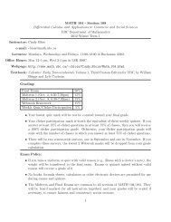
Does the series converge to f? We can try to look at the partial sums and see how good the approximation is.
Here is a graph of the first 2, 3 and 7 non-zero terms.
0.4
0.3
0.2
0.1
–1 –0.8 –0.6 –0.4 –0.2 0 0.2 0.4 0.6 0.8 1 1.2 1.4 1.6 1.8 2
x
2 non zero terms
0.4
0.3
0.2
0.1
–1 –0.8 –0.6 –0.4 –0.2 0 0.2 0.4 0.6 0.8 1 1.2 1.4 1.6 1.8 2
x
3 non zero terms
0.5
0.4
0.3
0.2
0.1
–1 –0.8 –0.6 –0.4 –0.2 0 0.2 0.4 0.6 0.8 1 1.2 1.4 1.6 1.8 2
x
7 non zero terms
It looks like the series is converging very quickly indeed.
Lets try another example. This time we take L =2and f(x) to be a square wave given by
f(x) =
1
1 if 0 ≤ x

an = 2
2
Math 257 and 316 9
=
=0
2
0
1
0
bn = 2
2
=
cos((2πnx)/2)f(x)dx
cos(πnx)dx
2
0
1
Thus, if the series for this f exists, it is given by
f(x) = 1
2 +
0
sin((2πnx)/2)f(x)dx
sin(πnx)dx
=(1− (−1) n )/(πn)
0 if n is even
=
2/(πn) if n is odd
= 1
2 +
∞
n=1
nodd
∞
n=0
2
πn sin(πnx)
2
sin(π(2n +1)x)
π(2n +1)
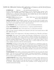
Here are the graphs of the first 2, 3, 7 and 20 non-zero terms in the series.
1
0.8
0.6
0.4
0.2
–2 –1 0
1 2 3 4 5
x
2 non zero terms
1
0.8
0.6
0.4
0.2
–2 –1 0
1 2 3 4 5
x
3 non zero terms
1
0.8
0.6
0.4
0.2
–2 –1 0
1 2 3 4 5
x
7 non zero terms

10 Math 257 and 316
1
0.8
0.6
0.4
0.2
–2 –1 0
1 2 3 4 5
x
20 non zero terms
The series seems to be converging, although the convergence doesn’t seem so good near the discontinuities.
The fact that there is a bump near the discontinuity is called Gibb’s phenonemon. The bump moves closer and
closer to the point of discontinuity as more and more terms in the series are taken. So for any fixed x, the bump
eventually passes by. But it never quite goes away. (For those of you who know about uniform convergence: this
is an example of a series that converges pointwise but not uniformly.)
Problem 2.1: Compute the coefficents an and bn when L =1and
f(x) =
1 if 0 ≤ x ≤ 1/2
−1 if 1/2

Math 257 and 316 11
1
0
x0x11 Theorem 2.2 Suppose that f(x) is a periodic function with period L, and that both f and its derivative f ′
are piecewise continuous on each interval of length L. Then at all points of continuity x the Fourier series
evaluated at x converges to f(x). At the finitely many points of discontinuity xk, the Fourier series evaluated
at xk converges to the average of the limits from the right and the left of f, i.e., to (f(xk+) + f(xk−))/2.
Although we won’t be able to prove this theorem in this course, here is some idea how one would go about it.
Let Fn(x) be the partial sum
Fm(x) = a0
2 +
m
an cos(2πnx/L)+bn sin(2πnx/L)
n=1
Our goal would be to show that Fm(x) → f(x) as m →∞. If we substitute the formulas for an and bn we get
Fm(x) = 1
L
2
f(y)dy
2 L 0
m
L
L
2
2
+
cos(2πmy/L)f(y)dy cos(2πnx/L)+ sin(2πmy/L)f(y)dy sin(2πnx/L)
L
n=1 0
L 0
L
m
1 2
= + cos(2πmx/L)cos(2πny/L) + sin(2πmx/L)sin(2πny/L) f(y)dy
0 L L
n=1
L
m
1 2
= + cos(2πm(x − y)/L) f(y)dy
0 L L
n=1
L
= Km(x − y)f(y)dy
where
0
Km(x − y) = 1 2
+
L L
m
cos(2πm(x − y)/L)
n=1
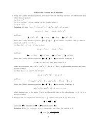
to understand why Fm(x) should converge to f(x) we have to examine the function Km(x − y). Here is a picture
(with m =20, x =0and L =1).
40
30
20
10
–0.4 –0.2 0
0.2 0.4
x

12 Math 257 and 316
Notice that there is a big spike when y is close to x. The area under this spike is approximately 1. For values of y
away from x, the function is oscillating. When m gets large, the spike get concentrated closer and closer to x and
the the oscillations get more and more wild. So
L
Km(x − y)f(y)dy =
y close to x
0
Km(x − y)f(y)dy +
Km(x − y)f(y)dy
y far from x
When m is very large we can restrict the first integral over y values that are so close to x that f(y) is essentially
equal to f(x). Then we have
Km(x − y)f(y)dy ∼
y close to x
Km(x − y)f(x)dy = f(x)
y close to x
Km(x − y)dy ∼ f(x)
y close to x
because the area under the spike is about 1. On the other hand
Km(x − y)f(y)dy ∼ 0
y far from x
for large m since the wild oscillations tend to cancel out in the integral. To make these ideas exact, one needs to
assume more about the function f, for example, the assumptions made in the theorems above.
Complex form
We will now the Fourier series in complex exponential form.
f(x) =
∞
n=−∞
(To simplify the formulas, we will assume that L =1in this section.) Recall that
Therefore
e it =cos(t)+i sin(t).
cne i2πnx . (2.6)
cos(t) = eit + e−it 2
sin(t) = eit − e−it .
2i
To obtain the complex exponential form of the fourier series we simply substitute these expressions into the
original series. This gives
where
f(x) = a0
2 +
= a0
2 +
=
∞
n=−∞
∞
n=1
an
2
∞
an n=1
2
cne i2πnx
i2πnx −i2πnx
e + e + bn
i2πnx −i2πnx
e − e
2i
c0 = a0
2
cn = an
2
cn = a−n
2
bn
+ e
2i
i2πnx
an
+
2
+ bn
2i
− b−n
2i
for n>0
for n

Math 257 and 316 13
This complex form of the Fourier series is completely equivalent to the original series. Given the an’s and bn’s
we can compute the cn’s using the formula above, and conversely, given the cn’s we can solve for
a0 =2c0
an = cn + c−n for n>0
bn = icn − ic−n for n>0
It is actually often easier to compute the cn’s directly. To do this we need the appropriate orthogonality relations
for the functions e i2πnx . They are
1
0
e −i2πmx e i2πnx dx =
1
0
e i2π(n−m)x dx =
0 if n = m
1 if n = m
So to pick out the coefficient cm in the complex Fourier series, we multiply (2.6) by e −i2πmx and integrate. This
gives (after exchanging the integral and the infinite sum)
1
0
e −i2πmx f(x)dx =
∞
n=−∞
cn
1
0
e −i2πmx e i2πnx dx = cm
Lets compute the complex Fourier series coefficients for the square wave function
1 if 0 ≤ x ≤ 1/2
f(x) =
−1 if 1/2

14 Math 257 and 316
Problem 2.3: Calculate the formula for the cn’s when L is different from 1. Use your formula to compute
the coefficents cn when L =2and
f(x) =x if 0 ≤ x ≤ 2
Calculate an and bn from your expression for the cn and compare to the result obtained in a previous problem.
Even and Odd functions
A function f(x) is called even if f(−x) =f(x) and odd if f(x) =−f(−x) Here is are picture of an even function
and an odd function.
f(x)
x
If we multiply together two even functions or two odd functions, the result is an even function. If we multiply
together and odd and an even function, the result is an odd function.
The integral of an odd function over an interval that is symmetric with respect to the origin is zero. This can be
seen geometrically:
f(x)
B
A
-a
-A
-B
a
The integral from −a to a of this odd function is zero, since the positive areas on one side of the origin cancel the
negative ones on the other side. Similarly, the integral from −a to a of an even function is just twice the integral
of the same function. Thus
a
a
a
odd(x)dx =0 even(x)dx =2 even(x)dx
−a
−a
0
These ideas can be applied to the calculation of Fourier coefficients because cos(2πnx/L) is an even function (for
every n) and sin(2πnx/L) is an odd function (for every n). Recall that the interval of integration appearing in the
definition of an and bncan be any interval of length L. Before we chose [0,L]. But now, to apply the formulas for
odd and even functions we want an interval that is symmetric about zero. So we choose [−L/2,L/2] and write
an = 2
L
bn = 2
L
x
f(x)
L/2
cos(2πnx/L)f(x)dx,
−L/2
L/2
sin(2πnx/L)f(x)dx.
−L/2
x

Math 257 and 316 15
If f(x) is even, then cos(2πnx/L)f(x) is also even and sin(2πnx/L)f(x) is odd. Thus
an = 4
L/2
cos(2πnx/L)f(x)dx,
L 0
bn =0.
If f(x) is odd, then cos(2πnx/L)f(x) is odd and sin(2πnx/L)f(x) is even. Thus
Example
4
L
L/2
sin(2πnx/L)f(x)dx.
0
an =0,
bn =
Let us compute the Fourier coeffients of the function f(x) with period L =2given by
⎧
⎨ −1 − x if −1 ≤ x ≤−1/2
f(x) = x
⎩
1 − x
if −1/2 ≤ x ≤ 1/2
if 1/2 ≤ x ≤ 1
Here is a picture of f.
Notice that f is odd. Thus an =0for every n and
bn = 4
2
=2
1
0
1/2
-1
sin(2πnx/2)f(x)dx
1
sin(πnx)xdx +2 sin(πnx)(1 − x)dx
1/2
0
=4sin(nπ/2)/(π 2 n 2 )
Problem 2.4: Find the Fourier coefficients of the function with period L =4given by
0 if −2 ≤ x

16 Math 257 and 316
Problem 2.6: Suppose f and g are odd and even functions that have been shifted vertically, i.e., f(x) =
C + odd(x) and g(x) =C +even(x), whereC is a constant. Which Fourier coefficients are zero?
Problem 2.7: Suppose that L =1and f(x) is odd with respect to 1/2, i.e., f(1/2+x) =f(1/2 − x)
for every x. What can you say about the Fourier coefficients of f ?
Sine and Cosine series
Suppose we are given two different periodic functions, with possibly different periods. Suppose, though, that
these two functions happen to agree on some interval. Then the Fourier series for the two functions will be
different. In fact, if the periods are different then there will be completely different set of sine and cosine functions
appearing in the two expansions. Nevertheless, in the interval where the two functions agree, the two Fourier
expansions will converge to the same thing.
We will use this observation, together with the facts about odd and even functions, to produce a variety of
expansions for the same function.
We begin with a function defined on the interval [0, 1]. For definiteness, take f(x) =x.
We can extend this function to be periodic with period 1 and expand in a Fourier series. The formulas for the
coefficients are
an = 2
1
1 if n =0
cos(2πnx)xdx =
1 0
0 if n>1
bn = 2
1
sin(2πnx)xdx = −1/(πn)
1
and the series
a0
2 +
∞
n=1
0
an cos(2πnx)+bn sin(2πnx) = 1
2 −
∞
n=1
1
sin(2πnx) (2.7)
πn
converges to a periodic function of period 1 that agrees with f(x) =x on [0, 1] (except right at the discontinuity,
where the Fourier series converges to 1/2). Here is a picture of the Fourier series.
Next, we will start with the same function f(x) =x on the interval [0, 1], but first extend it to be an odd function
on [−1, 1], and then extend it to be a periodic function of period L =2. The complete extension looks like

Math 257 and 316 17
What is the Fourier series for this function. Well, now L =2and the function is odd. So all the an’s are zero, and
So the series is
bn = 4
2
n=1
1
0
sin(nπx)xdx =2(−1) n+1 /(πn)
∞
∞ 2(−1)
bn sin(πnx) =
n+1
sin(nπx) (2.8)
πn
n=1
This is called the sine series for f. It converges to the periodic function with period L =2depicted above (except
for the points of discontinuity, where it converges to the midpoint).
Finally, we start again with the same function f(x) =x on the interval [0, 1], extend it to be an even function on
[−1, 1], and then extend it to be a periodic function of period L =2. The complete extension now looks like
This is an even function with L =2. So all the bn’s are now zero, while the an’s are given by
Therefore the series
4
2
1
0
a0
2 +
cos(πnx)xdx =
∞
n=1
an cos(πnx) = 1
2 +
1 if n =0
2((−1) n − 1)/(π 2 n 2 ) if n ≥ 1
∞
n=1
2 (−1)n − 1
π 2 n 2 cos(πnx) (2.9)
converges to the periodic function depicted above. This is called the cosine series.
If we restrict our attention to values of x in the interval [0, 1] we have produced three different expansions for the
same function, namely (2.7), (2.8) and (2.9). (One could produce even more, by making different extensions.) We
will see that all these series are useful in solving PDE’s.
Problem 2.8: Which of the expansions (2.7), (2.8), (2.9) converges the fastest? Which of the resulting periodic
functions are continuous?
Problem 2.9: Compute the sine and cosine series for
1 if 0 ≤ x ≤ 1/2
f(x) =
−1 if 1/2

18 Math 257 and 316
Infinite orthogonal bases
Lets write down functions appearing on the right side of the expansions of the previous section. We have
for (2.7),
for (2.8) and
for (2.9). We could also add the set
{ 1
, cos(2πx), cos(4πx), cos(6πx),...sin(2πx), sin(4πx), sin(6πx),...}
2
{sin(πx), sin(2πx), sin(3πx),...}
{ 1
, cos(πx), cos(2πx), cos(3πx),...}
2
{...,e −4iπx ,e −2iπx ,e 0iπx ,e 2iπx ,e 4iπx ,...}
for the complex Fourier series.
We can think of these lists of functions {φ1(x),φ2(x),φ3(x),...} as infinite bases in a vector space of functions.
A given function f(x) on the interval [0, 1] can be expanded in an infinite sum
f(x) =
aiφi(x)
i
for each of these sets. This is analgous to expanding a given vector with respect to various bases in a vector space.
To understand this analogy, think back to your last linear algebra course. A collection of vectors in a vector space
form a basis if they span the space (that is, every vector can be written as a linear combination of basis vectors)
and are linearly independent (that is, there is exaclty one way to write this linear combination). Three non-zero
vectors {v1, v2, v3} in three dimensional space form a basis if they don’t all lie in the same plane. In this case an
arbitrary vector v can be expanded in a unique way as a linear combination
v = a1v1 + a2v2 + a3v3
However, for a general basis, its not that easy to find the coefficients, a1, a2 and a3. Finding them requires solving
a system of linear equations.
Things are much easier if the basis is an orthogonal basis. This means that the inner (dot) product 〈vi, vj〉 is zero
if i = j. In this case we can find the coefficients ai by taking inner products. For example, to find a1, we take the
inner product with v1. This gives
Thus
〈v1, v〉 = a1〈v1, v1〉 + a2〈v1, v2〉 + a3〈v1, v3〉
= a1〈v1, v1〉 +0+0
a1 = 〈v1, v〉/〈v1, v1〉
The sets of functions above can be thought of as infinite orthogonal bases for a vector space of functions. (I’m
being a bit vague on exactly what functions are allowed, certainly all functions that are piecewise continuous
with continuous derivative are included.)
What is the inner product of two functions f(x) and g(x)? It is given by the integral
〈f,g〉 =
1
0
¯f(x)g(x)dx

Math 257 and 316 19
(The complex conjugate ¯ f is only relevant if f is complex valued. If f is real valued then ¯ f = f.) With this
definition of inner product each of the sets of functions are orthorgonal bases. This can be verified directly. For
example, for n and m positive
1
0
For any integer l
sin(nπx)sin(mπx)dx = −1
4
= −1
4
Using this, its not hard to see that
1
0
1
0
1
(e
0
inπx − e −inπx )(e imπx − e −imπx )dx
1
e
0
i(n+m)πx − e i(n−m)πx − e i(−n+m)πx + e i(−n−m)πx dx
e ilπx
1 if l =0
= e ilπx
ilπ 1
x=0 = (−1)l−1 ilπ if l = 0
sin(nπx)sin(mπx)dx =
Now we can find the co-efficients in the sine expansion
directly, namely
1
2
f(x) = bn sin(nπx)
bn = 〈sin(nπx),f(x)〉/〈sin(nπx), sin(nπx)〉 =2
if n = m
0 if n = m
1
0
sin(nπx)f(x)dx
Problem 2.11: Verify that v1 =[1, 0, 1], v2 =[1, 0, −1] and v3 =[0, 1, 0] form an orthgonal bases.
Find the coefficients ai in the expansion v = a1v1 + a2v2 + a3v3 when v =[1, 2, 3].
Problem 2.12: Expand the function f(x) =1in a sine series on the interval 0 ≤ x ≤ 1.
Problem 2.13: Expand the function f(x) = sin(πx) in a cosine series on the interval 0 ≤ x ≤ 1.
Symmetric operators, eigenvalues and orthogonal bases
There is a much more profound analogy between the infinite bases listed above and linear algebra. Let A be an
n × n matrix. Recall that a vector v is called an eigenvector for A with eigenvalue λ if
Av = λv
Recall that A is called symmetric (or, more generally, in the case of complex matrices, hermitian) if
〈x,Ay〉 = 〈Ax, y〉
(an equivalent condition is that A T = A (symmetric) or ĀT = A (hermitian)). There is the following theorem.

20 Math 257 and 316
Theorem 2.3 If A is a symmetric (hermitian) n × n matrix then all the eigenvalues of A are real, and there
is an orthogonal basis of eigenvectors.
The infinite dimensional analogue of the matrix A will be the operator −d 2 /dx 2 —together with a boundary
condition. (Later on we will also consider more general operators.) When A is a matrix and v is a vector, then A
acts on v by matrix multiplication, producing the new vector Av. When A is −d 2 /dx 2 and φ(x) a function, then
A acts on φ by differentiation, producing the new function Aφ = φ ′′ . In both cases the action of A is linear.
Going back to the infinite orthonormal bases in the last section, we can now see that they all consist of eigenfunctions
of −d 2 /dx 2 . For example
−d 2 /dx 2 cos(2πnx) =(2πn) 2 cos(2πnx)
so cos(2πnx) is an eigenfunction with eigenvalue (2πn) 2 . (By the way, the reason for the minus sign in −d 2 /dx 2
is to make the eigenvalues positive.) Similarly
−d 2 /dx 2 e 2πinx =(2πn) 2 e 2πinx
and so on, for all the functions appearing.
Something seems fishy, though. Recall that for a matrix, any two eigenvectors corresponding to different
eigenvalues are orthogonal. While this is true if we pick two eigenfunctions from the same list, it is not true if we
pick one eigenfunction from one list and one from another. For example sin(πx) (eigenvalue π2 ) is not orthogonal
to 1 (eigenvalue 0) since 1
0 sin(πx)dx = 0.
To explain this, lets try to check whether the operator −d2 /dx2 is symmetric. Using integration by parts we find
1
〈f,− d2
g〉 = −
dx2 0
f(x)g ′′ (x)dx
= −f(x)g ′ (x) 1
0 +
1
0
f ′ (x)g ′ (x)dx
= −f(x)g ′ (x) 1
0 + f ′ (x)g(x) 1
0 −
1
0
f ′′ (x)g(x)dx
= −f(1)g ′ (1) + f(0)g ′ (0) + f ′ (1)g(1) − f ′ (0)g(0) + 〈− d2
f,g〉
dx2 So we see that there are boundary terms spoiling the symmetry of the operator. To get these boundary term to
disappear, we can impose boundary conditions on the functions f and g. For example we can impose
• Dirichlet boundary conditions: functions vanish at the endpoints, i.e., f(0) = f(1) = g(0) = g(1) = 0
• Neumann boundary conditions: derivatives vanish at the endpoints, i.e., f ′ (0) = f ′ (1) = g ′ (0) = g ′ (1) = 0
• periodic boundary conditions: functions (and derivatives) are periodic, i.e., f(0) = f(1), f ′ (0) = f ′ (1),
g(0) = g(1) and g ′ (0) = g ′ (1)
The imposition of any one of these boundary conditions makes −d 2 /dx 2 a symmetric operator.
So the correct analog of a hermitian matrix A is not just the operator −d2 /dx2 , it is the operator −d2 /dx2 together
with suitable boundary condtions, like Dirichlet, Neumann or periodic boundary conditions. (I’m saying exactly
what constitutes a suitable set of boundary conditions here, and am sweeping some technical points under the
rug.)
If we insist that all the eigenfunctions obey the same boundary conditions (Dirichlet, Neumann or periodic),
then it is true that all the eigenvalues are real, and eigenfunctions corresponding to different eigenvalues are
orthogonal. The proofs are exactly the same as for matrices.
Now let us try to determine the eigenfunctions and eigenvalues of −d2 /dx2 with Dirichlet boundary conditions
on the interval [0, 1].
Theorem 2.4 The eigenfunctions of −d 2 /dx 2 with Dirichlet boundary conditions on the interval [0, 1] are
the functions sin(πx), sin(2πx), sin(3πx),....

Proof: We want to determine all functions φ(x) satisfying
Math 257 and 316 21
−φ ′′ (x) =λφ(x) (2.10)
for some λ and obeying Dirichlet boundary conditions. We know that λ must be real. Suppose that λ is negative.
Then λ = −µ 2 and the general solution to (2.10) is
φ(x) =ae µx + be −µx
for arbitrary constants a and b. If we insist that the φ(0) = φ(1) = 0, then
0=a + b
0=ae µ + be −µ
This system of linear equations has no solutions other than the trivial solution a = b =0. Thus there are no
eigenfunctions with negative λ (the zero function doesn’t qualilfy, just as the zero vector doesn’t count as an
eigenvector for a matrtrix.)
Next we try λ =0. In this case
φ(x) =ax + b
for arbitrary constants. If we insist that φ(0) = 0 then b =0. Then φ(1) = a, soφ(1) = 0 forces a =0too. Thus
λ =0is not an eigenvalue.
Finally we try positive λ. Then λ = µ 2 and
φ(x) =a sin(µx)+b cos(µx)
for arbitrary constants a and b. Now φ(0) = b so if we impose φ(0) = 0 then b =0and φ(x) =a sin(µx). Ifwe
further insist that φ(1) = 0, then aφ(µ) =0. This can happen in two ways. Either a =0, in which case φ =0.
This we don’t want. But aφ(µ) =a sin(µ). This will be zero if µ = nπ for an integer n. We can rule out n =0,
since this implies φ =0. Two eigenfunctions are counted as the same if they are multiples of each other. Since
sin(−nπ) =− sin(nπ), n and −n give the same eigenfunctions, and so we may assume n>0. Also we can set
a =1. Thus the eigenfunctions are
sin(πx), sin(2πx), sin(3πx),...
as claimed.
Problem 2.14: Show that the eigenvalues of a symmetric operator (or matrix) are real, and that eigenfunction
(or eigenvectors) corresponding to different eigenvalues are orthogonal. (You can find these proofs in any linear
algebra text.)
Problem 2.15: Show that the functions 1, cos(πx), cos(2πx), cos(3πx),... are the eigenfunctions of
−d 2 /dx 2 with Neumann boundary conditions.
The infinite bases
and
{1, cos(2πx), cos(4πx), cos(6πx),...sin(2πx), sin(4πx), sin(6πx),...}
{...,e −4iπx ,e −2iπx ,e 0iπx ,e 2iπx ,e 4iπx ,...}
are both orthogonal bases for −d 2 /dx 2 with periodic boundary conditions. In this case each eigenvalue has
multiplicity 2.
The complex basis functions {...,e −4iπx ,e −2iπx ,e 0iπx ,e 2iπx ,e 4iπx ,...} are special, because not only are they
eigenfunctions for the second derivative −d 2 /dx 2 , but also for the first derivative d/dx.

22 Math 257 and 316
Smoothness and decrease of Fourier coefficients
Consider a function f(x), periodic with period 1 with Fourier series
f(x) =
∞
n=−∞
cne 2πinx
All the information about the function f must somehow be encoded in the Fourier coefficients, since knowing
the ci’s is equivalent to knowing the function f. One property of the function which is easy to read off from the
Fourier coefficients is the degree of smoothness. Rough or discontinuous functions will have Fourier coefficients
cn that become small very slowly as |n| becomes large. On the other hand, smoothly varying functions will have
cn which tend to zero very quickly as |n| becomes large.
Lets see how this works in some examples. Lets consider the three functions f, g and h given by
f(x) =
1 if 0 ≤ x ≤ 1/2
−1 if 1/2

Math 257 and 316 23
0.01
0.008
0.006
0.004
0.002
–40 –30 –20 –10 0 10 20 30 40
Why is it that smooth functions have smaller coefficients for large |n|? One explanation is that the basis functions
e2πnx are oscillating more quickly as n gets large. If f is itself a wildly changing function, then large doses of the
quickly oscillating basis functions are needed to reconstruct f as a Fourier series.
Another way to understand this is to consider what happens when you differentiate a Fourier series. Suppose
that
∞
f(x) = cne 2πinx
n=−∞
Then when we differentiate, then (assuming we can exchange the order of summation and differentiation), we
get
∞
d
d
f(x) = cn
dx dx e2πinx
=
n=−∞
∞
n=−∞
2πincne 2πinx
Here we used the fact the function e 2πinx is an eigenfunction for differentiation. So the Fourier coefficients of f ′
are 2πincn, i.e., just the original coefficients multiplied by 2πin. Similarly
dk f(x) =
dxk ∞
n=−∞
(2πin) k cne 2πinx
These formulas are valid provided the series on the right converge. Note however that the factor (2πin) k is
growing large when n increases. So the series for the derivative will only converge if the coefficients cn are
decreasing quickly enough to compensate for the growth of (2πin) k .
We will examine a practical application of this idea, but first we must discuss Fourier series in higher dimensions.
Fourier series in 2 and 3 dimensions
Suppose that f(x, y) is a function of two variables defined on the square 0 ≤ x ≤ 1, 0 ≤ y ≤ 1. Then f can be
expanded in a double Fourier series. Think of first fixing y. Then for this fixed y, f(x, y) is a function of x that
can be expanded in a Fourier series. However, the coefficients will depend on y. Thus we obtain
f(x, y) =
∞
n=−∞
cn(y)e 2πinx

24 Math 257 and 316
Now each coefficient cn(y) is a function of y which can be expanded
cn(y) =
∞
m=−∞
If we combine these formulas we get a double expansion for f
f(x, y) =
∞
∞
n=−∞ m=−∞
What is the formula for the c ′ n,ms? Well
cn,m =
=
=
cn,me 2πinx e 2πimy =
1
e −2πimy cn(y)dy
0
1
e
0
−2πimy
1
0
1 1
0
0
cn,me 2πimy
∞
∞
n=−∞ m=−∞
e −2πinx f(x, y)dxdy
e −2πi(nx+my) f(x, y)dxdy
Lets find the coefficients for f(x, y) defined on the unit square as
0 if y>x
f(x, y) =
1 if x ≥ y
cn,me 2πi(nx+my)
and then extended periodically with period 1 in both directions. Here is a picture of f and its periodic extension.
The shaded area is where f is equal to 1 and the white area where f is 0.
We have
If n = m =0then
2
1
y
1 2 3
x
cn,m =
c0,0 =
1 1
0 y
1 1
0
2
1
y
e −2πi(nx+my) dxdy
y
dxdy =1/2
If n =0and m = 0then (changing the order of integration)
1 x
c0,m = e −2πimy dydx
=
=
0 0
1
e
0
−2πimy
−2πim
x
y=0 dx
1
1
−2πim
= 1
2πim
0
(e −2πimx − 1)dx
1 2 3
x

If n = 0and m =0then
cn,0 =
If n + m =0(i.e., m = −n) but n = 0then
cn,−n =
Otherwise (i.e., n = 0, m = 0, n + m = 0)
cn,m =
=
=
Math 257 and 316 25
=
1 1
0 y
1
e
0
−2πinx
−2πin
1
1
=
−2πin
1
=
−2πin
e −2πnx dxdy
0
1
x=y dy
(1 − e −2πiny )dy
1 1
e
0 y
2πiny e −2πinx dxdy
1
2πny e−2πinx
e
0 −2πin
1
x=y
1
1
−2πin
1
=
−2πin
= 1
2πin
=
=
=0
1 1
0
1
0
e
y
1
−2πin
0
1
0
e 2πny (1 − e −2πiny )dy
(e 2πny − 1)dy
e −2πimy e −2πinx dxdy
−2πin
−2πimy e−2πinx
1
0
1
x=y
e −2πimy − e −2πi(m+n)y
It is interesting to relate the directions in n, m space where the Fourier coefficients are large to the directions
where f has discontinuities. In this example, most of the cm,n’s are zero. But in the places that they are non-zero,
they are quite large. Here is a picture of f together with a picture of where the cn,m’s are non-zero.
2
1
y
1 2 3
x
Notice how each cliff-like discontinuity in f produces a line of large cn,m’s at right angles to the cliff. And notice
also that you have to consider discontinuities in the periodic extension of f (i.e., you have to take into account
the horizontal and vertical cliffs, and not just the diagonal one.)
m
n

26 Math 257 and 316
We can consider double Fourier sine series and cosine series as well (and even mixtures, doing one expansion in
one direction and one expansion in the other). For the double sine series, we obtain
with
f(x, y) =
bn,m =4
∞
n=1 m=1
1 1
0
0
∞
bn,m sin(πnx)sin(πmy)
sin(πnx)sin(πmy)f(x, y)dxdy
and the analogous formula holds for the cosine series.
For the double sine series, the functions φn,m(x, y) = sin(πnx)sin(πmy) can be considered to be eigenfunctions
of (minus) the Laplace operator with Dirichlet (zero) boundary conditions on the boundary of the square. This is
because when x is 0 or 1 or y is 0 or 1 (i.e., on the boundary of the square), φn,m(x, y) =0and
−∆φn,m(x, y) =−(∂ 2 /∂x 2 + ∂ 2 /∂y 2 ) sin(πnx)sin(πmy)
= π 2 (n 2 + m 2 ) sin(πnx)sin(πmy)
Problem 2.16: Show that the function φ(x, y) =e2πi(nx+my) is an eigenfunction of (minus) the Laplace
operator in two dimensions (i.e., −∆ =−∂2 /∂x2 −∂ 2 /∂y2 ) satisfying periodic boundary conditions in both
directions (i.e., φ(x +1,y)=φ(x, y) and φ(x, y +1)=φ(x, y). What is the eigenvalue?
Problem 2.17: Expand the function defined on the unit square 0 ≤ x ≤ 1, 0 ≤ y ≤ 1 by
in a double sine series
f(x, y) =
0 if y>x
1 if x ≥ y
Problem 2.18: Expand the same function in a double cosine series
Problem 2.19: Expand the function defined on the unit square 0 ≤ x ≤ 1, 0 ≤ y ≤ 1 by
in a double complex Fourier series.
The discrete Fourier transform
f(x, y) =
1 if x

Math 257 and 316 27
The first thing to notice about this is that although the formula makes sense for all k, the ck’s start repeating
themselves after a while. In fact ck+N = ck for all k. This follows from the fact that e −i2πj =1which implies
that e −i2π(k+N)j/N = e −i2πkj/N e −i2πj = e −i2πkj/N , so the formulas for ck and ck+N are the same. So we might
as well just compute c0,...,cN−1.
Next, notice that the transformation that sends the vector [f0,...,fN−1] to the vector [c0,...,cN−1] is a linear
transformation, given by multiplication by the matrix F = [Fk,j] with Fk,j = 1
N e−i2πkj/N . If we define
w = e −i2π/N then the matrix has the form
F = 1
N
⎡
1 1 1 ··· 1
⎢
⎣ .
.
.
.
1 w w2 ··· wN−1 1 w2 w4 ··· w2(N−1) 1 w N−1 w 2(N−1) ··· w (N−1)(N−1)
To compute the inverse of F we use the following fact about roots of unity. A complex number z is a Nth root of
unity if z N =1of z N − 1=0. There are N such numbers, given by 1,e −i2π/N ,e −i2π2/N ,...,e −i2π(N−1)/N ,or
1,w,w 2 ,...,w N−1 . The following factorization
z N − 1=(z − 1)(1 + z + z 2 + ···+ z N−1 )
(which you can check by just multiplying out the right side) implies that for any Nth root of unity z that is
different from 1, we have
(1 + z + z 2 + ···+ z N−1 )=0. (2.11)
To see this simply plug z into the factorization. Then the left side is zN − 1=0, but (z − 1) isn’t zero, so we may
divide by (z − 1).
Using (2.11) we can now see that the inverse to F is given by
F −1 ⎡
1 1 1 ··· 1
⎢ 1
⎢
= ⎢
⎣
w w2 ··· wN−1 1 w2 w4 ··· w2(N−1) ⎤
.
.
.
.
⎥
⎦
1 w N−1 w 2(N−1) ··· w (N−1)(N−1)
where w is the complex conjugate of w given by w = e i2π/N =1/w. So we see that the matrix for the inverse
transform is the same, except that the factor of 1/N is missing, and i is replaced with −i.
The fast Fourier transform (FFT)
If you count how many multiplications need to be done when multiplying a vector of length N with and N by
N matrix, the answer is N 2 . So it would be reasonable to assume that it takes N 2 multiplications to compute
the discrete Fourier transform. In fact, if N is a power of 2, it is possible to do the computation in using only
N log(N) multiplications. This is a huge improvement, and any practical applications of the Fourier transform
on computers will make use of the FFT. I won’t have time to discuss the fast Fourier transform in this course, but
I have prepared some notes for Math 307 that are make available on my web page.
⎤
⎥
⎦

28 Math 257 and 316
An application: which picture is in focus?
We can consider a a black and white image to be a function f(x, y) of two variables. The value f(x, y) gives the
intensity at the point (x, y). For a colour picture there are three functions, one for each of red, green and blue. Of
course, for a digital image, these functions are only defined for a discrete set of points, namely the pixels.
We can define the discrete two dimensional Fourier transform analogously to the one-dimensional case considered
above. The Fourier coefficients cn,m then depend on two numbers, n and m.
There is a relation between the size of |cn,m| for large n and m and the sharpness of the image. If the image is
sharp, then the function f will not be very smooth, but have rapid changes in intensities. Thus the coefficients
for large n and m. will be large. This fact can be used to focus a camera. The only slightly tricky point for the
discrete Fourier transform is to decide which n’s and m’s count as large. One might think that N − 1 is a large
index, but cN−1 = c−1, (we’re back in the one dimensional case here) and −1 is close to zero, i.e., pretty small.
So the “largest” n’s and m’s are the ones near N/2. To reflect this fact, its better to plot the |cn,m|’s for n and m
ranging from −N/2 to N/2 − 1.
Here are three photos. The discrete Fourier transform of the 64 × 64 outlined window (the outline might be a bit
hard to see) is shown in the top left corner. For the Fourier transforms, the darkness indicates the size of |cn,m|.
Here we can see that the picture most in focus (on the right) has the most spread out region of Fourier coefficients.
But what are those dark horizontal and vertical lines in the Fourier transform? This can be explained by the fact
that when we take the Fourier transform of a 64 × 64 subregion, we are in fact repeating the region periodically
over the whole plane.
This will introduce artificial horizontal and vertical discontinuities at the edges. The result will be large Fourier
coefficients in the directions normal to these discontinuities. To test this, lets place the window on a place where
the top of the picture is the same as the bottom. Then, when we tile the plane, the discontinuities will come only
from the sides, and should result in large Fourier coefficients only in the normal (horizontal) direction. Similarly,

Math 257 and 316 29
if the window is moved to where the picture is the same on the left and the right side, the Fourier coefficients are
large only in the vertical direction.
From the point of view of the original picture, these horizontal and vertical discontinuities are artificial. We can
improve the situation by taking the (double) cosine transform. This is because, just as in the one dimensional
case, the cosine transform can be thought of as the Fourier transform of the picture after reflecting it to make an
even function. The even function will not have any discontinuities that are not present in the original picture.
Image compression
The (discrete) Fourier transform can also be used for image compression. Recall that the Fourier coefficients
c −N/2,−N/2,...,c N/2−1,N/2−1 contain all the information about the picture. So if we store all the coefficients, we
will be able to reconstruct the picture perfectly using the Fourier formula
fj,k =
N/2−1
N/2−1
n=−N/2 m=−N/2
cn,me 2πi(jn+km)/N
In practice, even for an image in focus, the cn,m’s for large n and m will be quite small. So instead of storing all
the cn,m’s, we store just 75% or 50% of them. Then, when reconstructing the picture, we simply set the cn,m’s
whose value we don’t know equal to zero.

30 Math 257 and 316
This idea is behind some of the image compression schemes in use. There are a few more wrinkles, though. First
of all, the cosine transform is used, for the reason explained above. Secondly, instead of taking the transform of
the whole picture, the picture is first tiled into small windows, and the transform of each window is computed.

Math 257 and 316 31
The heat equation
We will now consider the heat equation. The approach we will take to solving follows closely the ideas used in
solving the vector equation
v ′ (t) =−Av(t)
with initial condition v(0) = v0, where A is an n × n matrix. The idea is to expand v(t) in a basis of eigenvectors
of A. The coefficients in the expansion will depend on t. Plugging the expansion into the equation yields an
ordinary differential equation for each expansion coefficient. This equation has a solution that depends on an
arbitrary constant. These arbitrary constants are then adjusted so that the initial condition is fulfilled.
In the case of heat equation the operator A is replaced by −∆ together with a boundary condition. The expansions
in eigenfunctions will be a Fourier expansion. The new wrinkle is the presence of boundary conditions.
One space dimension with zero boundary conditions
We begin with the simplest situation: one space dimension and zero boundary conditions. The experimental
setup is a long thin rod, insulated except at the ends. The ends of the rod are both kept at a constant temperature
of 0 ◦ . At time t =0we are given the initial temperature distribution of the rod. The goal is to find the temperature
at all later times.
Let x denote the distance along the rod, which we assume varies between 0 and a. Let u(x, t) for 0 ≤ x ≤ a and
t ≥ 0 denote the temperature of the rod at position x and time t. Then u(x, t) will satisfy the heat equation in one
dimension
the boundary condition
and the initial condition
∂u(x, t)
∂t
= α 2 ∂2u(x, t)
∂x2 ,
u(0,t)=u(a, t) =0 for all t>0
u(x, 0) = u0(x)
where u0(x) is the given initial temperature distribution. The number α2 is determined by the material of which
the rod is made.
For every fixed t, we now expand this unknown function u(x, t) in a series of eigenfunctions of − ∂2
∂x2 . Since
we want u(x, t) to satisfy zero boundary conditions, we choose eigenfunctions that also satisfy zero (Dirichlet)
boundary conditions. These are the sine functions {sin(nπx/a)} for n =1, 2, 3,.... Thus the expansion will be
a sine series. The (unknown) coefficients will be functions of t. Thus
u(x, t) =
∞
βn(t) sin(nπx/a)
n=1
To determine u we must determine the coefficients βn(t).
We now plug the expansion into the heat equation. Since
∂u(x, t)
∂t
=
∞
β ′ n(t)sin(nπx/a)
n=1

32 Math 257 and 316
and (here we use the crucial fact that the sine functions are eigenfunctions)
the equation will be satisfied if
This ODE has solution
∂2u(x, t)
∂x2 u(x, t) =
where bn is an arbitrary constant. The function
∞
−(nπ/a) 2 βn(t)sin(nπx/a)
n=1
β ′ n (t) =−α2 (nπ/a) 2 βn(t)
βn(t) =bne −α2 (nπ/a) 2 t ,
∞
bne −α2 (nπ/a) 2 t
sin(nπx/a)
n=1
will satisfy the heat equation and the boundary conditions for any choice of the bn’s. However, we still need to
satisfy the initial condition. The initial condition will hold if
u(x, 0) =
∞
bn sin(nπx/a) =u0(x)
n=1
In other words, the bn are the coefficients of u0(x) in a Fourier sine series. We know how to find these (we did it
for a =1before). The formula is
bn = 2
a
sin(nπx/a)u0(x)dx
a
We have now determined u(x, t) completely.
Example
0
Suppose we join a rod of length 1 and constant temperature 100◦ with a rod of length 1 and constant temperature
0◦ . Thereafter, the two ends of the joined rod are kept at 0◦ . Both rods are made of the same metal with α2 =1.
Lets find the temperature function u(x, t).
Since the ends at x =0and x =2are kept at 0◦ , u will have an expansion
The initial condition is
Thus
u(x, t) =
∞
bne −α2 (nπ/2) 2 t
sin(nπx/2).
n=1
u0(x) =
bn = 2
2
= 100
2
100 if 0 ≤ x ≤ 1
0 if 1 ≤ x ≤ 2
0
1
0
sin(nπx/2)u0(x)dx
sin(nπx/2)
= 200
(cos(nπx/2) − 1)
nπ

Smoothness of solutions to the heat equation
Math 257 and 316 33
Recall that the smoothness of a function is encoded in the rate of decrease of the size of the Fourier coefficients as
n gets large. For solutions to the heat equation, the Fourier coefficients have the form bne −α2 (nπ/a) 2 t . Now the
coefficients bn will typically have some decay, corresponding to the smoothness of the initial condition. But as
soon as t>0 there is an extra factor e −α2 (nπ/a) 2 t that decays extremely rapidly as n gets large. This means that
any roughness in the initial temperature distribution will be immediately smoothed out once heat begins to flow.
(Later, when we study the wave equation, we will see that the situation is quite different there. In that case the
Fourier coefficients of the moving wave decay at about the same rate as the coeficients of the initial condition. So
for the wave equation there is no smoothing effect. In fact, a "corner" in the solution, say a wave crest, will travel
with time. Studying this motion has been one of the most intensely studied questions in PDE in this century. It
goes under the name of "propagation of singularities" or, in the case of light waves, "the theory of geometrical
optics.")
Steady state solutions and non-homogeneous boundary conditions
Mathematically, zero boundary conditions are natural because they are homogeneous. This means that if you
form a linear combination of functions with the boundary conditions, the resulting function still satisfies the
boundary conditions. However, from the physical point of view it is absurd that there should be anything special
about holding the ends of the rod at 0◦ , since the zero point on the temperature scale is completely arbitrary.
We will now see how to solve the heat flow problem in a thin rod when the ends are held a any fixed temperatures.
We begin with the notion of a steady state solution ϕ(x). This is a solution of the heat equation that doesn’t
depend on time. Thus
0= ∂ϕ
∂t = α2 ∂2ϕ ,
∂x2 or,
ϕ ′′ (x) =0
This equation is easy to solve (because we are in one space dimension) and we obtain
ϕ(x) =ax + b
for constants a and b.
Now notice that if u(x, t) solves the heat equation, then so does u(x, t) − ϕ(x). This is because the heat equation
is a linear equation. However u(x, t) − ϕ(x) satisfies different boundary conditions. Thus we may use ϕ to adjust
the boundary conditions.
Suppose we wish to solve
∂u(x, t)
= α
∂t
2 ∂2u(x, t)
∂x2 ,
but now with the non-homogeneous boundary condition
and, as before, the initial condition
u(0,t)=A, u(a, t) =B for all t>0
u(x, 0) = u0(x)
First we find an equilibrium solution satisfying the same non-homogeneous boundary conditions.
ϕ(x) =A +
B − A
x
a

34 Math 257 and 316
Let v(x, t) be the difference
v(x, t) =u(x, t) − ϕ(x).
Then v(x, t) still satisfies the heat equation. But the boundary conditions satisfied by v(x, t) are
and
v(0,t)=u(0,t) − ϕ(0) = A − A =0
v(a, t) =u(a, t) − ϕ(a) =B − B =0
In other words, v satisfies Dirichlet boundary conditions. The initial conditions satisfied by v are
v(x, 0) = u(x, 0) − ϕ(0) = u0(x) − ϕ(x)
We can now find v(x, t) using the sine series and then set u(x, t) =v(x, t)+ϕ(x).
Problem 3.1: Suppose a rod of length 1 with α2 =1is held with one end in a heat bath at 0◦ and the
other end in a heat bath at 10◦ for a long time, until a steady state is reached. Then, after t =0, both ends
are kept at 0◦ . Find the temperature function.
Problem 3.2: You are a detective working on the case of the missing gold bars. These thin bars are 100 cm
long and were carefully wrapped, except for the ends, in an insulating blanket. When you find a bar in the
snow (at 0◦ ) you quickly take out your thermometer and measure the temperature at the centre of the bar to
be 0.3◦ . Assuming the bar fell out of the getaway car (at 20◦ ), how long has it been lying there? (In this
story, α2 for gold is 1.5cm2 /sec)
Problem 3.3: Suppose a rod of length 1 with α2 =1is held with one end in a heat bath at 0◦ and the other
endinaheatbathat10◦ for a long time, until a steady state is reached. Then, after t =0, the heat baths
are switched. Find the temperature function.
Insulated ends
If u(x, t) is the temperature function for an insulated rod, then ∂u(x, t)/∂x represents the heat flux through a
cross section at position x at time t. If we insulate the ends of the rod, then the heat flux is zero at the ends. Thus,
for an insulated rod of length a, we have ∂u(0,t)/∂x = ∂u(a, t)/∂x =0. These are the boundary condition for
an insulated rod.
So to find the temperature function u(x, t) for an insulated rod, insulated also at each end, with initial temperature
distribution u0(x), we must solve
with the boundary condition
and the initial condition
∂u(0,t)
∂x
∂u(x, t)
∂t
= ∂u(a, t)
∂x
= α 2 ∂2u(x, t)
∂x2 ,
u(x, 0) = u0(x)
=0 for all t>0

Math 257 and 316 35
Clearly the right thing to do in this case is to expand u(x, t) in a cosine series, since these are the eigenfunctions
of −∂ 2 /∂x 2 satisfying the boundary conditions. Thus we write
u(x, t) =α0(t)/2+
∞
αn(t)cos(nπx/a)
n=1
Then u(x, t) will automatically satisfy the correct boundary conditions. When we plug this into the heat equation,
we obtain, as before, an ODE for each αn(t):
α ′ 0(t)/2 =0
and
Thus
and
α ′ n(t) =−α 2 (nπ/a) 2 αn(t)
α0(t) =a0
αn(t) =ane −α2 (nπ/a) 2 t ,
where the an’s are arbitrary constants. To determine the an’s we use the initial condition
u(x, 0) = a0/2+
∞
an cos(nπx/a) =u0
and find the the an’s are the coefficients of u0 in a cosine expansion. Thus
and the solution is completely determined.
an = 2
a
n=1
a
cos(nπx/a)u0(x)dx
0
Problem 3.4: Show that after a long time, the temperature in the rod is uniform, equal to the average of the
initial temperature distribution.
Problem 3.5: Find the temperature function of an insulated rod of length 1, insulated at both ends, if the
initial temperature distribution is u0(x) =x.
Non-homogeneous boundary conditions involving the derivative
Suppose we replace the homogeneous boundary condition in the last section with
∂u(0,t)
∂x
= A,
∂u(a, t)
∂x
= B for all t>0
Physically this means that heat is being pumped in or out (depending on the sign of A and B) at the endpoints.
We can try to mimic what we did before, and subtract off a steady state solution satisfying these boundary
conditions. But steady state solutions are of the form ϕ(x) =mx + b so ϕ ′ (x) =m. Unless A = B it is not
possible that ϕ ′ (0) = A and ϕ ′ (a) =B.
Physically, this makes sense. If we are pumping in a certain amount of heat from the right, and are pumping out a
different amount, then there will be no steady state solution. Heat will either build up or be depleted indefinitely.

36 Math 257 and 316
So instead of subtracting off a steady state solution, we will subtract off a particular solution that depends on
both x and t. Let
ϕ(x, t) =bx 2 + cx + dt.
Then
and
∂ϕ(x, t)
∂t
α 2 ∂2 ϕ(x, t)
∂x 2
= d
=2α 2 b
So if we set d =2α 2 b then ϕ(x, t) solves the heat equation. Now ∂ϕ(x, t)/∂x =2bx + c and we may adjust b and
c so that ϕ satisfies the desired non-homogeneous boundary conditions. Letting c = A and b =(B − A)/2a we
find = ∂ϕ(0,t)/∂x = A and ∂ϕ(a, t)/∂x = B. The function ϕ(x, t) is completely determined by these choices,
namely
ϕ(x, t) =(B − A)x 2 /2a + Ax + α 2 (B − A)t/a.
Now we form the new function v(x, t) =u(x, t) − ϕ(x, t). The function v(x, t) will solve the heat equation, being
the difference of two solutions. The boundary conditions satisfied by v(x, t) is
∂v(0,t)
∂x
= ∂u(0,t)
∂x
− ∂ϕ(0,t)
∂x
= A − A =0,
and the initial condition satisfied by v(x, t) is
∂v(a, t)
∂x
= ∂u(a, t)
∂x
− ∂ϕ(a, t)
∂x
v(x, 0) = u(x, 0) − ϕ(x, 0) = u0(x) − (B − A)x 2 /2a + Ax
= B − B =0 for all t>0
Therefore we can solve for v(x, t) as a cosine series, and the solution will be given by u(x, t) =v(x, t)+ϕ(x, t).
Problem 3.6: Solve the heat equation
∂u(x, t)
∂t
= ∂2u(x, t)
∂x2 ,
for a rod of length 1, with the non-homogeneous boundary condition
and initial condition
∂u(0,t)
∂x =2,
Non-homogeneous term f(x) in the equation
∂u(1,t)
∂x
u(x, 0) = 0
=1 for all t>0
We have seen that in order to deal with non-homogeneous boundary conditions, we must subtract off a particular
solution of the heat equation satisfying those boundary conditions. The same principle can be applied when there
are non-homogeneous terms in the equation itself.To start, we will examine a case where the non-homogeneous
term doesn’t depend on t. Consider the equation
∂u(x, t)
∂t
= α 2 ∂2 u(x, t)
∂x 2
+ f(x),

with the non-homogeneous boundary condition
and the initial condition
Math 257 and 316 37
u(0,t)=A, u(a, t) =B for all t>0
u(x, 0) = u0(x)
Lets try to find a (steady state) particular solution ϕ(x) that satisfies the equation and the non-homogeneous
boundary conditions. In other words, we want
with
0=α 2 ϕ ′′ (x)+f(x)
ϕ(0) = A, ϕ(a) =B for all t>0
The equation for ϕ can be solved by simply integrating twice. This yields
ϕ(x) =−α −2
x s
f(r)drds + bx + c
0 0
= −α −2
x
(x − r)f(r)dr + bx + c
0
where b and c are arbitrary constants. These constants can be adjusted to satisfy the boundary conditions. We
want
ϕ(0) = c = A
and
ϕ(a) =−α −2
a
(a − r)f(r)dr + ba + c = B
so we set c = A and b =(B − A + α−2 a
0 (a − r)f(r)dr)/a.
0
Now, since f(x) =−α 2 ϕ ′′ (x) we find that v(x, t) =u(x, t) − ϕ(x) solves the heat equation without the nonhomogeneous
term:
∂v(x, t)
∂t
Also, v(x, t) satisfies the boundary condition
∂u(x, t)
=
∂t
= α 2 ∂2u(x, t)
∂x2 + f(x)
= α 2 ∂2 u(x, t)
∂x 2
= α 2 ∂2 v(x, t)
∂x 2
− α2 ∂2 ϕ(x)
∂x 2
v(0,t)=u(0,t) − ϕ(0) = A − A =0, v(a, t) =u(a, t) − ϕ(b) =B − B =0 for all t>0
and the initial condition
v(x, 0) = u0(x) − ϕ(x)
Thus we can find v(x, t) in the form of a sine series, and then obtain u(x, t) =v(x, t)+ϕ(x).
Problem 3.7: Solve
∂u(x, t)
∂t
= ∂2 u(x, t)
∂x 2
+ x,

38 Math 257 and 316
with the non-homogeneous boundary condition
and the initial condition
Non-homogeneous term f(x, t) in the equation
u(0,t)=0, u(1,t)=1 for all t>0
u(x, 0) = 0
What can we do when the non-homogeneous term does depend on t as well? Instead of removing the inhomogeneity
in the equation and the boundary condition all at once we do them one at a time.
Lets consider the equation
∂u(x, t)
∂t
with the non-homogeneous boundary condition
and the initial condition
= α 2 ∂2 u(x, t)
∂x 2
+ f(x, t),
u(0,t)=A, u(a, t) =B for all t>0
u(x, 0) = u0(x)
First we will find a particular solution ϕ(x, t) to the equation. Lets try to find such a solution as a sine series.
Then this particular solution will satisfy zero boundary conditions so adding or subtracting it will have no effect
on the boundary conditions.
First we expand f(x, t) in a sine series. We have
where
Next we write
If we plug ϕ into the equation we obtain
∞
n=1
γ ′ n (t) sin(nπx/a) =
so the equation will be satisfied if
for every n. This holds if
f(x, t) =
fn(t) = 2
a
ϕ(x, t) =
n=1
γn(t) =e −(nπ/a)2 t
t
∞
fn(t) sin(nπx/a)
n=1
a
sin(nπx/a)f(x, t)dx
0
∞
γn(t) sin(nπx/a).
n=1
∞
−(nπ/a) 2 ∞
γn(t)sin(nπx/a)+ fn(t)sin(nπx/a)
γ ′ n(t) =−(nπ/a) 2 γn(t)+fn(t)
n=1
e
0
(nπ/a)2τ fn(τ)dτ + gne −(nπ/a)2t

Math 257 and 316 39
for any constant gn. Any choices of gn will give us a particular solution. Since there is no apparent reason to
prefer one over the other, we will simply choose to set gn =0for every n. Then
ϕ(x, t) =
∞
n=1
e −(nπ/a)2 t
t
0
e (nπ/a)2 τ fn(τ)dτ sin(nπx/a)
is a particular solution of the equation with the non-homogeneous term.
Now set v(x, t) =u(x, t) − ϕ(x, t). Then v(x, t) satisfies the heat equation
∂v(x, t)
∂t
with the non-homogeneous boundary condition as u
and the initial condition
= α2 ∂2v(x, t)
∂x2 ,
v(0,t)=A, v(a, t) =B for all t>0
v(x, 0) = u0(x) − ϕ(x, 0)
But this is a problem that we have already seen how to solve. We must make another subtraction, and subtract
a steady state solution ψ(x) from v(x, t). Then w(x, t) = v(x, t) − ψ(x) will solve the heat equation with
homogeneous boundary conditions. We can find w(x, t) as a sine series, and finally obtain u(x, t) =w(x, t) +
ψ(x)+ϕ(x, t).
Problem 3.8: Solve
∂u(x, t)
∂t
with the non-homogeneous boundary condition
and the initial condition
Problem 3.9: How could you solve
with the boundary condition
and the initial condition
= ∂2 u(x, t)
∂x 2
+ t,
u(0,t)=0, u(1,t)=1 for all t>0
∂u(0,t)
∂x
∂u(x, t)
∂t
= A,
u(x, 0) = 0
= α 2 ∂2 u(x, t)
∂x 2
∂u(a, t)
∂x
u(x, 0) = u0(x)
+ f(x, t),
= B for all t>0

40 Math 257 and 316
The heat equation in two space dimensions
We will now study a heat flow problem in two space dimensions. If a thin plate is insulated on the top and the
bottom, then, to a good approximation, the temperature function is constant across the plate from top to bottom,
and only depends on two variables, say x and y. These variables range within a domain Ω determined by the
shape of the plate.
00000000000
00000000000
11111111111
00000000000
11111111111
00000000000
11111111111
00000000000
11111111111
00000000000
11111111111
00000000000
11111111111
00000000000
11111111111
00000000000
11111111111
11111111111 insulation
y
Ω Ω
The temperature function u(x, y, t) is now a function of three variables—two space variables and time. It satisfies
the heat equation
∂u
∂t = α2∆u = α 2
2 ∂ u
∂x2 + ∂2u ∂x2
together with boundary conditions and an initial condition.
As we did in the case of one space dimension, we first consider homogeneous boundary conditions—Dirichlet
and Neumann. In two space dimensions, the boundary of Ω, denoted ∂Ω, is a curve in the plane. The temperature
function u(x, y, t) satisfies Dirichlet boundary conditions if
u(x, y, t) =0 for (x, y) ∈ ∂Ω
This means that the temperature is kept at a constant 0◦ all around the boundary.
Neumann boundary conditions are satisfied if the the directional derivative of u in the direction normal (i.e., at
right angles) to the boundary is zero. In other words
∂u(x, y, t)
∂ν
=0 for (x, y) ∈ ∂Ω
where ∂u(x,y,t)
∂ν denotes the normal derivative. If Neumann boundary condition hold, then there is no heat flux
across the boundary, i.e., the boundary of the plate is insulated.
The initial condition is given by
u(x, y, 0) = u0(x, y) for (x, y) ∈ Ω
where u0(x, y) is the given initial temperature distribution.
x

Math 257 and 316 41
Solving the 2D problem with homogeneous boundary conditions: general case
Lets start with Dirichlet boundary conditions. The approach we take is analogous to the one space dimensional
case: we expand the solution in a basis of eigenfunctions.
So to start with, we find all the eigenvalues and eigenfunctions of ∆ with Dirichlet boundary conditions. In other
words we need to find all possible solutions λ and φ(x, y) to the equation
satisfying
−∆φ(x, y) =λφ(x, y)
φ(x, y) =0 for (x, y) ∈ ∂Ω
In the situations where we can actually calculate these, the solutions are indexed by two integers, so we will
denote them by λn,m and φn,m(x, y).
There is a theorem that states that all the eigenvalues λn,m are real (in fact non-negative) and that the eigenfunctions
φn,m(x, y) form an orthogonal basis. The orthogonality condition is
〈φn,m,φn ′
,m ′〉 = φn,m(x, y)φn
Ω
′ ,m ′(x, y) =0 unless n = n′ and m = m ′
Saying the functions form a basis means that we can expand “any” function ψ(x, y) in a series
ψ(x, y) =
bn,mφn,m(x, y)
n
m
There are, as in one dimension, technical questions about when the left side converges and is equal to the right
side. I will just sweep these under the rug. Certainly, the sum on the right always satisfies Dirichlet boundary
conditions, since each φn,m does. The coefficients are found by using the orthogonality relations
so that
Now we expand our unknown solution as
〈φn ′
,m ′,ψ〉 = bn,m〈φn ′ ,m ′,φn,m〉 = bn ′ ,m ′〈φn ′ ,m ′,φn ′ ,m ′〉
n
m
bn,m = 〈φn,m,ψ〉/〈φn,m,φn,m〉
u(x, y, t) =
βm,n(t)φn,m(x, y)
n
m
for unknown coefficients βn,m(t). This expression automatically satisfies the right boundary conditions. Plugging
this into the equation, and using the fact that the functions φn,m are eigenfunctions we find
β ′ m,n (t)φn,m(x, y) =α
n
m
2
This means that to satisfy the equation, we must have
or,
n
βm,n(t)∆φn,m(x, y) =α
m
β ′ m,n(t) =−α 2 λn,mβm,n(t)
βn,m(t) =bn,me −α2 λn,mt
2
n
βm,n(t)(−λn,m)φn,m(x, y)
m

42 Math 257 and 316
for some constants bn,m. These constants are determined by the initial condition
so that
The final form of the solution is then
u(x, y, 0) =
bm,nφn,m(x, y) =u0(x, y)
n
bn,m = 〈φn,m,u0〉/〈φn,m,φn,m〉
= φn,m(x, y)u0(x, y)dxdy/
Ω
m
u(x, y, t) =
n
m
Ω
bm,ne −α2 λn,mt φn,m(x, y)
φ 2 n,m(x, y)dxdy
The case of Neumann boundary conditions is completely analogous, except that the eigenfunctions are now
required to satisfied Neumann boundary conditions. We end up with a new set of eigenvalues λn,m and
eigenfunctions φn,m(x, y) and expand the solution in terms of these.
Unfortunately, unless the domain is something very special like a rectangle or a circle, it is impossible to calculate
the eigenvalues λn,m and eigenfunctions φn,m(x, y) explicitly. However, many mathematicians have worked on
understanding the relationship between the shape of Ω and the eigenvalues.
For example, if Ω has a narrow neck like this
then the first non-zero eigenvalue will be very small. Why? Well, if the λn,m’s are all large then all the terms
e−α2λn,mt in the solution of the heat equation will tend to zero very quickly, and the equilibrium heat distribution
will be achieved in a very short time. However, thats not possible if the heat has to diffuse through a narrow
neck.
Another interesting problem, which was only solved in the last ten years is the following: Do the Dirichlet
eigenvalues λn,m determine the domain, or is it possible for two different domains to have exactly the same
Dirichlet eigenvalues. Surprisingly, the answer is: it is possible!
Homogeneous boundary conditions for a rectangle
If the domain Ω is a rectangle then we can find the Dirichlet and Neumann eigenvalues and eigenfunctions
explicitly. We have already encountered them when doing double Fourier expansions. Suppose the rectangle
contains all points (x, y) with 0 ≤ x ≤ a and 0 ≤ y ≤ b.
For Dirichlet boundary conditions,
for n =1, 2, 3,...and m =1, 2, 3,....
φn,m(x, y) = sin(nπx/a) sin(nπy/b)

Math 257 and 316 43
Lets check that the Dirichlet boundary conditions are satisfied by each of these functions. The boundary consists
of four line segments, {(x, 0) : 0 ≤ x ≤ a},{(a, y) :0≤ y ≤ b},{(x, b) :0≤ x ≤ a} and {(0,y):0≤ y ≤ b}. It
is easy to verify that φn,m(x, y) =0along each of these segments.
Next, lets verify that these functions are eigenfunctions of the Laplace operator. We calculate
2 ∂
−∆φn,m(x, y) =
∂x
nπ
=
a
Thus φn,m(x, y) is an eigenfunction with eigenvalue
λn,m =
∂x 2
2 + ∂2
2
+
nπ
2 +
a
φn,m(x, y)
nπ
b
nπ
2 b
2
φn,m(x, y)
What we won’t be able to show here is that this is a complete listing of all the eigenfunctions and eigenvalues.
But, in fact, it is a complete list. So by the formula in the previous section, the solution to heat equation with
Dirichlet boundary conditions and initial condition u0 is
where
u(x, y, t) =
bn,m = 4
ab
∞
n=1 m=1
∞
bm,ne −α2λn,mt sin(nπx/a) sin(nπy/b)
a b
sin(nπx/a)sin(nπy/b)u0(x, y)dxdy
Similarly, for Neumann boundary conditions, the eigenfunctions are
0
0
φ0,0 = 1
4
φn,0 = 1
2 cos(nπx/a)
φ0,m = 1
2 cos(mπy/b)
φn,m(x, y) =cos(nπx/a)cos(nπy/b)
for n =1, 2, 3,...and m =1, 2, 3,.... and the eigenvalues λn,m are given by the same formula () above.
Thus the solution to heat equation with insulated sides and initial condition u0 is
where
u(x, y, t) = a0,0
4
∞ an,0
+
2 e−α2 λn,0t
cos(nπx/a)
+
+
an,m = 4
ab
n=1
∞
m=1
∞
a0,m
n=1 m=1
2 e−α2 λ0,mt
cos(mπy/b)
∞
am,ne −α2λn,mt cos(nπx/a)cos(nπy/b)
a b
cos(nπx/a)cos(nπy/b)u0(x, y)dxdy
0
0
(3.1)

44 Math 257 and 316
Example
Lets solve the heat equation
∂u
∂t =∆u
on the square 0 ≤ x ≤ 1 and 0 ≤ y ≤ 1 with Dirichlet boundary conditions and initial conditions
The solution is given by
u(x, y, t) =
u(x, y, 0) =
∞
n=1 m=1
0 if y>x
1 if x ≥ y
∞
bm,ne −λn,mt sin(nπx)sin(nπy)
where the bn,m’s are the coefficients of u(x, y, 0) when expanded in a double sine series. This is a calculation that
was done in a homework problem. The answer is
bn,m =4 (−1)n
nmπ2 ((−1)m − 1) + 4
n+m
m(1−(−1) )
π(m
nπ
2−n2 )
if n = m
0 if n = m
Here are some plots of the function u(x, y, t) as t increases. Notice how, with Dirichlet boundary conditions, the
heat just drains away.
1
0.8
0.6
0.4
0.2
0
t=0.001
0
0
0.2
0.2
0.4
y
0.4
x
0.6
0.6
0.8
0.8
1 1
1
0.8
0.6
0.4
0.2
0
t=0.03
0
0
0.2
0.2
0.4
y
0.4
x
0.6
0.6
0.8
0.8
1 1
Problem 3.10: Solve the heat equation
1
0.8
0.6
0.4
0.2
0
t=0.01
0
0
0.2
0.2
0.4
y
0.4
x
0.6
0.6
0.8
0.8
1 1
0.8
0.6
0.4
0.2
0
0
0.2
0.2
0.4
y
0.4
x
0.6
0.6
0.8
0.8
1 1
∂u
∂t =∆u
1
0
t=0.04
1
0.8
0.6
0.4
0.2
0
t=0.02
0
0
0.2
0.2
0.4
y
0.4
x
0.6
0.6
0.8
0.8
1 1

Math 257 and 316 45
on the square 0 ≤ x ≤ 1 and 0 ≤ y ≤ 1 with Neumann boundary conditions and initial conditions
0 if y>x
u(x, y, 0) =
1 if x ≥ y
Problem 3.11: Describe how to solve the heat flow problem for a plate that is insulated on the top and
bottom, and on two opposite sides, while the other two opposite sides are kept at zero temperature. Assume
the initial temperature distribution is u0(x, y).
2D heat equations: non-homogeneous boundary conditions
How can we compute the temperature flow in a two dimensional region Ω when the temperatures around the
boundary ∂Ω are held at fixed values other than zero?
For example we might be interested in the following experimental setup:
0000000000
1111111111
0000000000
1111111111
0000000000
1111111111
0000000000
1111111111
0000000000
1111111111
0000000000
1111111111
0000000000
1111111111
0000000000
1111111111
0000000000
1111111111
0 degrees
100 degrees
An insulating wall is placed in a beaker. One side is filled with ice water and the other side with boiling water.
The metal plate (with top and bottom insulated) is inserted as shown. Then, the part of the boundary in the ice
water will be kept at a constant temperature of 0 ◦ while the part in the boiling water will be kept at 100 ◦ .
To solve this problem, we must solve the heat equation
with boundary condition
and initial condition
∂u
∂t = α2 ∆u = α 2
2 ∂ u
∂x2 + ∂2u ∂x2
u(x, y, t) =f(x, y) for (x, y) ∈ ∂Ω
u(x, y, 0) = u0(x, y)
Here the function f(x, y) is defined for values of (x, y) along the boundary curve ∂Ω surrounding Ω. The values
of f(x, y) are the fixed temperatures. In the example above, f(x, y) =0for (x, y) in the part of the boundary
lying in the ice water, while f(x, y) = 100 for (x, y) in the part of the boundary lying in the boiling water.
We adopt the same strategy that we used in one space dimension. We first look for a steady state solution that
satisfies the equation and boundary condition. Thus the steady state solution is a function ϕ(x, y) defined for
(x, y) ∈ Ω that satisfies the equation
∆ϕ = ∂ϕ ∂ϕ
+ =0
∂x2 ∂y2

46 Math 257 and 316
and the boundary condition
ϕ(x, y) =f(x, y) for (x, y) ∈ ∂Ω
This is Laplace’s equation, which we will study next. At the moment it is not at all clear how to solve this
equation. There is one special case where it is easy to solve—when f(x, y) =C is constant. Then the constant
function ϕ(x, y) =C is the solution. This makes sense: if we hold the whole boundary at a steady C degrees,
then eventually the whole plate should end up at that temperature.
Suppose now that we have obtained the solution ϕ(x, y) to Laplaces equation with boundary condtion. We
define v(x, y, t) =u(x, y, t) − ϕ(x, y). Then v(x, y, t) will satisfy the heat equation with homogeneous boundary
condition
v(x, y, t) =0 for (x, y) ∈ ∂Ω
and initial condition
v(x, y, 0) = u0(x, y) − ϕ(x, y)
Using the method of the previous sections, we can solve for v(x, y, t) in the form of an eigenfunction expansion.
Then we let
u(x, y, t) =v(x, y, t)+ϕ(x, y)
to obtain the final solution.
At this point you can go back to the introductory lecture and understand in detail how the solution of the heat
equation presented there was obtained.
Problem 3.12: Go back to the introductory lecture and understand in detail how the solution of the heat
equation presented there was obtained.
Problem 3.13: Consider a rectangular metal plate, insulated on the top and bottom, of size 10 cm × 20 cm.
Initially, the plate is at a constant temperature of 0 ◦ . Then, it is placed in a tub of water at 50 ◦ . Find the
temperature at all later times. Assume α 2 =1.

Math 257 and 316 47
Laplace’s equation
We have already seen that solutions to Laplace’s equation describe heat distributions at equilibrium. Here are
some other examples where solutions to Laplace’s equation describe equilibrium configurations.
Suppose we take rubber membrane and attach it to a stiff wire loop. What will be the shape of the membrane?
In this example, let ϕ(x, y) denote the height of the membrane above the x–y plane. Let Ω denote the set of points
lying under the membrane on the x–y plane. Then ϕ(x, y) is the solution of Laplace’s equation
∆ϕ(x, y) = ∂2ϕ ∂x2 + ∂2ϕ =0
∂y2 for (x, y) ∈ Ω, with a boundary condition determined by the shape of the wire. If f(x, y) for (x, y) ∈ ∂Ω denotes
the height of wire above the x–y plane, then we require
ϕ(x, y) =f(x, y) for (x, y) ∈ ∂Ω
In this example, the shape of the membrane is the equilibrium configuration of a vibrating drum head.
Another example where Laplace’s equation plays an important role is electrostatics. Suppose we make a cylinder
out of two half round pieces of metal fastened together with a thin insulating layer, and attach each side to
opposite ends of a battery. If there is no charged matter inside the cylinder, what will be the electric field inside?
In this example, the electrostatic potential ϕ is really a function of three space variables. The equation for the
electrostatic potential is
∆ϕ = ∂2ϕ ∂x2 + ∂2ϕ ∂y2 + ∂2ϕ = ρ(x, y, z)
∂z2 where ρ(x, y, z) is the charge density. In our example the charge density is zero. Also, if the cylinder is infinitely
long, we may assume that ϕ only depends on two variables and is constant along the cylinder. Then ϕ(x, y)
satisfies Laplace’s equation in two variables. The boundary condition is the requirement that the potential be
constant on each metal half. The electric field (which is proportional to the force felt by a charged particle) is then
given by the gradient E = ∇ϕ.
+
-

48 Math 257 and 316
Laplace’s equation in a rectangle
Suppose Ω is a rectangle 0 ≤ x ≤ a and 0 ≤ b ≤ b We wish to solve
for 0 ≤ x ≤ a and 0 ≤ b ≤ b with
∂2ϕ ∂x2 + ∂2ϕ =0
∂y2 ϕ(x, 0) = f1(x) for 0 ≤ x ≤ a
ϕ(a, y) =f2(y) for 0 ≤ y ≤ b
ϕ(x, b) =f3(x) for 0 ≤ x ≤ a
ϕ(0,y)=f4(y) for 0 ≤ y ≤ b
To solve this problem, we break it into four easier ones, where the boundary condition is zero on three of the four
boundary pieces. In other words, we let ϕ1 be the solution of Laplace’s equation ∆ϕ1 =0with
ϕ(x, 0) = f1(x) for 0 ≤ x ≤ a
ϕ(a, y) =0 for 0 ≤ y ≤ b
ϕ(x, b) =0 for 0 ≤ x ≤ a
ϕ(0,y)=0 for 0 ≤ y ≤ b
and similarly for ϕ2, ϕ3 andϕ4. Then when we add this solutions up, the result ϕ = ϕ1 + ϕ2 + ϕ3 + ϕ4 will
satisfy Laplace’s equation, as well as the correct boundary condition on all four sides.
How can we solve the easier problem—Laplace’s equation with boundary condition (4.1)? We expand the solution
ϕ(x, y) into a sine series in x. Thus
∞
ϕ(x, y) = φn(y) sin(nπx/a)
n=1
Then ϕ will automatically vanish at x =0and x = a, so two of the four boundary conditions are met. The
coefficients in this expansion are undetermined functions of y.
If we substitute this expansion into Laplace’s equation, we get
∞
∆ϕ = φ ′′ n (y) sin(nπx/a) − (nπ/a)2φn(y) sin(nπx/a)
so the equation holds if for every n
or, if
n=1
φ ′′ n (y) =(nπ/a)2 φn(y)
φn(y) =ane nπy/a + bne −nπy/a
Now we try to satisfy the other two boundary conditions. When y = b then we want φn to be zero
set
φn(b) =ane nπb/a + bne −nπb/a
bn = −e 2nπb/a an
Then φn(b) will be zero for each n, and the third boundary condition is satisfies. It remains to satisfy
∞
ϕ(x, 0) = (an + bn)sin(nπx/a)
=
n=1
∞
an(1 − e 2nπb/a ) sin(nπx/a)
n=1
= f1(x)
(4.1)

Math 257 and 316 49
Thus an(1 − e2nπb/a ) are the coefficients in the sine expansion of f1(x). In other words
an(1 − e 2nπb/a )= 2
a
sin(nπx/a)f1(x)dx
a
This determines the an’s and so the solution to the problem with boundary conditions () is complete.
Example
Lets solve Laplace’s equation on the unit square 0 ≤ x ≤ 1 and 0 ≤ y ≤ 1 with boundary condition
x
ϕ(x, 0) =
1 − x
if 0 ≤ x ≤ 1/2
if 1/2 ≤ x ≤ 1
ϕ(1,y)=0 for 0 ≤ y ≤ 1
ϕ(x, 1) = 0 for 0 ≤ x ≤ 1
ϕ(0,y)=0 for 0 ≤ y ≤ 1
We have
and
an =
0
2
1 − e2nπ 1/2
1
x sin(nπx)dx + (1 − x)sin(nπx)dx
0
1/2
2
=
1 − e2nπ 2 sin(nπ/2)
n2π2 = 4 sin(nπ/2)
With these values of an and bn
Here is a picture of the solution
(1 − e 2nπ )n 2 π 2
bn = −e 2nπb/a an =
ϕ(x, y) =
0.4
0.3
0.2
0.1
4sin(nπ/2)
(1 − e −2nπ )n 2 π 2
∞
(ane nπy + bne −nπy ) sin(nπx)
n=1
0
0
0
0.2
0.2
0.4
y
0.4
x
0.6
0.6
0.8
0.8
1 1
Problem 4.1: Solve Laplace’s equation on the unit square 0 ≤ x ≤ 1 and 0 ≤ y ≤ 1 with boundary
condition
ϕ(x, 0) = x for 0 ≤ x ≤ 1
ϕ(1,y)=1− y for 0 ≤ y ≤ 1
ϕ(x, 1) = 0 for 0 ≤ x ≤ 1
ϕ(0,y)=0 for 0 ≤ y ≤ 1

50 Math 257 and 316
Polar co-ordinates
One of the most powerful ways of simplifying (and also of complicating!) a PDE is to make a change of
co-ordinates (or independent variables).
Probably the most common co-ordinates, after the usual cartesian co-ordinates we have used until now, are polar
co-ordinates.
To every point (x, y) in the plane we associate two numbers r and θ. The number r is the distance of (x, y) from
the origin, and θ is the angle that the line through the origin and (x, y) makes with the x axis.
Given r and θ we can solve for x and y. This defines x and y as functions of r and θ.
y
r
x = x(r, θ) = r cos(θ)
y = y(r, θ) = r sin(θ)
Notice that if we change θ by a multiple of 2π, the corresponding x and y values don’t change, since we have
simply gone around the circle some number of times and ended up at the same spot.
Conversly, given x and y, we can solve for r and θ. Actually, we can’t quite solve for θ, because there are infinitely
many θ values, all differing by a multiple of 2π, that correspond to the same x and y. However, if we insist that,
for example, −π

Inverting this system of linear equations, we find
Math 257 and 316 51
∂φ
∂x =cos(θ)∂Φ
sin(θ) ∂Φ
−
∂r r ∂θ
∂φ
cos(θ) ∂Φ
= sin(θ)∂Φ +
∂y ∂r r ∂θ
Now we compute the second derivatives. We have to use the formula above twice, and the product rule.
∂φ
∂2φ ∂
=
∂x2 ∂x
= ∂
∂x
∂x
=cos(θ) ∂
∂r
cos(θ) ∂Φ
∂r
− sin(θ)
r
cos(θ) ∂Φ
∂r
∂Φ
∂θ
− sin(θ)
r
∂Φ
∂θ
− sin(θ)
r
∂
∂θ
cos(θ) ∂Φ
∂r
− sin(θ)
r
=cos 2 (θ) ∂2Φ cos(θ)sin(θ)
+
∂r2 r2 ∂Φ cos(θ) sin(θ) ∂
−
∂θ r
2Φ ∂r∂θ + sin2 (θ) ∂Φ
r ∂r
− sin(θ)cos(θ) ∂
r
2Φ sin(θ)cos(θ)
+
∂θ∂r r2 ∂Φ
∂θ + sin2 (θ)
r2 ∂2Φ ∂θ2 A similar calculation for the y derivatives yields
∂2φ ∂y2 =sin2 (θ) ∂2Φ sin(θ)cos(θ) ∂
+
∂r2 r
2Φ sin(θ)cos(θ)
−
∂r∂θ r2 ∂Φ
∂θ + cos2 (θ) ∂Φ
r ∂r
+ cos(θ) sin(θ) ∂
r
2Φ cos(θ)sin(θ)
−
∂θ∂r r2 ∂Φ
∂θ + cos2 (θ)
r2 ∂2Φ ∂θ2 Adding these equations, and using the identity sin 2 (θ)+cos 2 (θ) =1we find
Therefore, if φ solves Laplace’s equation
then Φ solves
∆φ = ∂2φ ∂x2 + ∂2φ ∂y2 = ∂2Φ 1 ∂Φ 1
+ +
∂r2 r ∂r r2 ∂2Φ ∂θ2 ∂2φ ∂x2 + ∂2φ =0
∂y2 ∂2Φ 1 ∂Φ 1
+ +
∂r2 r ∂r r2 ∂2Φ =0
∂θ2
∂Φ
∂θ
The second equation is called Laplace’s equation in polar co-ordinates. Although these equations look different
(and are different) they are equivalent. If we can solve one, then we can easily obtain a solution to the other by
using the formulas relating φ and Φ.
Laplace’s equation on a disk
Polar co-ordinates are perfectly suited for solving Laplace’s equation on a disk. In polar co-ordinates, a disk is
given by {(r, θ) :r

52 Math 257 and 316
subject to
Φ(R, θ) =f(θ)
To do this we expand Φ(r, θ) in a Fourier series in the θ variable. Since Φ(r, θ) is a periodic function of θ with
period L =2π we use the standard Fourier series. We may use either the complex exponential form or the
form with sines and cosines. Lets use the complex exponentials e 2πnθ/L = e inθ . Notice that these functions are
eigenfunctions for ∂2
∂θ 2 .
Subsituting this into the equation, we obtain
∂2Φ 1 ∂Φ 1
+ +
∂r2 r ∂r r2 So the equation holds if for every n
∂2Φ =
∂θ2 Φ(r, θ) =
=
=0
n=−∞
n=−∞
∞
n=−∞
γn(r)e inθ
∞
γ ′′
n(r)e inθ + γ′ n(r)
e
r
inθ + γn(r)
r2 ∂2 ∞
γ ′′
n(r)+ γ′
n(r) n2
− γn(r) e
r r2 inθ
γ ′′
n (r)+γ′ n (r) n2
−
r r2 γn(r) =0
einθ
∂θ2 This is an Euler equation whose general solution is cnrn + dnr−n when n = 0and cn + dn ln(r) when n =0.
Notice that in each case, one of the solutions blows up at the origin. Since we are looking for a solution that is
continuous at the origin, we throw away the singular solution. Thus we have γn(r) =cnr |n| when n = 0, and c0
when n =0, and
∞
Φ(r, θ) = cnr |n| e inθ
To satisfy the initial condition we require that
Φ(R, θ) =
∞
n=−∞
n=−∞
In other words, cnR |n| are the Fourier coeficients of f. Thus
cn =
1
2πR |n|
cna |n| e inθ = f(θ)
2π
0
e −inθ f(θ)dθ
This determines the cn’s and hence the solution. Recall that in this integral we may equally well integrate from
−π to π (or over any other interval of length 2π).
If we use sines and cosines to expand Φ, we end up with
with
and
Φ(r, θ) = a0
2 +
∞
(an cos(nθ)+bn sin(nθ))r |n|
n=1
an = 1
πR n
bn = 1
πR n
2π
0
2π
0
cos(nθ)f(θ)dθ
sin(nθ)f(θ)dθ

Example
Math 257 and 316 53
As an example, lets solve the problem of finding the electrostatic potential inside the infinite cylinder. Suppose
the radius of the cylinder is 1, and that the bottom half is kept at voltage 0 while the top half is kept at voltage 1.
We choose the co-ordinates so that −π

54 Math 257 and 316
Lets plot the equipotential lines, i.e, the curves where Φ is constant.
0.8
0.6
0.4
0.2
–1 –0.5 0.5 1
–0.2
–0.4
–0.6
–0.8
Problem 4.2: Calculate the electrostatic potential inside an infinite cylinder of radius 1 which consists of four
quarter round pieces, with one pair of opposite pieces grounded at 0 volts and the other pair kept at 10 volts.
The Poisson Kernel
We can think of the procedure of solving Laplaces equation with a given boundary condition as a kind of
transformation that takes as input a function f on the boundary ∂Ω and produces as output the solution u to
satisfying
∆u =0 in Ω
u = f on the boundary ∂Ω
This transformation is linear. In other words, if we take two boundary conditions f1 and f2 and find the
corresponding solutions u1 and u2, then the solution with corresponding to the linear combination of boundary
conditions f = a1f1 +a2f2 is the linear combination of solutions u = a1u1 +a2u2. We have already used this fact
when we solved Laplace’s equation on the rectangle. We wrote the boundary condition f as a sum of four pieces
f = f1 + f2 + f3 + f4 and found the solution ui of Laplace’s equation corresponding to each fi for i =1,...,4.
Then the solution corresponding to f was the sum u1 + u2 + u3 + u4.
In linear algebra, you learned that every linear transformation between finite dimensional vector spaces could be
represented by a matrix. Something similar is true for Laplace’s equation.
For definiteness, lets consider Laplace’s equation on a disk of radius 1. The solution u(r, θ) in polar co-ordinates
to Laplace’s equation
satisfying the boundary condition
is
where
∂ 2 u(r, θ)
∂r 2
1
+
r
u(r, θ) =
cn = 1
2π
∂u(r, θ)
∂r
u(1,θ)=f(θ)
∞
n=−∞
2π
0
1
+
r2 ∂2u(r, θ)
∂θ2 =0
cnr |n| e inθ
e −inφ f(φ)dφ.

Math 257 and 316 55
Take the expression for cn and insert it into the formula for u, then exchange the order of summation and
integration. This gives
u(r, θ) = 1
2π
∞
2π
e −inφ f(φ)dφr |n| e inθ
= 1
2π
n=−∞
2π
0
0
∞
n=−∞
e in(θ−φ) r |n| f(φ)dφ
But we can evaluate the sum using the formula for summing a geometric series. Recall that
if |w| < 1. Below we will break the sum ∞ explains the −1 in the formula below.
∞
n=−∞
e in(θ−φ) r |n| =
=
−∞
∞
n=0
∞
n=0
∞
n=0
w n = 1
1 − w
into two sums and in doing so count the n =0term twice. This
e in(θ−φ) r n +
e in(θ−φ) r n +
Define the function P (r, θ, φ) (the Poisson kernel) to be
0
n=−∞
e in(θ−φ) r −n − 1
∞
e −in(θ−φ) r n − 1
n=0
1
=
1 − ei(θ−φ) r +
1
1 − e−i(θ−φ) − 1
r
= 1 − e−i(θ−φ) r +1− ei(θ−φ) r
− 1
= 2 − 2r cos((θ − φ)
= 2 − 2r cos((θ − φ) − 1+2r cos((θ − φ) − r2
=
2 − e i(θ−φ) r − e −i(θ−φ) r
− 1
1 − 2r cos((θ − φ)+r2 1 − 2r cos((θ − φ)+r 2
1 − r 2
1 − 2r cos((θ − φ)+r 2
P (r, θ, φ) = 1
2π
1 − r 2
1 − 2r cos((θ − φ)+r 2
Then we get this beautiful formula, expressing the solution u(r, θ) directly in terms of the boundary condition f:
Thus P is somewhat analogous to a matrix.
u(r, θ) =
2π
0
P (r, θ, φ)f(φ)dφ
The inhomogeneous Laplace equation −∆u = f with homogeneous boundary conditions
We will now consider Laplace’s equation with an inhomogeneous term, but with homogeneous (we will consider
only Dirichlet) boundary conditions. This equation arises, for example, in electrostatics when there is a non-zero
charge density.

56 Math 257 and 316
To start off, lets consider the case of one space dimension. For simplicity, lets assume that we are working on the
interval [0, 1] Then we want to solve
subject to the Dirichlet boundary conditions
−∆u(x) =−u ′′ (x) =f(x) for0

Math 257 and 316 57
The solution can therefore be written
1
x
u(x) =−x (r − 1)f(r)dr + (r − x)f(r)dr
x
0
0
1
= r(1 − x)f(r)dr + x(r − 1)f(r)dr
where
=
0
1
0
G(x, r)f(r)dr
G(x, r) =
x
r(1 − x) if rx
The function G(x, r) is called the Green’s function for this equation.
We therefore have two different methods of solving the same equation—the eigenfunction expansion (Fourier
series) method and the Green’s function method. Of course they must produce the same answer. In fact, if we
start with the series and substitute in the formulas for the fn we get
and one can verify that
Example
Consider the equation
u(x) =
=
=
∞
1
n
n=1
2π2 fn sin(nπx)
∞ 1
n
n=1
2 1
2
π2 0
1 ∞ 2
0 n
n=1
2 sin(nπx)sin(nπr)f(r)dr
π2 G(x, r) =
∞
n=1
sin(nπr)f(r)dr sin(nπx)
2
n2 sin(nπx)sin(nπr) (4.2)
π2 −u ′′ (x) =e x
for 0

58 Math 257 and 316
Problem 4.4: Solve the equation
−u ′′ (x) =x
with Dirichlet boundary conditions at x =0and x =1using both methods.
Now we consider two space dimensions. Now we are given some domain Ω and we wish to solve
for (x, y) ∈ Ω with boundary conditions
−∆u(x, y) =f(x, y)
u(x, y) =0
for (x, y) ∈ ∂Ω.
In principle, this can be solved with an eigenfunction expansion, just as in before. If we know the eigenfunctions
φn,m(x, y) and eigenvalues λn,m of −∆ with Dirichlet boundary conditions, we can expand
where
Then if we write
fn,m = 〈φn,m,f〉/〈φn,m,φn,m〉 =
f(x, y) =
fn,mφn,m(x, y)
n
Ω
m
φn,m(x, y)f(x, y)dxdy/ φ
Ω
2 n,m(x, y)dxdy
u(x, y) =
bn,mφn,m(x, y)
for unknown coefficients bn,m, the boundary conditions will hold, and the equation reads
n
m
−∆u =
bn,m(−∆φn,m)(x, y) =
bn,mλn,mφn,m(x, y) =
fn,mφn,m(x, y)
n
Thus the unknown coefficients are given by
and so
m
n
m
bn,m = 1
u(x, y) =
n
m
fn,m
λn,m
1
λn,m
fn,mφn,m(x, y)
Of course, to actually use this method in practice, we must know the eigenfunctions and eigenvalues. At this
point we know them explicitly only for rectangles in two dimensions (and not for disks). So even though we can
solve the homogeneous Laplace’s equation on a disk, we can’t yet solve the inhomogeneous equation.
Lets solve
−∆u(x, y) =1
for 0

Thus we obtain
u(x, y) =
∞
∞
Math 257 and 316 59
4
n=1 m=1
((−1)n − 1)((−1) m − 1)
π4nm(n2 + m2 )
sin(nπx)sin(nπy)
What about the Green’s function method in two dimensions? There is a Green’s function that we may compute
in terms of the eigenfunctions as
G(x, y, s, t) =
n,m
φn,m(x, y)φn,m(s, t)
λn,m〈φn,m,φn,m〉
This function can be used to write the solution u as
u(x, y) = G(x, y, s, t)f(s, t)dsdt
Ω
There are also ways (in addition to the eigenfunction formula above) to compute the Green’s function in various
situations. Unfortunately we won’t have time in this course to explore this.
Problem 4.5: Find the solution u(x, y) to
−∆u(x, y) =xy
for 0

60 Math 257 and 316
The wave equation
The wave equation is governs the behaviour of vibrating strings, columns of air, water waves, electromagnetic
fields and many other wave phenomena in nature.
Consider a vibrating string of length l, fastened down at either end.
u(x,t)
x
At a given moment of time, let u(x, t) be the height of the string above its relaxed position. If the amplitude of
the vibrations is not too large, then to a good approximation, u(x, t) function will satisfy the wave equation
and the Dirichlet boundary conditions
∂ 2 u(x, t)
∂t 2
= c 2 ∂2 u(x, t)
∂x 2
u(0,t)=u(l, t) =0,
reflecting the fact that the string is tied down at the ends. Since the wave equation is second order in time, we
need two initial conditions
u(x, 0) = u0(x)
∂u
(x, 0) = v0(x)
∂t
In other words we must specify the initial position and the initial velocity of the string. The wave equation,
together with boundary conditions and initial conditions determine the function u(x, t) completely.
This equation must be regarded as an approximation. It does not take into account dissipative effects and is not
valid for large amplitude vibrations. Nevertheless, it captures much of the behaviour of a real string.
D’Alembert’s solution on the whole line: travelling waves
We will begin the study of the nature of the solutions to the wave equation by considering the idealized situation
where the string is infinitely long. In this case there are no boundary conditions, just the wave equation and the
initial conditions.
Let φ(x) be an arbitrary (twice differentiable) function. Then I claim that u(x, t) =φ(x − ct) is a solution to the
wave equation. To see this, we simply differentiate. By the chain rule
while
∂ 2 u(x, t)
∂t 2
∂u(x, t)
∂t
= φ ′ (x − ct)(−c)
= φ ′′ (x − ct)(−c) 2 = c 2 φ ′′ (x − ct)
∂ 2 u(x, t)
∂x 2
= φ′′ (x − ct)

so that ∂ 2 u(x, t)/∂t 2 = c 2 ∂ 2 u(x, t)/∂x 2 as claimed.
Math 257 and 316 61
The function φ(x − ct) represents a wave travelling to the right with speed c. To see this, suppose that φ(x) is a
bump centered at the origin
Then φ(x − ct) is the same bump shifted to the right by and amount ct
0
0
φ( x)
ct
φ( x-ct )
The speed of the wave is ct/t = c.
A similar calculation shows that u(x, t) =φ(x + ct), that is, a wave travelling to the left, also is a solution of the
wave equation. By linearity, a sum of left moving and right moving waves
u(x, t) =φ1(x − ct)+φ2(x + ct)
is also a solution of the wave equation, for any choice of φ1 and φ2
It turns out that for an infinite string, every solution of the wave equation is of this form. To see this lets introduce
the new co-ordinates
r = x + ct x =(r + s)/2
s = x − ct t =(r − s)/(2c)
Then, by the chain rule in two dimensions
or, briefly,
Similarly,
Therefore
∂u
∂r
∂u ∂x
=
∂x ∂r
∂u ∂t
+
∂t ∂r
1 ∂u
=
2 ∂x
2c ∂ ∂ ∂
= + c
∂r ∂t ∂x
2c ∂ ∂ ∂
= − c
∂s ∂t ∂x
2 ∂2
4c
∂r∂s =
∂ ∂ ∂ ∂
+ c − c
∂t ∂x ∂t ∂x
1 ∂u
+
2c ∂t
= ∂2 ∂2
− c2
∂t2 ∂x2 Now the combination of derivatives on the right side is exactly what is zero if the wave equation holds. So every
solution of the wave equation satisfies
∂2 ∂ ∂u
u =
∂r∂s ∂r ∂s =0
This says that the r derivative of ∂u/∂s is zero, so ∂u/∂s must depend only on s. Thus
∂u
= ψ1(s)
∂s

62 Math 257 and 316
which implies
u = ψ1(s)ds + ψ2(r)
This shows that u is a sum of a function r and a function of s, that is, a sum of a right moving and a left moving
wave.
Lets show that every set of initial conditions can be satisfied by such a function. To start, lets consider initial
conditions of the form
u(x, 0) = u0(x)
∂u(x, 0)
=0
∂t
This represents a stationary initial condition with shape u0(x). We need to find φ1(x) and φ2(x) such that
φ1(x)+φ2(x) =u0(x)
−cφ ′ 1(x)+cφ ′ 2(x) =0
This can be satisfied with φ1(x) =φ2(x) =u0(x)/2. In other words the initial shape u0(x) will split into two
identical shapes of half the height moving to the left and to the right, and
u(x, t) = u0(x − ct)
2
Next, suppose we want to satisfy the initial conditions
initial shape
u(x, 0) = 0
∂u(x, 0)
= v0(x)
∂t
+ u0(x + ct)
2
This represents an initial condition that is flat, but has an initial velocity given by v0. We now need to find φ1(x)
and φ2(x) such that
φ1(x)+φ2(x) =0
−cφ ′ 1(x)+cφ ′ 2(x) =v0(x)
The first equation says that φ2 = −φ1 and thus the second equation can be rewritten
or
Thus
φ ′ 1(x) = −1
2c v0(x)
φ1(x) = −1
2c
x
v0(r)dr + C
φ1(x − ct)+φ2(x + ct) = −1
x−ct
v0(r)dr + C +
2c 0
1
x+ct
v0(r)dr − C
2c 0
= 1
x+ct
v0(r)dr
2c
x−ct
0

Finally, an arbitrary initial condition
Math 257 and 316 63
u(x, 0) = u0(x)
∂u(x, 0)
= v0(x)
∂t
is satisfied by the solution obtained by adding together the two special cases.
u(x, t) = u0(x − ct)
2
+ u0(x + ct)
2
+ 1
2c
x+ct
v0(r)dr
An interesting point to notice is that the formula above makes sense, even if the functions u0 and v0 are not
differentiable. In this case, u(x, t) is still a sum of a right moving and a left moving wave, but the shape of the
wave may have corners and even jumps. It is still natural to call such a function a (weak) solution of the wave
equation. In fact, the illustration above with the triangular wave is a weak solution. Technically, it doesn’t have
two derivatives with respect to x or t, so strictly speaking it does not satisfy the wave equation.
Problem 5.1: Suppose an infinite string is hit with a hammer, so that the initial conditions are given by
1 if −1 ≤ x ≤ 1
u0(x) =0and v0(x) =
. Find the shape of the string for all later times.
0 otherwise
Sine series expansion
We return now to the finite string which is held down at both ends. Thus we wish to solve
subject to the boundary conditions
and the initial conditions
∂ 2 u(x, t)
∂t 2
= c 2 ∂2 u(x, t)
∂x 2
u(0,t)=u(l, t) =0,
u(x, 0) = u0(x)
∂u
(x, 0) = v0(x)
∂t
Given the boundary conditions, it is natural to try to find the solution in the form of a sine series. Let
u(x, t) =
∞
βn(t)sin(nπx/l)
n=1
x−ct
This will satisfy the correct boundary conditions. It will satisfy the equation if
is equal to
∂ 2 u(x, t)
∂t 2
c 2 ∂2 u(x, t)
∂x 2
=
∞
n=1
β ′′
n(t)sin(nπx/l)
∞
−(cnπ/l) 2 βn(t)sin(nπx/l)
n=1

64 Math 257 and 316
In other words, we need
This has solution
β ′′
n(t) =−(cnπ/l) 2 βn(t)
βn(t) =an cos(cnπt/l)+bn sin(cnπt/l)
for arbitrary constants an and bn. The constants are determined by the initial conditions:
so that
and
so that
∞
∞
u(x, 0) = βn(0) sin(nπx/l) = an sin(nπx/l) =u0(x)
∂u(x, 0)
∂t
=
n=1
∞
n=1
an = 2
l
β ′ n (0) sin(nπx/l) =
bn = 2
cnπ
n=1
l
sin(nπx/l)u0(x)dx
0
∞
cnπbn/l sin(nπx/l) =v0(x)
n=1
l
sin(nπx/l)v0(x)dx
The final form of the solution is therefore
∞
u(x, t) = an cos(cnπt/l)+bn sin(cnπt/l) sin(nπx/l)
n=1
where an and bn are given by the integrals above.
0
Problem 5.2: Find the solution of the wave equation on the interval [0, 1] with Dirichlet boundary conditions
and initial conditions
x
u0 =
1 − x
if 0 ≤ x ≤ 1/2
if 1/2 ≤ x ≤ 1
and v0 =0.
Problem 5.3: Find the solution of the wave equation on the interval [0, 1] with Dirichlet boundary conditions
and initial conditions u0 =0and
x if 0 ≤ x ≤ 1/2
v0 =
1 − x if 1/2 ≤ x ≤ 1 .
Travelling waves for a finite string
Suppose we consider a finite string, with an initial disturbance that is restricted to the middle part of the string.
For definiteness, suppose that the string lies between 0 and 4 and the initial conditions are
⎧
⎪⎨
0 if 0 ≤ x

Here is a picture of the initial position.
Math 257 and 316 65
0 1 2
t=0
3 4
To compute the solution for later times, we use the sine series solution. Let’s assume that the speed c =1. Then
u(x, t) =
∞
an cos(cnπt/l)+bn sin(cnπt/l) sin(nπx/l)
n=1
with c =1, l =4, bn =0for every n (since v0 =0) and
an = 1
2
= 1
2
= 8(2 sin(nπ/2) − sin(nπ/4) − sin(3nπ/4))
4
0
2
1
sin(nπx/4)u0(x)dx
(x − 1) sin(nπx/4)dx + 1
2
3
n 2 π 2
2
(3 − x)sin(nπx/4)dx
Although the sine series solution is mathematically valid, its pretty hard to see from the formula what happens
as time goes on.
Lets first think about what happens for short times, before the disturbance has had a chance to reach the end of
the string. For these times, the d’Alembert solutions consisting of two waves of half the height moving to the left
and the right will satisfy the boundary condition for eh finite string. So this must be the solution for the finite
string too.
0 1 2
t=0.6
3 4
However, at t =1the edge of the disturbance reaches the endpoints, and so the d’Alembert solution no longer
satisfies the boundary conditions. What happens?
The key to understanding this is to realize that the sine series solution, although it only has physical relevance
for x in the interval 0 ≤ x ≤ 4, actually makes mathematical sense for all x. Moreover, as a function of x on the
whole real line, it satisfies the wave equation. Therefore it must be a sum of a right moving and a left moving
wave. The initial condition
∞
u(x, 0) = an sin(nπx/4)
n=1
when considered as a function on the whole real line, is the function on [0, 4], extended to be an odd function on
[−4, 4] and then extended periodically with period 8. Here is a picture.

66 Math 257 and 316
-8 -4 0 4 8 12
-8 -4 0 4 8 12
In the lower picture above, the wave has split into two and has moved to the right and left. Let’s examine what
happens next near the boundary.
Here we see the inverted wave from the right and the left moving into the physical region. What we see in the
physical region is a reflection, with an inverted reflected wave.
We can also use trig formulas to see that u(x, t) is the sum of a right moving and a left moving wave. In fact
cos(nπt/4) sin(nπx/4) = (sin(nπ(x + t)/4) + sin(nπ(x − t)/4))/2 so that
∞
∞
∞
u(x, t) =
Standing waves
n=1
an cos(nπt/4) sin(nπx/4) =
n=1
an
2
sin(nπ(x + t)/4) +
The solutions of the wave equation of the form
an cos(cnπt/l)+bn sin(cnπt/l) sin(nπx/l)
n=1
an
2
sin(nπ(x − t)/4)

Math 257 and 316 67
are called standing waves. These are solutions whose sine series has only one non-zero term. Saying that an
arbitrary solution can be expanded in a sine series is the same as saying that any solution is a superposition of
standing waves.
Notice that the shape of a standing wave is just a fixed shape, namely that of the eigenfunction sin(nπx/l) times a
factor oscillating sinusoidally in time with frequency cnπ/l. For a given string, only a discrete set of frequencies
are possible, namely cnπ/l for n =1, 2, 3,.... The frequency corresponding to n =1is called the fundamental
tone and the rest are called overtones. When you hear the sound of a single string on an instrument like a piano,
you are actually hearing a combination of the fundamental tone and overtones.
It is interesting to compare the possible frequencies that can be emitted from a single string on a piano (say an
A with frequency 110) with the fundamental frequencies of the other strings. These are tuned according to the
principle of equal tempering. Mathematically this means that the k’th note above A has frequency 2k/12 · 110
(although I doubt J.S. Bach would have expressed it this way.)
Notice that each overtone matches pretty well (though not exactly) with one of the tempered notes ...until we
reach the seventh. For this reason, the hammer on a piano hits the string one seventh of the way down the string.
This is because the standing wave corresponding to this overtone would have a zero (or node) at this point. By
hitting the string exactly at this point, we are minimizing the amplitude of this term in the sine series, so we won’t
hear much of this offending overtone!
Note Tempered frequency(2 k/12 · 110) Overtone frequency(n · 110)
A 110.0000000 110
B♭ 116.5409403
B 123.4708253
C 130.8127827
C♯ 138.5913155
D 146.8323839
E♭ 155.5634918
E 164.8137785
F 174.6141157
F♯ 184.9972114
G 195.9977180
A♭ 207.6523488
A 220.0000000 220
B♭ 233.0818807
B 246.9416506
C 261.6255653
C♯ 277.1826310
D 293.6647679
E♭ 311.1269836
E 329.6275569 330
F 349.2282314
F♯ 369.9944228
G 391.9954359
A♭ 415.3046975
A 440.0000000 440
B♭ 466.1637614
B 493.8833011
C 523.2511306
C♯ 554.3652620 550
D 587.3295358
E♭ 622.2539673

68 Math 257 and 316
Note Tempered frequency(2 k/12 · 110) Overtone frequency(n · 110)
E 659.2551139 660
F 698.4564629
F♯ 739.9888456
G 783.9908718 770
A♭ 830.6093950
A 880.0000000 880
The wave equation in two space dimensions
The wave equation in two dimensions describes the vibrations of a drum, or water waves on a pond. Given a
region Ω in the plane, we wish to solve
∂2u ∂t2 = c2∆u = c 2
2 ∂ u
∂x2 + ∂2u ∂y2
with boundary conditions
and initial conditions
u(x, y, t) =0 for (x, y) ∈ ∂Ω
u(x, y, 0) = u0(x, y)
∂u
∂t (x, y, 0) = v0(x, y)
We can solve this equation, if we know the Dirichlet eigenfunctions of −∆. Suppose they are given by φn,m, with
eigenvalues λn,m. In other words,
−∆φn,m = λn,mφn,m
and
Then we can write the solution u as a series
φn,m(x, y, t) =0 for (x, y) ∈ ∂Ω
u(x, y, t) =
βn,m(t)φn,m(x, y)
Since each φn,m(x, y) vanishes on the boundary, so will u, as required. We compute that
and
∂ 2 u
∂t
2 =
n,m
n,m
β ′′
n,m (t)φn,m(x, y)
c 2 ∆u =
βn,m(t)c 2 ∆φn,m(x, y) =
−c 2 λn,mβn,m(t)φn,m(x, y)
n,m
Therefore, the wave equation holds if
which, in turn, holds if
n,m
β ′′
n,m(t) =−c 2 λn,mβn,m(t)
βn,m(t) =an,m cos(c λn,mt)+bn,m sin(c λn,mt)
for arbitrary constants an,m and bn,m. These constants can be determined using the initial conditions.
u(x, y, 0) =
βn,m(0)φn,m(x, y) =
an,mφn,m(x, y) =u0(x, y)
n,m
n,m

so that
and
so that
An example
∂u
∂t
Math 257 and 316 69
an,m = 〈φn,m,u0〉/〈φn,m,φn,m〉
= φn,m(x, y)u0(x, y)dxdy/
Ω
Ω
φ 2 n,m (x, y)dxdy
(x, y, 0) = β ′ n,m(0)φn,m(x, y) =
c λn,mbn,mφn,m(x, y) =v0(x, y)
n,m
n,m
bn,m =(c λn,m) −1 〈φn,m,v0〉/〈φn,m,φn,m〉
=(c λn,m) −1
φn,m(x, y)u0(x, y)dxdy/
Ω
Ω
φ 2 n,m (x, y)dxdy
Lets solve the wave equation on the square 0 ≤ x ≤ 4 and 0 ≤ y ≤ 4 with Dirichlet boundary conditions and
initial condition given by the product
u(x, y, 0) = u0(x)u0(y)
where u0(x) is the triangular wave in the center of the interval that we considered above.
0 1 2 3 4
and
∂u
(x, y, 0) = 0
∂t
The eigenfunctions for this problem are the double sine functions
and the eigenvalues are
φn,m(x, y) = sin(nπx/4) sin(mπy/4)
λn,m = π 2 (n 2 + m 2 )/4 2
Since the initial velocity is zero, all the bn,m’s are zero, and
2 4 4
2
an,m =
sin(nπx/4) sin(mπy/4)u0(x)u0(y)dxdy
4 0 0
4
4
2
2
= sin(nπx/4)u0(x)dx sin(mπy/4)u0(y)dy
4 0
4 0
8(2 sin(nπ/2) − sin(nπ/4) − sin(3nπ/4)) 8(2 sin(mπ/2) − sin(mπ/4) − sin(3mπ/4))
=
n 2 π 2
With this definition of an,m we have
u(x, y, t) =
∞
n=1 m=1
m 2 π 2
∞
an,m cos(π n2 + m2t/4) sin(nπx/4) sin(mπy/4)
Here are plots of the vibrating membrane for some small values of t.

70 Math 257 and 316
t=0.00 t=0.05 t=0.10
t=0.15 t=0.20 t=0.25
t=0.30 t=0.35 t=0.40
t=0.45 t=0.50 t=0.55
Problem 5.4: Solve the wave equation
∂2u =4∆u
∂t2

Math 257 and 316 71
in the rectangle 0 ≤ x ≤ 2, 0 ≤ y ≤ 1 with Dirichlet boundary conditions and with initial conditions
Kirchhoff’s formula and Huygens’ principle
u(x, y, 0) = 0
∂u
(x, y, 0) = xy
∂t
We now want to consider a wave propagating in all of three dimensional space. For example, think of a sound
wave. In this case u(x, y, z, t) is the pressure at position x, y, z and time t. The function u will satisfy the wave
equation
with some initial conditions
∂2u ∂t2 = c2∆u = c 2
2 ∂ u
∂x2 + ∂2u ∂y2 + ∂2u ∂z2
u(x, y, z, 0) = u0(x, y, z)
∂u
∂t (x, y, z, 0) = v0(x, y, z)
Is there a formula, analogous to d’Alembert’s formula, that gives the solution directly in terms of the initial data?
There is such a formula, called Kirchhoff’s formula. It is
u(x,t)= 1
4πc2
u0(y)dS +
t y:|x−y|=ct
∂
1
∂t 4πc2
t
y:|x−y|=ct
v0(y)dS
I’ve changed notation slightly: in this formula x and y denote three dimensional vectors.
I won’t go through the derivation of this formula. It can be found in Partial Differential Equations, an
Introduction by Walter Strauss.
The most important feature of this formula is the fact that the integral is a surface integral over a sphere of radius
ct centered at x. Suppose that a tuba player is sitting at position y =(0, 0, 0) and lets out a blast at time t =0.
This means that the initial conditions u0(y) and v0(y) are concentrated close to y =(0, 0, 0).
What does a listener at position x hear? The surface integrals
y:|x−y|=ct
u0(y)dS,
y:|x−y|=ct
v0(y)dS
is zero unless the sphere y : |x − y| = ct passes through (or close to) zero. For small t this will not be the case,
since y : |x − y| = ct is a small sphere centered at x. So the integrals in the formula for u(x,t) will be zero. Then,
when ct is exactly equal to the distance from x to zero, the integral will be non-zero, and so u(x,t) will be non-zero.
At this instant in time, the listener at x hears the blast. But then, for later times, the sphere y : |x − y| = ct is too
big, and doesn’t pass through zero anymore. Thus u(x,t) is zero and the listener hears silence again.

72 Math 257 and 316
x 0
x
x
ct
ct
ct
silent
0 blast
Another way of saying this, is that at any time t, the sound wave for the blast is zero, except on the shell of points
that are a distance exactly ct from the origin. This is called Huygens’ principle.
One interesting aspect of Huygens’ principle is that it is false in even dimensions, for example in two dimensions.
This is a matter of common experience. After you toss a pebble into a pond, the resulting wave is not simply an
expanding circular ring with still water inside and outside the ring. Rather, the water inside the expanding ring
continues to ripple, with decreasing amplitude, as time progresses.
How is this reflected in the mathematical formula for the solution? Here is the formula in two dimensions.
u(x,t)= 1
u0(y)
∂
dy +
2πc y:|x−y|≤ct c2t2 −|x− y| 2 ∂t
0
1
2πc
silent
y:|x−y|≤ct
v0(y)
c2t2 −|x− y| 2 dy
Notice that the integral is now over the whole disk y : |x − y| ≤ct, not just the circle y : |x − y| = ct. Suppose
that at time t =0a pebble is thrown in the pond at y =(0, 0). Then the integration region y : |x − y| ≤ct will
contain (0, 0) when ct is greater or equal to (and not just equal to) the distance from x to the origin. Thus there is
an initial time when u becomes non-zero, and it may be non-zero at any time after that.
Problem 5.5: Suppose that at time t =0two tubas, located at y =(10, 0, 0) and at y =(−10, 0, 0)
simultaneously let out a blast. For a given time t, describe the set of locations where a listener would hear
both tubas simultaneously.

Introduction
Math 257 and 316 73
Sturm-Liouville problems
I have often mentioned general eigenfunction expansions in this course, but the only real examples we have seen
so far are Fourier series, sine and cosine series (which are really Fourier series too) and, in two dimensions, double
sine or cosine series. We now want to consider a more general class of eigenvalue problems in one dimension.
Let p(x), q(x) and r(x) be given real-valued functions on an interval, and let a1, a2, b1 and b2 be fixed real
numbers, with a1 and a2 not both zero, and b1 and b2 not both zero. For convenience, we usually will assume
that the interval is [0, 1]. We wish to find the eigenfunctions φ(x) and eigenvalues λ satisfying the eigenvalue
problem
− d d
p(x) φ + q(x)φ = λr(x)φ (6.1)
dx dx
with boundary conditions
a1φ(0) + a2φ ′ (0) = 0
b1φ(1) + b2φ ′ (6.2)
(1) = 0
Another way of writing the equation is
−(p(x)φ ′ ) ′ + q(x)φ = λr(x)φ
The boundary conditions we are allowing are called separated boundary conditions, because the conditions for
the function at one end of the interval are separate from the conditions at the other end. Notice that sine and
cosine series eigenfunctions fit into this framework. (For example, for the sine series φn(x) = sin(nπx) with
eigenvalues λn = π 2 n 2 we have p(x) =1, q(x) =0, r(x) =1, a1 =1, a2 =0, b1 =1, b2 =0.) However,
the normal Fourier series eigenfunctions (i.e., for functions periodic with period 1) don’t fit into this framework,
because the relevant boundary conditions would be periodic boundary conditions
φ(0) = φ(1)
φ ′ (0) = φ ′ (1)
which are not of separated type.
So far we haven’t made any assumptions about the functions p(x), q(x) and r(x). The most usual assumptions
are that p(x) and r(x) are strictly positive functions: p(x) > 0 and r(x) > 0 on the interval [0, 1]. If this
holds, the Sturm-Liouville problem is said to be regular. Regular Sturm-Liouville problems are the most wellbehaved.
On the other hand if p(x) or r(x) is zero for some x, perhaps at one of the endpoints, or if the interval
under consideration is infinite (e.g., [0, ∞) or (−∞, ∞) then the problem is said to be singular. Singular Sturm-
Liouville problems do arise in practice. It is harder to make general statements about them, though. There
are some phenomena (for example, continuous spectrum) which only can occur for singular Sturm-Liouville
problems.
Some examples
Consider a one dimensional heat flow problem where the composition of the bar varies from point to point. In
this case the thermal diffusivity α 2 is not constant but a function α 2 (x). The heat equation then becomes
∂ ∂
u(x, t) =
∂t ∂x α2 (x) ∂
u(x, t)
∂x

74 Math 257 and 316
with appropriate boundary conditions. For example, if the ends are insulated the boundary conditions would be
∂ ∂
u(0,t)=
∂x ∂x u(1,t)=0
To solve this heat conduction problem when α2 was constant we used a cosine series. Now, however, we must
use the eigenfunctions for the Sturm-Liouville eigenvalue problem
− d
dx α2 (x) d
φ = λφ
dx
with boundary conditions
φ ′ (0) = 0
φ ′ (1) = 0
In other words p(x) =α2 (x), q(x) =0, r(x) =1, a1 =0, a2 =1, b1 =0and b2 =1. This is a regular Sturm
Liouville problem.
Now consider a heat conduction problem where α2 =1is constant, and one end is insulated, but at the other end
the heat flowing out is proportional to the temperature at that end, so that −φ ′ (1) = µφ(1) for some constant of
proportionality µ. For this problem, the appropriate eigenfunctions will be solutions to
with boundary conditions
− d2
φ = λφ
dx2 φ ′ (0) = 0
µφ(1) + φ ′ (1) = 0
This is a regular Sturm-Liouville problem with p(x) =1, q(x) =0, r(x) =1, a1 =0, a2 =1, b1 = µ and b2 =1.
A Sturm-Liouville eigenvalue problem also arises when we try to find the eigenfunctions for the Laplace operator
on a disk of radius R, with Dirichlet boundary conditions. It is convenient to use polar co-ordinates. Then we
are looking for eigenfunctions φ(r, θ) and eigenvalues λ that satisisfy
with
−∆φ = − ∂2φ 1 ∂φ 1
− −
∂r2 r ∂r r2 ∂2φ = λφ
∂θ2 φ(R, θ) =0
We will try to find φ of the form φ(r, θ) =f(r)e inθ (or, equivalently, of the form φ(r, θ) =f(r)cos(nθ) and
f(r)sin(nθ)) Such a φ will be an eigenfunction if
−f ′′ (r)e inθ − 1
r f ′ (r)e inθ + n2
The boundary condition will be satisfied when
f(R) =0
r 2 f(r)einθ = λf(r)e inθ
Dividing the equation by e inθ , multiplying by r and rearranging the terms, we rewrite the equation as
−rf ′′ (r) − f ′ (r)+ n2
f(r) =λrf(r)
r
This isn’t quite the right form. But rf ′′ (r)+f ′ (r)=(rf ′ ) ′ so the equation can be written
with boundary condition
− d d n2
r f + f(r) =λrf
dr dr r
f(R) =0
This is an example of a singular Sturm-Liouville problem on the interval [0,R], because p(r) =r vanishes at the
left endpoint r =0. Going along with this is the apparent absence of any boundary condition at r =0. In fact,
there is an implicit boundary condition at r =0, namely, that the eigenfunction should stay bounded there.
Problem 6.1: Show that the eigenfunctions in the cosine series fit into the Sturm-Liouville framework.

Sturm-Liouville form
In the discussion above, we transformed the equation
Math 257 and 316 75
−f ′′ (r) − 1
r f ′ (r)+ n2
f(r) =λf(r)
r2 into standard Sturm Liouville form by multiplying by a suitable function and rewriting the terms involving
derivatives. The reason we want to have our equations in this standard form, is that the orthogonality properties
of the eigenfunctions are easy to read off from the standard form of the equation.
In fact, there is a general procedure for re-writing the eigenvalue problem
−P (x)φ ′′ − Q(x)φ ′ + R(x)φ = λφ
in standard form. We assume here that P (x) > 0. The idea is to multiply the equation by a suitable integrating
factor µ(x), so that the resulting equation
has the desired form
−µ(x)P (x)φ ′′ − µ(x)Q(x)φ ′ + µ(x)R(x)φ = λµ(x)φ
−(µ(x)P (x)φ ′ ) ′ + µ(x)R(x)φ = λµ(x)φ
Since (µ(x)P (x)φ ′ ) ′ = µ(x)P (x)φ ′′ +(µ ′ (x)P (x) +µ(x)P ′ (x))φ ′ , the function µ that does the job satisfies the
equation
µ ′ (x)P (x)+µ(x)P ′ (x) =µ(x)Q(x)
This is a first order equation for µ which can be written
Integrating, we get
or
µ ′ (x)
µ(x)
ln(µ(x)) =
Q(x)
=
P (x) − P ′ (x)
P (x)
x
Q(s)
ds − ln(P (x)) + c
P (s)
µ(x) = C
P (x) e
x Q(s)
P (s) ds
Clearly, we may set C =1, since changing C just has the effect of multiplying the equation by an overall constant.
For example, the equation
−φ ′′ + x 4 φ ′ = λφ
has P (x) =1and Q(x) =−x 4 . It can be brought into standard form by multiplying it by
The standard form is then
Problem 6.2: Bring the eigenvalue problem
into standard form.
µ(x) =e
x s 4 ds = e −x 5 /5
−(e −x5 /5 φ ′ ) ′ = λe −x 5 /5 φ
−e 2x φ ′′ − e x φ ′ + sin(x)φ = λφ

76 Math 257 and 316
Main facts
Here are the main facts about the regular Sturm-Liouville eigenvalue problem.
Theorem 6.1 The eigenvalues λ of a Sturm-Liouville problem are real.
To see why this is true, we first allow the possibility of complex eigenfunctions and eigenvalues and define the
inner product of two functions φ and ψ to be
We use the notation
Then, integrating by parts twice, we obtain
1
〈φ, ψ〉 =
1
0
φ(x)ψ(x)dx
Lφ = − d d
p(x) φ + q(x)φ
dx dx
d d
〈φ, Lψ〉 = − φ(x) p(x)
0 dx dx ψ(x)
dx + φ(x)q(x)ψ(x)dx
0
= −φ(x)p(x)ψ ′
(x) 1
x=0 + φ′
(x)p(x)ψ(x) 1
x=0
1
d d
− p(x)
0 dx dx φ(x)
1
ψ(x)dx + φ(x)q(x)ψ(x)dx
0
= p(1)(φ ′ (1)ψ(1) − φ(1)ψ ′ (1)) − p(0)(φ ′ (0)ψ(0) − φ(0)ψ ′ (0)) + 〈Lφ, ψ〉
If φ and ψ obey the boundary conditions (6.2), then the boundary terms vanish. To see this, lets suppose a1 is
non-zero. Then φ(0) = −(a2/a1)φ ′ (0) and ψ(0) = −(a2/a1)ψ ′ (0). Taking the complex conjugate of the first of
these equations, and recalling that a2/a1 is real, we also have φ(0) = −(a2/a1)φ ′ (0). Thus
φ ′ (0)ψ(0) − φ(0)ψ ′ (0) = −φ ′ (0)(a2/a1)ψ ′ (0) + (a2/a1)φ ′ (0)ψ ′ (0) = 0
So the first boundary term is zero. If a1 happens to be zero, then a2 cannot be zero, since they are not both zero.
So we can use a similar argument. Similarly, the second boundary term is zero too.
Thus if φ and ψ obey the boundary conditions (6.2), then
1
〈φ, Lψ〉 = 〈Lφ, ψ〉
In particular, if φ is an eigenfunction with eigenvalue λ, then
λ〈φ, rφ〉 = 〈φ, λrφ〉 = 〈φ, Lφ〉 = 〈Lφ, φ〉 = 〈λrφ, φ〉 = λ〈rφ, φ〉
But 〈φ, rφ〉 = 〈rφ, φ〉 = 1
0 |φ(x)|2r(x)dx is non-zero. Thus we can divide to obtain λ = λ. In other words λ is
real.
Once we know that λ is real, we can always find take the real part of the eigenvalue equation
obtaining
Lφ = λrφ
L Re φ = λr Re φ
This shows that Re φ is an eigenfunction too. Thus we may as well assume that the eigenfunctions are real.

Math 257 and 316 77
Theorem 6.2 The eigenfunctions φ1 and φ2 belonging to two distinct eigenvalues λ1 and λ2 are orthogonal
in the inner product weighted by the function r(x), i.e.,
This theorem follows from the calculation
So
λ2
1
0
1
0
φ1(x)φ2(x)r(x)dx =0
φ1(x)φ2(x)r(x)dx = 〈φ1,λ2rφ2〉 = 〈φ1,Lφ2〉 = 〈Lφ1,φ2〉 = λ1
(λ2 − λ1)
1
0
φ1(x)φ2(x)r(x)dx =0
But λ2 − λ1 = 0, so we may divide by it to obtain the desired equation.
1
0
φ1(x)φ2(x)r(x)dx
Theorem 6.3 The eigenvalues form an increasing sequence λ1

78 Math 257 and 316
can be written as a linear combination φ(x) =α cos(µx)+β sin(µx). We need to decide which of these solutions
satisfy the boundary conditions. The ones that do will be the eigenfunctions. The first boundary condition says
φ(0) = α cos(µ0) + β sin(µ0) = α =0.
Thus φ(x) =β sin(µx), and since eigenfunctions are only defined up to a constant factor, we may as well set
β =1. The second boundary condition now reads
φ(1) + φ ′ (1) = sin(µ)+µ cos(µ) =0
This is an equation for µ. If µ solves this equation, then µ 2 is an eigenvalue and sin(µx) is an eigenfunction.
Notice that since µ and −µ give rise to the same eigenvalue, we may as well assume that µ ≥ 0. Also, since µ =0
gives rise to the the solution φ(x) =0, which is not allowed as an eigenfunction, we may assume that µ>0.
Unfortunately, the equation for µ cannot be solved explicitly. Dividing by cos(µ), it can be rewritten as
tan(µ) =−µ
Thus the desired values of µ are the places where the graphs for tan(µ) and −µ cross. If we draw the graphs, we
can determine these values, at least approximately. Here is a picture of the two graphs.
20
y10
0
–10
–20
2 4 6 8 10 12 14 16 18 20
x
From this picture we can see that there are infinitely many solutions µ1,µ2,.... The first one is just above 2 Then,
as n gets large µn gets closer and closer to the place where the tangent blows up, i.e., π/2+nπ. To get a more
precise answer, we have to solve the equation numerically. Here are the first few
So the first few eigenvalues and eigenfunctions are
µ1 =2.028757838
µ2 =4.913180439
µ3 =7.978665712
µ4 =11.08553841
λ1 = µ 2 1 =4.115858365 φ1(x) = sin(2.028757838 · x)
λ2 = µ 2 2 =24.13934203 φ2(x) = sin(4.913180439 · x)
λ3 = µ 2 3 =63.65910654 φ3(x) = sin(7.978665712 · x)
λ4 = µ 2 4 = 122.8891618 φ4(x) = sin(11.08553841 · x)
Lets verify the orthogonality relation. Since r(x) =1, the general theory says that 1
0 φi(x)φj(x)dx =0for i = j.
We can check this explicitly by doing the integral. A bit of calculation shows that for µi = µj
1
sin(µix)sin(µjx)dx =(µ
0
2 i − µ 2 j ) −1 µi cos(µi) sin(µj) − µj cos(µj) sin(µi)

Math 257 and 316 79
But µi cos(µi) =− sin(µi) and µj cos(µj) =− sin(µj), so the expression simplifies to give zero.
Finally, lets use this Sturm-Liouville expansion to solve the following heat conduction problem.
∂u
∂t = ∂2u ∂x2 u(0,t)=0
u(1,t)+ ∂u
∂x (1,t)=0
u(x, 0) = x
To solve this, we expand u(x, t) in a series of eigenfunctions for the Sturm-Liouville problem. Following the
usual steps, we find
∞
u(x, t) = bne −λnt sin(µnx)
n=1
where the bn’s are determined by the initial condition
From the orthogonality relations, we then get
A calculation shows 1
bn =
0
1
0
u(x, 0) =
1
0
∞
bn sin(µnx) =x
n=1
x sin(µnx)dx/
1
0
sin 2 (µnx)dx
sin 2 (µnx)dx = − cos(µn) sin(µn)+µn
2µn
x sin(µnx)dx = sin(µn)+µn cos(µn)
µ 2 n
Lets compute at least the leading term in this expansion. When n =1we obtain
so
bn =0.4358534909/0.5977353094 = 0.7291747435
u(x, t) ∼ 0.7291747435e −4.115858365t sin(2.028757838x)
Problem 6.3: Compute the leading term in the expansion of the solution to the heat conduction problem.
∂u
∂t = ∂2u ∂x2 u(0,t)=0
u(1,t) − ∂u
∂x (1,t)=0
u(x, 0) = 1

80 Math 257 and 316
Review of the Constant coefficient and Euler equations
Two find the eigenfunctions of a Sturm-Liouville problem, we always start by finding two linearly independent
solutions of a second order ODE. For a general second order linear ODE of the form
a(x)φ ′′ (x)+b(x)φ ′ (x)+c(x)φ(x) =0
we can’t write down the solutions explicitly. However, there are two common examples where we can write
down explicit solutions.
The first is the constant coefficient equation
aφ ′′ (x)+bφ ′ (x)+cφ(x) =0
In this case we try to find exponential solutions of the form φ(x) =e λx . Substituting this guess into the equation
we find that such an exponential is a solution of the polynomial equation
aλ 2 + bλ + c =0
Most of the time, this equation has two solutions λ1 and λ2 given by the quadratic formula. We then obtain two
linearly independent solutions φ1 = e λ1x and φ2 = e λ2x . If the polynomial equation has a double root, i.e., the
polynomial is of the form a(λ − λ1) 2 , then one solution is φ1 = e λ1x , and the other (which can be found using
reduction of order) is φ2 = xe λ1x .Ifλ is complex, then we can write the resulting complex exponential solutions
using sines and cosines.
Another equation we can always solve is the Euler equation. This equation has the form
ax 2 φ ′′ (x)+bxφ ′ (x)+cφ(x) =0
To solve this we try to find solutions of the form φ(x) =x r . (We assume that x>0 so that x r makes sense for
any r). Substituting this guess into the equation we find that φ(x) =x r is a solution if
ar(r − 1) + br + c = ar 2 +(b − a)r + c =0
Usually there are two distinct roots r1 and r2. In this case φ1(x) =x r1 and φ2(x) =x r2 are two linearly
independent solutions. If the polynomial has a double root r1, then the two independent solutions are φ1(x) =x r1
and φ2(x) = ln(x)x r1 .
Example 2
for x ∈ [1, 2] with
− d d
x2 φ = λφ
dx dx
φ(1) = 0
φ(2) = 0
Notice that this is a regular Sturm-Liouville problem on the interval [1, 2] since x 2 is strictly positive there. The
equation is an Euler equation that can be rewritten
−x 2 φ ′′ − 2xφ ′ − λφ =0

Substituting in φ(x) =x r we find that this is a solution if
or
Math 257 and 316 81
r(r − 1) + 2r + λ = r 2 + r + λ =0
r = −1 ± √ 1 − 4λ
2
= − 1
2 ±
1
− λ
4
If λ = 1/4 there are two distinct roots, and the two linearly independent solutions are x r1 and x r2 with
r1 = −1+√ 1 − 4λ
2
r2 = −1 − √ 1 − 4λ
2
If λ =1/4 then there is a double root an the two solutions are x r1 and ln(x)x r1 with r1 =1/2.
Now we try to satisfy the boundary conditions with a linear combination of the two independent solutions.
If λ =1/4then the general solution is
with r1 = −1/2. The left boundary conditions gives
φ(x) =αx r1 + β ln(x)x r1
φ(1) = α =0
so φ(x) =β ln(x)x r1 . Then the right boundary condition says
β ln(2)2 r1 =0
which implies β =0too. So there is no non-zero eigenfunction for λ =1/4, i.e., 1/4 is not an eigenvalue.
If λ = 1/4then the general solution is
φ(x) =αx r1 + βx r2
with r1 = r1(λ) and r2 = r2(λ) given by the formulas above. The left boundary conditions gives
φ(1) = α + β =0
so β = −α and φ(x) =α(x r1 − x r2 ). We may as well set α =1. Then the other boundary conditions reads
or
Thus
for n ∈ Z. This can be written
or
φ(2) = 2 r1 − 2 r2 =0
2 r1−r2 = e (r1−r2)ln(2) =1
(r1 − r2)ln(2)=2πin
√ 1 − 4λ =2πin/ ln(2)
√ 4λ − 1=2πn/ ln(2)
Taking the square and simplifying, we find that the eigenvalues are given by
λn = 1
4 + π2 n 2
ln(2) 2

82 Math 257 and 316
for n =1, 2, 3,.... The corresponding eigenfunctions are
x r1 − x r2 = x −1/2+iπn/ ln(2) −1/2−iπn/ ln(2)
− x
−1/2
= x x iπn/ ln(2) −iπn/
− x
ln(2)
−1/2
= x e iπn ln(x)/ ln(2) −iπn ln(x)/
− e
ln(2)
=2ix −1/2 sin(πn ln(x)/ ln(2))
As always, we can drop a constant factor, in this case 2i, since eigenfunctions are only defined up to a constant.
Thus
φn(x) =x −1/2 sin(πn ln(x)/ ln(2))
for n =1, 2, 3,....
As an application, lets expand the function f(x) =1/ √ x in an eigenfunction expansion. We have that
∞
f(x) = fnφn(x)
with
fn =
2
1
n=1
φn(x)f(x)dx/
We compute (using the change of variables r = ln(x)/ ln(2))
Similarly
Thus
and
2
1
2
1
φ 2 n (x)dx =
φn(x)f(x)dx =
f(x) =x −1/2
2
1
= ln(2)
=2ln(2)
1
0
= ln(2)
2
φ
1
2 n (x)dx
x −1 sin 2 (πn ln(x)/ ln(2))dx
1
0
sin 2 (πnr)dr
x −1/2 sin(πn ln(x)/ ln(2))x −1/2 dx
1 1
0
0
sin(πnr)dr
= ln(2)(1 − (−1) n )/(nπ)
fn =2(1− (−1) n )/(nπ)
∞
n=1
Problem 6.4: Solve the modified wave equation
for 1

Example 3
Suppose we want to solve the modified heat equation
for 1

84 Math 257 and 316
Example 4
Problem 6.6: Solve the heat equation
for 0

Math 257 and 316 85
The equation does make sense on the subintervals (0, 1) and (1, 2). We interpret the equation to mean that φ(x)
solves the equation for x ∈ (0, 1) (with p(x) =4) and for x ∈ (1, 2) (with p(x) =1). In addition, we insist that
φ(x) and its first derivative φ ′ (x) be continuous at x =1. In effect, this is like two extra boundary conditions
in the middle of the rod.
With this interpretation, we can now find the eigenfunctions and eigenvalues. Let ψ1(x) denote the solution for
0

86 Math 257 and 316
will exist if the matrix is singular. Recall that a square matrix is singular if its determinant is zero. Thus, the
values of µ for which a non-trivial solution x to the system of linear equations exists are those µ for which
det(A(µ)) = µ sin(µ/2) cos(2µ)cos(µ) + sin(µ/2) sin(2µ) sin(µ)
− cos(µ/2) cos(2µ) sin(µ)/2+cos(µ/2) sin(2µ)cos(µ)/2 =0
Even though there is a non-zero solution to A(µ)x = 0 when µ =0, this does not give rise to an eigenfunction.
This is because the solution x has a = c =0so that ψ1(x) =b sin(µx/2) and ψ2(x) =d sin(µx). But these are
both identically zero when µ =0.
Thus we may divide the determinant equation by µ and look for non-zero solutions. In principle, we should
see if there are any purely imaginary solutions µ corresponding to negative eigenvalues. However, it would
be impossible from the physical point of view if negative eigenvalues existed, since this would correspond to
exponential growth of temperature for large time. Mathematically, one can show by integrating by parts that if λ
and φ are an eigenvalue eigenfunction pair, then
λ =
So λ must be positive and µ is therefore real.
Thus we must find the real solutions to
2
0
p(x)φ 2 (x)dx/
2
0
φ 2 (x)dx.
sin(µ/2) cos(2µ)cos(µ) + sin(µ/2) sin(2µ) sin(µ) − cos(µ/2) cos(2µ) sin(µ)/2+cos(µ/2) sin(2µ)cos(µ)/2 =0
Notice that the function on the right is periodic with period 4π. This means that if µ is a zero of this function, so
is µ +4nπ for n ∈ Z. In other words, we need only find the zeros between 0 and 4π. The rest of the zeros are
then just shifted over by some multiple of 4π.
To find the zeros between 0 and 4π we proceed numerically. Here is a graph of the function.
1
0.5
0
–0.5
–1
2 4 6 8 10 12
mu
Numerically, the zeros between 0 and 4π are determined to be
µ1 ∼ 1.910633236
µ2 ∼ 4.372552071
µ3 ∼ 6.283185307
µ4 ∼ 8.193818543
µ5 ∼ 10.65573738
µ6 ∼ 12.56637061

Math 257 and 316 87
So the first eigenvalue is λ1 = µ 2 1 ∼ 3.650519363. To find the corresponding eigenfunction, we first must find
the solution x to the system of linear equations A(µ1)x =0. I did this on a computer. The result is
⎡ ⎤
a
⎡
0
⎤
⎢ b ⎥ ⎢ 0.699062074 ⎥
x = ⎣ ⎦ ∼ ⎣
⎦
c −0.3805211946
d 0.4708709550
Thus the eigenfunction is equal to
for 0 ≤ x ≤ 1 and equal to
b sin(µ1x/2) ∼ (0.699062074) · sin((1.910633236) · x/2)
c cos(µ1x)+d sin(µ1x) ∼ (−0.3805211946) · cos((1.910633236) · x)+(0.4708709550) · sin((1.910633236) · x)
for 1 ≤ x ≤ 2. Here is a picture of the eigenfunction.
0.6
0.5
0.4
0.3
0.2
0.1
0
0.5 1 1.5 2
Now we can go back and solve the original heat equation, at least approximately. The solution will be given by
the standard eigenfunction formula
∞
u(x, t) = bne −λnt φn(x)
Where
bn =
2
0
n=1
φn(x)u0(x)dx/
2
φ
0
2 n (x)dx
Problem 6.7: Using the first term in the series as an approximation for u(x, t), find the value of u(0.5, 1)
if u0(x) =1.
Problem 6.8: Describe in detail how you would find the eigenvalues and eigenfunctions for the Sturm-Liouville
eigenvalue problem corresponding to insulated ends:
with
− d d
p(x) φ = λφ
dx dx
φ ′ (0) = φ ′ (2) = 0.
Here p(x) is the same discontinuous function as in the example.

88 Math 257 and 316
Example 5
We now come to the singular Sturm-Liouville eigenvalue problems
with the boundary condition
− d d n2
r f + f = λrf
dr dr r
f(R) =0
and the implicit boundary condition that f(r) remain bounded as r → 0. This is a collection of infinitely many
Sturm-Liouville problems, one for each n.
Let us recall the significance of these Sturm-Liouville eigenvalue problems. Fix n ∈ Z, and let λn,m and fn,m(r)
for m =1, 2,...be the eigenvalues and eigenfunctions of the Sturm-Liouville problem above. Then
φn,m(r, θ) =fn,m(r)e inθ
are the eigenfunctions in polar co-ordinates of the Laplace operator on a disk of radius R.
To solve the equation we rewrite it as
r 2 f ′′ + rf ′ +(µ 2 r 2 − n 2 )f =0
where µ 2 = λ. Now define the function g by g(r) =f(r/µ), or, equivalently f(r) =g(µr). Then f ′ (r) =µg ′ (µr)
and f ′′ (r) =µ 2 g ′′ (µr) so that the equation can be written
µ 2 r 2 g ′′ (µr)+µrg(µr)+(µ 2 r 2 − n 2 )g(µr) =0
In other words, if we define the new variable x = µr then g satisfies
x 2 g ′′ (x)+xg ′ (x)+(x 2 − n 2 )g(x) =0 (6.3)
This is a famous equation called Bessel’s equation. For each value of n it has two linearly independent solutions
called Bessel functions of order n, denoted Jn(x) and Yn(x). Thus g must be a linear combination g = aJn + bYn,
and so
f(r) =aJn(µr)+bYn(µr)
We must now see if we can satisfy the boundary conditions. To do this we need to know more about the Bessel
functions Jn(x) and Yn(x). The first fact we will use is that Jn(x) is always bounded and Yn(x) is never bounded
as x → 0. Therefore, to satisfy the implicit boundary condition we must take b =0. Then we might as well take
a =1and write
f(r) =Jn(µr)
To satisfy the other boundary condition we need
f(R) =Jn(µR) =0
In other words µR must be a zero of the Bessel function Jn(x). Soifzn1,zn,2,zn,3,...are the zeros of Jn(x), and
µn,m = zn,m/R,
then the eigenvalues for the Sturm-Liouville problem are
λn,m(r) =µ 2 n,m = z2 n,m /R2

and
The orthogonality relation for these eigenfuntions is
R
0
Math 257 and 316 89
fn,m(r) =Jn(µn,mr)
Jn(µn,mr)Jn(µn,m ′r)rdr =0
if m = m ′ .
How can we actually find the zeros of the Bessel functions Jn(x)? These zeros, at least for small n are tabulated in
books, since they come up in many different problems. Nowadays, one can use the computer to compute them.
The Bessel functions are built in to symbolic mathematics programs such as Maple. Here is a plot of J0(x)
1
0.8
0.6
0.4
0.2
0
–0.2
–0.4
2 4 6 8 10
x
We can determine numerically that z0,1 ∼ 2.404825558. Here is J1(x)
0.6
0.4
0.2
0
–0.2
2 4 6 8 10
x
We can determine numerically that z1,1 ∼ 3.831705970.

90 Math 257 and 316
Power series representation of Jn(x)
Lets examine the Bessel equation (6.3) for small x. When x is close to zero, then x 2 − n 2 is very close to n 2 ,sothe
equation is nearly an Euler equation
x 2 g ′′ (x)+xg ′ (x) − n 2 g(x) =0
This equation has the solutions x n and x −n when n = 0and the solutions x 0 =1and ln(x) when n =0.
It is reasonable to suppose that there are solutions to the Bessel equation which look approximately like these
functions for small x. This true, and in fact Jn(x) is the solution that behaves like
while Yn(x) behaves like
Yn(x) ∼
Jn(x) ∼ x n
ln(x) if n =0
x −n if n = 0
as x → 0
as x → 0
To find a representation for Jn(x) we will now consider a function of the form
g(x) =x n (1 + a1x + a2x 2 + ···)=x n
∞
akx k
and try to determine the coefficients an so that g(x) solves the Bessel equation. We begin by computing
so
Similarly
so
g ′′ (x) =n(n − 1)x n−2
= n(n − 1)x n−2
g ′ (x) =nx n−1
= nx n−1
xg ′ (x) =nx n
∞
k=0
∞
k=0
x 2 g ′′ (x) =n(n − 1)x n
= x n
= x n
= x n
∞
k=0
∞
k=0
∞
k=0
akx k + x n
akx k + x n
akx k + x n
∞
(n + k)akx k
k=0
akx k +2nx n−1
akx k +2nx n−1
∞
k=0
akx k +2nx n
k=0
∞
akx k
k=0
′
∞
kakx k−1
k=0
∞
kakx k
k=0
∞
akx k
k=0
∞
k=0
∞
k=0
′
kakx k−1 + x n
kakx k + x n
∞
(n(n − 1) + 2nk + k(k − 1))akx k
k=0
∞
k=0
((n + k) 2 − (n + k))akx k
+ x n
∞
akx k
k=0
′′
∞
k(k − 1)akx k−2
k=0
∞
k(k − 1)akx k
k=0

We have
and finally
Math 257 and 316 91
n 2 g(x) =x n
x 2 g(x) =x n
= x n
∞
k=0
n 2 akx k
∞
akx k+2
k=0
∞
k=2
ak−2x k
Substituting all these expressions into the Bessel equation, we get
∞
0=x n
= x n
k=0
∞
k=0
((n + k) 2 − (n + k)+(n + k) − n 2 )akx k +
((n + k) 2 − n 2 )akx k +
∞
k=2
ak−2x k
∞
k=2
ak−2x k
We may divide by x n . Each coefficient in the resulting power series must be zero. The coefficient of x k when
k =0is
((n +0) 2 − n 2 )a0 =0· a0
This is zero no matter what a0 is. So a0 can be chosen arbitrarily. The coefficient of x k when k =1is
((n +1) 2 − n 2 )a1 =(2n +1)a1
Since n is always an integer, (2n +1)is never zero. Therefore a1 =0. When k ≥ 2 the second sum kicks in too.
For k =2the coefficient of x k is
This will be zero if
Similarly
In general, for k ≥ 2 we require
This determines ak in terms of ak−2.
((n +2) 2 − n 2 )a2 + a0 =(4n +4)a2 + a0
a2 = −1
4n +4 a0
a3 = −1
6n +9 a1 =0.
((n + k) 2 − n 2 )ak + ak−2 =(2n + k)kak + ak−2 =0
ak =
−1
(2n + k)k ak−2
since the denominator (2n + k)k is never zero. This equation is called a recursion relation. It implies that all the
coefficients ak for k odd are zero. It also lets us determine all the coefficients ak for k even in terms of a0. We get
−1
ak =
(2n + k)k ak−2
1
=
(2n + k)k(2n + k − 2)(k − 2) ak−4
−1
=
(2n + k)k(2n + k − 2)(k − 2)(2n + k − 4)(k − 4) ak−6
=
(−1) k/2
(2n + k)(2n + k − 2)(2n + k − 4) ···(2n +2)· k(k − 2)(k − 4) ···2 a0

92 Math 257 and 316
Since these coefficients are decreasing rather rapidly as k gets large, the resulting power series converges to a
solution g(x) to the Bessel equation. If we choose a0 =1, the resulting solution is Jn(x).
As an example, lets set n =0and compute J0(x). We have
J0(x) =1− 1
2 2 x2 +
1
(4 · 2) 2 x4 −
1
(6 · 4 · 2) 2 x6 + ···
In practice, one would want to use finitely many terms in this series. Here is a plot of the first term (that’s the
constant function 1), the first two terms, the first three terms and so on, together with the Bessel function Jn(x).
1.2
1
0.8
y0.6
0.4
0.2
0
–0.2
–0.4
2 4 6 8 10
x
The best approximation on this picture has terms up to a10x 10 . Notice that even this approximation is totally
useless for computing the second zero, although it does a pretty good job on the first zero (2.404792604 compared
to the true value of 2.404825558)
The disk in two dimensions
Using the eigenfunctions for the Laplace operator on the disk with Dirichlet boundary conditions, we can
now solve the heat equation, the wave equation and the Poisson equation (i.e., Laplace’s equation with an
inhomogeneous term). For a disk of radius R, the eigenvalues and eigenfunctions are
λn,m = µ 2 n,m
φn,m(r, θ) =Jn(µn,mr)e inθ
where Rµn,m is the mth zero on the positive real axis of the Bessel function Jn(r).
These are complex eigenfunctions, so we must remember to put in the complex conjugate in the orthogonality
relations. The Bessel functions appearing are real valued, hence φn,m(r, θ) =Jn(µn,mr)e−inθ . The orthogonality
relations for these eigenfunctions are
2π R
φn,m (r, θ)φn ′ R
,m ′(r, θ)rdrdθ = Jn(µn,mr)Jn(µn ′ ,m ′r)
2π
e −inθ e in′ θ
dθrdr
Since
0
0
2π
e
0
−inθ e in′ θ
dθ =
0
0 if n = n ′
2π if n = n ′
0

we obtain
2π
0
Math 257 and 316 93
R
φn,m(r, θ)φn
0
′ ′
0 if n = n
,m ′(r, θ)rdrdθ =
2π R
0
Jn(µn,mr)Jn(µn,m ′r)rdr if n = n′
⎧
⎨ 0 if n = n
=
⎩
′
0 if n = n ′ but m = m ′
2π R
0 J 2 n(µn,mr)rdr if n = n ′ and m = m ′
Here we used the orthogonality relation for the Bessel functions. This means that if f(r, θ) is an “arbitrary”
function on the disk, written in polar co-ordinates, then f can be expanded
with
an,m =
=
2π
0
2π
0
f(r, θ) =
=
∞
n=−∞ m=1
∞
n=−∞ m=1
∞
an,mφn,m(r, θ)
∞
an,mJn(µn,mr)e inθ
2π
R
R
φn,m (r, θ)f(r, θ)rdrdθ/ |φn,m(r, θ)|
0
0 0
2 rdrdθ
R
Jn(µn,mr)e −inθ
f(r, θ)rdrdθ
R
2π J 2
n(µn,mr)rdr
0
We can also find real eigenfunctions for the Laplace operator on the disk with Dirichlet boundary conditions.
To see this, we first If we look at the Bessel equation, x 2 J ′′ + xJ ′ +(x 2 − n 2 )J =0, we can see that it only
depends on n 2 . This means that J−n(r) solves the same equation as Jn(r). If you accept the fact that there is
only one solution to the Bessel equation (up to multiplication by a constant) that stays bounded near zero then it
must be that J−n(r) and Jn(r) are multiples of each other. In fact, according to the standard definition of Bessel
functions, the constants are chosen so that they are equal. Thus we have J−n(r) =Jn(r), so that µ−n,m = µn,m
and λ−n,m = λn,m. Another way of saying this is that for n = 0, λn,m has multiplicity two, i.e., there are two
independent eigenfunctions φ−n,m and φn,m for the eigenvalue λn,m. This means that the linear combinations
(φn,m + φ−n,m)/2 and (φn,m − φ−n,m)/2i will also be eigenfunctions with the same eigenvalue. The upshot is
that we may also take and
ϕn,m(r, θ) = (φn,m(r, θ)+φ−n,m(r, θ))/2 = Jn(µn,mr)cos(nθ) for n =0, 1, 2,...
ψn,m(r, θ) = (φn,m(r, θ) − φ−n,m(r, θ))/2i = Jn(µn,mr)sin(nθ) for n =1, 2,...
to be our eigenfunctions. These eigenfunctions have the advantage that they are real valued. They lead to the
expansion
with
and
f(r, θ) =
∞
m=1
an,m =
bn,m =
a0,m
2 J0(µ0,mr)+
2π
0
2π
0
R
0
R
0
∞
n=1 m=1
0
∞
an,mJn(µn,mr)cos(nθ)+bn,mJn(µn,mr)sin(nθ)
Jn(µn,mr)cos(nθ)f(r, θ)rdrdθ
π
Jn(µn,mr) sin(nθ)f(r, θ)rdrdθ
π
R
0
R
0
J 2 n (µn,mr)rdr
J 2 n (µn,mr)rdr
As our first example, lets go back to an heat conduction example we had before, except now with a circular plate
of radius 1.

94 Math 257 and 316
00000000000
11111111111
00000000000
11111111111
00000000000
11111111111
01
00000000000
11111111111
01
01
00000000000
11111111111
01
01
00000000000
11111111111
01
01
01
01
01
00000000000
11111111111
01
01
01
01
01
01
00000000000
11111111111
01
01
01
01
01
01
01
01
01
01
01
01
01
01
01
01
01
01
01
01
01
01
01
01
01
01
01
01
01
01
01
01
01
01
01
01
01
01
01
01
01
01
01
01
01
01
01
01
01
01
01
01
01
01
0000
1
01
1
01
01
01
01
01
01
1
01
01
01
01
01
01
01
01
01
1
01
01
01
01
01
01
01
01
01
01
01
01
01
01
0 degrees 100 degrees
Suppose that the plate initially at 50◦ and then is placed in the divided beaker as shown. Lets calculate the
temperature at later times. We will assume that the thermal diffusivity α2 =1in the units we are using.
The heat equation in polar co-ordinates is
The boundary conditions are
and the initial condition is
∂u
∂t =∆u = ∂2u 1
+
∂r2 r
u(1,θ,t)=
∂u 1
+
∂r r2 ∂2u ∂θ2 100 if 0 ≤ θ

and the initial condition
Math 257 and 316 95
v(r, θ, 0) = 50 − φ(r, θ) =−
∞
n=−∞
n odd
100
πin r|n| e inθ
The solution v can be written as an eigenfunction expansion
v(r, θ, t) =
∞ ∞
cn,me −λn,mt φn,m(r, θ)
n=−∞ m=1
where cn,m are the coefficients in the expansion of the initial condition
cn,m =
=
1 2π
0 0
2π 1
Lets simplify the integral appearing in the numerator.
1 2π
∞
φn,m (r, θ)v(r, θ, 0)rdrdθ =
0
0
0
n=1
nodd
0
1 2π
φn,m (r, θ)v(r, θ, 0)rdrdθ/ |φn,m(r, θ)|
0 0
2 rdrdθ
Jn(µn,mr)e −inθ
v(r, θ, 0)rdrdθ
1
2π J 2 n (µn,mr)rdr
=
n ′ =−∞
n ′ odd
∞
n ′ =−∞
n ′ odd
1 2π
0
0
−100
πin ′
1
0
0
−inθ −100
Jn(µn,mr)e
πin ′ r|n′ | in
e ′ θ
rdrdθ
Jn(µn,mr)r |n′ |+1 dr
2π
e
0
i(n′ −n)θ
dθ
0 if n is even
=
−200 1
in 0 Jn(µn,mr)r |n|+1dr if n is odd
We have completed the calculation, but it is a good idea to put the final answer in a form where it is obvious that
the temperature is real valued. To do this we combine
cn,mφn,m + c−n,mφ−n,m = −400 1
0 Jn(µn,mr ′ )r ′|n|+1dr ′
2π 1
0 J 2 n (µn,mr ′ )r ′ dr ′
Jn(µn,mr) einθ − e−inθ 2i
= −200 1
0 Jn(µn,mr ′ )r ′|n|+1dr ′
π 1
0 J 2 n (µn,mr ′ )r ′ dr ′
sin(nθ)
Thus
∞ ∞
v(r, θ, t) = e
m=1
−λn,mt −200 1
0 Jn(µn,mr ′ )r ′|n|+1dr ′
π 1
0 J 2 n (µn,mr ′ )r ′ dr ′
sin(nθ)
Finally,
=
∞
∞
n=0 m=1
Problem 6.9: Solve the heat equation
∂u
∂t =∆u = ∂2u ∂r
with boundary conditions
and initial condition
e −λ2n+1,mt −200 1
0 J2n+1(µ2n+1,mr ′ )r ′2n+2dr ′
π 1
0 J 2 2n+1 (µ2n+1,mr ′ )r ′ dr ′
sin((2n +1)θ)
u(r, θ, t) =v(r, θ, t)+φ(r, θ)
1
+ 2 r
∂u 1
+
∂r r2 ∂2u ∂θ2
u(1,θ,t)=
100 if 0 ≤ θ

96 Math 257 and 316
As our final example, we consider a vibrating circular membrane. The height of the membrane, in polar coordinates,
satisfies the wave equation
∂2u ∂t2 = c2∆u = c 2
2 ∂ u 1 ∂u 1
+ +
∂r2 r ∂r r2 ∂2u ∂θ2
with Dirichlet boundary conditions
and initial conditions
u(1,θ,t)=0
u(r, θ, 0) = u0(r, θ)
∂u(r, θ)
= v0(r, θ)
∂t
We can write down the solution as an eigenfunction expansion. This time we will use the real eigenfunctions.
Since the result looks very complicated, lets review the steps of how we solve the wave equation with an
eigenfunction expansion. For each fixed t, we expand the solution u in our eigenfuntions that satisfy the given
homogeneous boundary conditions (in this case Dirichlet boundary conditions). This ensures that u satisfies the
boundary condition too, as required. The coefficients depend on t.
u(r, θ, t) =
∞
m=1
a0,m(t)
2
J0(µ0,mr)+
∞
n=1 m=1
∞
an,m(t)Jn(µn,mr)cos(nθ)+bn,m(t)Jn(µn,mr)sin(nθ)
Now we substitute this expansion into the wave equation. We find that the equation is satisfied if the t dependent
coefficients have the form
a0,m(t) = αn,m cos(c λn,m t)+βn,m sin(c
λn,m t)
b0,m(t) = γn,m cos(c λn,m t)+δn,m sin(c
λn,m t)
Finally, we use the initial conditions to find αn,m, βn,m, γn,m and δn,m. We have
so that
and
And
u(r, θ, 0) =
∂u(r, θ)
∂t
so that
=
∞
m=1
α0,m
2 J0(µ0,mr)+
αn,m =
γn,m =
2π
0
2π
0
R
0
R
0
∞
n=1 m=1
∞
αn,mJn(µn,mr)cos(nθ)+γn,mJn(µn,mr)sin(nθ) =u0(r, θ)
Jn(µn,mr)cos(nθ)u0(r, θ)rdrdθ
π
Jn(µn,mr)sin(nθ)u0(r, θ)rdrdθ
π
R
J 2
n(µn,mr)rdr
0
R
J 2
n(µn,mr)rdr
∞ c λn,m β0,m
J0(µ0,mr)
2
∞ ∞
+ c λn,m βn,mJn(µn,mr)cos(nθ)+c λn,m δn,mJn(µn,mr)sin(nθ) =u0(r, θ)
m=1
n=1 m=1
1
βn,m =
c λn,m
2π
0
R
0
Jn(µn,mr)cos(nθ)u0(r, θ)rdrdθ
π
0
R
0
J 2 n (µn,mr)rdr

and
1
δn,m =
c λn,m
2π
0
R
0
Math 257 and 316 97
Jn(µn,mr)sin(nθ)u0(r, θ)rdrdθ
π
Problem 6.10: Discuss how you can solve the Poisson equation
on the disk of raduis 1, with boundary condition
Here f is a given function with expansion
f(r, θ) =
−∆u(r, θ) =f(r, θ)
u(1,θ)=0
∞
n=−∞
fn,mφn,m(rθ)
R
0
J 2 n (µn,mr)rdr