15 • Oscillatory Motion - ECHSPhysics

15.6 Damped Oscillations
The oscillatory motions we have considered so far have been for ideal systems—that is,
systems that oscillate indefinitely under the action of only one force—a linear restoring
force. In many real systems, nonconservative forces, such as friction, retard the motion.
Consequently, the mechanical energy of the system diminishes in time, and the motion
is said to be damped. Figure 15.21 depicts one such system: an object attached to a
spring and submersed in a viscous liquid.
One common type of retarding force is the one discussed in Section 6.4, where the
force is proportional to the speed of the moving object and acts in the direction opposite
the motion. This retarding force is often observed when an object moves through
air, for instance. Because the retarding force can be expressed as R b v (where b is
a constant called the damping coefficient) and the restoring force of the system is kx,
we can write Newton’s second law as
kx b
F x kx bv x ma x
(15.31)
The solution of this equation requires mathematics that may not be familiar to you;
we simply state it here without proof. When the retarding force is small compared
with the maximum restoring force—that is, when b is small—the solution to Equation
15.31 is
where the angular frequency of oscillation is
b m 2m 2
dx
dt
m
b
x Ae 2m t cos(t )
√ k
(15.32)
(15.33)
This result can be verified by substituting Equation 15.32 into Equation 15.31.
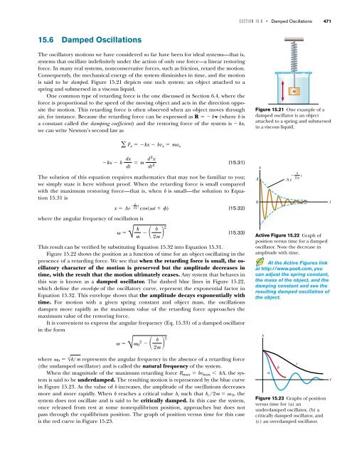
Figure 15.22 shows the position as a function of time for an object oscillating in the
presence of a retarding force. We see that when the retarding force is small, the oscillatory
character of the motion is preserved but the amplitude decreases in
time, with the result that the motion ultimately ceases. Any system that behaves in
this way is known as a damped oscillator. The dashed blue lines in Figure 15.22,
which define the envelope of the oscillatory curve, represent the exponential factor in
Equation 15.32. This envelope shows that the amplitude decays exponentially with
time. For motion with a given spring constant and object mass, the oscillations
dampen more rapidly as the maximum value of the retarding force approaches the
maximum value of the restoring force.
It is convenient to express the angular frequency (Eq. 15.33) of a damped oscillator
in the form
√ 0
2 b
2m 2
where 0 √k/m represents the angular frequency in the absence of a retarding force
(the undamped oscillator) and is called the natural frequency of the system.
When the magnitude of the maximum retarding force Rmax bvmax kA, the system
is said to be underdamped. The resulting motion is represented by the blue curve
in Figure 15.23. As the value of b increases, the amplitude of the oscillations decreases
more and more rapidly. When b reaches a critical value bc such that bc/2m 0, the
system does not oscillate and is said to be critically damped. In this case the system,
once released from rest at some nonequilibrium position, approaches but does not
pass through the equilibrium position. The graph of position versus time for this case
is the red curve in Figure 15.23.
d 2 x
dt 2
SECTION 15.6 • Damped Oscillations 471
m
Figure 15.21 One example of a
damped oscillator is an object
attached to a spring and submersed
in a viscous liquid.
A
x
b
– t
2m
Ae
0 t
Active Figure 15.22 Graph of
position versus time for a damped
oscillator. Note the decrease in
amplitude with time.
At the Active Figures link
at http://www.pse6.com, you
can adjust the spring constant,
the mass of the object, and the
damping constant and see the
resulting damped oscillation of
the object.
x
a
b
Figure 15.23 Graphs of position
versus time for (a) an
underdamped oscillator, (b) a
critically damped oscillator, and
(c) an overdamped oscillator.
c
t