Classical tidal harmonic analysis including error estimates in ...
Classical tidal harmonic analysis including error estimates in ...
Classical tidal harmonic analysis including error estimates in ...
You also want an ePaper? Increase the reach of your titles
YUMPU automatically turns print PDFs into web optimized ePapers that Google loves.
directly <strong>in</strong> matrix terms and thus relatively easy to<br />
understand and modify if required. F<strong>in</strong>ally, <strong>in</strong> order to<br />
differentiate between true determ<strong>in</strong>istic (l<strong>in</strong>e) frequencies<br />
and broad-spectrum variability, confidence <strong>in</strong>tervals for<br />
the estimated <strong>tidal</strong> parameters are computed us<strong>in</strong>g one<br />
of several user-selectable algorithms. The package is<br />
made up of a number of files each of which conta<strong>in</strong> one<br />
or more functions. User-callable functions generally<br />
have a ‘‘t ’’ prefix to prevent namespace collisions.<br />
The paper is composed of four parts. In the first the<br />
form of the equilibrium potential is described. In the<br />
second part the mathematical basis of the technique for<br />
mak<strong>in</strong>g phase/amplitude <strong>estimates</strong> is described. In the<br />
third part the generation of confidence <strong>in</strong>tervals is<br />
outl<strong>in</strong>ed. F<strong>in</strong>ally an illustrative example is discussed.<br />
2. Tidal potential<br />
The effect of gravitational force vectors from the sun<br />
and moon, F; can be written as the gradient of a scalar<br />
potential V; F ¼ rV: The magnitude of this potential<br />
at the earth’s surface at any time obviously is dependent<br />
on the relative positions of the earth, moon, and sun. In<br />
Doodson’s development (Doodson, 1954, described <strong>in</strong><br />
God<strong>in</strong>, 1972) the potential is written as a function of<br />
lunar time t (def<strong>in</strong>ed to beg<strong>in</strong> at ‘‘lunar midnight’’) and<br />
other astronomical variables (which are also functions<br />
of time):<br />
s is the mean longitude of moon, h the mean longitude<br />
of sun, p the longitude of perigee, N0 the negative of<br />
the longitude of the ascend<strong>in</strong>g node, and p0 is the<br />
longitude of perihelion, where all terms are <strong>in</strong> units of<br />
cycles. These variables can be evaluated for a given<br />
Julian date us<strong>in</strong>g the function t astron which implements<br />
formulas <strong>in</strong> Seidelmann (1992). Their effects are<br />
comb<strong>in</strong>ed with the Doodson number set for a particular<br />
constituent fi0 ; j0 ; k0 ; l0 ; m0 ; n0g <strong>in</strong>to the astronomical<br />
argument Va ¼ i0t þ j0s þ k0h þ l0p þ m0N 0 þ n0p0 : Sets<br />
with a common i0 are called a species (thus the slow,<br />
diurnal, and semidiurnal species for i0 ¼ 0; 1; and 2;<br />
respectively), and sets with common i0j0k 0 are called a<br />
subgroup. The constituent frequency s is def<strong>in</strong>ed as s ¼<br />
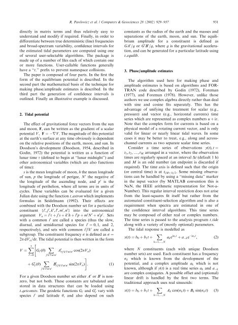
2p dVa=dt: The <strong>tidal</strong> potential is then written <strong>in</strong> the form<br />
"<br />
V ¼ X3<br />
i 0 ¼0<br />
þ G 0 i 0ðyÞ<br />
Gi 0ðyÞ<br />
X<br />
j 0 k 0 l 0 m 0 n 0<br />
X<br />
j 0 k 0 l 0 m 0 n 0<br />
A 0 i0j 0k0 l0m0 n0 cosð2pVaÞ<br />
B 0 i0j 0k0 l0m0 #<br />
n0 s<strong>in</strong>ð2pVaÞ : ð1Þ<br />
For a given Doodson number set either A 0 or B 0 is nonzero,<br />
but not both. These constants are tabulated and<br />
stored <strong>in</strong> data structures that can be loaded us<strong>in</strong>g<br />
t getconsts. The geodetic functions Gi0 and G0 i0 vary with<br />
species i0 and latitude y; and also depend on such<br />
R. Pawlowicz et al. / Computers & Geosciences 28 (2002) 929–937 931<br />
constants as the radius of the earth and the masses and<br />
separations of the earth, moon, and sun. The equilibrium<br />
amplitude for a constituent is def<strong>in</strong>ed as<br />
GA 0 =g or G 0 B 0 =g; where g is the gravitational acceleration,<br />
and can be generated for a particular latitude us<strong>in</strong>g<br />
t equilib.<br />
3. Phase/amplitude <strong>estimates</strong><br />
The algorithm used here for mak<strong>in</strong>g phase and<br />
amplitude <strong>estimates</strong> is based on algorithms and FOR-<br />
TRAN code described by God<strong>in</strong> (1972), Foreman<br />
(1977), and Foreman (1978). However, unlike those<br />
authors we use complex algebra directly rather than deal<br />
with s<strong>in</strong>e and cos<strong>in</strong>e fits separately. This has the<br />
advantage of unify<strong>in</strong>g the treatment for scalar (e.g.,<br />
pressure) and vector (e.g., horizontal currents) time<br />
series which are represented as complex numbers u þ iv:<br />
Note that the complex form for currents is based on a<br />
physical model of a rotat<strong>in</strong>g current vector, and is only<br />
valid for l<strong>in</strong>ear or nearly l<strong>in</strong>ear <strong>tidal</strong> waves. In some<br />
cases it may be better to treat, e.g., along and acrosschannel<br />
currents as two separate scalar time series.<br />
Consider a time series of observations yðtÞ; t ¼<br />
t1; t2; y; tM arranged <strong>in</strong> a vector, where the observation<br />
times are regularly spaced at an <strong>in</strong>terval Dt (default 1 h)<br />
and M is an odd number (an endpo<strong>in</strong>t is discarded if<br />
required). The time axis is def<strong>in</strong>ed such that the orig<strong>in</strong><br />
(or central time) is at tðMþ1Þ=2: Some miss<strong>in</strong>g observations<br />
can be handled by us<strong>in</strong>g a ‘‘miss<strong>in</strong>g data’’ marker<br />
<strong>in</strong> the <strong>in</strong>put vector (by MATLAB convention this is<br />
NaN, the IEEE arithmetic representation for Not-a-<br />
Number). This regular <strong>in</strong>terval restriction does not arise<br />
from the least-squares fit itself but rather from the<br />
automated constituent-selection algorithm and is also a<br />
requirement when spectra are estimated <strong>in</strong> one of<br />
the confidence <strong>in</strong>terval algorithms. This time series<br />
may be composed of either real or complex numbers.<br />
The time series is passed to the <strong>analysis</strong> program t tide<br />
along with a variety of (mostly optional) parameters.<br />
The <strong>tidal</strong> response is modelled as<br />
xðtÞ ¼b0 þ b1t þ X<br />
ake iskt<br />
þ a ke iskt<br />
; ð2Þ<br />
k¼1;y;N<br />
where N constituents (each with unique Doodson<br />
number sets) are used. Each constituent has a frequency<br />
sk which is known from the development of the<br />
potential, and a complex amplitude ak which is not<br />
known, although if yðtÞ is a real time series ak and a k<br />
are complex conjugates. A possible offset and (optional)<br />
l<strong>in</strong>ear drift is handled by the first two terms. The<br />
traditional approach uses real s<strong>in</strong>usoids:<br />
xðtÞ ¼b0 þ b1t þ X<br />
Ak cosðsktÞþBk s<strong>in</strong>ðsktÞ ð3Þ<br />
k¼1;y;N


