1 LECTURE 18: Horn Antennas (Rectangular horn antennas ...
1 LECTURE 18: Horn Antennas (Rectangular horn antennas ...
1 LECTURE 18: Horn Antennas (Rectangular horn antennas ...

Create successful ePaper yourself
Turn your PDF publications into a flip-book with our unique Google optimized e-Paper software.
<strong>LECTURE</strong> <strong>18</strong>: <strong>Horn</strong> <strong>Antennas</strong><br />
(<strong>Rectangular</strong> <strong>horn</strong> <strong>antennas</strong>. Circular apertures.) Equation Section <strong>18</strong><br />
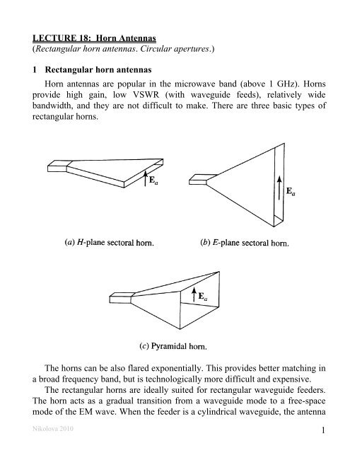
1 <strong>Rectangular</strong> <strong>horn</strong> <strong>antennas</strong><br />
<strong>Horn</strong> <strong>antennas</strong> are popular in the microwave band (above 1 GHz). <strong>Horn</strong>s<br />
provide high gain, low VSWR (with waveguide feeds), relatively wide<br />
bandwidth, and they are not difficult to make. There are three basic types of<br />
rectangular <strong>horn</strong>s.<br />
The <strong>horn</strong>s can be also flared exponentially. This provides better matching in<br />
a broad frequency band, but is technologically more difficult and expensive.<br />
The rectangular <strong>horn</strong>s are ideally suited for rectangular waveguide feeders.<br />
The <strong>horn</strong> acts as a gradual transition from a waveguide mode to a free-space<br />
mode of the EM wave. When the feeder is a cylindrical waveguide, the antenna<br />
Nikolova 2010 1
is usually a conical <strong>horn</strong>.<br />
Why is it necessary to consider the <strong>horn</strong>s separately instead of applying the<br />
theory of waveguide aperture <strong>antennas</strong> directly? It is because the so-called<br />
phase error occurs due to the difference between the lengths from the center of<br />
the feeder to the center of the <strong>horn</strong> aperture and the <strong>horn</strong> edge. This makes the<br />
uniform-phase aperture results invalid for the <strong>horn</strong> apertures.<br />
1.1 The H-plane sectoral <strong>horn</strong><br />
The geometry and the respective parameters shown in the figure below are<br />
used often in the subsequent analysis.<br />
a<br />
<br />
H<br />
lH<br />
R x<br />
R0<br />
RH<br />
2 2 A <br />
lH R0<br />
<br />
2 <br />
H<br />
Nikolova 2010 2<br />
2<br />
0 <br />
A<br />
, (<strong>18</strong>.1)<br />
A <br />
arctan 2R<br />
,<br />
(<strong>18</strong>.2)<br />
lH RHAa <br />
A <br />
z<br />
1<br />
. (<strong>18</strong>.3)<br />
4
The two fundamental dimensions for the construction of the <strong>horn</strong> are A and<br />
R H .<br />
The tangential field arriving at the input of the <strong>horn</strong> is composed of the<br />
transverse field components of the waveguide dominant mode TE10:<br />
where<br />
Zg<br />
<br />
<br />
<br />
1<br />
<br />
2a 2<br />
j 0 cos<br />
g z<br />
<br />
EyE x e<br />
a <br />
H E<br />
/ Z<br />
x y g<br />
is the wave impedance of the TE10 mode;<br />
2<br />
(<strong>18</strong>.4)<br />
<br />
g01 <br />
2a is the propagation constant of the TE10 mode.<br />
Here, 0 2 / , and is the free-space wavelength. The field that<br />
is illuminating the aperture of the <strong>horn</strong> is essentially an expanded version of the<br />
waveguide field. Note that the wave impedance of the flared waveguide (the<br />
<strong>horn</strong>) gradually approaches the intrinsic impedance of open space , as A (the<br />
H-plane width) increases.<br />
The complication in the analysis arises from the fact that the waves arriving<br />
at the <strong>horn</strong> aperture are not in phase due to the different path lengths from the<br />
<strong>horn</strong> apex. The aperture phase variation is given by<br />
e j ( R R0)<br />
. (<strong>18</strong>.5)<br />
Since the aperture is not flared in the y-direction, the phase is uniform in this<br />
direction. We first approximate the path of the wave in the <strong>horn</strong>:<br />
2 2<br />
2 2 x 1 x <br />
R R0x R0 1 R0<br />
1<br />
R<br />
<br />
0 2<br />
<br />
R<br />
. (<strong>18</strong>.6)<br />
0 <br />
The last approximation holds if x R0<br />
, or A /2<br />
R0<br />
. Then, we can assume<br />
that<br />
Nikolova 2010 3
1 x2<br />
RR0 . (<strong>18</strong>.7)<br />
2 R0<br />
Using (<strong>18</strong>.7), the field at the aperture is approximated as<br />
<br />
j x<br />
2R<br />
EaE0cos x e<br />
y <br />
A <br />
0<br />
2<br />
. (<strong>18</strong>.8)<br />
The field at the aperture plane outside the aperture is assumed equal to zero.<br />
The field expression (<strong>18</strong>.8) is substituted in the integral E I y (see Lecture 17):<br />
I E ( x, y) e dxdy ,<br />
(<strong>18</strong>.9)<br />
E<br />
y ay<br />
j( xsincosysinsin )<br />
S<br />
A<br />
A/2 <br />
b/2<br />
<br />
j x 2<br />
I E E cos x e 2R0<br />
ejxsincosdx ejy <br />
sinsindy y<br />
<br />
<br />
<br />
.<br />
(<strong>18</strong>.10)<br />
<br />
0<br />
A<br />
A/2 <br />
b/2<br />
I<br />
( , )<br />
The second integral has been already encountered. The first integral is<br />
cumbersome and the final result only is given below:<br />
where<br />
and<br />
b sin sin sin<br />
1R E<br />
0 <br />
2<br />
<br />
Iy E0 I( , ) b<br />
<br />
,<br />
(<strong>18</strong>.11)<br />
2 b<br />
sinsin <br />
2<br />
<br />
R0<br />
<br />
j sincos 2<br />
A <br />
R0<br />
<br />
j sincos 2<br />
A <br />
2<br />
2<br />
2 2 1 1<br />
<br />
I( , ) e C( s ) jS( s ) C( s ) jS( s )<br />
( 2) ( 2) ( 1) ( 1)<br />
<br />
e C t jS t C t jS t<br />
1 AR0 s1 <br />
R0u <br />
R0 2<br />
A ;<br />
1 AR0 s2 <br />
R0u <br />
R0 2<br />
A ;<br />
(<strong>18</strong>.12)<br />
Nikolova 2010 4
1 AR0 t1 <br />
R0u <br />
R0 2<br />
A ;<br />
1 AR0 t2 <br />
R0u <br />
R0 2<br />
A ;<br />
u sin cos<br />
.<br />
Cx ( ) and S( x ) are Fresnel integrals, which are defined as<br />
More accurate evaluation of E y<br />
x<br />
( ) cos 2 <br />
;<br />
2 0 <br />
( ) ( ),<br />
x<br />
( ) sin 2 <br />
;<br />
2 0 <br />
( ) ( ).<br />
Cx d C x Cx<br />
S x d S x S x<br />
(<strong>18</strong>.13)<br />
I can be obtained if the approximation in (<strong>18</strong>.6)<br />
is not made, and E a is substituted in (<strong>18</strong>.9) as<br />
y<br />
or<br />
0 <br />
Eay E<br />
xe A <br />
E e<br />
xe A <br />
The far field can be now calculated as (see Lecture 17):<br />
2 2<br />
0<br />
2 2<br />
jR0 0<br />
jR x R j R x<br />
0cos 0 cos<br />
e<br />
jr E (1 cos )sin E<br />
j Iy,<br />
4<br />
r<br />
e<br />
jr E j (1 cos )cos IE<br />
<br />
y ,<br />
4<br />
r<br />
E jE0b b sin sinsin R j r<br />
0 e<br />
1 cos <br />
<br />
<br />
2<br />
<br />
<br />
<br />
<br />
4r 2 b sinsin <br />
2<br />
<br />
I(<br />
, ) sin cos .<br />
θˆφˆ . (<strong>18</strong>.14)<br />
(<strong>18</strong>.15)<br />
(<strong>18</strong>.16)<br />
Nikolova 2010 5
The amplitude pattern of the H-plane sectoral <strong>horn</strong> is obtained as<br />
Principal-plane patterns<br />
E-plane ( 90): b sin sinsin 1 cos <br />
<br />
<br />
2<br />
<br />
E <br />
<br />
<br />
I(<br />
, )<br />
. (<strong>18</strong>.17)<br />
2 b<br />
sinsin <br />
2<br />
<br />
F<br />
E<br />
b sin sin sin<br />
1 cos <br />
<br />
<br />
2<br />
<br />
( ) <br />
<br />
<br />
<br />
2 b sinsin <br />
2<br />
<br />
(<strong>18</strong>.<strong>18</strong>)<br />
It can be shown that the second factor in (<strong>18</strong>.<strong>18</strong>) is exactly the pattern of a<br />
uniform line source of length b along the y-axis.<br />
H-plane ( 0<br />
):<br />
1cos FH( ) <br />
fH(<br />
)<br />
<br />
2 <br />
1cos I(<br />
, 0 )<br />
<br />
2 I(<br />
0 , 0 )<br />
(<strong>18</strong>.19)<br />
The H-plane pattern in terms of the I( , ) integral is an approximation, which<br />
is a consequence of the phase approximation made in (<strong>18</strong>.7). Accurate value for<br />
f ( ) is found by integrating numerically the field as given in (<strong>18</strong>.14), i.e.,<br />
H<br />
A/2<br />
x fH ( ) cos<br />
e<br />
e dx<br />
A <br />
jR22 0 xjxsin .<br />
(<strong>18</strong>.20)<br />
A/2<br />
Nikolova 2010 6
E- AND H-PLANE PATTERN OF H-PLANE SECTORAL HORN<br />
Fig. 13-12, Balanis, p. 674<br />
Nikolova 2010 7
The directivity of the H-plane sectoral <strong>horn</strong> is calculated by the general<br />
directivity expression for apertures (for derivation, see Lecture 17):<br />
D<br />
0<br />
4<br />
<br />
<br />
<br />
<br />
S<br />
2 2<br />
a<br />
S<br />
A<br />
Nikolova 2010 8<br />
2<br />
Eads<br />
A<br />
. (<strong>18</strong>.21)<br />
| E | ds<br />
The integral in the denominator is proportional to the total radiated power,<br />
b/2 A/2<br />
2<br />
2<br />
2 2<br />
rad a ds E0 xdxdy E0<br />
A<br />
S b/2 A/2<br />
<br />
Ab<br />
2 <br />
| E | cos |<br />
| . (<strong>18</strong>.22)<br />
2<br />
A<br />
In the solution of the integral in the numerator of (<strong>18</strong>.21), the field is<br />
substituted with its phase approximated as in (<strong>18</strong>.8). The final result is<br />
b 32 A<br />
4<br />
D H H<br />
H <br />
ph ( )<br />
2<br />
t<br />
ph Ab , (<strong>18</strong>.23)<br />
<br />
where<br />
t<br />
<br />
8<br />
;<br />
2<br />
2 2<br />
( 1) ( 2) ( 1) ( 2)<br />
<br />
2<br />
H<br />
ph C p C p S p S p ;<br />
64t<br />
1 1 <br />
p1 2 t<br />
<br />
1 , p2 2 t 1 8t <br />
<br />
8t<br />
;<br />
2<br />
1 A 1<br />
t .<br />
8 R0<br />
/ <br />
The factor t explicitly shows the aperture efficiency associated with the<br />
aperture cosine taper. The factor H ph is the aperture efficiency associated with<br />
the aperture phase distribution.<br />
A family of universal directivity curves is given below. From these curves,<br />
it is obvious that for a given axial length R 0 and at a given wavelength, there is<br />
an optimal aperture width A corresponding to the maximum directivity.
Stutzman<br />
It can be shown that the optimal directivity is obtained if the relation between A<br />
and R 0 is<br />
or<br />
A 3R<br />
, (<strong>18</strong>.24)<br />
Nikolova 2010 9<br />
0<br />
R 100<br />
0<br />
A R0<br />
3 . (<strong>18</strong>.25)
1.2 The E-plane sectoral <strong>horn</strong><br />
b<br />
lE<br />
E<br />
R y<br />
R0<br />
RE<br />
E-plane (y-z) cut of an E-plane<br />
sectoral <strong>horn</strong><br />
The geometry of the E-plane sectoral <strong>horn</strong> in the E-plane (y-z plane) is<br />
analogous to that of the H-plane sectoral <strong>horn</strong> in the H-plane. The analysis is<br />
following the same lines as in the previous section. The field at the aperture is<br />
approximated by [compare with (<strong>18</strong>.8)]<br />
EaE0cos x e<br />
y <br />
a <br />
Here, the approximations<br />
<br />
j y<br />
2R<br />
Nikolova 2010 10<br />
0<br />
2<br />
B<br />
z<br />
. (<strong>18</strong>.26)<br />
R R2 2<br />
0 y R0 2 2<br />
y 1 y <br />
1 R0<br />
1<br />
R<br />
<br />
0 2<br />
<br />
R<br />
<br />
0 <br />
(<strong>18</strong>.27)<br />
and<br />
1 y2<br />
RR0 2 R0<br />
are made, which are analogous to (<strong>18</strong>.6) and (<strong>18</strong>.7).<br />
(<strong>18</strong>.28)
The radiation field is obtained as<br />
2<br />
0<br />
4 j r R B<br />
a R0e <br />
j<br />
sinsin 2 2 ˆ ˆ<br />
sin cos <br />
E jE0 <br />
e<br />
4r<br />
θ φ<br />
<br />
a cos sincos (1 cos )<br />
<br />
(<strong>18</strong>.29)<br />
2<br />
<br />
Cr ( 2) jSr ( 2) Cr ( 1) jSr ( 1)<br />
.<br />
2<br />
2<br />
a <br />
1 sincos <br />
2 <br />
The arguments of the Fresnel integrals used in (<strong>18</strong>.29) are<br />
r1 <br />
<br />
R0<br />
B B<br />
<br />
R0<br />
sin sin ,<br />
2 2 <br />
r2 <br />
<br />
R0<br />
B B<br />
<br />
R0<br />
sin sin .<br />
2 2 <br />
(<strong>18</strong>.30)<br />
Principal-plane patterns<br />
The normalized H-plane pattern is found by substituting 0 in (<strong>18</strong>.29):<br />
a cos sin<br />
1 cos <br />
2<br />
H ( ) <br />
<br />
<br />
. (<strong>18</strong>.31)<br />
2<br />
2 a 1 sin<br />
2 <br />
The second factor in this expression is the pattern of a uniform-phase cosineamplitude<br />
tapered line source. (Prove!)<br />
The normalized E-plane pattern is found by substituting 90<br />
in<br />
(<strong>18</strong>.29):<br />
Cr ( 2) Cr ( 1) Sr ( 2) Sr<br />
( 1)<br />
<br />
2 2<br />
1cos 1cos E( ) fE(<br />
)<br />
<br />
2 2 4 C2( r 2<br />
0) S ( r0)<br />
<br />
. (<strong>18</strong>.32)<br />
Here, the arguments of the Fresnel integrals are calculated for 90: Nikolova 2010 11
and<br />
r1 <br />
<br />
R0<br />
B B<br />
<br />
R0<br />
sin ,<br />
2 2 <br />
r2 <br />
B B<br />
<br />
R0<br />
sin ,<br />
R0<br />
2 2 <br />
(<strong>18</strong>.33)<br />
B <br />
r0 r2( 0) . (<strong>18</strong>.34)<br />
2 R0<br />
Similar to the H-plane sectoral <strong>horn</strong>, the principal E-plane pattern can be<br />
accurately calculated if no approximation of the phase distribution is made.<br />
Then, the function fE ( ) has to be calculated by numerical integration of<br />
(compare with (<strong>18</strong>.20))<br />
B/2<br />
jR22 ( )<br />
0 y f j sin y<br />
E e e dy<br />
B<br />
/2<br />
.<br />
(<strong>18</strong>.35)<br />
Nikolova 2010 12
E- AND H-PLANE PATTERN OF E-PLANE SECTORAL HORN<br />
Fig. 13.4, Balanis, p. 660<br />
Nikolova 2010 13
Directivity<br />
The directivity of the E-plane sectoral <strong>horn</strong> is found in a manner analogous<br />
to the H-plane sectoral <strong>horn</strong>:<br />
a 32 B 4<br />
D E E<br />
E ph <br />
2<br />
tphaB,<br />
(<strong>18</strong>.36)<br />
<br />
where<br />
8<br />
t<br />
, E<br />
2 ph<br />
C2( q) S2( q) ,<br />
q2 q <br />
B<br />
2R0<br />
.<br />
A family of universal directivity curves DE parameter is given below.<br />
/ a vs. B/<br />
with R0 being a<br />
R 100<br />
Nikolova 2010 14<br />
0
The optimal relation between the flared height B and the <strong>horn</strong> length R 0 is<br />
B 2R<br />
. (<strong>18</strong>.37)<br />
1.3 The pyramidal <strong>horn</strong><br />
The pyramidal <strong>horn</strong> is probably the most popular antenna in the microwave<br />
frequency ranges (from 1 GHz up to <strong>18</strong> GHz). The feeding waveguide is<br />
flared in both directions, the E-plane and the H-plane. All results are<br />
combinations of the E-plane sectoral <strong>horn</strong> and the H-plane sectoral <strong>horn</strong><br />
analyses. The field distribution at the aperture is approximated as<br />
Nikolova 2010 15<br />
0<br />
x2 y2<br />
<br />
j 2 <br />
<br />
RE2 H2<br />
<br />
0 R <br />
0 <br />
EaE0cos x e<br />
y <br />
. (<strong>18</strong>.38)<br />
A <br />
The E-plane principal pattern of the pyramidal <strong>horn</strong> is the same as the E-plane<br />
principal pattern of the E-plane sectoral <strong>horn</strong>. The same holds for the H-plane<br />
patterns of the pyramidal <strong>horn</strong> and the H-plane sectoral <strong>horn</strong>.<br />
The directivity of the pyramidal <strong>horn</strong> can be found by introducing the phase<br />
efficiency factors of both planes and the taper efficiency factor of the H-plane:<br />
4<br />
D E H<br />
P ( )<br />
2<br />
t phph AB , (<strong>18</strong>.39)<br />
<br />
where<br />
8<br />
t<br />
;<br />
2<br />
2 2<br />
( 1) ( 2) ( 1) ( 2)<br />
<br />
2<br />
H<br />
ph C p C p S p S p ;<br />
64t<br />
1 1 <br />
p1 2 t<br />
<br />
1 , p2 2 t 1 ,<br />
8t <br />
<br />
8t<br />
<br />
<br />
E<br />
ph<br />
C2( q) S2( q) B<br />
, q<br />
2<br />
.<br />
q 2R<br />
E<br />
0<br />
2<br />
1 A 1<br />
t ;<br />
8 R / <br />
The gain of a <strong>horn</strong> is usually very close to its directivity because the radiation<br />
efficiency is very good (low losses). The directivity as calculated with (<strong>18</strong>.39)<br />
H<br />
0
is very close to measurements. The above expression is a physical optics<br />
approximation, and it does not take into account only multiple diffractions, and<br />
the diffraction at the edges of the <strong>horn</strong> arising from reflections from the <strong>horn</strong><br />
interior. These phenomena, which are unaccounted for, lead to minor<br />
fluctuations of the measured results about the prediction of (<strong>18</strong>.39). That is why<br />
<strong>horn</strong>s are often used as gain standards in antenna measurements.<br />
The optimal directivity of an E-plane <strong>horn</strong> is achieved at q 1 [see also<br />
(<strong>18</strong>.37)], E<br />
ph 0.8.<br />
The optimal directivity of an H-plane <strong>horn</strong> is achieved at<br />
t 3/8 [see also (<strong>18</strong>.24)], H<br />
ph 0.79 . Thus, the optimal <strong>horn</strong> has a phase<br />
aperture efficiency of<br />
P H E 0.632.<br />
(<strong>18</strong>.40)<br />
ph ph ph<br />
The total aperture efficiency includes the taper factor, too:<br />
P HE 0.810.632 0.51.<br />
(<strong>18</strong>.41)<br />
ph t ph ph<br />
Therefore, the best achievable directivity for a rectangular waveguide <strong>horn</strong> is<br />
about half that of a uniform rectangular aperture.<br />
We reiterate that best accuracy is achieved if H ph and E ph are calculated<br />
numerically without using the second-order phase approximations in (<strong>18</strong>.7) and<br />
(<strong>18</strong>.28).<br />
Optimum <strong>horn</strong> design<br />
Usually, the optimum (from the point of view of maximum gain) design of a<br />
<strong>horn</strong> is desired because it results in the shortest axial length. The whole design<br />
can be actually reduced to the solution of a single fourth-order equation. For a<br />
<strong>horn</strong> to be realizable, the following must be true:<br />
RE RH RP.<br />
(<strong>18</strong>.42)<br />
Nikolova 2010 16
E<br />
E<br />
R0<br />
RE<br />
y<br />
B<br />
a<br />
It can be shown that<br />
RH 0 A /2 A<br />
,<br />
RH A/2 a/2 A a<br />
(<strong>18</strong>.43)<br />
RE 0 B/2 B<br />
.<br />
REB/2 b/2 B b<br />
(<strong>18</strong>.44)<br />
The optimum-gain condition in the E-plane (<strong>18</strong>.37) is substituted in (<strong>18</strong>.44) to<br />
produce<br />
B2bB2RE 0.<br />
(<strong>18</strong>.45)<br />
There is only one physically meaningful solution to (<strong>18</strong>.45):<br />
1<br />
B b 2<br />
b2 8RE.<br />
(<strong>18</strong>.46)<br />
Similarly, the maximum-gain condition for the H-plane of (<strong>18</strong>.24) together with<br />
(<strong>18</strong>.43) yields<br />
A a 2 A ( Aa) RH A<br />
A<br />
<br />
3 <br />
.<br />
3<br />
(<strong>18</strong>.47)<br />
Since RE RH<br />
must be fulfilled, (<strong>18</strong>.47) is substituted in (<strong>18</strong>.46), which gives<br />
Nikolova 2010 17<br />
H<br />
H<br />
R0<br />
RH<br />
x<br />
A<br />
z
1 B b 2 8 A( Aa) <br />
b2<br />
.<br />
3 <br />
(<strong>18</strong>.48)<br />
Substituting in the expression for the <strong>horn</strong>’s gain<br />
4<br />
G <br />
2<br />
ap AB,<br />
<br />
(<strong>18</strong>.49)<br />
gives the relation between A, the gain G, and the aperture efficiency ap :<br />
41 G <br />
2<br />
ap A b 2 8 A( aa) <br />
b2<br />
,<br />
3 <br />
(<strong>18</strong>.50)<br />
3bG 2 3G24<br />
A4 aA3 A<br />
8 3222<br />
0.<br />
(<strong>18</strong>.51)<br />
ap ap<br />
Equation (<strong>18</strong>.51) is the optimum pyramidal <strong>horn</strong> design equation. The<br />
optimum-gain value of ap 0.51 is usually used, which makes the equation a<br />
fourth-order polynomial equation in A. Its roots can be found analytically<br />
(which is not particularly easy) and numerically. In a numerical solution, the<br />
first guess is usually set at (0) A 0.45<br />
G . Once A is found, B can be<br />
computed from (<strong>18</strong>.48) and RE RH<br />
is computed from (<strong>18</strong>.47).<br />
Sometimes, an optimal <strong>horn</strong> is desired for a given axial length R0. In this<br />
case, there is no need for nonlinear-equation solution. The design procedure<br />
follows the steps: (a) find A from (<strong>18</strong>.24), (b) find B from (<strong>18</strong>.37), and (c)<br />
calculate the gain G using (<strong>18</strong>.49) where ap 0.51.<br />
<strong>Horn</strong> <strong>antennas</strong> operate well over a bandwidth of 50 %. However, gain<br />
performance is optimal only at a given frequency. To understand better the<br />
frequency dependence of the directivity and the aperture efficiency, the plot of<br />
these curves for an X-band (8.2 GHz to 12.4 GHz) <strong>horn</strong> fed by WR90<br />
waveguide is given below ( a 0.9 in. = 2.286 cm and b 0.4 in. = 1.016 cm).<br />
Nikolova 2010 <strong>18</strong>
The gain increases with frequency, which is typical for aperture <strong>antennas</strong>.<br />
However, the curve shows saturation at higher frequencies. This is due to the<br />
decrease of the aperture efficiency, which is a result of an increased phase<br />
difference in the field distribution at the aperture.<br />
Nikolova 2010 19
The pattern of a “large” pyramidal <strong>horn</strong> ( 10.525<br />
f GHz, feeder is waveguide<br />
WR90):<br />
Nikolova 2010 20
Comparison of the E-plane patterns of a waveguide open end, “small”<br />
pyramidal <strong>horn</strong> and “large” pyramidal <strong>horn</strong>:<br />
Nikolova 2010 21
Note the multiple side lobes and the significant back lobe. They are due to<br />
diffraction at the <strong>horn</strong> edges, which are perpendicular to the E field. To reduce<br />
edge diffraction, enhancements are proposed for <strong>horn</strong> <strong>antennas</strong> such as<br />
corrugated <strong>horn</strong>s<br />
aperture-matched <strong>horn</strong>s<br />
Corrugated <strong>horn</strong>s taper the E field in the vertical direction, thus, reducing sidelobes<br />
and diffraction from edges. The overall main beam becomes smooth and<br />
nearly rotationally symmetrical (esp. for A B ). This is important when the<br />
<strong>horn</strong> is used as a feed to a reflector antenna.<br />
Nikolova 2010 22
Comparison of the H-plane patterns of a waveguide open end, “small”<br />
pyramidal <strong>horn</strong> and “large” pyramidal <strong>horn</strong>:<br />
Nikolova 2010 23
2 Circular apertures<br />
2.1 A uniform circular aperture<br />
The uniform circular aperture is approximated by a circular opening in a<br />
ground plane illuminated by a uniform plane wave normally incident from<br />
behind.<br />
E<br />
x<br />
z<br />
a<br />
The field distribution is described as<br />
Eax ˆ E0, The radiation integral is<br />
a.<br />
(<strong>18</strong>.52)<br />
I E<br />
x E0 j ˆ e ds<br />
S<br />
<br />
a<br />
Nikolova 2010 24<br />
y<br />
rr . (<strong>18</strong>.53)<br />
The integration point is at<br />
rxˆcosy ˆsin.<br />
(<strong>18</strong>.54)<br />
In (<strong>18</strong>.54), cylindrical coordinates are used, therefore,<br />
rˆr sin (coscossinsin ) sincos( )<br />
. (<strong>18</strong>.55)<br />
Hence, (<strong>18</strong>.53) becomes<br />
a 2<br />
a<br />
<br />
I E j sin cos( )<br />
x E0 e <br />
dd2 E0 J0( sin ) d<br />
0 0 <br />
0<br />
. (<strong>18</strong>.56)<br />
Here, 0<br />
J is the Bessel function of the first kind of order zero. Applying the<br />
identity
xJ0( x) dxxJ1( x)<br />
(<strong>18</strong>.57)<br />
to (<strong>18</strong>.56) leads to<br />
a<br />
IE x 2 E0 J1( asin )<br />
. (<strong>18</strong>.58)<br />
sin In this case, the equivalent magnetic current formulation of the equivalence<br />
principle is used [see Lecture 17]. The far field is obtained as<br />
ˆ e jr E θcos φˆcossin j IE<br />
x <br />
2<br />
r<br />
(<strong>18</strong>.59)<br />
j r2<br />
2 1(<br />
sin )<br />
ˆ e J a <br />
θcos φˆcossin<br />
jE0a .<br />
2r asin Principal-plane patterns<br />
E-plane ( 0):<br />
E<br />
H-plane ( 90): <br />
2 J1( asin<br />
)<br />
( ) (<strong>18</strong>.60)<br />
a sin<br />
E<br />
The 3-D amplitude pattern:<br />
<br />
2 J1( asin )<br />
( ) cos (<strong>18</strong>.61)<br />
a sin<br />
2 J 2 2 1(<br />
asin<br />
)<br />
E(<br />
, ) 1sin sin <br />
<br />
a sin<br />
Nikolova 2010 25<br />
f ( )<br />
(<strong>18</strong>.62)<br />
The larger the aperture, the less significant the cos factor is in (<strong>18</strong>.61)<br />
because the main beam in the 0 direction is very narrow and in this small<br />
solid angle cos 1.<br />
Thus, the 3-D pattern of a large circular aperture features<br />
a fairly symmetrical beam.
Example plot of the principal-plane patterns for a 3<br />
:<br />
1<br />
0.9<br />
0.8<br />
0.7<br />
0.6<br />
0.5<br />
0.4<br />
0.3<br />
0.2<br />
0.1<br />
0<br />
E-plane<br />
H-plane<br />
-15 -10 -5 0<br />
6*pi*sin(theta)<br />
5 10 15<br />
The half-power angle for the f ( ) factor is obtained at asin<br />
1.6.<br />
So,<br />
the HPBW for large apertures (a ) is given by<br />
1.6 1.6 <br />
HPBW 21/2 2arcsin 2 58.4<br />
a <br />
, deg. (<strong>18</strong>.63)<br />
a<br />
2a<br />
For example, if the diameter of the aperture is 2a 10<br />
, then HPBW 5.84.<br />
The side-lobe level of any uniform circular aperture is 0.1332 (-17.5 dB).<br />
Any uniform aperture has unity taper aperture efficiency, and its directivity<br />
can be found directly in terms of its physical area,<br />
44 D 2<br />
u A<br />
2<br />
p a . (<strong>18</strong>.64)<br />
2<br />
Nikolova 2010 26
2.2 Tapered circular apertures<br />
Many practical circular aperture <strong>antennas</strong> can be approximated as radially<br />
symmetric apertures with field amplitude distribution, which is tapered from<br />
the center toward the aperture edge. Then, the radiation integral (<strong>18</strong>.56) has a<br />
more general form:<br />
a<br />
I 2 E ( ) J ( sin ) d<br />
E<br />
x<br />
. (<strong>18</strong>.65)<br />
0<br />
0 0<br />
In (<strong>18</strong>.65), we still assume that the field has axial symmetry, i.e., it does not<br />
depend on . Often used approximation is the parabolic taper of order n:<br />
2<br />
n<br />
<br />
0<br />
Ea( )<br />
E 1 <br />
(<strong>18</strong>.66)<br />
a <br />
where E0 is a constant. This is substituted in (<strong>18</strong>.65) to calculate the respective<br />
component of the radiation integral:<br />
2<br />
n<br />
a <br />
0 0<br />
a<br />
0 <br />
I E<br />
x ( ) 2E 1 <br />
<br />
J ( sin ) d.<br />
(<strong>18</strong>.67)<br />
The following relation is used to solve (<strong>18</strong>.67):<br />
1<br />
2 n n!<br />
(1 x2) n xJ0( bx) dx J<br />
1<br />
n 1(<br />
b)<br />
bn<br />
<br />
0<br />
. (<strong>18</strong>.68)<br />
In our case, x / a and b asin . Then, I E<br />
x ( ) reduces to<br />
a2<br />
I E<br />
x ( ) E0f( ,<br />
n)<br />
, (<strong>18</strong>.69)<br />
n 1<br />
where<br />
2 n1(<br />
n1)! Jn1( asin )<br />
f( ,<br />
n)<br />
(<strong>18</strong>.70)<br />
n1<br />
asin <br />
is the normalized pattern (neglecting the angular factors such as cos and<br />
cos sin<br />
).<br />
The aperture taper efficiency is calculated to be<br />
Nikolova 2010 27
1<br />
C <br />
<br />
C <br />
n 1<br />
<br />
t<br />
<br />
<br />
. (<strong>18</strong>.71)<br />
2<br />
2 2 C(1 C) (1 C)<br />
C <br />
n1 2n1 Here, C denotes the pedestal height. The pedestal height is the edge field<br />
illumination relative to the illumination at the center.<br />
The properties of several common tapers are given in the tables below. The<br />
parabolic taper ( n 1)<br />
provides lower side lobes in comparison with the<br />
uniform distribution ( n 0)<br />
but it has a broader main beam. There is always a<br />
trade-off between low side-lobe levels and high directivity (small HPBW).<br />
More or less optimal solution is provided by the parabolic-on-pedestal aperture<br />
distribution. Moreover, this distribution approximates very closely the real case<br />
of circular reflector <strong>antennas</strong>, where the feed antenna pattern is intercepted by<br />
the reflector only out to the reflector rim.<br />
Nikolova 2010 28<br />
2
Nikolova 2010 29