A Guide to Imputing Missing Data with Stata Revision: 1.4
A Guide to Imputing Missing Data with Stata Revision: 1.4
A Guide to Imputing Missing Data with Stata Revision: 1.4

You also want an ePaper? Increase the reach of your titles
YUMPU automatically turns print PDFs into web optimized ePapers that Google loves.
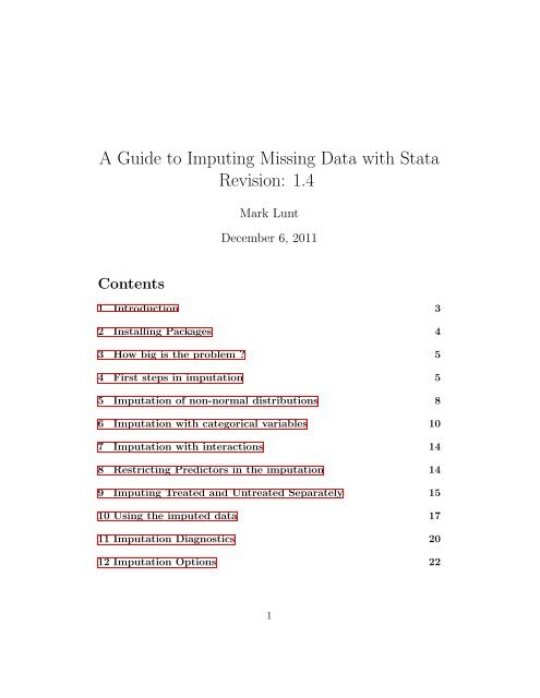
A <strong>Guide</strong> <strong>to</strong> <strong>Imputing</strong> <strong>Missing</strong> <strong>Data</strong> <strong>with</strong> <strong>Stata</strong><br />
<strong>Revision</strong>: <strong>1.4</strong><br />
Contents<br />
Mark Lunt<br />
December 6, 2011<br />
1 Introduction 3<br />
2 Installing Packages 4<br />
3 How big is the problem ? 5<br />
4 First steps in imputation 5<br />
5 Imputation of non-normal distributions 8<br />
6 Imputation <strong>with</strong> categorical variables 10<br />
7 Imputation <strong>with</strong> interactions 14<br />
8 Restricting Predic<strong>to</strong>rs in the imputation 14<br />
9 <strong>Imputing</strong> Treated and Untreated Separately 15<br />
10 Using the imputed data 17<br />
11 Imputation Diagnostics 20<br />
12 Imputation Options 22<br />
1
List of Figures<br />
1 Distribution of imputed and observed values: first attempt . . 10<br />
2 Distribution of imputed and observed values: second attempt . 12<br />
3 Distribution of imputed and observed values of DAS: common<br />
& separate imputations . . . . . . . . . . . . . . . . . . . . . . 17<br />
List of Listings<br />
1 Patterns of missing data . . . . . . . . . . . . . . . . . . . . . 6<br />
2 Regression equations used by ICE . . . . . . . . . . . . . . . . 7<br />
3 Producing his<strong>to</strong>grams of imputed data: first attempt . . . . . 9<br />
4 Producing his<strong>to</strong>grams of imputed data: second attempt . . . . 11<br />
5 <strong>Imputing</strong> from a categorical variable . . . . . . . . . . . . . . 13<br />
6 Allowing for interactions in an imputation . . . . . . . . . . . 14<br />
7 <strong>Imputing</strong> in treated and untreated separately . . . . . . . . . 16<br />
8 Subjects <strong>with</strong> complete and missing data . . . . . . . . . . . . 19<br />
9 <strong>Missing</strong> information due <strong>to</strong> missing data . . . . . . . . . . . . 21<br />
2
1 Introduction<br />
Very often in observational studies of treatment effects, we have missing data<br />
for some of the variables that we wish <strong>to</strong> balance between the treated and<br />
untreated arms of the study. This leaves us <strong>with</strong> a number of options:<br />
1. Omit the variable <strong>with</strong> the missing data from the propensity model<br />
2. Omit the individuals <strong>with</strong> the missing data from the analysis<br />
3. Reweight the individuals <strong>with</strong> complete data <strong>to</strong> more nearly approximate<br />
the distribution in all subjects<br />
4. Impute the missing data<br />
Option 1 is likely <strong>to</strong> give a biased estimate of the effect of treatment,<br />
since the treated and untreated subjects will not be balanced for the variable<br />
<strong>with</strong> missing values. Option 2 is also likely <strong>to</strong> produce a biased answer [1], as<br />
well as increasing the width of the confidence interval around the answer by<br />
reducing the number of subjects included in the analysis. Therefore, options<br />
3 and 4 are preferable: this document applies <strong>to</strong> option 4.<br />
The <strong>Stata</strong> ice routine (Imputation by Chained Equations: see [2]) is very<br />
useful for performing imputation. It can impute variables of various types<br />
(continuous, categorical, ordinal etc) using different regression methods, and<br />
uses an iterative procedure <strong>to</strong> allow for multiple missing values. For example,<br />
if you are imputing HAQ from DAS and disease duration, you may have<br />
subjects <strong>with</strong> both HAQ and DAS missing. You would then need <strong>to</strong> impute<br />
DAS, and use the imputed DAS <strong>to</strong> impute the HAQ.<br />
The imputations produced by ice take in<strong>to</strong> account the uncertainty in the<br />
predictions. That is, random noise will be added <strong>to</strong> the regression coefficients<br />
<strong>to</strong> allow for sampling error, and an error term will be added <strong>to</strong> allow for the<br />
population variation. In this way, both the mean and variance of the imputed<br />
values ought <strong>to</strong> be correct, as well as the correlations between variables.<br />
I will illustrate all of these procedures using an analysis of data from the<br />
BSRBR. We aim <strong>to</strong> perform a survival analysis of death, <strong>with</strong> the following<br />
variables regarded as confounders:<br />
3
age Age<br />
disdur Disease duration<br />
pgen Gender<br />
ovmean HAQ Score<br />
dascore Disease Activity Score<br />
dm_grp Number of previous DMARDs<br />
(Disease Modifying Anti-Rheumatic Drugs)<br />
I strongly recommend that you work through obtain the dataset that I<br />
used for this example, and work through the commands yourself (the dataset<br />
can be obtained by typing<br />
use http://personalpages.manchester.ac.uk/staff/mark.lunt/mi_example.dta<br />
in a stata command window. The best way <strong>to</strong> really understand how this<br />
works is <strong>to</strong> do it yourself. If you wish <strong>to</strong> work through this example, I suggest<br />
you start by entering the following commands:<br />
mkdir P:/mi_guide<br />
cd P:/mi_guide<br />
set more off<br />
set memory 128m<br />
log using P:/mi_guide/mi_guide.log, text replace<br />
Now you will have somewhere <strong>to</strong> s<strong>to</strong>re the results of your analysis.<br />
2 Installing Packages<br />
We are going <strong>to</strong> use four user-written add-ons <strong>to</strong> <strong>Stata</strong>, mvpatterns (<strong>to</strong> see<br />
what patterns of missing data there are), ice (<strong>to</strong> perform the imputation),<br />
mim <strong>to</strong> analyse the imputed datasets and nscore (<strong>to</strong> tranform data <strong>to</strong> and<br />
from normality) you will need <strong>to</strong> install these yourself. To install mvpatterns,<br />
type search mvpatterns, then click on dm91, and the subsequent click<br />
here <strong>to</strong> install.<br />
Unfortunately, the version of ice found by search ice is old and buggy.<br />
To get a useable version, you need <strong>to</strong> type in ssc install ice (or possibly<br />
ssc install ice, replace if you already have an old, buggy version<br />
installed). Its best <strong>to</strong> get mim from the same place, since they need <strong>to</strong> work<br />
<strong>to</strong>gether: an old version of mim may not work <strong>with</strong> a recent version of ice<br />
and vice versa. So type<br />
4
ssc install mim<br />
Finally, <strong>to</strong> install nscore type<br />
net from http://personalpages.manchester.ac.uk/staff/mark.lunt<br />
then click on the blue nscore and finally click here <strong>to</strong> install.<br />
Note that the latest version of mim will not run under stata 9.2: you must<br />
use stata 10 (which is found at M:/<strong>Stata</strong>10/wsestata.exe.<br />
3 How big is the problem ?<br />
First, we need <strong>to</strong> see how much missing data we have. We can do this <strong>with</strong><br />
the mvpatterns command:<br />
mvpatterns age disdur ovmean dascore pgen dm_grp<br />
The output of this command is shown in Listing 1.<br />
Gender data is complete, and age is almost complete. About 13% of<br />
subjects have missing HAQ scores, <strong>with</strong> substantially fewer having missing<br />
data in the other variables. Most subjects <strong>with</strong> missing data have only one<br />
or two variables missing, although a couple have 4 or 5. So that we dont<br />
change the existing data, and can tell which values are observed and which<br />
ones are imputed, we will create a new set of variables <strong>to</strong> put the imputed<br />
data in<strong>to</strong>. The commands <strong>to</strong> do this are<br />
foreach var of varlist age disdur ovmean dascore pgen dm_grp {<br />
gen ‘var’_i = ‘var’<br />
}<br />
4 First steps in imputation<br />
The next stage is <strong>to</strong> see how ice will impute these variables, using the option<br />
dryrun. The results are in Listing 2.<br />
As you can see, ice will impute each of the missing variables from all<br />
of the other 5 variables. However, it is using the regress command for all<br />
of them, which may not be appropriate. The variable dm_grp is categorical,<br />
so we should be using the commands mlogit or ologit (probably ologit<br />
in this case, since it is an ordered variable. We can use the cmd option <strong>to</strong><br />
achieve this:<br />
5
Listing 1 Patterns of missing data<br />
variables <strong>with</strong> no mv’s: pgen<br />
Variable | type obs mv variable label<br />
-------------+------------------------------------------------age<br />
| byte 13615 9<br />
disdur | byte 13485 139 Years since diagnosis<br />
ovmean | double 11854 1770 HAQ<br />
dascore | double 13220 404 DAS28<br />
dm_grp | float 13434 190<br />
---------------------------------------------------------------<br />
Patterns of missing values<br />
+------------------------+<br />
| _pattern _mv _freq |<br />
|------------------------|<br />
| +++++ 0 11390 |<br />
| ++.++ 1 1531 |<br />
| +++.+ 1 206 |<br />
| ++..+ 2 170 |<br />
| ++++. 1 129 |<br />
|------------------------|<br />
| +.+++ 1 108 |<br />
| ++.+. 2 30 |<br />
| +..++ 2 20 |<br />
| +++.. 2 12 |<br />
| ++... 3 9 |<br />
|------------------------|<br />
| .++++ 1 6 |<br />
| +..+. 3 3 |<br />
| +.... 4 3 |<br />
| +.++. 2 1 |<br />
| +.+.+ 2 1 |<br />
|------------------------|<br />
| .+.++ 2 1 |<br />
| +.+.. 3 1 |<br />
| +...+ 3 1 |<br />
| .+.+. 3 1 |<br />
| ..... 5 1 |<br />
+------------------------+<br />
6
Listing 2 Regression equations used by ICE<br />
. ice age_i disdur_i ovmean_i dascore_i pgen_i dm_grp_i, dryrun<br />
#missing |<br />
values | Freq. Percent Cum.<br />
------------+-----------------------------------<br />
0 | 11,390 83.60 83.60<br />
1 | 1,980 14.53 98.14<br />
2 | 235 1.72 99.86<br />
3 | 15 0.11 99.97<br />
4 | 3 0.02 99.99<br />
5 | 1 0.01 100.00<br />
------------+-----------------------------------<br />
Total | 13,624 100.00<br />
Variable | Command | Prediction equation<br />
------------+---------+------------------------------------------------------age_i<br />
| regress | disdur_i ovmean_i dascore_i pgen_i dm_grp_i<br />
disdur_i | regress | age_i ovmean_i dascore_i pgen_i dm_grp_i<br />
ovmean_i | regress | age_i disdur_i dascore_i pgen_i dm_grp_i<br />
dascore_i | regress | age_i disdur_i ovmean_i pgen_i dm_grp_i<br />
pgen_i | | [No missing data in estimation sample]<br />
dm_grp_i | regress | age_i disdur_i ovmean_i dascore_i pgen_i<br />
End of dry run. No imputations were done, no files were created.<br />
7
ice age_i disdur_i ovmean_i dascore_i pgen_i dm_grp_i, dryrun ///<br />
cmd(dm_grp_i: ologit)<br />
Now lets go ahead and produce some imputations. In the first instance,<br />
we will only produce a single imputation (using the option m(1)), since we<br />
want <strong>to</strong> look at the distributions of the imputed data (there are still a number<br />
of problems <strong>with</strong> our imputations that will need <strong>to</strong> be fixed before we can<br />
use them). We also need <strong>to</strong> give the name of a file in which the imputed data<br />
can be s<strong>to</strong>red. First, we will preserve our data so we can continue <strong>to</strong> work<br />
<strong>with</strong> it later. Then we do the imputation and load the imputed dataset in<strong>to</strong><br />
stata. Finally, we produce his<strong>to</strong>grams of the observed and imputed data <strong>to</strong><br />
check that the imputations are reasonable.<br />
I have added the option seed(999) <strong>to</strong> the ice command. This sets the<br />
starting value of the random number genera<strong>to</strong>r in <strong>Stata</strong>, so that the same<br />
set of random numbers will be generated if we repeat the analysis. This<br />
means that our analysis is reproducible, and that if you enter the commands<br />
in Listing 3, your output should be identical <strong>to</strong> mine.<br />
Now we can look at the imputed data, starting <strong>with</strong> continuous variables,<br />
his<strong>to</strong>grams of which are shown in Figure 1. For the HAQ score, some of the<br />
imputed values are impossible: a HAQ score lies between 0 and 3, and in fact<br />
can only take certain values in this range. <strong>Imputing</strong> data <strong>with</strong> the appropriate<br />
mean and variance leads <strong>to</strong> impossible values. A similar problem exists for<br />
disdur: values below 0 are impossible (they correspond <strong>to</strong> negative disease<br />
durations i.e. subjects who will develop their disease in the future), and yet<br />
they are imputed. The DAS has fewer problems: it is possible that out-ofrange<br />
DAS values are imputed, but it does not seem <strong>to</strong> have happened here.<br />
Only 9 values of age needed <strong>to</strong> be imputed, and they are all reasonable.<br />
5 Imputation of non-normal distributions<br />
We can get around the problem of impossible values by using the command<br />
nscore. This will transform the variables <strong>to</strong> normality, so that they can be<br />
imputed. Then invnscore can be used <strong>to</strong> convert back from the normally<br />
distributed imputed variable <strong>to</strong> the (bizarre) distributions of the original<br />
variables. The command invnscore guarantees that imputed values cannot<br />
lie outside the observed data range. The commands needed <strong>to</strong> do this given<br />
8
Listing 3 Producing his<strong>to</strong>grams of imputed data: first attempt<br />
preserve<br />
ice age_i disdur_i ovmean_i dascore_i pgen_i dm_grp_i, ///<br />
saving("mi", replace) cmd(dm_grp_i: ologit) m(1) seed(999)<br />
use mi, clear<br />
tw his<strong>to</strong>gram ovmean, width(0.125) color(gs4) || ///<br />
his<strong>to</strong>gram ovmean_i if ovmean == ., gap(50) color(gs12) ///<br />
width(0.125) legend(label(1 "Observed Values") ///<br />
label(2 "Imputed Values"))<br />
graph export haq1.eps, replace<br />
tw his<strong>to</strong>gram disdur, width(2) color(gs4) || ///<br />
his<strong>to</strong>gram disdur_i if disdur == ., gap(50) color(gs12) ///<br />
width(2) legend(label(1 "Observed Values") ///<br />
label(2 "Imputed Values"))<br />
graph export disdur1.eps, replace<br />
tw his<strong>to</strong>gram age, width(2) color(gs4) || ///<br />
his<strong>to</strong>gram age_i if age == ., gap(50) color(gs12) ///<br />
width(2) legend(label(1 "Observed Values") ///<br />
label(2 "Imputed Values"))<br />
graph export age1.eps, replace<br />
tw his<strong>to</strong>gram dascore, width(0.2) color(gs4) || ///<br />
his<strong>to</strong>gram dascore_i if dascore == ., gap(50) color(gs12) ///<br />
width(0.2) legend(label(1 "Observed Values") ///<br />
label(2 "Imputed Values"))<br />
graph export dascore1.eps, replace<br />
9
0 .2 .4 .6 .8<br />
Density<br />
0 .1 .2 .3 .4<br />
Density<br />
0 1 2 3 4<br />
Observed Values Imputed Values<br />
(a) HAQ<br />
0 2 4 6 8 10<br />
Observed Values Imputed Values<br />
(c) DAS<br />
0 .02 .04 .06<br />
Density<br />
0 .05 .1 .15 .2<br />
Density<br />
0 20 40 60 80<br />
Observed Values Imputed Values<br />
(b) Disease Duration<br />
20 40 60 80 100<br />
Observed Values Imputed Values<br />
(d) Age<br />
Figure 1: Distribution of imputed and observed values: first attempt<br />
in Listing 4 1 .<br />
It is obvious from Figure 2 that the distributions of the imputed data<br />
are much more similar <strong>to</strong> the distribution of the observed data now, and no<br />
longer follow a normal distribution.<br />
6 Imputation <strong>with</strong> categorical variables<br />
Now the imputed values all take reasonable values. However there is still one<br />
minor wrinkle: the variable dm_grp is being treated as a continuous predic<strong>to</strong>r<br />
when it is used <strong>to</strong> impute the other variables. In other words, we assume that<br />
if the HAQ is x points higher in subjects who have had 2 previous DMARDs<br />
than in those who have only had one, then it must also be x points higher<br />
1 The figures dascore3a.eps and dascore3b.eps produced by this listing will only be<br />
needed for Figure 3 later, but since the imputed data will be changed by then, I have<br />
generated them now.<br />
10
Listing 4 Producing his<strong>to</strong>grams of imputed data: second attempt<br />
res<strong>to</strong>re<br />
preserve<br />
nscore age_i disdur_i ovmean_i dascore_i, gen(nscore)<br />
ice nscore1-nscore4 pgen_i dm_grp_i, saving("mi", replace) ///<br />
cmd(dm_grp_i: ologit) m(1) seed(999)<br />
use mi, clear<br />
invnscore age_i disdur_i ovmean_i dascore_i<br />
tw his<strong>to</strong>gram ovmean, width(0.125) color(gs4) || ///<br />
his<strong>to</strong>gram ovmean_i if ovmean == ., gap(50) color(gs12) ///<br />
width(0.125) legend(label(1 "Observed Values") ///<br />
label(2 "Imputed Values"))<br />
graph export haq2.eps, replace<br />
tw his<strong>to</strong>gram disdur, width(2) color(gs4) || ///<br />
his<strong>to</strong>gram disdur_i if disdur == ., gap(50) color(gs12) ///<br />
width(2) legend(label(1 "Observed Values") ///<br />
label(2 "Imputed Values"))<br />
graph export disdur2.eps, replace<br />
tw his<strong>to</strong>gram age, width(2) color(gs4) || ///<br />
his<strong>to</strong>gram age_i if age == ., gap(50) color(gs12) ///<br />
width(2) legend(label(1 "Observed Values") ///<br />
label(2 "Imputed Values"))<br />
graph export age2.eps, replace<br />
tw his<strong>to</strong>gram dascore, width(0.2) color(gs4) || ///<br />
his<strong>to</strong>gram dascore_i if dascore == ., gap(50) color(gs12) ///<br />
width(0.2) legend(label(1 "Observed Values") ///<br />
label(2 "Imputed Values"))<br />
graph export dascore2.eps, replace<br />
tw his<strong>to</strong>gram dascore if treated == 0, width(0.2) color(gs4) || ///<br />
his<strong>to</strong>gram dascore_i if dascore == ., gap(50) color(gs12) ///<br />
width(0.2) legend(label(1 "Observed Values") ///<br />
label(2 "Imputed Values"))<br />
graph export dascore3a.eps, replace<br />
tw his<strong>to</strong>gram dascore if treated == 1, width(0.2) color(gs4) || ///<br />
his<strong>to</strong>gram dascore_i if dascore == ., gap(50) color(gs12) ///<br />
width(0.2) legend(label(1 "Observed Values") ///<br />
label(2 "Imputed Values"))<br />
graph export dascore3b.eps, replace<br />
11
0 .2 .4 .6 .8<br />
Density<br />
0 .1 .2 .3 .4<br />
Density<br />
0 1 2 3<br />
Observed Values Imputed Values<br />
(a) HAQ<br />
0 2 4 6 8 10<br />
Observed Values Imputed Values<br />
(c) DAS<br />
0 .02 .04 .06 .08<br />
Density<br />
0 .05 .1<br />
Density<br />
0 20 40 60<br />
Observed Values Imputed Values<br />
(b) Disease Duration<br />
20 40 60 80 100<br />
Observed Values Imputed Values<br />
(d) Age<br />
Figure 2: Distribution of imputed and observed values: second attempt<br />
in those who have had 6 previous DMARDs compared <strong>to</strong> those who have<br />
had only 5. This may be a reasonable assumption in some cases, but let’s<br />
suppose that it isn’t: what can we do.<br />
We can tell ice <strong>to</strong> treat dm_grp as a categorical variable when making<br />
imputations, but there are a number of steps. We need <strong>to</strong><br />
1. Create our own indica<strong>to</strong>r variables<br />
2. Tell ice not <strong>to</strong> impute these indica<strong>to</strong>rs directly, but calculate them<br />
from dm_grp<br />
3. Tell ice not <strong>to</strong> include dm_grp in its predictions, but <strong>to</strong> use our indica<strong>to</strong>rs<br />
instead.<br />
Step 1 can be performed via the command tab dm_grp, gen(dm) which<br />
will produce variables dm1, dm2, dm3, dm4, dm5, and dm6 (since dm_grp has 6<br />
levels. Although we have produced 6 variables, we will only need <strong>to</strong> include 5<br />
12
in our regression models (if you enter all 6, you will get error messages about<br />
collinearity, but still get exactly the same results).<br />
Step 2 can be achieved using the passive option: this tells ice that the<br />
variables should be calculated, not imputed, and how <strong>to</strong> calculate them. It<br />
will look like this:<br />
passive(dm1:(dm_grp==1) dm2:(dm_grp==2) dm3:(dm_grp==3) ///<br />
dm4:(dm_grp==4) dm5:(dm_grp==5))<br />
The expression in brackets for each variable tells ice how <strong>to</strong> calculate that<br />
variable, the backslash character separates each variable.<br />
Finally we need <strong>to</strong> tell ice <strong>to</strong> include dm1-dm5 in our imputations, rather<br />
than dm_grp. We can do this <strong>with</strong> the sub (for substitute) option, which will<br />
take the form sub(dm_grp: dm1-dm5). Then, in any imputation equation<br />
in which dm_grp appears, the five variables dm1-dm5 will be used instead.<br />
The full set of commands needed are shown in Listing 5.<br />
Listing 5 <strong>Imputing</strong> from a categorical variable<br />
res<strong>to</strong>re<br />
tab dm_grp, gen(dm)<br />
preserve<br />
ice age_i disdur_i ovmean_i dascore_i pgen_i dm_grp_i dm1-dm5, ///<br />
saving("mi", replace) cmd(dm_grp_i: ologit) m(1) ///<br />
passive(dm1:(dm_grp_i==1) \ dm2:(dm_grp_i==2) \ ///<br />
dm3:(dm_grp_i==3) \ dm4:(dm_grp_i==4) \ dm5:(dm_grp_i==5)) ///<br />
sub(dm_grp_i: dm1-dm5) seed(999)<br />
Note that dicho<strong>to</strong>mous variables (such as pgen) do not need this complicated<br />
treatment, provided that the two values that they take are 0 and 1.<br />
Only multicategory variables need <strong>to</strong> be treated in this way.<br />
Note also that I’ve not shown the code for converting <strong>to</strong> and from normal<br />
scores in the above example. When we impute data for real, we will have<br />
<strong>to</strong> do that, but for and example <strong>to</strong> illustrate how categorical variables work<br />
that would be an unnecessary complication.<br />
13
7 Imputation <strong>with</strong> interactions<br />
Suppose that we want <strong>to</strong> include the interaction between gender and HAQ in<br />
our imputations. Note that this would only matter if we wanted the imputation<br />
equations <strong>to</strong> include the interaction: we could calculate interactions<br />
between imputed variables in subsequent analysis as normal. However, it<br />
may be that we think that the association between DAS and HAQ differs<br />
between men and women: if we include the interaction between gender and<br />
HAQ in our imputation models, we should achieve better imputations.<br />
Including an interaction term is similar <strong>to</strong> including a categorical predic<strong>to</strong>r:<br />
we need <strong>to</strong><br />
1. Create our own variables containing the interaction terms<br />
2. Tell ice not <strong>to</strong> impute these indica<strong>to</strong>rs directly, but calculate them from<br />
pgen and ovmean<br />
We do not need <strong>to</strong> use the sub option in this case, since we do not need<br />
<strong>to</strong> remove any variables from the imputation models. The code <strong>to</strong> perform<br />
these imputations is given in Listing 6.<br />
Listing 6 Allowing for interactions in an imputation<br />
res<strong>to</strong>re<br />
gen genhaq_i = pgen_i*ovmean_i<br />
preserve<br />
ice age_i disdur_i ovmean_i dascore_i pgen_i dm_grp_i dm1-dm5 ///<br />
genhaq_i, saving("mi", replace) cmd(dm_grp_i: ologit) m(5) ///<br />
sub(dm_grp_i: dm1-dm5) passive(dm1:(dm_grp_i==1) \ ///<br />
dm2:(dm_grp_i==2) \ dm3:(dm_grp_i==3) \ dm4:(dm_grp_i==4) ///<br />
\ dm5:(dm_grp_i==5) \ genhaq: pgen_i*ovmean_i) seed(999)<br />
8 Restricting Predic<strong>to</strong>rs in the imputation<br />
So far, we have used every available predic<strong>to</strong>r <strong>to</strong> impute every possible variable.<br />
This is generally sensible: adding superfluous variables <strong>to</strong> our model<br />
14
does not have any detrimental effect on our predicted values (it can have<br />
detrimental effects on our coefficients, which is why we avoid it in general,<br />
but in this instance we are not concerned <strong>with</strong> the coefficients). However,<br />
there is an eq option that allows us <strong>to</strong> restrict the variables used in a particular<br />
imputation.<br />
For example, entering eq(ovmean_i: age_i dascore_i) would tell ice<br />
<strong>to</strong> use only the variables age_i and dascore_i when imputing ovmean.<br />
9 <strong>Imputing</strong> Treated and Untreated Separately<br />
Although the distributions of imputed values look reasonable now, there<br />
is still problem. The same imputation equation is used <strong>to</strong> impute data in<br />
treated and untreated subjects, despite the big differences in these variables<br />
between the two groups. We could simply add treatment as a predic<strong>to</strong>r <strong>to</strong><br />
all of the imputation equations, but there are still differences in the associations<br />
between (for example) DAS in the treated and untreated that are not<br />
catered for in this way. Fitting interactions between treatment and all of the<br />
predic<strong>to</strong>rs is possible, but complicated (see Section 7). Far easier would be<br />
<strong>to</strong> perform the imputations completely separately in the treated and control<br />
arms. The way <strong>to</strong> do this is illustrated in Listing 7.<br />
I have set the number of imputations <strong>to</strong> 5, since this is the dataset that<br />
will be analysed, and analysis can only be performed if there are more than 1<br />
imputation. In fact, 5 is the absolute bare minimum that would be considered<br />
acceptable: if at all possible, 10-20 should be used.<br />
Figure 3 shows the effect of imputing in the treated and untreated separately.<br />
In the <strong>to</strong>p panel, the imputation was performed in the treated and<br />
untreated as a single group. The distribution of observed DAS scores differ<br />
greatly between treated and untreated subjects, but the distribution of imputed<br />
DAS scores are similar in the treated and untreated, but unlike the<br />
observed values. In the lower panel, the imputation was performed in the<br />
treated and untreated separately. Now the distribution of imputed values in<br />
the treated and untreated subjects is similar <strong>to</strong> the observed values in that<br />
group of subjects.<br />
(Bear in mind that the distibutions of observed and imputed data do not<br />
need <strong>to</strong> be the same. For example, it may be that older subjects are less likely<br />
<strong>to</strong> complete a HAQ. Then the missing HAQs are likely <strong>to</strong> be higher than the<br />
observed HAQs. However, the associations between missingness and each of<br />
15
Listing 7 <strong>Imputing</strong> in treated and untreated separately<br />
res<strong>to</strong>re<br />
preserve<br />
keep if treated == 0<br />
nscore age_i disdur_i ovmean_i dascore_i, gen(nscore)<br />
ice nscore1-nscore4 pgen_i dm_grp_i dm1-dm5 genhaq_i, ///<br />
saving("miu", replace) cmd(dm_grp_i: ologit) m(5) ///<br />
sub(dm_grp_i: dm1-dm5) passive(dm1:(dm_grp_i==1) \ ///<br />
dm2:(dm_grp_i==2) \ dm3:(dm_grp_i==3) \ dm4:(dm_grp_i==4) \ ///<br />
dm5:(dm_grp_i==5) \ genhaq: pgen_i*nscore3) seed(999)<br />
use miu, clear<br />
invnscore age_i disdur_i ovmean_i dascore_i<br />
save, replace<br />
res<strong>to</strong>re<br />
preserve<br />
keep if treated == 1<br />
nscore age_i disdur_i ovmean_i dascore_i, gen(nscore)<br />
ice nscore1-nscore4 pgen_i dm_grp_i dm1-dm5 genhaq_i, ///<br />
saving("mit", replace) cmd(dm_grp_i: ologit) m(5) ///<br />
sub(dm_grp_i: dm1-dm5) passive(dm1:(dm_grp_i==1) \ ///<br />
dm2:(dm_grp_i==2) \ dm3:(dm_grp_i==3) \ dm4:(dm_grp_i==4) \ ///<br />
dm5:(dm_grp_i==5) \ genhaq: pgen_i*nscore3) seed(999)<br />
use mit, clear<br />
invnscore age_i disdur_i ovmean_i dascore_i<br />
append using miu<br />
tw his<strong>to</strong>gram dascore if treated == 0, width(0.2) color(gs4) || ///<br />
his<strong>to</strong>gram dascore_i if dascore == . & treated == 0, gap(50) ///<br />
color(gs12) width(0.2) ///<br />
legend(label(1 "Observed Values") ///<br />
label(2 "Imputed Values"))<br />
graph export dascore3c.eps, replace<br />
tw his<strong>to</strong>gram dascore if treated == 1, width(0.2) color(gs4) || ///<br />
his<strong>to</strong>gram dascore_i if dascore == . & treated == 1, gap(50) ///<br />
color(gs12) width(0.2) ///<br />
legend(label(1 "Observed Values") ///<br />
label(2 "Imputed Values"))<br />
graph export dascore3d.eps, replace<br />
16
0 .1 .2 .3 .4<br />
Density<br />
0 2 4 6 8 10<br />
Observed Values Imputed Values<br />
(a) Common Imputation, Untreated<br />
0 .1 .2 .3<br />
Density<br />
0 2 4 6 8 10<br />
Observed Values Imputed Values<br />
(c) Separate Imputation, Untreated<br />
0 .1 .2 .3 .4<br />
Density<br />
0 2 4 6 8 10<br />
Observed Values Imputed Values<br />
(b) Common Imputation, Treated<br />
0 .1 .2 .3 .4<br />
Density<br />
0 2 4 6 8 10<br />
Observed Values Imputed Values<br />
(d) Separate Imputation, Treated<br />
Figure 3: Distribution of imputed and observed values of DAS: common &<br />
separate imputations<br />
the variables is only minor in this instance, so the distributions of imputed<br />
and observed data should be similar.)<br />
10 Using the imputed data<br />
Having generated a set of imputations, you will want <strong>to</strong> analyse them. This<br />
is not straightforward: you need <strong>to</strong> analyse each imputed dataset separately,<br />
then combine the separate estimates in a particular way (following “Rubin’s<br />
Rules”[3]) <strong>to</strong> obtain your final estimate. Fortunately, as part of the ice package,<br />
there is a program mim which does exactly that. You simply precede<br />
whichever regression command you wanted use <strong>with</strong> mim: (provided there<br />
are at least 2 imputations, which is why we used m(5) in the ice command<br />
earlier). So, <strong>to</strong> obtain a propensity score from our imputed data, we would<br />
enter the command<br />
17
drop _merge<br />
xi: mim: logistic treated age_i disdur_i ovmean_i dascore_i ///<br />
i.pgen_i i.dm_grp_i<br />
Note that the xi command has <strong>to</strong> come before the mim command. Also,<br />
mim merges datasets as part of its analysis, so that if you have a variable<br />
called _merge in your data, mim will fail, so rename (or drop) the variable<br />
before using mim 2 .<br />
One word of warning: I have found that predict does not work as expected<br />
after mim: logistic. It seems unable <strong>to</strong> produce predicted probabilities,<br />
and outputs the linear predic<strong>to</strong>r from the logistic regression equation instead.<br />
If you wish <strong>to</strong> calculate propensity scores, you therefore need <strong>to</strong> calculate the<br />
probability yourself:<br />
predict lpi, xb<br />
gen pi = exp(lpi)/(1+exp(lpi))<br />
We can compare the effects of predicting from the complete cases and predicting<br />
from the imputed data if we also obtain the complete case propensity<br />
scores:<br />
xi: logistic treated age disdur ovmean dascore i.pgen i.dm_grp ///<br />
if _mj == 1<br />
predict pc if _mj == 1<br />
corr pc pi<br />
If you enter the above commands, you will see that for the subjects<br />
<strong>with</strong> complete data, the propensity scores are almost identical (r = 0.9964)<br />
whether we use the observed or imputed logistic regression equations. However,<br />
we can include substantially more subjects in our analysis by using the<br />
imputed data, as shown in Listing 8<br />
We have been able <strong>to</strong> include an extra 2,234 subjects in our analysis. More<br />
importantly, more than 1/3 of untreated subjects had at least one missing<br />
variable, compared <strong>to</strong> 1/8 treated subjects. Since we are short of controls <strong>to</strong><br />
begin <strong>with</strong>, the fact that we dont need <strong>to</strong> lose such a substantial number is<br />
a definite bonus.<br />
One minor point: ice creates variables called _mi and _mj, which represent<br />
the observation number and the imputation number respectively. If you<br />
2 There happened <strong>to</strong> be a _merge variable in the dataset I was working on for this<br />
example, and since I got caught out, I thought I’d mention the problem<br />
18
Listing 8 Subjects <strong>with</strong> complete and missing data<br />
. gen miss = pc == . if _mj == 1<br />
(68120 missing values generated)<br />
. tab treated miss, ro<br />
+----------------+<br />
| Key |<br />
|----------------|<br />
| frequency |<br />
| row percentage |<br />
+----------------+<br />
| miss<br />
treated | 0 1 | Total<br />
-----------+----------------------+----------<br />
0 | 1,632 959 | 2,591<br />
| 62.99 37.01 | 100.00<br />
-----------+----------------------+----------<br />
1 | 9,758 1,275 | 11,033<br />
| 88.44 11.56 | 100.00<br />
-----------+----------------------+----------<br />
Total | 11,390 2,234 | 13,624<br />
| 83.60 16.40 | 100.00<br />
19
change these variables, mim may well produce gibberish.<br />
It may be tempting <strong>to</strong> impute a single dataset, so that you dont need <strong>to</strong><br />
worry about mim. Particularly when you are exploring the data and checking<br />
for the balance of the various predic<strong>to</strong>r variables, it would be easier <strong>to</strong> use<br />
standard stata modelling commands. However, there are theoretical and<br />
empirical grounds for believing that multiple imputations can improve the<br />
precision of your parameter estimates. I would therefore recommend, having<br />
decided on your analysis strategy, <strong>to</strong> perform an entire analysis on a multiply<br />
imputed dataset.<br />
11 Imputation Diagnostics<br />
When analysing imputed data, it is vital <strong>to</strong> get some idea of how much<br />
uncertainty in your answer is due <strong>to</strong> the variation between imputations, and<br />
how much is inherent in the data itself. Ideally, you want very little variation<br />
between imputations: if your answer is consistent for multiple sets of imputed<br />
data, then it is more likely <strong>to</strong> be correct. In addition, there is always a<br />
concern that the imputations were not performed correctly: either there are<br />
associations between the variables that were not modelled, or the associations<br />
between the variables are different in those who did not respond compared <strong>to</strong><br />
those who did respond. Even if the imputed data are incorrect, the answer<br />
may still be adequate if the imputations all give similar answers.<br />
A very useful parameter <strong>to</strong> look at <strong>to</strong> answer this question is the proportion<br />
of missing information about a particular parameter, referred <strong>to</strong> as λ in<br />
[3]. Note that this parameter is not the same as the proportion of missing<br />
data: it may be that there is a lot of missing data about a weak confounder,<br />
which does not affect the parameter of interest greatly at all.<br />
Basically, the variance of the parameter you are interested is<br />
T = W + (1 + 1/m)B<br />
Where W is the mean variance of the imputations and B is the variance<br />
between imputations. So, if we had complete data, the variance would be<br />
W , so the relative increase in variance due <strong>to</strong> missing data is<br />
(1 + 1/m)B<br />
W<br />
20
There is a related number, the fraction of missing information, which has<br />
a complicated definition but generally takes similar values and assesses the<br />
same concept: how much have we lost through the missing data.<br />
Both of these parameters are produced, but not displayed, by mim. To<br />
display them, install the mfracmiss package from my homepage:<br />
1. type net from http://personalpages.manchester.ac.uk/staff/mark.lunt<br />
2. click on the blue mfracmiss<br />
3. click on click here <strong>to</strong> install.<br />
Now rerun the mim: logistic command above, then type mfracmiss,<br />
and you will get the output in Listing 9:<br />
Listing 9 <strong>Missing</strong> information due <strong>to</strong> missing data<br />
. mfracmiss<br />
--------------------------------------------------------------------<br />
Variable | Increase in Variance <strong>Missing</strong> Information<br />
-------------+-----------------------------------------------------age_i<br />
| 0.0357 0.0350<br />
disdur_i | 0.0072 0.0071<br />
ovmean_i | 0.0553 0.0537<br />
dascore_i | 0.0192 0.0190<br />
_Ipgen_i_1 | 0.0175 0.0173<br />
_Idm_grp_i_2 | 0.0090 0.0089<br />
_Idm_grp_i_3 | 0.0358 0.0351<br />
_Idm_grp_i_4 | 0.0012 0.0012<br />
_Idm_grp_i_5 | 0.0043 0.0043<br />
_Idm_grp_i_6 | 0.0124 0.0123<br />
_cons | 0.0231 0.0228<br />
--------------------------------------------------------------------<br />
There are a few surprises here. First, there was no missing data for<br />
pgen, yet there is missing information. This is due <strong>to</strong> confounding: HAQ<br />
scores are higher in the women than they are in the men, so the difference<br />
in treatment rates between men and women is partly a direct effect, and<br />
partly due <strong>to</strong> differences in HAQ. The coefficient for pgen is adjusted for<br />
differences in HAQ, but the values of HAQ (and hence the adjustment) vary<br />
21
etween imputations. Hence, the coefficent of pgen also varies. A similar<br />
argument explains the considerable effect of missing data on age, despite<br />
very few missing values for age: there is a very strong association between<br />
age and HAQ, so the missing values for HAQ affect the coefficient for age<br />
quite markedly.<br />
On the other hand, the missing information about HAQ is 5.4%, far<br />
less than the proportion of missing data. This is also because of the strong<br />
correlation between HAQ and age (and HAQ and DAS): although the data is<br />
missing, we can make a good guess as <strong>to</strong> what it should be from the values of<br />
the other variables, and therefore make good imputations. If it was unrelated<br />
<strong>to</strong> any other variable in the dataset, the proportion of missing information<br />
would be the same as the proportion of missing data.<br />
This simple example shows how important it is <strong>to</strong> look at missing information,<br />
rather than missing data. The missing information may be more than<br />
the missing data (age, pgen) or less (HAQ), depending on the exact structure<br />
of your data. Inference may be possible even if a considerable amount of<br />
data is missing, provided that there is either plenty of information about the<br />
missing data in the dataset, or that the data in question has little effect on<br />
the parameter of interest (it is a weak confounder of the variable of primary<br />
interest, for example). On the other hand, you may have complete data on<br />
the outcome and exposure of interest, yet still have missing information on<br />
relative risk, since there is missing information about confounding.<br />
12 Imputation Options<br />
Here is a recap of all of the options <strong>to</strong> ice we have used, and what they do.<br />
cmd Defines the type of regression command <strong>to</strong> be used in imputing a particular<br />
variable.<br />
m The number of imputations <strong>to</strong> perform. More iterations give greater<br />
precision, but the law of diminishing returns applies. Five is generally<br />
enough (more may be needed if there is a substantial amount of missing<br />
data), but see the discussion in [4].<br />
eq Allows the choice of variables from which <strong>to</strong> a impute a particular variable<br />
passive Identifies variables that can are functions of one or more<br />
other variables being imputed (indica<strong>to</strong>rs for a categorical variable or<br />
interaction effects).<br />
22
sub Allows the replacement of one variable by one or more other variables<br />
in the imputation models. Used <strong>to</strong> replace a categorical variable <strong>with</strong><br />
its indica<strong>to</strong>rs.<br />
seed Sets the seed for the random number genera<strong>to</strong>r, so that the same values<br />
will be imputed if the analysis is reapeated.<br />
There are a few other options <strong>to</strong> ice that may be useful:<br />
cycles If there are multiple missing variables, they all need <strong>to</strong> be imputed.<br />
The imputation equations are first calculated on the complete-case data<br />
alone, then recalculated using the observed and imputed values. As the<br />
imputed values change, the imputation equations may change, leading<br />
<strong>to</strong> further changes in the imputed values. Eventually, this process<br />
should converge. The cycles option says how many iterations of this<br />
process should be performed before producing your final imputations.<br />
The default value is 10.<br />
There are two sources of variation in the imputations: uncertainty about<br />
the coefficients in the imputation equations, and random variation in the<br />
population. Both are generally assumed <strong>to</strong> be normally distributed. If either<br />
of these assumptions are untrue, the imputed data may be unreliable.<br />
However, we have seen that we can avoid problems <strong>with</strong> a non-normal distribution<br />
in the population using nscore. There are also two options <strong>to</strong> ice<br />
<strong>to</strong> help <strong>with</strong> this problem:<br />
boot If the regression coefficients are not normally distributed, we can use<br />
the boot option <strong>to</strong> get reasonable imputations.<br />
match Rather than draw imputations from a theoretical (normal) distribution,<br />
only observed values of the variable are used. Thus the imputed<br />
values are drawn from the observed distribution. This is much slower<br />
than the default method, and the imputations may not be as reliable:<br />
see [4]. I would recommend the normal scored method outlined above<br />
in place of this option.<br />
References<br />
[1] Shafer JL, Graham JW <strong>Missing</strong> data: Our view of the state of the art<br />
Psychological Methods 2002;7:147–177.<br />
23
[2] van Buren S, Boshuizen HC, Knook DL Multiple imputation of missing<br />
blood pressure covariates in survival analysis Statistics in Medicine 1999;<br />
18:681–694.<br />
[3] Rubin DB Multiple Imputation for Nonresponse in Surveys New York: J.<br />
Wiley and Sons 1987.<br />
[4] Roys<strong>to</strong>n P Multiple imputation of missing values The <strong>Stata</strong> Journal 2004;<br />
4:227–241.<br />
24