surface mesh projection for hexahedral mesh generation by sweeping
surface mesh projection for hexahedral mesh generation by sweeping
surface mesh projection for hexahedral mesh generation by sweeping

You also want an ePaper? Increase the reach of your titles
YUMPU automatically turns print PDFs into web optimized ePapers that Google loves.
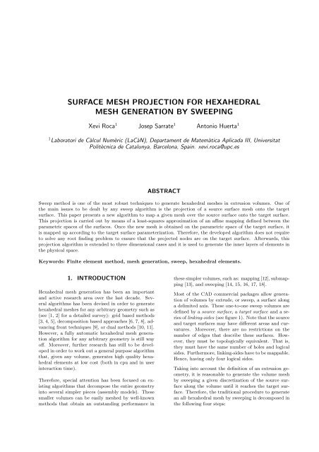
SURFACE MESH PROJECTION FOR HEXAHEDRAL<br />
MESH GENERATION BY SWEEPING<br />
Xevi Roca 1 Josep Sarrate 1 Antonio Huerta 1<br />
1 Laboratori de Càlcul Numèric (LaCàN), Departament de Matemàtica Aplicada III, Universitat<br />
Politècnica de Catalunya, Barcelona, Spain. xevi.roca@upc.es<br />
ABSTRACT<br />
Sweep method is one of the most robust techniques to generate <strong>hexahedral</strong> <strong>mesh</strong>es in extrusion volumes. One of<br />
the main issues to be dealt <strong>by</strong> any sweep algorithm is the <strong>projection</strong> of a source <strong>surface</strong> <strong>mesh</strong> onto the target<br />
<strong>surface</strong>. This paper presents a new algorithm to map a given <strong>mesh</strong> over the source <strong>surface</strong> onto the target <strong>surface</strong>.<br />
This <strong>projection</strong> is carried out <strong>by</strong> means of a least-squares approximation of an affine mapping defined between the<br />
parametric spaces of the <strong>surface</strong>s. Once the new <strong>mesh</strong> is obtained on the parametric space of the target <strong>surface</strong>, it<br />
is mapped up according to the target <strong>surface</strong> parameterization. There<strong>for</strong>e, the developed algorithm does not require<br />
to solve any root finding problem to ensure that the projected nodes are on the target <strong>surface</strong>. Afterwards, this<br />
<strong>projection</strong> algorithm is extended to three dimensional cases and it is used to generate the inner layers of elements in<br />
the physical space.<br />
Keywords: Finite element method, <strong>mesh</strong> <strong>generation</strong>, sweep, <strong>hexahedral</strong> elements.<br />
1. INTRODUCTION<br />
Hexahedral <strong>mesh</strong> <strong>generation</strong> has been an important<br />
and active research area over the last decade. Several<br />
algorithms has been devised in order to generate<br />
<strong>hexahedral</strong> <strong>mesh</strong>es <strong>for</strong> any arbitrary geometry such as<br />
(see [1, 2] <strong>for</strong> a detailed survey): grid based methods<br />
[3, 4, 5], decomposition based approaches [6, 7, 8], advancing<br />
front techniques [9], or dual methods [10, 11].<br />
However, a fully automatic <strong>hexahedral</strong> <strong>mesh</strong> <strong>generation</strong><br />
algorithm <strong>for</strong> any arbitrary geometry is still way<br />
off. Moreover, further research has still to be developed<br />
in order to work out a general purpose algorithm<br />
that, given any volume, generates high quality <strong>hexahedral</strong><br />
elements at low cost (both in cpu and in user<br />
interaction time).<br />
There<strong>for</strong>e, special attention has been focused on existing<br />
algorithms that decompose the entire geometry<br />
into several simpler pieces (assembly models). These<br />
smaller volumes can be easily <strong>mesh</strong>ed <strong>by</strong> well-known<br />
methods that obtain an outstanding per<strong>for</strong>mance in<br />
these simpler volumes, such as: mapping [12], submapping<br />
[13], and <strong>sweeping</strong> [14, 15, 16, 17, 18].<br />
Most of the CAD commercial packages allow <strong>generation</strong><br />
of volumes <strong>by</strong> extrude, or sweep, a <strong>surface</strong> along<br />
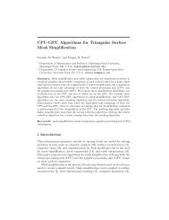
a delimited axis. These one-to-one sweep volumes are<br />
defined <strong>by</strong> a source <strong>surface</strong>, a target <strong>surface</strong> and a series<br />
of linking-sides (see figure 1). Note that the source<br />
and target <strong>surface</strong>s may have different areas and curvatures.<br />
Moreover, there are no restrictions on the<br />
number of edges that describe these <strong>surface</strong>s. However,<br />
they must be topologically equivalent. That is,<br />
they must have the same number of holes and logical<br />
sides. Furthermore, linking-sides have to be mappable.<br />
Hence, having only four logical sides.<br />
Taking into account the definition of an extrusion geometry,<br />
it is reasonable to generate the volume <strong>mesh</strong><br />
<strong>by</strong> <strong>sweeping</strong> a given discretization of the source <strong>surface</strong><br />
along the volume until it reaches the target <strong>surface</strong>.<br />
There<strong>for</strong>e, the traditional procedure to generate<br />
an all–<strong>hexahedral</strong> <strong>mesh</strong> <strong>by</strong> <strong>sweeping</strong> is decomposed in<br />
the following four steps:
source <strong>surface</strong><br />
sweep direction<br />
linking sides<br />
target <strong>surface</strong><br />
Figure 1: Example of a two and a half dimensional volume.<br />
1. Generation of a quadrilateral <strong>mesh</strong> over the<br />
source <strong>surface</strong>.<br />
2. Projection of the source <strong>mesh</strong> onto the target <strong>surface</strong><br />
(ensuring that both source and target <strong>mesh</strong><br />
have same connectivity).<br />
3. Generation of a structured quadrilateral <strong>mesh</strong><br />
over the linking-sides.<br />
4. Generation of the inner layers of nodes and elements.<br />
Note that <strong>surface</strong> <strong>mesh</strong> <strong>generation</strong> is involved in the<br />
first three steps. However, <strong>hexahedral</strong> elements are<br />
only generated in the last one. Several robust quadrilateral<br />
<strong>surface</strong> <strong>mesh</strong> <strong>generation</strong> algorithms have been<br />
developed which greatly simplify the <strong>mesh</strong>ing process<br />
involved in the first step [19, 20, 21, 22]. The gridding<br />
of the linking-sides involved in the third step can be<br />
generated using any standard structured quadrilateral<br />
<strong>surface</strong> <strong>mesh</strong> generator [2, 23]. Hence, the two main issues<br />
to be dealt <strong>by</strong> any sweep algorithm are the second<br />
and fourth step. In both steps, the <strong>mesh</strong>es to be generated<br />
(i.e. the <strong>mesh</strong> over the target <strong>surface</strong> and the<br />
inner layer <strong>mesh</strong>es) must have the same connectivity<br />
as the source <strong>surface</strong> <strong>mesh</strong>.<br />
Several algorithms have been developed to map<br />
<strong>mesh</strong>es between <strong>surface</strong>s [24]. Most of them involve<br />
an orthogonal <strong>projection</strong> of nodes onto the target <strong>surface</strong>.<br />
Note that these <strong>projection</strong>s are expensive from<br />
a computational point of view since it is necessary to<br />
solve as many root finding problems as internal points<br />
are on the grid of the source <strong>surface</strong>. In order to overcome<br />
this drawback, this paper presents a new and efficient<br />
algorithm to map a given <strong>mesh</strong> over the source<br />
<strong>surface</strong> onto the target <strong>surface</strong>. This <strong>projection</strong> is determined<br />
<strong>by</strong> means of a least-squares approximation<br />
of an affine mapping defined between the parametric<br />
representation of the loops of boundary nodes of the<br />
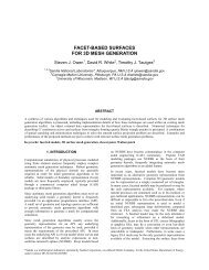
Figure 2: Available data <strong>for</strong> generating the inner layers<br />
of nodes.<br />
cap <strong>surface</strong>s. Once the new <strong>mesh</strong> is obtained on the<br />
parametric space of the target <strong>surface</strong>, it is mapped<br />
up according to the target <strong>surface</strong> parameterization.<br />
The developed algorithm to map <strong>mesh</strong>es between cap<br />
<strong>surface</strong>s can not be directly applied in order to generate<br />
the inner layer of nodes, since these layers are not<br />
defined <strong>by</strong> parametric <strong>surface</strong>s. In fact, the available<br />
data to determine the position of the inner layers of<br />
nodes is: 1.- the loops of nodes on the linking <strong>surface</strong>s,<br />
and 2.- the cap <strong>surface</strong> <strong>mesh</strong>es (see figure 2).<br />
Hence, the previous <strong>projection</strong> algorithm is extended<br />
to three dimensional space and it is used to generate<br />
the inner layers of elements in the physical space. The<br />
obtained algorithm becomes analogous to the method<br />
proposed in [14]. In order to improve the quality of the<br />
<strong>mesh</strong>es generated on each layer, the inner nodes are located<br />
using a weighted least-squares approximation of<br />
the trans<strong>for</strong>mation between the boundary nodes of the<br />
cap <strong>surface</strong>s and the boundary nodes of the layer as in<br />
[16].<br />
2. SWEEP ALGORITHM<br />
In order to ensure that the one-to-one sweep algorithm<br />
can be applied, the following requirements have to be<br />
accomplished:<br />
1. Source and target <strong>surface</strong>s must be topologically<br />
equivalent (they must have the same number of<br />
holes and logical sides).<br />
2. Linking-sides must be mappable, or equivalently,<br />
defined <strong>by</strong> four logical sides.<br />
3. Sweep volume has one source <strong>surface</strong> and one target<br />
<strong>surface</strong>.<br />
4. Sweep volume must be defined <strong>by</strong> only one axis.<br />
A detailed presentation on constraints which must be<br />
met <strong>for</strong> a volume to be sweepable, in a generic sense,<br />
are presented in [25].
Notice that the algorithm could be generalized to<br />
multi-source / multi-target geometries following the<br />
cooper tool algorithm [16, 17]. Moreover, it may also<br />
be extended to multi-axis sweep directions according<br />
to [26]. However, these objectives are beyond the<br />
scope of the present work.<br />
Sweep volumes are usually defined <strong>by</strong> commercial<br />
CAD applications. Hence, source and target <strong>surface</strong>s<br />
may be trimmed <strong>surface</strong>s (they allow a more flexible<br />
description of <strong>surface</strong>s with holes or complex boundaries).<br />
In order to properly deduce the <strong>projection</strong> algorithm<br />
between cap <strong>surface</strong>s, some details of the definition<br />
of trimmed <strong>surface</strong>s have to be revised. In particular,<br />
it is important to point out that the domain<br />
of a trimmed <strong>surface</strong>, in general, is not a rectangle<br />
[a, b] × [c, d] ⊂ R 2 in the parametric space. To be<br />
more accurate, let ϕ : V ⊂ R 2 → R 3 be the parametric<br />
definition of a <strong>surface</strong>, where V is an open and<br />
bounded set of the plane. Let DS ⊂ V be a closed<br />
subset of V . Then, a trimmed <strong>surface</strong>, S, is the image<br />
of the restriction of ϕ at the subset DS. That is,<br />
ϕ|D S : DS ⊂ V → S ⊂ R 3 , where S = ϕ(DS).<br />
From here to the end of this work we assume that a<br />
geometrical kernel is available, such that <strong>surface</strong>s are<br />
parameterized. In fact, this kernel must provide query<br />
functions <strong>for</strong> obtaining the physical coordinates of a<br />
parametric point. This requirement is necessary if the<br />
parametric space <strong>projection</strong> algorithm, presented in<br />
section 2.2, has to be implemented.<br />
2.1 Source <strong>surface</strong> <strong>mesh</strong> <strong>generation</strong><br />
In standard industrial applications, <strong>surface</strong>s are defined<br />
using any CAD software. There<strong>for</strong>e, the quadrilateral<br />
<strong>mesh</strong> generator used to discretize the source<br />
<strong>surface</strong> has to be able to work with trimmed <strong>surface</strong>s.<br />
In this paper, the source <strong>surface</strong> is discretized using an<br />
extended version to parametric <strong>surface</strong>s of a previously<br />
developed unstructured quadrilateral <strong>mesh</strong> generator<br />
[21, 22].<br />
2.2 Target <strong>surface</strong> <strong>mesh</strong> <strong>generation</strong>: the<br />
<strong>projection</strong> algorithm<br />
Once the source <strong>surface</strong>, S, is <strong>mesh</strong>ed the next step is<br />
to map it onto the target <strong>surface</strong>, T . As it has been<br />
previously noted, most of the developed algorithms to<br />
map <strong>mesh</strong>es between <strong>surface</strong>s have to solve several root<br />
finding problems. In order to overcome this drawback<br />
a new and efficient algorithm is devised to map <strong>mesh</strong>es<br />
between trimmed <strong>surface</strong>s. In fact, the mapping is<br />
defined between the parametric spaces of the <strong>surface</strong>s,<br />
DS and DT . It will be proved that determining this<br />
mapping is equivalent to finding a <strong>projection</strong> of <strong>mesh</strong>es<br />
between <strong>surface</strong>s in the physical domain. Then, the<br />
obtained <strong>mesh</strong> is mapped up according to the target<br />
<strong>surface</strong> parameterization. For some <strong>surface</strong>s, it may<br />
be necessary to smooth the new <strong>surface</strong> <strong>mesh</strong>. Note<br />
that this smoothing is also needed in other methods<br />
[24].<br />
First of all, we will show that determining a <strong>projection</strong><br />
between trimmed <strong>surface</strong>s is equivalent to finding out<br />
a <strong>projection</strong> between their parametric spaces. To this<br />
end, assume that the source and target <strong>surface</strong>s are<br />
trimmed <strong>surface</strong>s. Let<br />
ϕS : VS ⊂ R 2 → R 3<br />
ϕT : VT ⊂ R 2 → R 3<br />
be their extended parameterization, where VS and VT<br />
are two open and bounded sets of R 2 . If ϕS and ϕT<br />
are continuous and injective, the Brouwer’s theorem<br />
on invariance of domain [27] states that they are also<br />
open mappings. Since they are open mappings, their<br />
restrictions (that is, the definition of the trimmed <strong>surface</strong>s)<br />
ϕS|D S : DS ⊂ VS → S ⊂ R 3 , S := ϕS(DS)<br />
ϕT |D T : DT ⊂ VT → T ⊂ R 3 , T := ϕT (DT )<br />
are homeomorphisms in DS and DT respectively.<br />
Recall that our aim is to determine a mapping ψ :<br />
S → T such that, given a <strong>mesh</strong>, MS, over the source<br />
<strong>surface</strong>, it yields a <strong>mesh</strong>, MT , onto the target <strong>surface</strong><br />
with the same connectivities. Since S and T have the<br />
same topology it is reasonable to assume that ψ is also<br />
an homeomorphism.<br />
Since ϕS|D S , ϕT |D T and ψ are homeomorphisms, it is<br />
possible to define<br />
such that<br />
S ⊂ R 3<br />
ψ := ϕT | −1<br />
D T ◦ ψ ◦ ϕS|D S ,<br />
ψ<br />
−−−−−−→ T ⊂ R 3<br />
ϕS|DS ↑ ↑ ϕT |DT DS ⊂ R 2<br />
ψ<br />
−−−−−−→ DT ⊂ R 2<br />
(1)<br />
Under these conditions, the diagram of mappings (1)<br />
is a commutative diagram. Hence, it is feasible to find<br />
first the <strong>projection</strong> ψ, homeomorphism between the<br />
parametric domains DS and DT , and then, mapping<br />
up the new <strong>mesh</strong> onto the target <strong>surface</strong>, T , according<br />
to its parameterization, ϕT |D T , as<br />
ψ<br />
−1<br />
= ϕT |DT ◦ ψ ◦ ϕS|DS . (2)<br />
Note that it is not required to deduce the analytical<br />
−1<br />
expression of the inverse function ϕS|DS . It suffices<br />
to store the pre-images of nodal coordinates of MS <strong>by</strong><br />
ϕS|DS . This can be achieved if the application stores<br />
both the physical and the parametric coordinates of<br />
each <strong>mesh</strong> node.
n<br />
Figure 3: Boundary nodes of a non simple connected<br />
<strong>surface</strong>.<br />
There<strong>for</strong>e, special attention has to be focused on to<br />
settle the <strong>projection</strong> between DS and DT from the<br />
available data. Let n, with n ≥ 3, be the number of<br />
nodes on all the boundary loops of the cap <strong>surface</strong>s.<br />
We assume that each cap <strong>surface</strong> is delimited <strong>by</strong> one<br />
outer boundary and one inner boundary <strong>for</strong> each hole.<br />
These boundaries are previously <strong>mesh</strong>ed, and a series<br />
of loops of nodes on the boundary of the <strong>surface</strong> are<br />
obtained (see figure 3). Let US = {u i S}i=1,...,n ⊂ R 2<br />
and UT = {u i T }i=1,...,n ⊂ R 2 be the parametric coordinates<br />
of all boundary nodes of the source and target<br />
<strong>surface</strong>s, respectively. It is important to point out<br />
that the physical coordinates of these points (i.e. their<br />
images <strong>by</strong> ϕS|D S and ϕT |D T ) do not necessarily determine<br />
planar loops. The goal is to find a function ψ<br />
such that<br />
ψ(u i S) = u i T , i = 1, . . . , n. (3)<br />
Notice that it has only been required that the function<br />
ψ be a homeomorphism.<br />
n In this algorithm, the homeomorphism ψ is approximated<br />
<strong>by</strong> an affine mapping<br />
uT = ψ(uS) ≈ A(uS − u arb<br />
S ) + b, (4)<br />
where uS and uT are points on DS and DT respec-<br />
tively, A is a linear trans<strong>for</strong>mation with the origin at<br />
one arbitrary point u arb<br />
S and b is a translation vector.<br />
Un<strong>for</strong>tunately, given any two loops of boundary<br />
data, there is not an affine mapping that verifies (3).<br />
There<strong>for</strong>e, we look <strong>for</strong> a linear trans<strong>for</strong>mation, A, and<br />
a translation vector b that fits in the least-squares<br />
sense the conditions (3). Hence, A and b are such<br />
that minimizes<br />
n <br />
<br />
F (A, b) = u i <br />
T − A(u i S − u arb<br />
<br />
2<br />
S ) + b . (5)<br />
i=1<br />
It is straight<strong>for</strong>ward to show that if<br />
n<br />
u i S,<br />
u arb<br />
S := u c S = 1<br />
n<br />
i=1<br />
then<br />
b = u c T = 1<br />
n<br />
n<br />
i=1<br />
u i T . (6)<br />
There<strong>for</strong>e, the following coordinates are defined<br />
uS = uS − u c S, uT = uT − u c T , (7)<br />
such that (4) can be written as<br />
uT = ψ(uS) ≈ AuS, (8)<br />
where ψ is the expression of ψ in the new coordinates.<br />
Now the minimization problem (5) is<br />
F (A) =<br />
n <br />
<br />
u i T − Au i <br />
<br />
S<br />
2<br />
. (9)<br />
i=1<br />
Since A is a linear trans<strong>for</strong>mation, it can be written<br />
as<br />
4<br />
A = λiBi, (10)<br />
where<br />
B1 =<br />
B3 =<br />
i=1<br />
<br />
1 0<br />
, B2 =<br />
0 0<br />
<br />
0 0<br />
, B4 =<br />
1 0<br />
<br />
0 1<br />
,<br />
0 0<br />
<br />
0 0<br />
,<br />
0 1<br />
(11)<br />
is a base of the linear trans<strong>for</strong>mations from R 2 to R 2 ,<br />
and λi ∈ R, with i = 1, . . . , 4.<br />
If the scalar product of two functions<br />
is defined as<br />
< f, g > :=<br />
f : US ⊂ R 2 → R 2<br />
g : US ⊂ R 2 → R 2 ,<br />
=<br />
n<br />
< f(u i S), g(u i S) > R2 i=1<br />
n<br />
f(u i S) T · g(u i S),<br />
i=1<br />
(12)<br />
then the normal equations of the least-squares problem<br />
(9) are<br />
Nλ = d, (13)<br />
where Ni,j =< Bi, Bj >= n<br />
k=1 (Biu k S) T · Bju k S and<br />
di =< Bi, ψ >= n<br />
k=1 (Biuk S) T · u k T , with i = 1, . . . , 4<br />
and j = 1, . . . , 4.<br />
The matrix N is non-singular if and only if not all the<br />
points in US are aligned. There<strong>for</strong>e, the system (13)<br />
has a unique solution, λ 0 . From the numerical solution,<br />
λ 0 , of the linear system (13) the linear trans<strong>for</strong>mation<br />
A 0 = n i=1 λ0i Bi can be determined. There<strong>for</strong>e,<br />
using A 0 and equations (4) and (6), the following<br />
affine mapping can be established<br />
ψ 0 (uS) := A 0 (uS − u c S) + u c T<br />
(14)
In conclusion, an affine mapping (14) between parametric<br />
spaces has been found that fits, in the leastsquares<br />
sense, the loops of boundary data. This trans<strong>for</strong>mation<br />
can be used to map <strong>mesh</strong>es from DS to DT .<br />
Finally, to obtain the <strong>mesh</strong> MT it is only needed to<br />
map up the nodes onto the target <strong>surface</strong> T . To this<br />
end, an according to (2), we define<br />
ψ 0 (p) := ϕT |D T<br />
<br />
ψ 0 −1 <br />
ϕS|DS (p) <br />
, p ∈ S. (15)<br />
−1<br />
Note that, since the values of ϕS|DS are known in<br />
all nodes of MS, the new <strong>mesh</strong> on the target <strong>surface</strong><br />
can be defined as<br />
MT := ψ 0 (MS).<br />
2.3 Linking-sides <strong>mesh</strong> <strong>generation</strong><br />
Since linking-sides are always defined <strong>by</strong> four logical<br />
sides (each logical side can be composed <strong>by</strong> several<br />
edges), they can be <strong>mesh</strong>ed using any standard<br />
structured quadrilateral <strong>mesh</strong> algorithm, <strong>for</strong> instance,<br />
transfinite mapping (TFI) [2]. In order to apply the<br />
TFI method it is required that opposite logical sides<br />
will have the same number of nodes. It is important<br />
to have high quality structured <strong>mesh</strong>es on the linkingsides.<br />
Note that these <strong>mesh</strong>es determine the loops of<br />
nodes that are used later to generate the inner volume<br />
nodes in a layer <strong>by</strong> layer procedure. Thus, if these <strong>surface</strong><br />
<strong>mesh</strong>es contains folded or low quality elements,<br />
then tangled <strong>mesh</strong>es, reverse oriented or low quality<br />
<strong>hexahedral</strong> elements are obtained.<br />
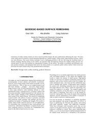
A hard test <strong>for</strong> a sweep algorithm is to <strong>mesh</strong> an extrusion<br />
volume with an S-shaped changing sweep direction,<br />
see figure 4. It is well known that obtaining<br />
a good structured <strong>mesh</strong> over an S-shaped <strong>surface</strong> is<br />
non–trivial. If nodes are generated equidistant along<br />
the edges of the S-shaped <strong>surface</strong>, then some segments<br />
of the structured <strong>surface</strong> <strong>mesh</strong> cross over each other,<br />
see figure 4(a). Thus, folded quadrilateral elements<br />
are obtained in the middle part of the <strong>surface</strong> <strong>mesh</strong>.<br />
There<strong>for</strong>e, tangled <strong>hexahedral</strong> elements are generated<br />
inside of the sweep volume.<br />
To solve this drawback, a smoothing algorithm can be<br />
used. This smoother has to be able to untangle elements<br />
and improve the <strong>mesh</strong> quality <strong>by</strong> moving inner<br />
nodes and sliding the boundary nodes along the edges.<br />
Another alternative, such that no <strong>mesh</strong> smoothing is<br />
required, is to generate nodes along S-shaped edges in<br />
such a way that the distance between opposite nodes<br />
is minimized. Hence, we have implemented an edge<br />
<strong>mesh</strong>er procedure that is able to “follow” nodes on<br />
the opposite edge of the S-shaped <strong>surface</strong>. Using this<br />
procedure, consecutive joining segments will not cross<br />
each other at the middle part of the <strong>surface</strong>, see figure<br />
4(b). The details of this edge <strong>mesh</strong>er are out of the<br />
scope of this work.<br />
(a) (b)<br />
Figure 4: S-shaped sweep volume. (a) equidistant nodes<br />
on the edges and folded elements; (b) well positioned<br />
edge nodes <strong>for</strong> the linking-sides structured <strong>mesh</strong> <strong>generation</strong>.<br />
2.4 Inner nodes and elements <strong>generation</strong><br />
Once all boundaries are <strong>mesh</strong>ed, inner nodes of the<br />
extrusion volume have to be generated. These nodes<br />
have to be placed, layer <strong>by</strong> layer, along the sweep direction.<br />
Each layer is delimited <strong>by</strong> a several loops of<br />
nodes that belongs to the structured <strong>mesh</strong>es of the<br />
linking-sides (see figure 2). In fact, <strong>for</strong> every layer<br />
there is one outer loop, and one inner loop <strong>for</strong> each<br />
hole in the sweep volume. Note that the method developed<br />
in section 2.2 can not be used here because no<br />
<strong>surface</strong> parameterization, ϕT |D T , is available <strong>for</strong> these<br />
layers. To this end, the method developed in section<br />
2.2 is extended to R 3 and a weighted least-squares approximation<br />
is developed, similar to those proposed in<br />
[14, 15, 16].<br />
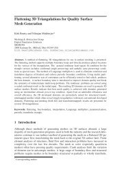
Assume that m−1 inner levels of nodes have been generated<br />
on the linking-sides along the sweep direction<br />
(see figure 5). There<strong>for</strong>e, m − 1 layers of inner nodes<br />
have to be generated. Let X0 = {x i 0}i=1,...,n ⊂ R 3 ,<br />
Xm = {x i m}i=1,...,n ⊂ R 3 and Xk = {x i k}i=1,...,n ⊂ R 3<br />
with k = 1, . . . , m − 1 be the physical coordinates of<br />
the boundary nodes of: the source <strong>surface</strong> (level 0),<br />
the target <strong>surface</strong> (level m) and the k-th level, respectively.<br />
For a given level k, with k = 1, . . . , m − 1, we<br />
look <strong>for</strong> a function φ such that<br />
x i k = φ(x i 0), i = 1, . . . , n. (16)<br />
As in section 2.2, φ is approximated <strong>by</strong> an affine mapping,<br />
concretely<br />
xk = φ(x0) ≈ A(x0 − x c 0) + x c k, (17)<br />
where x0 and xk are points on the levels 0 and k re-<br />
spectively, x c 0 = 1<br />
n<br />
n<br />
i=1 xi 0, x c k = 1<br />
n<br />
n<br />
i=1 xi k and A<br />
is a linear trans<strong>for</strong>mation with its origin at x c 0. For<br />
convenience, let<br />
x0 = x0 − x c 0, xk = xk − x c k. (18)<br />
Then, (17) can be expressed as<br />
xk = φ(x0) ≈ Ax0, (19)
Sweep direction<br />
.<br />
.<br />
level 2<br />
level 1<br />
.<br />
.<br />
.<br />
level m-1<br />
level m-2<br />
Source <strong>surface</strong> (level 0)<br />
Target <strong>surface</strong> (level m)<br />
Figure 5: Discretization of a linking side using m − 1<br />
inner levels.<br />
where φ is the expression of φ in the new coordinates<br />
(18). Similar to section 2.2, a least-squares fitting of<br />
the boundary data is per<strong>for</strong>med in order to find a linear<br />
trans<strong>for</strong>mation, that minimizes<br />
F (A) =<br />
n<br />
i=1<br />
x i k − Ax i 0 2<br />
(20)<br />
Since A is a linear trans<strong>for</strong>mation, it can be written<br />
as a linear combination of a base of the linear trans<strong>for</strong>mations<br />
from R 3 to R 3<br />
A =<br />
9<br />
λiBi, (21)<br />
i=1<br />
where λi ∈ R, with i = 1, . . . , 9, and<br />
⎛<br />
1 0<br />
⎞<br />
0<br />
⎛<br />
0 1<br />
⎞<br />
0<br />
B1 = ⎝0<br />
0 0⎠,<br />
B2 = ⎝0<br />
0 0⎠,<br />
0<br />
⎛<br />
0<br />
0<br />
0<br />
0<br />
⎞<br />
1<br />
0<br />
⎛<br />
0<br />
0<br />
0<br />
0<br />
⎞<br />
0<br />
B3 = ⎝0<br />
0 0⎠,<br />
B4 = ⎝1<br />
0 0⎠,<br />
0<br />
⎛<br />
0<br />
0<br />
0<br />
0<br />
⎞<br />
0<br />
0<br />
⎛<br />
0<br />
0<br />
0<br />
0<br />
⎞<br />
0<br />
B5 = ⎝0<br />
1 0⎠,<br />
B6 = ⎝0<br />
0 1⎠,<br />
0<br />
⎛<br />
0<br />
0<br />
0<br />
0<br />
⎞<br />
0<br />
0<br />
⎛<br />
0<br />
0<br />
0<br />
0<br />
⎞<br />
0<br />
B7 = ⎝0<br />
0 0⎠,<br />
B8 = ⎝0<br />
0 0⎠,<br />
1<br />
⎛<br />
0<br />
0<br />
0<br />
0<br />
⎞<br />
0<br />
0 1 0<br />
B9 = ⎝0<br />
0 0⎠.<br />
0 0 1<br />
(22)<br />
The normal equations of the least-squares problem<br />
(20) defined <strong>by</strong> the base (22) and the extension to<br />
R 3 of the scalar product (12) are<br />
Nλ = d, (23)<br />
where Ni,j =< Bi, Bj > and di =< Bi, φ >, with<br />
i = 1, . . . , 9 and j = 1, . . . , 9.<br />
Note that N is singular if and only if all points<br />
{x i 0}i=1,...,n are coplanar with the origin. Un<strong>for</strong>tunately,<br />
if the initial loop of points {x i 0}i=1,...,n is planar,<br />
then {x i 0}i=1,...,n are located on a plane that includes<br />
the origin. There<strong>for</strong>e, N is singular in this case.<br />
To overcome this problem, the coordinate system proposed<br />
in [14] is used<br />
x0 = x0 − (2x c 0 − x c k), xk = xk − x c 0. (24)<br />
It is known that in these new coordinates the matrix<br />
N is not singular although the boundary of the source<br />
<strong>surface</strong> is planar (except <strong>for</strong> degenerated geometries).<br />
Using these new coordinates a least-squares approximation<br />
of the boundary data can be done such that<br />
equation (20) is also minimized. That is, the normal<br />
equations (23) can also be written in the new basis<br />
(24) and the same numerical method can be used to<br />
solve the 9 × 9 linear system.<br />
Let λ 0 be the computed solution of the linear system<br />
(23). Using (24), (21), and (19), a least squares<br />
approximation of the <strong>projection</strong> between the source<br />
<strong>surface</strong> and the k-th level can be written as<br />
φ 0 k(x0) := A 0 (x0 − 2x c 0 + x c k) + x c 0<br />
(25)<br />
where A 0 is the linear trans<strong>for</strong>mation corresponding<br />
to the solution λ 0 <strong>by</strong> (21), and x0 is any point of the<br />
source <strong>surface</strong> <strong>mesh</strong>.<br />
Note that a similar process could be defined using the<br />
target <strong>surface</strong> as initial <strong>surface</strong> instead of the source<br />
<strong>surface</strong>. Hence, the nodes of the k-th level can be<br />
computed as<br />
φ m k (xm) := A m (xm − 2x c m + x c k) + x c m, (26)<br />
where xm is any point of the target <strong>surface</strong> <strong>mesh</strong>.<br />
Given two <strong>mesh</strong>es, MS and MT , over the source and<br />
target <strong>surface</strong>s, respectively, equations (25) and (26)<br />
allows to obtain two different maps of these <strong>surface</strong>s<br />
to the k-th level. There<strong>for</strong>e, and similar to [16], the<br />
following weighted trans<strong>for</strong>mation is defined<br />
φk(p) :=<br />
<br />
1 − k<br />
<br />
φ<br />
m<br />
0 k(p) + k<br />
m φm <br />
ψ 0<br />
k (p) , (27)<br />
where p ∈ MS, k = 1, . . . , m − 1, and ψ 0 is the trans<strong>for</strong>mation<br />
defined in (15). For each level, we have to<br />
compute φ 0 k and φ m k . In order to reduce the computational<br />
cost of the method, and do not recompute the<br />
set { ψ 0 (p) ∈ R 3 | p ∈ MS} <strong>for</strong> each level, the mapping<br />
relationship between nodes on MS and their images<br />
on MT can be stored once source <strong>surface</strong> <strong>mesh</strong> is projected<br />
on the target <strong>surface</strong>. In fact, it suffices to store<br />
the sequence of nodes in MT in the same order as the<br />
corresponding nodes in MS.
Thus, given a <strong>mesh</strong> MS over the source <strong>surface</strong>, the<br />
<strong>mesh</strong> Mk of the k-th level is computed as<br />
Mk := φk(MS), k = 1, . . . , m. (28)<br />
Finally, <strong>hexahedral</strong> elements are generated <strong>by</strong> joining<br />
the corresponding nodes between adjacent layers of<br />
quadrilateral <strong>mesh</strong>es.<br />
3. EXAMPLES<br />
In order to asses the quality of the sweep algorithm<br />
described above, seven examples are presented. They<br />
illustrate the capabilities of the new algorithm to <strong>mesh</strong><br />
an extrusion geometry defined <strong>by</strong> 1.- any CAD application;<br />
2.- non linear <strong>sweeping</strong> trajectories; 3.- non<br />
constant cross section along the sweep axis; 4.- non<br />
parallel cap <strong>surface</strong>s; and 5.- cap <strong>surface</strong>s with different<br />
shape and curvature. Moreover, these examples<br />
shows that the layers of inner nodes are distributed<br />
in such a way that a smooth transition between the<br />
curvatures of cap <strong>surface</strong>s is obtained. Finally, they<br />
also illustrate that the developed algorithm, coupled<br />
with volume decomposition, can be successfully used<br />
to <strong>mesh</strong> a large class of three dimensional geometries.<br />
In the first example a spring is <strong>mesh</strong>ed. The geometry<br />
is defined using a commercial CAD software. The<br />
user assigns the element size, and the application automatically<br />
determines the non linear <strong>sweeping</strong> direction.<br />
The final <strong>mesh</strong> is presented in figure 6(a). It<br />
is composed <strong>by</strong> 22740 <strong>hexahedral</strong> elements. As it can<br />
be seen, a non-structured quadrilateral <strong>mesh</strong> is generated<br />
over the cap <strong>surface</strong>s. Note that, although the<br />
<strong>sweeping</strong> axis is non linear, high quality elements are<br />
generated without a posteriori <strong>mesh</strong> smoothing.<br />
The second example presents the discretization of a<br />
bore bit with linear <strong>sweeping</strong> axis and rotated cap <strong>surface</strong>s.<br />
The <strong>mesh</strong>, see figure 6(b), is composed <strong>by</strong> 21276<br />
elements. Note that high quality elements are generated<br />
although the twisted extrusion path. Smoothing<br />
of the final <strong>hexahedral</strong> <strong>mesh</strong> was not required.<br />
In the third example, the extrusion volume is defined<br />
<strong>by</strong> two cap <strong>surface</strong>s with a different curvature. Figure<br />
6(c) shows the inner elements of the 2000 hexahedra<br />
final <strong>mesh</strong>. Note that the weighted function (27) generates<br />
layers of elements with a smooth transition of<br />
the curvature from the source <strong>surface</strong> to the target <strong>surface</strong>.<br />
Notice that no smoothing was applied to obtain<br />
this <strong>mesh</strong>.<br />
The fourth example shows the discretization of a extrusion<br />
volume defined <strong>by</strong> varying and rotating crosssections<br />
along the sweep path. These cross-sections<br />
are elliptical-shaped with different size, and just on the<br />
middle of the extrusion path becomes circular. Moreover,<br />
the cap <strong>surface</strong>s are rotated 90 degrees. The final<br />
(a)<br />
(b)<br />
(c)<br />
Figure 6: Examples of extrusion geometries <strong>mesh</strong>ed with<br />
the developed sweep algorithm. (a) spring; (b) bore bit;<br />
(c) Extrusion volume with non planar cap <strong>surface</strong>s.<br />
<strong>mesh</strong> is composed <strong>by</strong> 2373 elements, see figure 7(a). It<br />
is important to point out that to obtain the final <strong>mesh</strong><br />
no smoothing was applied on <strong>surface</strong> and inner nodes.<br />
In order to show the quality of elements inside the vol-
(a)<br />
(b) (c)<br />
Figure 7: Volume with varying elliptical cross-sections<br />
along a twisted sweep path. (a) Layer of <strong>hexahedral</strong><br />
elements at fourth-level; (b) middle layer of <strong>hexahedral</strong><br />
elements.<br />
ume, figure 7(b) shows the fourth layer of <strong>hexahedral</strong><br />
elements and figure 7(c) presents the middle layer with<br />
one circular bounding loop.<br />
The fifth example shows an application of the developed<br />
algorithm to an extrusion volume defined <strong>by</strong> two<br />
non-affine cap <strong>surface</strong>s. In this case, a smoothing algorithm<br />
had been applied on the target <strong>surface</strong> <strong>mesh</strong>.<br />
Note that in this example source <strong>surface</strong> is convex<br />
and target <strong>surface</strong> has concavities. There<strong>for</strong>e, folded<br />
quadrilateral elements appear near the concavity of<br />
the target <strong>surface</strong>. In order to unfold these quadrilateral<br />
elements it is mandatory to smooth the target<br />
<strong>surface</strong> <strong>mesh</strong>. For this example we have used the<br />
smoothing technique presented in [28]. In figure 8(a)<br />
the whole <strong>mesh</strong>, composed <strong>by</strong> 8000 <strong>hexahedral</strong> elements,<br />
is presented. Several inner layers are showed<br />
in figures 8(b), 8(c) and 8(d). Although the cap <strong>surface</strong>s<br />
ar not affine, no additional 3D global smoothing<br />
algorithm has been required in this case.<br />
The sixth example presents a sweep volume with non-<br />
(a) (b)<br />
(c) (d)<br />
Figure 8: Sweep volume with convex source face and a<br />
target face with some concavities. (a) Whole <strong>mesh</strong>; (b)<br />
layer of <strong>hexahedral</strong> elements at level six; (c) layer of <strong>hexahedral</strong><br />
elements at level eleven; (d) layer of <strong>hexahedral</strong><br />
elements at level fifteen.<br />
(a) (b)<br />
Figure 9: A <strong>sweeping</strong> volume with curved source and<br />
target <strong>surface</strong>s. (a) Top view of the final <strong>mesh</strong>; (b)<br />
Lateral view the final <strong>mesh</strong>.<br />
planar source and target <strong>surface</strong>s. Moreover, the<br />
boundary loops of these <strong>surface</strong>s, and the loops of<br />
boundary nodes <strong>for</strong> the inner layers, are non-planar<br />
too. The obtained high quality discretization is composed<br />
<strong>by</strong> 4320 elements, see figure 9. Notice that no<br />
<strong>mesh</strong> smoothing is applied to obtain the target <strong>surface</strong><br />
<strong>mesh</strong> and the final <strong>hexahedral</strong> <strong>mesh</strong>.
(a) (b)<br />
(c)<br />
Figure 10: Cube with non uni<strong>for</strong>m element size distribution.<br />
(a) Detail of the final <strong>mesh</strong> at the corner where high<br />
element concentration is prescribed; (b) View of target<br />
<strong>surface</strong> <strong>mesh</strong>; (c) Inner layer of <strong>hexahedral</strong> elements.<br />
The seventh example shows the discretization of a<br />
cube with a non–constant element size distribution.<br />
A high element concentration is prescribed at one corner<br />
of the source <strong>surface</strong>. Hence, the boundary loops<br />
of nodes are not mutually affine. Figure 10 shows the<br />
final <strong>mesh</strong> composed <strong>by</strong> 1090 elements. Two smoothing<br />
steps were required: the first one to smooth the<br />
target <strong>surface</strong> <strong>mesh</strong>, and the second one to improve<br />
the overall quality of the <strong>hexahedral</strong> <strong>mesh</strong>.<br />
The eighth example presents the application of the<br />
developed algorithm to an extrusion geometry composed<br />
<strong>by</strong> several sweep volumes. Figure 11(a) shows<br />
the discretization of a gear. The <strong>mesh</strong> is composed <strong>by</strong><br />
13712 elements. A con<strong>for</strong>mal <strong>mesh</strong> is generated over<br />
the shared <strong>surface</strong>s that compose the pieces of the volume.<br />
The last example shows the generated <strong>mesh</strong> <strong>for</strong> a crank<br />
shaft model, see figure 11(b). It is composed <strong>by</strong> 15800<br />
elements. As in the previous example, a con<strong>for</strong>mal<br />
<strong>mesh</strong> is obtained <strong>for</strong> this multi-block geometry.<br />
(a)<br />
(b)<br />
Figure 11: Examples of extrusion geometries <strong>mesh</strong>ed<br />
with the developed sweep algorithm. (a) gear; (b) crank<br />
shaft.<br />
4. CONCLUSIONS<br />
In this paper a new algorithm to project <strong>mesh</strong>es between<br />
two topologically equivalent <strong>surface</strong>s has been<br />
presented. It has been successfully implemented in a<br />
sweep tool to <strong>mesh</strong> extrusion geometries. This <strong>projection</strong><br />
is determined <strong>by</strong> means of a least-squares approximation<br />
of a trans<strong>for</strong>mation defined between the<br />
loops of boundary nodes of the cap <strong>surface</strong>s in the<br />
parametric spaces. Once the new <strong>mesh</strong> is obtained in<br />
the parametric space, it is mapped up according the<br />
target <strong>surface</strong> parameterization. This <strong>projection</strong> algorithm<br />
has been extended to three dimensional spaces.<br />
Then, it has been used to generate the inner nodes
<strong>for</strong> a sweep tool. In this case, the inner nodes are<br />
located using a weighted least-squares approximation<br />
of the trans<strong>for</strong>mation between the boundary nodes of<br />
the cap <strong>surface</strong>s and the boundary nodes of the layer.<br />
Finally, several examples have been presented to show<br />
the new algorithm capabilities.<br />
References<br />
[1] Tautges T.J. “The <strong>generation</strong> of <strong>hexahedral</strong><br />
<strong>mesh</strong>es <strong>for</strong> assembly geometry: survey and<br />
progress.” International Journal <strong>for</strong> Numerical<br />
Methods in Engineering, vol. 50, no. 12, 2617–<br />
2642, 2001<br />
[2] Thompson J.F., Warsi Z.U.A., Mastin C.W. Numerical<br />
grid <strong>generation</strong>: foundations and applications.<br />
Elsevier North-Holland, 1985<br />
[3] Schneiders R. “A grid-based algorithm <strong>for</strong> the<br />
<strong>generation</strong> of <strong>hexahedral</strong> element <strong>mesh</strong>es.” Engineering<br />
with Computers, vol. 12, no. 3-4, 168–177,<br />
1996<br />
[4] Taghavi R. “Automatic, parallel and fault tolerant<br />
<strong>mesh</strong> <strong>generation</strong> from CAD.” Engineering<br />
with Computers, vol. 12, no. 3-4, 178–185, 1996<br />
[5] Dhondt G. “A new automatic <strong>hexahedral</strong> <strong>mesh</strong>er<br />
based on cutting.” International Journal <strong>for</strong> Numerical<br />
Methods in Engineering, vol. 50, no. 9,<br />
2109–2126, 2001<br />
[6] Price M.A., Armstrong C.G., Sabin M.A. “Hexahedral<br />
Mesh Generation <strong>by</strong> Medial Surface Subdivision:<br />
Part I. Solids with Convex Edges.” International<br />
Journal <strong>for</strong> Numerical Methods in Engineering,<br />
vol. 38, no. 19, 3335–3359, 1995<br />
[7] Price M.A., Armstrong C.G. “Hexahedral <strong>mesh</strong><br />
<strong>generation</strong> <strong>by</strong> medial <strong>surface</strong> subdivision: Part II.<br />
Solids with flat and concave edges.” International<br />
Journal <strong>for</strong> Numerical Methods in Engineering,<br />
vol. 40, no. 1, 111–136, 1997<br />
[8] Taghavi R. “Automatic block decomposition<br />
of parametrically changing volumes.” Oil &<br />
Gas Science and Technology-Revue De L Institut<br />
Francais Du Petrole, vol. 54, no. 2, 193–196,<br />
1999<br />
[9] Blacker T.D., Meyers R.J. “Seams and Wedges in<br />
Plastering - a 3-D Hexahedral Mesh Generation<br />
Algorithm.” Engineering with Computers, vol. 9,<br />
no. 2, 83–93, 1993<br />
[10] Tautges T.J., Blacker T., Mitchell S.A. “The<br />
whisker weaving algorithm: A connectivity-based<br />
method <strong>for</strong> constructing all-<strong>hexahedral</strong> finite element<br />
<strong>mesh</strong>es.” International Journal <strong>for</strong> Numerical<br />
Methods in Engineering, vol. 39, no. 19,<br />
3327–3349, 1996<br />
[11] Calvo N.A., Idelsohn S.R. “All-<strong>hexahedral</strong> element<br />
<strong>mesh</strong>ing: Generation of the dual <strong>mesh</strong> <strong>by</strong><br />
recurrent subdivision.” Computer Methods in Applied<br />
Mechanics and Engineering, vol. 182, no. 3-<br />
4, 371–378, 2000<br />
[12] Cook W.A., Oakes W.R. “Mapping methods <strong>for</strong><br />
generating three-dimensional <strong>mesh</strong>es.” Computers<br />
In Mechanical Engineering, pp. 67–72, 1982<br />
[13] White D. Automatic, quadrilateral and <strong>hexahedral</strong><br />
<strong>mesh</strong>ing of pseudo-cartesian geometries using<br />
virtual subdivision. Master in science, Brigham<br />
Young University, 1996<br />
[14] Knupp P.M. “Next-Generation Sweep Tool: A<br />
Method For Generating All-Hex Meshes On Two-<br />
And-One-Half Dimensional Geomtries.” 7th International<br />
Meshing Roundtable, pp. 505–513.<br />
Sandia National Lab, 1998<br />
[15] Knupp P.M. “Applications of <strong>mesh</strong> smoothing:<br />
Copy, morph, and sweep on unstructured quadrilateral<br />
<strong>mesh</strong>es.” International Journal <strong>for</strong> Numerical<br />
Methods in Engineering, vol. 45, no. 1,<br />
37–45, 1999<br />
[16] Blacker T. “The Cooper Tool.” 5th International<br />
Meshing Roundtable, pp. 13–30. Sandia National<br />
Laboratories, 1996<br />
[17] Lai M., Benzley S., White D. “Automated <strong>hexahedral</strong><br />
<strong>mesh</strong> <strong>generation</strong> <strong>by</strong> generalized multiple<br />
source to multiple target <strong>sweeping</strong>.” International<br />
Journal <strong>for</strong> Numerical Methods in Engineering,<br />
vol. 49, no. 1-2, 261–275, 2000<br />
[18] Staten M.L., Canann S.A., Owen S.J. “BM-<br />
Sweep: Locating interior nodes during <strong>sweeping</strong>.”<br />
Engineering with Computers, vol. 15, no. 3, 212–<br />
218, 1999<br />
[19] Blacker T.D., Stephenson M.B. “Paving - a<br />
New Approach to Automated Quadrilateral Mesh<br />
Generation.” International Journal <strong>for</strong> Numerical<br />
Methods in Engineering, vol. 32, no. 4, 811–<br />
847, 1991<br />
[20] Cass R.J., Benzley S.E., Meyers R.J., Blacker<br />
T.D. “Generalized 3-D paving: An automated<br />
quadrilateral <strong>surface</strong> <strong>mesh</strong> <strong>generation</strong> algorithm.”<br />
International Journal <strong>for</strong> Numerical Methods in<br />
Engineering, vol. 39, no. 9, 1475–1489, 1996
[21] Sarrate J., Huerta A. “Efficient unstructured<br />
quadrilateral <strong>mesh</strong> <strong>generation</strong>.” International<br />
Journal <strong>for</strong> Numerical Methods in Engineering,<br />
vol. 49, no. 10, 1327–1350, 2000<br />
[22] Sarrate J., Huerta A. “Automatic <strong>mesh</strong> <strong>generation</strong><br />
of nonstructured quaadrilateral <strong>mesh</strong>es over<br />
curved <strong>surface</strong>s in R 3 .” European Congress on<br />
Computational Methods in Applied Sciences and<br />
Engineering, ECCOMAS. Barcelona, Spain, 2000<br />
[23] Haber R., Shephard M.S., Abel J.F., Gallagher<br />
R.H., Greenberg D.P. “A General Two-<br />
Dimensional, Graphical Finite-Element Preprocessor<br />
Utilizing Discrete Transfinite Mappings.”<br />
International Journal <strong>for</strong> Numerical Methods in<br />
Engineering, vol. 17, no. 7, 1015–1044, 1981<br />
[24] Goodrich D. Generation of all-quadrilateral <strong>surface</strong><br />
<strong>mesh</strong>ers <strong>by</strong> <strong>mesh</strong> morphing. Master in science,<br />
Brigham Young University, 1997<br />
[25] White D.R., Tautges T.J. “Automatic scheme<br />
selection <strong>for</strong> toolkit hex <strong>mesh</strong>ing.” International<br />
Journal <strong>for</strong> Numerical Methods in Engineering,<br />
vol. 49, no. 1-2, 127–144, 2000<br />
[26] Miyoshi K., Blacker T. “Hexahedral Mesh Generation<br />
Using Multi-Axis Cooper Algorithm.”<br />
9th International Meshing Roundtable, pp. 89–97.<br />
Sandia National Laboratories, Albuquerque, New<br />
Mexico, 2000<br />
[27] Hatcher A. Algebraic topology. Cambridge University<br />
Press, New York, 2002<br />
[28] Sarrate J., Huerta A. “A new approach to minimize<br />
the distortion of quadrilateral and <strong>hexahedral</strong><br />
<strong>mesh</strong>es.” 4th European congress on computational<br />
methods in applied sciences and engineering.<br />
Jyväskylä, Finland, 2004