Receding Front Method: a New Approach Applied to Generate ...

A-PDF Split DEMO : Purchase from www.A-PDF.com to remove the watermark 

Receding Front Method: a New Approach Applied to 

Generate Hexahedral Meshes of Outer Domains 

Xevi Roca, Eloi Ruiz-Gironés, and Josep Sarrate 

Laboratori de Càlcul Numèric (LaCàN), 

Departament de Matemàtica Aplicada III, 

Universitat Politècnica de Catalunya, 

Jordi Girona 1-3, E–08034 Barcelona, Spain 

{xevi.roca,eloi.ruiz,jose.sarrate}@upc.edu ⋆⋆ 

Summary. Two of the most successful methods to generate unstructured hexahedral meshes 

are the grid-based methods and the advancing front methods. On the one hand, the grid-based 

methods generate high quality elements in the inner part of the domain using an inside-outside 

approach. On the other hand, advancing front methods generate high quality hexahedra near 

the boundary using an outside-inside approach. In this paper we propose the receding front 

method, an original approach that combines the advantages of both methodologies: we use 

an inside-outside mesh generation approach by means of a reversed front advance. We apply 

this approach to mesh outer domains. To reproduce the shape of the boundaries, we first precompute 

the mesh fronts by combining two solutions of the Eikonal equation on a tetrahedral 

reference mesh. Then, to generate high quality elements, we expand the quadrilateral surface 

mesh of the inner body towards the unmeshed external boundary using the pre-computed 

fronts as a guide. Further research is under way in order to apply the proposed method to more 

complicated geometries. 

Key words: Mesh generation, unstructured hexahedra, eikonal equation 

1 Introduction 

During the last two decades several general-purpose algorithms for fully automatic 

hexahedral mesh generation have been proposed, see [1, 2, 3, 4, 5, 6] for a survey. 

However, none of the existent algorithms is robust, automatic and generates highquality 

meshes for any initial geometry. There are two families of methods that almost 

fulfill all these requirements, the grid-based and the advancing front methods. 

In fact, these approaches are the most successful methodologies to obtain a generalpurpose 

hex-meshing algorithm. Furthermore, the grid-based and advancing front 

⋆⋆ This work was partially sponsored by the Spanish Ministerio de Ciencia e Innovación under 

grants DPI2007-62395, BIA2007-66965 and CGL2008-06003-C03-02/CLI and by Universitat 

Politècnica de Catalunya (UPC)

2 X. Roca, E. Ruiz-Gironés and J. Sarrate 

methods have advantages and disadvantages that complement each other. Thus, we 

can consider how to obtain a hexahedral meshing approach that presents only the 

advantages, and avoids the disadvantages, of these two methods. 

On the one hand, the grid-based methods [7, 8, 9, 10] are the only family of 

robust and fully automatic hexahedral mesh generation algorithms. In addition, they 

generate high-quality meshes in the inner part of the mesh. These advantages are 

possible because the mesh is generated from inside-to-outside. However, the gridbased 

methods generate low quality hexahedra near the boundary and the final mesh 

depends on the spatial orientation of the domain. These drawbacks appear because 

the inner mesh does not have layers of hexahedra that progressively adapt to the 

boundary shape of the domain. 

On the other hand, the advancing front methods [11, 12, 13] generate high-quality 

meshes near the boundary (boundary sensitive) that do not depend on the orientation 

of the object (orientation insensitive), see details on hex-meshing requirements in 

[2]. This is possible because the elements are generated layer by layer following the 

shape of the boundary surface. However, the advancing front methods are less robust 

and automatic. When the fronts are advanced, from the boundary to the inner 

part, they collide and can delimit complex voids. Specifically, if the advancing front 

method starts with a prescribed quadrilateral mesh of the boundary (constrained approach) 

[11] the resulting void is, in general terms, over-constrained and cannot be 

meshed. On the contrary, the versions of the advancing front method that start without 

a prescribed mesh of the boundary (unconstrained approach) [12, 13] can always 

generate a hexahedral mesh for the void. To this end, usually the unconstrained methods 

[12, 13, 14, 15] use a tetrahedral mesh to generate a hexahedral one. However, 

the quality of the mesh of the inner void is not guaranteed because it results from 

splitting each tetrahedron in four hexahedra. These disadvantages at the inner part 

are caused because the elements are generated from outside-to-inside. Note that also 

there are constrained methods that directly transform a tetrahedral mesh into a hexdominant 

mesh [16, 17]. 

Summarizing, by generating elements from inside-to-outside we can avoid the 

front collisions that lead to unmeshed voids or low-quality inner meshes. Moreover, 

by generating the elements using fronts (layers of elements) we can obtain meshes 

that reproduce properly the shape of the domain boundary. In this work we apply 

these advantages to mesh outer domains. To this end, we propose: 

• To generate layers of elements from inside-to-outside. Hence, we present the first 

receding front method. That is, a reversed advancing front method. 

• To pre-compute the fronts (or layers of hexahedra) combining two solutions of 

the Eikonal equation. One solution determines the distance to the inner part and 

the other the distance to the outer boundary. The level sets of the combination of 

both solutions determine the fronts. 

This work is clearly related to the grid-based and advancing front methods. However, 

the grid-based methods do not generate layers of hexahedra from inside-tooutside 

that smoothly adapt to the boundary of the domain. In addition, the advancing 

front methods do not start to generate layers of hexahedra from inside the domain. In

Receding Front Method: Applied to Outer Domains 3 

this sense, the proposed approach is different to both methodologies. Furthermore, 

we propose to pre-compute the fronts by solving the Eikonal equation. It is important 

to point out that there are other mesh generation works that use the Eikonal equation. 

In his seminar work, Sethian proposes a method to advance structured meshes by 

solving the Eikonal equation [18]. Another front propagation method based on the 

Eikonal equation is presented in [19]. In [20, 21], the authors show how to obtain 

the medial axis transform (MAT) by means of the Eikonal equation. Nevertheless, 

this is the first work were two solutions of the Eikonal equation are combined to 

pre-compute the fronts and obtain an unstructured hexahedral mesh. 

The remainder of the paper is organized as follows. First, we present a 2D motivation 

example in Section 2. According to this motivation, in Section 3 we detail 

the receding front method. Specifically, we present how to pre-compute the fronts, 

generate the meshes between the fronts and refine the resulting hexahedral fronts. 

Finally, in Section 4 we present several example meshes that demonstrate the capabilities 

of the first implementation of the receding front method. 

2 2D Motivation 

To illustrate and clarify the basis of the receding front method in 3D, we consider a 

2D example. Specifically, we present a smooth domain with a three-branched skeleton 

to be meshed with quadrilateral (hexahedral) elements. With the help of this 

domain we first review the main advantages and disadvantages of the grid-based 

and advancing front methods. Then, we outline the proposed receding front method 

which combines the advantages of both methods. 

Given a domain, the grid-based methods first generate a quadrilateral (hexahedral) 

mesh in the inner part of the domain, Fig. 1(a). Then, the remaining void between 

the inner mesh and the boundary, Fig. 1(b), has to be meshed. To this end, 

several new nodes are created on the boundary. These nodes are connected with the 

quadrilateral elements of the boundary of the inner mesh to form the last layer of 

hexahedra, Fig. 1(c). Since the boundary of the inner mesh is not adapted to the 

shape of the domain boundary, the last layer of hexahedra can present low quality 

elements. We would like to remark that this approach is robust and can be applied to 

general geometries to obtain meshes with high-quality elements in the inner part. 

The advancing front methods generate layers of elements (fronts) that start at the 

domain boundary and layer by layer reach (advance towards) the inner part of the 

domain. At the last step, several elements that connect the fronts close the remaining 

void. There are two families of advancing front methods: the constrained [11] and 

the unconstrained approaches [12, 13]. 

The constrained approach generates a first layer of elements, Fig. 2(a), that 

matches with a prescribed mesh of the boundary. Then, several layers of elements 

are generated by merging and matching the elements that are in front of the last 

layer, Fig. 2(b). Since the process starts with a prescribed mesh of the boundary 

and advance inwards, the last voids in the inner part of the domain can be complex


(a) (b) (c) 

Fig. 1. Several steps of a grid-based method: (a) inner mesh; (b) void between boundary and 

inner mesh; and (c) final mesh. 

(a) (b) (c) 

Fig. 2. Several steps of a constrained advancing front method: (a) first front; (b) last front and 

contours of the previous fronts; and (c) unmeshed void. 

(a) (b) (c) 

Fig. 3. Several steps of an unconstrained advancing front method: (a) fronts and final void; (b) 

simplicial mesh of the void; and (c) splitting simplicial mesh. 

and over-constrained. Specifically, in the 3D case the advance can lead to remaining 

voids that cannot be meshed, Fig. 2(c). 

The unconstrained approach relaxes the hex-meshing problem by considering 

that the domain boundary is not meshed. The meshing process starts at the boundary 

and provides a decomposition of the domain in several layers, Fig. 3(a). The process 

stops when the inner void can be discretized with a hex-meshing primitive. Since the 

inner void results from successive offsets of the boundary, it can be as much difficult 

to hex-mesh as the initial domain. Thus, there are configurations where the inner 

void can not be meshed with a high-quality hex-meshing primitive. However, it is 

always possible to generate a hexahedral mesh. To this end, this approach generates 

a simplicial mesh of the unrecognized inner void, Fig. 3(b). The simplicial mesh can 

always be split in quadrilateral (hexahedral) elements, Fig. 3(c). Then, the boundary 

of this inner mesh is propagated through the layers to the boundary of the domain.


(a) (b) 

(c) (d) 

Fig. 4. Pre-computing the fronts: (a) outer boundary and inner seed; (b) level sets from inside 

to outside; (c) level sets from outside to inside; and (d) combining inside-to-outside with 

outside-to-inside level sets. 

The quality of the inner elements is not guaranteed because they are originated by 

a simplicial mesh. Moreover, the boundary of the inner mesh is propagated through 

the domain to the boundary. Thus, the inner mesh determines the structure and the 

quality of the inner part of the boundary curves (surfaces). It is important to point out 

that the element quality close to the boundary features is ensured because it is a front 

approach, except when the boundary has a very sharp dihedral angle. In addition, 

this approach is fully automatic and provides high-quality meshes for a wide range 

of geometries. 

To combine the advantages of both the grid-based and the advancing front methods, 

herein we propose the receding front method. To apply this methodology we 

require an initial mesh (seed) of the inner part of the domain, Fig. 4(a). Note that for 

the specific case of meshing the outer domain of a given body the initial mesh is a 

quadrilateral mesh of the body surface. This way, we can decouple the problem of 

generating the inner seed from the front generation process. The fronts that determine 

the layers of elements can be pre-computed. Specifically, we generate an offset of the 

shape of the inner seed towards the boundary, Fig. 4(b), and an offset of the boundary 

shape inwards, Fig. 4(c). These offsets are obtained as the level sets of two solutions 

of the Eikonal equation, Section 3.1. One solution is related to the boundary of the 

inner part and the other one to the outer boundary. To compute these solutions we 

use an edge-based solver on a triangular (tetrahedral) mesh [22]. Then, we combine 

both solutions to obtain a function of the domain that reproduces the inner shape in 

the inner part and the boundary close to the outer part, Fig. 4(d). Then, the fronts are 

obtained as the level sets of this function. Finally, these fronts can be used as a guide 

to generate layers of elements starting from the inner seed and finishing in the outer 

boundary, Fig. 5. To this end, we need to consider a set of templates that determine 

how to offset the previous layer of elements to the new front, Section 3.2. Moreover,


(a) (b) 

(c) (d) 

Fig. 5. Layers of elements for the receding front method: (a) first layer; (b) second layer; (c) 

third layer; and (d) final layer. 

we have to consider a set of refinement rules that ensure that the element size is not 

surpassed. The resulting procedure generates layers of elements that progressively 

morph from the shape of the inner seed to the shape of the outer boundary. Moreover, 

starting from the inner part we can avoid over-constrained or complex inner 

voids. 

3 The Receding Front Method 

The receding front method is decomposed into two steps. First, we pre-compute a set 

of fronts between the inner and the outer boundaries. Second, we expand the quadrilateral 

mesh of the inner boundary towards the unmeshed outer boundary according 

to the pre-computed fronts. 

3.1 Pre-computing the Fronts 

Given a domain Ω ⊂ Rn , the Eikonal equation is the following non-linear partial 

differential equation 

∇d = f in Ω 

d| U⊂{Ω∪∂Ω} = 0, 

(1) 

where f is a known function and · is the euclidean norm. To solve the Eikonal 

equation, we first generate a tetrahedral mesh of the domain. Then, we obtain the 

solution for that discretization by means of an edge-based solver [22]. 

For f = 1 the solution d is the distance from ∂Ω. For f = 1 

h(x) the level sets of 

the solution d follow the size field h(x) defined for each x ∈ ∂Ω. In this work we 

consider f = 1.

@ Win 

(a) 

@ Wout 


@ Win 

(b) 

@ Wout 

Fig. 6. Solution of the Eikonal equation starting from: (a) the outer boundary (∂Ωout) and, (b) 

the inner boundary (∂Ωin). 

In our applications we consider a domain bounded by an inner object (which 

defines the inner boundary of the domain, ∂Ωin) and a smooth outer boundary denoted 

by ∂Ωout. In order to find a distance field that takes into account the distance 

from each inner point to both boundaries we first consider the following problem, 

see Figure 6(a): 

∇dout = 1 in Ω 

(2) 

dout|∂Ωout = 0, 

where dout 0. The solution of this problem provides the distance to the outer 

boundary. Then, we consider the problem, see Figure 6(b): 

 

∇din = 1 in Ω 

din|∂Ωin = 0, 

(3) 

where din 0. The solution of this problem provides the distance to the inner boundary. 

Note that we use the same tetrahedral mesh to solve Equations (2) and (3). The 

combined distance field, u, is defined as: 

u := 

dout 

dout + din 

. (4) 

Note that the combined distance field verifies 0 u 1, and at the boundaries 

of the domain it also verifes that u|∂Ωout = 0 and u|∂Ωin = 1. Moreover, the contours 

of u close ∂Ωout are similar to dout whereas the contours of u close ∂Ωin are similar 

to din. That is, the combined distance field reproduces the shapes of the inner and 

outer boundaries close to them. 

Finally, we extract m level sets of the combined distance field u. These level 

sets determine the fronts used to advance the mesh from the meshed inner boundary 

towards the meshed outer boundary. Algorithm 1 details the proposed procedure to 

generate the level sets of the distance field.


Algorithm 1: Generate level sets ordered from inside to outside 

1 

2 

3 

4 

Input: ∂Ωin, inner boundary; ∂Ωout, outer boundary; m, number of level sets 

Output: L, level sets ordered from inside to outside 

Scalar field din ← solve Eikonal equation in Ω starting at ∂Ωin 

Scalar field dout ← solve Eikonal equation in Ω starting at ∂Ωout 

Scalar field u ← dout 

dout+d in 

Level sets L ← extract m iso-surfaces of u from 1 to 0 

Algorithm 2: Generate hexahedra between level sets 

1 

2 

3 

4 

5 

6 

7 

8 

Input: L, ordered level sets; Q0, quad surface mesh of the inner object 

Output: H, final hexahedral mesh 

Hex-mesh H ← {∅} 

foreach level set ℓ in L do 

Quad-mesh Qℓ ← get the quadrilateral mesh on ℓ 

detect geometric features of Qℓ 

Level set ℓnext ← get next level set to ℓ 

Hex-mesh Hℓ ← offset Qℓ from ℓ to ℓnext 

H ← H ∪ Hℓ 

refine H according to the prescribed element size 

3.2 Meshing the Fronts 

From a quadrilateral surface mesh of the inner boundary we want to generate an 

unstructured hexahedral mesh of the domain without prescribing a quadrilateral surface 

mesh of the outer boundary. To this end, we detail in Algorithm 2 the proposed 

procedure. Each level-set will delimit a layer of hexahedral elements. Therefore, we 

have to describe the procedure to expand a quadrilateral mesh on level set ℓ to level 

set ℓ + 1. We first detect the geometric features of Qℓ and classify the edges of the 

quad mesh as corner, reversal and end according to the angles defined by the adjacent 

faces, φ. An edge is classified as corner if π/4 ≤ φ < 3π/4; as reversal if 

3π/4 ≤ φ < 5π/4; and as end if 5π/4 ≤ φ < 7π/4. Otherwise the edge is not 

a feature and it is classified as side. Once the edges are classified, we proceed to 

classify the nodes of the quadrilateral mesh. A node is classified as feature node if 

it belongs to three o more feature edges. Otherwise, the node is classified as nonfeature 

node. Note that these two classifications will determine the topology of the 

hexahedral mesh for the considered level. 

Once the edges and the nodes of the quadrilateral surface mesh are classified, 

we expand the quadrilateral mesh to the next level set. The expansion process is 

performed taking into account the topological entities of the quadrilateral mesh. First, 

we consider the faces of the quadrilateral mesh. Figure 7 illustrates the expansion of 

a quadrilateral face. Second, we expand the feature edges of the quadrilateral mesh


Fig. 7. Face template. 

corner reversal 

end 

Fig. 8. Edge templates. 

3C 2C - 1E 1C - 2E 3E 

3C - 3E 2C - 2E 2R - 1C 2R - 1E 

Fig. 9. Vertex templates. 

according to their classification. Figure 8 illustrates the templates used to expand 

feature edges of the quadrilateral mesh. Third, we expand the feature nodes of the 

quadrilateral mesh according to the classification of adjacent feature edges. Figure 9 

illustrates the templates used to expand feature nodes of the quadrilateral mesh. 

The size of the new hexahedra may differ from the prescribed element size. For 

this reason, a local refinement process is performed at each level. The edges of the 

new boundary that are longer than the prescribed element size are marked to be refined. 

Then, each hexahedron is replaced by a given template of hexahedra depending 

on the marked edges to be refined. To this end, we use the method proposed in [23]


where the templates introduced by [9, 10] are adapted to marked edges. At this point, 

the algorithm of front meshing is iterated until all the fronts are discretized. 

4 Examples 

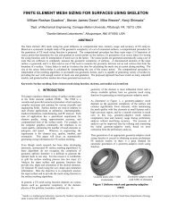
In this section we present four meshes of the outer domain of a given object created 

with the receding front method. In all the cases the starting seed is a quadrilateral 

mesh of the inner surface. The user input is the element size of the quadrilateral 

mesh and the number of levels of the mesh. 

4.1 Long box 

The first example presents a mesh generated on the exterior domain of a long box. 

The box is located inside a smooth domain. Note that the inner boundary only contains 

feature edges classified as corner, see Section 3.1. Figure 10(a) presents the 

tetrahedral mesh used to compute the solution of both Eikonal equations. Figure 

10(b) presents the pre-computed fronts as detailed in Section 3.1. Note that we have 

prescribed four levels in order to generate the mesh. Figure 10(c) shows a general 

view of the hexahedral mesh while Figure 10(d) illustrates a longitudinal cut of the 

mesh. Although the quadrilateral surface mesh of the inner box is structured, the final 

mesh contains unstructured nodes both in the interior and on the boundary of the 

mesh. For instance, in Figure 10(c) we highlight a node with three adjacent hexahedra 

and in Figure 10(d) we mark an inner node with six adjacent hexahedra. 

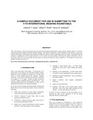
4.2 Pentagonal star 

The second example presents the generated mesh for the domain delimited by a star 

placed inside a sphere. In this case the definition of the domain contains feature 

edges classified as corner and end. The final mesh is composed by eight levels of 

hexahedral elements. Figure 11(b) shows a cut of the mesh and Figure 11(c) presents 

a detail of the unstructured mesh. Note that the expansion of the seed surface mesh 

generates unstructured elements in order to reach properly the outer boundary. 

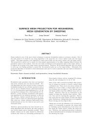
4.3 Smooth Object with a Reversal Feature 

The objective of the third example is to show that using a refinement procedure we 

can respect the prescribed element size in the final mesh. To this end, we discretize 

a domain delimited by a flat object inside an ellipsoid. This geometry only contains 

feature edges classified as reversal. First, we generate a hexahedral mesh without 

using the local refinement process described in Section 3.1. Figure 12 shows the final 

mesh. Note that the obtained element size near the outer boundary is greater than the 

obtained element size near the inner boundary. In order to preserve the prescribed 

element size, in each level we perform a local refinement. Figure 13 illustrates that 

the final mesh reproduces with more fidelity the prescribed element size. Note that 

in both cases an unstructured mesh is obtained.


(a) (b) 

(c) (d) 

Fig. 10. Hexahedral mesh for the exterior domain of the long box. (a) Tetrahedral mesh used 

to solve the Eikonal equation. (b) Level sets of the combined distance field. (c) General view 

of the hexahedral mesh. (d) Longitudinal cut of the hexahedral mesh. 

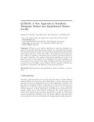
4.4 Space Capsule 

One of the advantages of the proposed approach is that it is straightforward to stretch 

the elements in the normal direction of the fronts. To this end, we use a blending 

function [24] that modifies the combined distance field u introduced in equation (4): 

u = eαu−1 

eα , (5) 

− 1 

where α ∈ R. If α < 0, the levels are concentrated towards the outer boundary. 

If α > 0, the levels are concentrated towards the inner boundary. To illustrate the 

behavior of the blending function (5), we present in Figure 14(a) a uniform level set 

distribution defined on a simple geometry. Figure 14(b) presents the new the level 

set distribution when equation (5) is applied with α = 5. Note that the level sets are 

concentrated towards the inner boundary.


(a) 

(b) (c) 

Fig. 11. Hexahedral mesh for the exterior domain of the pentagonal star. (a) General view. (b) 

Vertical cut. (c) Detail of an unstructured region. 

Figure 15 presents the mesh generated on the exterior domain of a space capsule. 

In this mesh, we apply a boundary layer by using the blending function (5) with 

α = 7. The mesh is generated using 28 levels. Figure 15(b) shows a general view of 

the final mesh while Figure 15(b) shows a detail of the final mesh inner boundary. 

5 Concluding remarks and future work 

In this work we have proposed the receding front method, a new approach for generating 

unstructured hexahedral meshes applied to generate hexahedral meshes of outer 

domains. Specifically, the two main contributions of this work are to pre-compute


(a) (b) 

Fig. 12. Hexahedral mesh without local refinement for the exterior domain of the smooth 

object with a reversal feature. (a) General view of the outer boundary mesh. (b) Longitudinal 

cut. 

the meshing fronts by combining two solutions of the Eikonal equation, and to advance 

unstructured hexahedral elements from inside-to-outside (recede) guided by 

the pre-computed fronts. The former allows us to obtain meshes that reproduce the 

domain shape close to the outer boundary. The latter allows us to avoid the collision 

of constrained meshing fronts. We have implemented the proposed method in the 

ez4u meshing environment [25]. The first results show the possibilities of the receding 

front method applied to the unstructured hexahedral mesh generation of exterior 

domains. Moreover, we show that it is straightforward to obtain stretched meshes 

along the normal direction of the domain boundaries. 

Our long-term goal is to obtain a general-purpose unstructured hexahedral mesh 

generator based on the receding front method. In this sense, the first implementation 

of the method presents several issues that should be investigated and solved in the 

near future. First, we are currently including additional advancing and refinement 

templates. These templates allow us to improve the quality of the meshes obtained 

by advancing the elements from one layer to the following one. Second, we want to 

extend the presented approach to mesh the exterior domain of several objects and 

objects with holes, for instance a torus inside a sphere. Third, we want to apply the 

exterior domain meshing tool to outer boundaries with feature curves and vertices. 

To this end, we need to develop an imprinting technique that allows to propagate 

through the fronts the features of the outer boundary towards the inner boundary. 

These imprints would determine a decomposition of the domain in sub-volumes that 

connect the outer boundary with the inner boundary. Then, we can restrict the receding 

front method to each one of the sub-volumes to advance layer-by-layer unstructured 

hexahedra from the inner mesh to the outer boundary. The resulting hexmeshing 

primitive would respect the boundary features and would be equivalent to 

a fully unstructured sweeping (regular sweeping is semi-structured). Fourth, we will


(a) 

(b) (c) 

Fig. 13. Hexahedral mesh with local refinement for the exterior domain of the smooth object 

with a reversal feature. (a) General view of the outer boundary mesh. (b) Longitudinal cut. (c) 

Detail of the inner levels. 

analyze how to deal with narrow regions where the thickness of the part is significantly 

smaller (for instance one order of magnitude) than the surrounding volume. 

Since our approach generates the same number of levels in the whole domain, the 

distance between two consecutive level sets is variable. Therefore, it could be interesting 

to generate different number of hexahedral layers in different regions bounded 

by two consecutive level sets. To this end, we will investigate how to discontinue a 

layer and connect it to the boundary in one part of the model, but continue advancing 

the fronts in other parts. Fifth, we have to investigate how to automatically generate 

an inner hexahedral mesh that approximately reproduces the skeleton of the domain. 

To this end, we have considered to use a similar technique to the one proposed in 

[20, 21]. Then, we can obtain an automatic unstructured hexahedral mesh generator 

by means of advancing the fronts from inside-to-outside with the receding front


(a) (b) 

Fig. 14. Distribution of the level sets: (a) uniform; and (b) concentrating towards the inner 

boundary (α = 5). 

method. Finally, we have to analyze how the accuracy of the Eikonal equation solution 

influences in the resulting hexahedral mesh. 

References 

1. SJ Owen. A survey for unstructured mesh generation technology. In 7th International 

Meshing Roundtable, pages 239–267, 1998. 

2. TD Blacker. Automated conformal hexahedral meshing constraints, challenges and opportunities. 

Engineering with Computers, 17(3):201–210, 2001. 

3. TJ Tautges. The generation of hexahedral meshes for assembly geometry: survey and 

progress. International Journal for Numerical Methods in Engineering, 50(12):2617– 

2642, 2001. 

4. TJ Baker. Mesh generation: Art or science? Progress in Aerospace Sciences, 41(1):29–63, 

2005. 

5. FJ Shepherd. Topologic and geometric constraint-based hexahedral mesh generation. 

PhD thesis, The University of Utah, 2007. 

6. X Roca. Paving the path towards automatic hexahedral mesh generation. PhD thesis, 

Universitat Politècnica de Catalunya, 2009. 

7. R Schneiders and R Bünten. Automatic generation of hexahedral finite element meshes. 

Computer Aided Geometric Design, 12(7):693–707, 1995. 

8. R Schneiders. A grid-based algorithm for the generation of hexahedral element meshes. 

Engineering with Computers, 12(3):168–177, 1996. 

9. Y Zhang, C Bajaj, and BS Sohn. 3D finite element meshing from imaging data. Computer 

Methods in Applied Mechanics and Engineering, 194(48-49):5083–5106, 2005. 

10. Y Zhang and C Bajaj. Adaptive and quality quadrilateral/hexahedral meshing from volumetric 

data. Computer Methods in Applied Mechanics and Engineering, 195(9-12):942– 

960, 2006. 

11. TD Blacker and RJ Meyers. Seams and wedges in Plastering: a 3-D hexahedral mesh 

generation algorithm. Engineering with computers, 9(2):83–93, 1993. 

12. ML Staten, SJ Owen, and TD Blacker. Unconstrained paving and plastering: A new idea 

for all hexahedral mesh generation. In 14th International Meshing Roundtable, 2005.


(a) 

(b) (c) 

Fig. 15. Hexahedral mesh for the exterior domain of the space capsule. (a) General view of 

the outer boundary mesh. (b) Longitudinal cut. (c) Detail of the inner levels. 

13. ML Staten, RA Kerr, SJ Owen, TD Blacker, M Stupazzini, and K Shimada. Unconstrained 

plastering-hexahedral mesh generation via advancing-front geometry decomposition. International 

Journal for Numerical Methods in Engineering, 81(2):135–171, 2009. 

14. N Kowalski, F Ledoux, ML Staten, and SJ Owen. Fun sheet matching - automatic generation 

of block-structured hexahedral mesh using fundamental sheets. In 10th USNCCM, 

2009. 

15. X Roca and J Sarrate. Local dual contributions: Representing dual surfaces for block 

meshing. International Journal for Numerical Methods in Engineering, 83(6):709–740, 

2010. 

16. S Meshkat and D. Talmor. Generating a mixed mesh of hexahedra, pentahedra and tetrahedra 

from an underlying tetrahedral mesh. International Journal for Numerical Methods 

in Engineering, 49(1-2):17–30, 2000.


17. SJ Owen and S Saigal. H-Morph: an indirect approach to advancing front hex meshing. 

International Journal for Numerical Methods in Engineering, 49(1-2):289–312, 2000. 

18. JA Sethian. Curvature flow and entropy conditions applied to grid generation. J. Comp. 

Phys, 1994. 

19. Y Wang, F Guibault, and R Camarero. Eikonal equation-based front propagation for 

arbitrary complex configurations. International Journal for Numerical Methods in Engineering, 

73(2):226–247, 2007. 

20. H Xia and PG Tucker. Finite volume distance field and its application to medial axis 

transforms. International Journal for Numerical Methods in Engineering, 82(1):114– 

134, 2009. 

21. H Xia and PG Tucker. Distance solutions for medial axis transform. In Proceedings of 

the 18th International Meshing Roundtable, pages 247–265, 2009. 

22. JA Sethian. Level set methods and fast marching methods. Cambridge university press 

Cambridge, 1999. 

23. J Carreras. Refinament conforme per malles de quadrilàters i hexàedres. Master’s thesis, 

Facultat de Matemàtiques i Estadística. Universitat Politècnica de Catalunya, 2008. 

24. JF Thompson. Handbook of Grid Generation. CRC Press, 1999. 

25. X Roca, J Sarrate, and E Ruiz-Gironés. A graphical modeling and mesh generation environment 

for simulations based on boundary representation data. In Congresso de Métodos 

Numéricos em Engenharia, 2007.

Receding Front Method: a New Approach Applied to Generate ...

Create successful ePaper yourself

Delete template?

Save as template?