Spectral Unmixing Applied to Desert Soils for the - Naval ...
Spectral Unmixing Applied to Desert Soils for the - Naval ... Spectral Unmixing Applied to Desert Soils for the - Naval ...
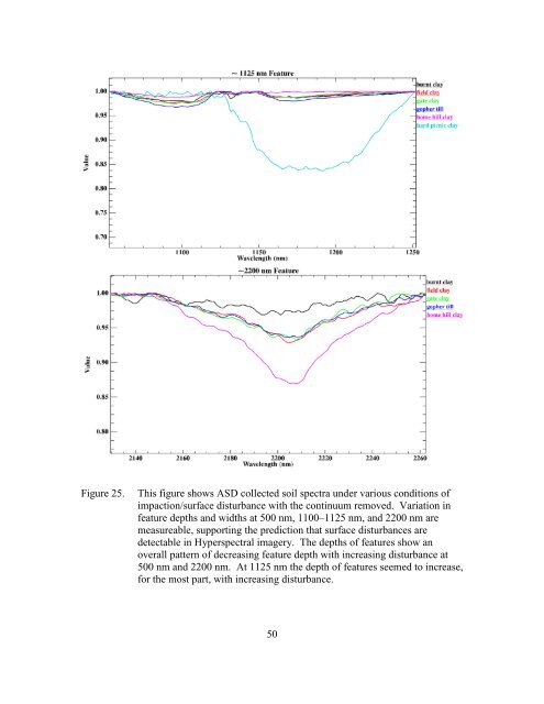
Figure 25. This figure shows ASD collected soil spectra under various conditions of impaction/surface disturbance with the continuum removed. Variation in feature depths and widths at 500 nm, 1100–1125 nm, and 2200 nm are measureable, supporting the prediction that surface disturbances are detectable in Hyperspectral imagery. The depths of features show an overall pattern of decreasing feature depth with increasing disturbance at 500 nm and 2200 nm. At 1125 nm the depth of features seemed to increase, for the most part, with increasing disturbance. 50
The absorption feature band depths for the ~500 nm, 1125 nm, and 2200 nm features are 0.0232, 0.0176, and 0.0304 for burnt clay (Table 1). The field road clay values were 0.052, 0.0193, 0.0745, gate clay values 0.057, 0.021, 0.0645, gopher till values 0.0419, 0.026, 0.073, home hill clay values 0.092, 0.0087, 0.137, and hard picnic area clay values 0.0805, 0.154, 0.000 (flat) are for 500 nm, 1125nm, and 2200 nm, respectively (Table 1). The continuum removed values are representative of the depths of the absorption features at each wavelength calculated using (5) and (6), and are thought to be associated with how the soil components are altered with various levels of disturbance. As previously mentioned, Clark and Roush (1984) discussed how the use of the continuum removed function allows one to analyze a spectrum that is not heavily influenced by the processes of other minerals in a mixture or those within the mineral itself. Therefore, the depths of the absorption features and the changes occurring amongst them must be related to some change in the intrinsic properties of the soils themselves, as was suggested by Prose (1985) and postulated by this study. Table 1. This table lists the absorption feature depths for each soil spectrum using the continuum removed function and the deepest portion of the feature. The values listed show changes in the depth of features for the same material under different disturbance conditions for wavelengths of ~500 nm, 1125 nm, and 2200 nm. The depths are ordered by least to greatest disturbance and show, for the most part, a trend of decreasing depth, increasing depth, and decreasing depth at 500 nm, 1125 nm, and 2200 nm, respectively. 51
- Page 19 and 20: LIST OF ACRONYMS AND ABBREVIATIONS
- Page 21 and 22: I. INTRODUCTION A study published b
- Page 23 and 24: II. THE PHYSICS BEHIND REMOTE SENSI
- Page 25 and 26: sensitive a given sensor is to diff
- Page 27 and 28: Figure 3. From Green et al. (1998),
- Page 29 and 30: analyzing imagery spectra, it is mo
- Page 31 and 32: After data have been converted to r
- Page 33 and 34: Collins et al. (1997) was able to s
- Page 35 and 36: These purposes include, but are not
- Page 37 and 38: III. DESERT ECOSYSTEM CHARACTERISTI
- Page 39 and 40: sagebrush of Utah, Montana, and the
- Page 41 and 42: in desert regions include argids, o
- Page 43 and 44: 2. Biological Soil Crusts (BSCs) Bi
- Page 45 and 46: 2004), especially in cases where ma
- Page 47 and 48: IV. STUDY SITES The focus area of t
- Page 50 and 51: Figure 13. This figure illustrates
- Page 52 and 53: Following the uplift that occurred
- Page 54 and 55: the Mazourka Canyon OHV park betwee
- Page 56 and 57: wavelengths being analyzed to obtai
- Page 58 and 59: 2. Field Spectroscopy An Analytical
- Page 60 and 61: A spectral library was then built a
- Page 62 and 63: after atmospherically correcting th
- Page 64 and 65: where: is the mean corrected and no
- Page 66 and 67: also be seen in Figure 23. The leve
- Page 68 and 69: Figure 24. This figure is a compari
- Page 72 and 73: Looking at Figure 25 it is apparent
- Page 74 and 75: A. IMAGERY DERIVED ENDMEMBERS The i
- Page 76 and 77: Figure 28. The above shows some of
- Page 78 and 79: spectrometer, reflectance values we
- Page 80 and 81: such an inference can be made (Ben-
- Page 82 and 83: While this is lower than the hoped
- Page 84 and 85: While the lower value would initial
- Page 86 and 87: Figure 33. This figure shows the ad
- Page 88 and 89: Inset C of Figure 35 is the same da
- Page 90 and 91: However, the presences of BSCs are
- Page 92 and 93: A B C Figure 37. Inset A shows the
- Page 94 and 95: A B C Figure 38. Inset A shows a co
- Page 96 and 97: differences in the studies by other
- Page 98 and 99: small concentrations making them un
- Page 100 and 101: area making it possible to tell wha
- Page 102 and 103: Clark, R. N., Swayze, G. A., Livo,
- Page 104 and 105: Kruse, F. A., Boardman, J. W., and
- Page 106 and 107: Sharp, R. P., and Glazner, A. F., (
- Page 108: INITIAL DISTRIBUTION LIST 1. Defens
Figure 25. This figure shows ASD collected soil spectra under various conditions of<br />
impaction/surface disturbance with <strong>the</strong> continuum removed. Variation in<br />
feature depths and widths at 500 nm, 1100–1125 nm, and 2200 nm are<br />
measureable, supporting <strong>the</strong> prediction that surface disturbances are<br />
detectable in Hyperspectral imagery. The depths of features show an<br />
overall pattern of decreasing feature depth with increasing disturbance at<br />
500 nm and 2200 nm. At 1125 nm <strong>the</strong> depth of features seemed <strong>to</strong> increase,<br />
<strong>for</strong> <strong>the</strong> most part, with increasing disturbance.<br />
50


