Low-Frequency, All-Sky Imaging with the PAPER Array Using AIPY
Low-Frequency, All-Sky Imaging with the PAPER Array Using AIPY
Low-Frequency, All-Sky Imaging with the PAPER Array Using AIPY

You also want an ePaper? Increase the reach of your titles
YUMPU automatically turns print PDFs into web optimized ePapers that Google loves.
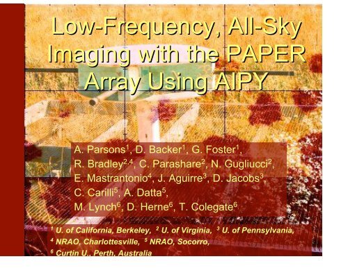
<strong>Low</strong>-<strong>Frequency</strong>, <strong>All</strong>-<strong>Sky</strong><br />
<strong>Imaging</strong> <strong>with</strong> <strong>the</strong> <strong>PAPER</strong><br />
<strong>Array</strong> <strong>Using</strong> <strong>AIPY</strong><br />
A. Parsons 1 , D. Backer 1 , G. Foster 1 ,<br />
R. Bradley 2,4 , C. Parashare 2 , N. Gugliucci 2 ,<br />
E. Mastrantonio 4 , J. Aguirre 3 , D. Jacobs 3 ,<br />
C. Carilli 5 , A. Datta 5 ,<br />
M. Lynch 6 , D. Herne 6 , T. Colegate 6<br />
1 U. of California, Berkeley, 2 U. of Virginia, 3 U. of Pennsylvania,<br />
4 NRAO, Charlottesville, 5 NRAO, Socorro,<br />
6 Curtin U., Perth, Australia
The <strong>PAPER</strong> Architecture<br />
Flexible FPGA-based<br />
Packetized Correlator<br />
Full-Stokes<br />
Large # Ants (scalable)!<br />
Wide Band (up to 200 MHz)!<br />
2048 Channel Polyphase<br />
Filter Banks<br />
4-bit Cross-Multipliers<br />
Non-tracking Crossed Dipoles<br />
Wide Bandwidth (125-205 MHz)!<br />
Movable (unburied TV cable)!<br />
Smooth Beam<br />
<strong>AIPY</strong>: Model-based <strong>Imaging</strong>/Calibration<br />
Bootstrap <strong>Imaging</strong>/Calibration<br />
W Projection, Multi-frequency Syn<strong>the</strong>sis<br />
Python-Based, Ties in MIRIAD, HEALPIX<br />
Measurement Equation-based Parameter Fit
<strong>PAPER</strong> Antennas/Analog Electronics<br />
Developed by <strong>the</strong> Charlottesville (NRAO,UVA) Team<br />
! Smooth beam (spatially and spectrally)<br />
! Gain sensitive to ambient temperature
<strong>PAPER</strong>/CASPER Packetized Correlator<br />
Two Dual<br />
500 Msps<br />
ADCs + IBOB<br />
Berkeley Wireless Research Center's BEE2
Two Calibration/<strong>Imaging</strong> Paths...<br />
Parameter Space:<br />
Bootstrap: Direct, fast, imperfect<br />
“Sometimes you can't get started because you can't get started” – Don Backer<br />
Model-Fit: Clean, correct, expensive<br />
<strong>AIPY</strong>: Astronomical<br />
stronomical<br />
Interferometry nterferometry in Python Python<br />
an open-source toolkit targeting<br />
low-frequency interferometry<br />
http://pypi.python.org/pypi/aipy
<strong>AIPY</strong> is:<br />
<strong>AIPY</strong> isn't:<br />
What <strong>AIPY</strong> Is (and Isn't)!<br />
! A module adding tools for interferometry to Python (not visa versa)!<br />
! An amalgam of pure-Python and wrappers around C++ and Fortran<br />
! Object-Oriented<br />
! A collection of low- to mid-level operations (you write <strong>the</strong> program)!<br />
! A toolkit (i.e. a grocery store, not a restaurant)!<br />
! In beta release (frequent updates/bug-fixes/changes)!<br />
! A solution (it just helps you find it)!<br />
! A one-stop shop (it makes use of o<strong>the</strong>r open-source projects)!<br />
! A replacement for o<strong>the</strong>r interferometry packages<br />
! Wedded to a file format (but only MIRIAD-UV, FITS currently supported)!<br />
Philosophical Pedantry:<br />
! Follow <strong>the</strong> (abbreviated) Zen of Python:<br />
! Explicit is better than implicit<br />
! Simple is better than complex<br />
! Complex is better than complicated<br />
! Special cases aren't special enough to break <strong>the</strong> rules<br />
! Practicality beats purity<br />
! There should be one (and preferably only one) obvious way to do it,<br />
although that way may not be obvious at first unless you're Dutch<br />
! Now is better than never<br />
! In <strong>the</strong> face of ambiguity, refuse <strong>the</strong> temptation to guess<br />
! Don't handicap <strong>the</strong> programmer; allow <strong>the</strong>m all <strong>the</strong> rope <strong>the</strong>y want<br />
! Don't hide data; return it (or at least grant access) at every turn
MODULES:<br />
ant/sim/fit<br />
const<br />
coord<br />
deconv<br />
healpix<br />
img<br />
loc<br />
map<br />
miriad<br />
optimize<br />
src<br />
----3rd party---ephem<br />
pyfits<br />
numpy<br />
pylab/matplotlib<br />
The Toolbox<br />
geometry, phase / gain, amplitude / parameter fitting<br />
physical constants<br />
coordinate transforms (eq, ec, ga, precession, etc.)!<br />
deconvolution (clean, lsq, mem, anneal)!<br />
wrapper around healpix C++ (Max-Planck-Institut)!<br />
imaging (gridding/weighting, W projection, beam calc)!<br />
machinery for importing user-defined Antenna<strong>Array</strong>s<br />
generation of all-sky maps, faceting<br />
interface to MIRIAD files<br />
parameter fitting, optimization code<br />
lists of known sources and parameters<br />
-----------------------------------------------------------------------------astrometry<br />
(relied upon heavily)!<br />
reading/writing FITS files<br />
numerical python (fundamental to everything)!<br />
plotting, map projection<br />
and example scripts for:<br />
manipulating/visualizing MIRIAD files, flagging RFI, filtering out crosstalk,<br />
fitting parameters, simulating arrays, making/viewing all-sky maps,<br />
phasing to/filtering out sources, imaging, etc.
Antenna<strong>Array</strong><br />
! set_jultime(...)!<br />
! gen_phs(...)!<br />
! gen_uvw(...)!<br />
! sim(...)!<br />
Antenna<br />
! x,y,z<br />
! dly,off<br />
! bp_r,bp_i<br />
Beam<br />
! response(...)!<br />
! <br />
Building a Simulator<br />
Antenna<br />
! x,y,z<br />
! dly,off<br />
! bp_r,bp_i<br />
RadioFixedBody<br />
! compute(...)!<br />
! ra,dec<br />
! str,index<br />
! angsize<br />
SrcCatalog<br />
! compute(...)!<br />
! get_crd(...)!<br />
YourModule.py<br />
! get_aa(...)!<br />
! get_catalog(...)!<br />
RadioSpecial<br />
! compute(...)!<br />
! str,index<br />
! angsize
<strong>PAPER</strong> Deployments<br />
PGB: <strong>PAPER</strong>, Green Bank PWA: <strong>PAPER</strong>, Western Australia<br />
! PGB-4: 2004-6, ants w/o flaps, 1 brd correlator<br />
! PGB-8: 2006-8, upgraded ants, packet correlator<br />
! PGB-16: 2008-?, testing & characterization<br />
! Prototype facility for PWA deployments<br />
38:25:59.24 N<br />
-79:51:02.1 W<br />
Green Bank, WV<br />
! PWA-4: 2007, ants w/o flaps, 1 brd correlator<br />
! (PWA-32): 2009, ants w/ flaps, packet correlator<br />
! (PWA-128): 2010?<br />
! <strong>Low</strong>-RFI, full-capability facility<br />
-26:44:12.74 S<br />
116:39:59.33 E<br />
Boolardy, WA
Antenna Configuration<br />
! Inner circle is PWA-4 configuration<br />
! Outer circle is PGB-8 configuration<br />
! Shaded circles have radius = 10x elevation (dark is negative)!
Sample Data: 1 Day, 1 Baseline, PGB<br />
Fringes (Cas,Cyg,Sun)!<br />
Phase Amplitude (log)!<br />
Crosstalk<br />
Intermittent TX<br />
Beating sources<br />
Satellite TX<br />
TV/Aircraft TX
1-D “Delay” <strong>Imaging</strong><br />
XRFI:<br />
! Remove model sky<br />
! Statistical thresholding<br />
! Manual flagging<br />
DELAY TF:<br />
! iFFT of passband<br />
! Convolved by<br />
“delay beam”<br />
1D CLEAN:<br />
! Compensate for<br />
holes in passband<br />
! Retain passband<br />
shape for self-cal
Delay/Delay-Rate<br />
Transform<br />
! 1 hour of data <strong>with</strong> Cas A, Cyg A, Tau A<br />
! Phase to a source (here, Cas A)!<br />
! FFT of frequency axis = “Delay Image”<br />
! FFT of time axis = “Delay/Delay-Rate”<br />
! Cas A is confined to a region near origin<br />
! PSF determined by bandpass + time variabliity<br />
! Can recover bandpass + beam functions
Delay/Delay-Rate Transform<br />
! Two sources can show up at same delay for a given baseline<br />
! Over a time interval (say, 1 hr), can be differentiated by fringe rates (see below)!<br />
! To prevent excessive blurring (changing fringe rate w/ time) best to phase to source before filtering<br />
! Clean delay axis before iFFT of time axis<br />
! Clean fringe rate axis to account for flagging of entire integrations<br />
! Top to bottom: 3 baseline orientations<br />
! Left to right: delay bins, delay-rate bins, and combined<br />
filter bins<br />
! DDR filters have 2 lobes of response: one that tracks<br />
your source, one that sweeps across <strong>the</strong> sky
Recovering Bandpass and Beam<br />
! Top plot:<br />
Kernels from DDR Transform<br />
! '+' = uncleaned bandpass recovered<br />
! heavy dots = cleaned bandpass<br />
! light dots = autocorr for comparison<br />
! Bottom plot:<br />
! '+' = uncleaned delay image<br />
! line = cleaned delay image<br />
! Cas A response versus time, Cyg A removed, 143<br />
MHz (top) and 165 MHz (bottom)!<br />
! '+' = beam response recovered using delay filter<br />
! dots = beam response recovered using DDR<br />
! lines = prediction of beam model
Modeling Beam of Dipole + Flaps<br />
138 MHz 156 MHz 174 MHz<br />
40dB zenith to horizon, 60 degree FWHM<br />
Smooth spatially and vs. frequency
Model Beam vs. Source Strengths<br />
Black: response toward Cas A<br />
Blue: response toward Cyg A<br />
Cyan: response toward Tau A<br />
Green: response toward Vir A<br />
Red: response toward Sun
<strong>Imaging</strong> <strong>with</strong> Non-Tracking Beams<br />
! Only possible to weight for one track through primary beam<br />
! Dirty beam weighted for phase center imperfectly deconvolves away from center<br />
! Can evade problem <strong>with</strong> snapshot imaging<br />
Position-Dependent Weighting in Data Dirty Beam <strong>with</strong> Incorrect Weighting
138.8-174.0 MHz PWA-4/PGB-8<br />
! Scale: log(Jy/beam)!<br />
! black->cyan = -1 to 1<br />
! yellow >= 2, red >= 3<br />
! Equatorial Mollweide Projection, RA=0 on right<br />
! Confusion at 80mJy/beam RMS at positive dec<br />
! Sun at (1:10,+7:27), removed <strong>with</strong> DDR filter<br />
! Cyg,Cas,Vir,Tau peeled <strong>with</strong> ionospheric-dependent<br />
solutions.<br />
<strong>Using</strong>:<br />
8 Antennas at pos dec, 4 at negative<br />
3 days of data, 14s integrations<br />
W projected, ~15 deg phase centers
! 1 day of 8-element single polarization data<br />
! Spans 138.8 to 174.0 MHz<br />
! Model subtraction of Cyg,Cas,Vir,Crab<br />
! Fit for ionospheric defraction<br />
! Delay/F subtraction of Sun<br />
! Map has constant flux scale<br />
! Changing noise level due to beam response<br />
150 MHz PGB-8
Tsys = 250K<br />
# FoV = 0.425 strradians<br />
$ 0 = 162.5 MHz<br />
%$ = 35.2 MHz<br />
PGB-8 Thermal Noise Map<br />
# bm<br />
Nant &int RMS Noise Map, log10(Jy/bm)!<br />
= 2.2e-5 strradians<br />
= 8 antennas<br />
= 3 day observing<br />
= 3.5 hrs/pointing<br />
Integrations added <strong>with</strong> alternating signs<br />
RA,DEC = 12:00, 40:00<br />
< "T > = 625 mK (10 mJy/bm)!
PGB-8 System Temperature<br />
Tsys (and predicted synchrotron)!<br />
Tsky (confusion + synchrotron)!<br />
Thermal noise (3 day integration)!<br />
<strong>Using</strong> RMS pixel values from 4 patches near<br />
RA=12:00,DEC=40:00 as a function of frequency, we<br />
determine a perceived Tsky and <strong>the</strong>rmal noise level.<br />
Backing out integration, this gives us Tsys<br />
Tsky<br />
Thermal noise
Power Spectra and Foregrounds<br />
“Beware <strong>the</strong> Jabberwock, my son!<br />
The jaws that bite, <strong>the</strong> claws that catch!”<br />
-Lewis Carrol (1872)!<br />
21 cm EoR (z=9.5)!<br />
Power spectra at 146.6, 155.7, 164.5, and 173.3 MHz<br />
(top to bottom w/ error bars), from 4 fields near<br />
RA=12:00,DEC=40:00.<br />
Point source dominated, starting to see synchrotron<br />
at lower frequencies, wavemodes<br />
Galactic Synchrotron<br />
Confusion Noise<br />
Galactic Free-Free<br />
Extragalactic Free-Free<br />
21 cm EoR (z=9.5)!<br />
CMB Background
Summary<br />
!16 antennas deployed in PGB, 32 in PWA this fall<br />
!Analog system working well, going into production<br />
!Packetized Correlator enabling build-out in staged deployments<br />
! Working on QADC to lower digitizing cost, reducing to 100 MHz BW<br />
! <strong>Low</strong>ering integration time to ~8s<br />
!<strong>AIPY</strong>-based processing pipeline maturing<br />
! Available at http://pypi.python.org/pypi/aipy<br />
! Working on cluster/parallel computing<br />
!Ionospheric refraction noticeable in data, compensated per source<br />
!Have a confusion/synchrotron-limited map (8.4K), ready for next tier of foreground removal<br />
!Thermal noise in map (600 mK) continuing to integrate down<br />
!Source removal currently limited by primary beam model<br />
! <strong>Using</strong> satellites to characterize per-antenna beam shapes<br />
!Have not started investigating polarization or galactic synchrotron
Confusion Noise<br />
Need to balance array configuration between resolving and removing confusing sources (long<br />
baselines), and optimizing for a power spectrum detection (concentrated core). Below, a map <strong>with</strong> no<br />
sources removed (left) and <strong>with</strong> <strong>the</strong> top 5 sources removed (right), <strong>with</strong> corresponding pixel histograms.
Ionosphere<br />
Time scale: 10s Length scale: few km Refraction scale: few arcminute<br />
Pushes up data rates, need for instantaneous UV coverage (snapshot imaging)!<br />
Avoid dawn/dusk when ionosphere is highly variable<br />
Affects degree to which confusion noise can be suppressed
Ionosphere<br />
Time scale: 10s Length scale: few km Refraction scale: few arcminute<br />
Pushes up data rates, need for instantaneous UV coverage (snapshot imaging)!<br />
Avoid dawn/dusk when ionosphere is highly variable<br />
Affects degree to which confusion noise can be suppressed<br />
Black: Cas A, Magenta: Cyg A, 3 days of data, nighttime is shaded
38:25:59.24 N<br />
-79:51:02.1 W<br />
Green Bank, WV
38:25:59.24 N<br />
-79:51:02.1 W<br />
Green Bank, WV
-26:44:12.74 S<br />
116:39:59.33 E<br />
Boolardy, WA
-26:44:12.74 S<br />
116:39:59.33 E<br />
Boolardy, WA
Radio <strong>Frequency</strong> Interference<br />
Solution 1: Discretion is <strong>the</strong> better part of valor (run away)!<br />
Solution 2: Statistical thresholding of raw data<br />
Solution 3: Manually flag contaminated channels<br />
Solution 4: Delay/Delay-Rate Filtering<br />
Solution 5: Statistical thresholding after model subtraction<br />
Boolardy, Australia Site Characterization<br />
Blue:Peak, Green:Average, Red:Minimum<br />
Light: PWA, 3 days of data<br />
Dark: PGB, 3 days of data
Interferometry Fundamentals<br />
Our Parameterized Measurement Equation:<br />
Flat Field (Small Angle) Approximation:<br />
! (u,v) coordinates represent <strong>the</strong> Fourier transform of <strong>the</strong> angular sky coordinates (l,m)!<br />
! Angular power spectrum directly measured in UV (visibility) domain<br />
! Inverse 2D FFT of gridded UV visibilities yields dirty image (convolved <strong>with</strong> syn<strong>the</strong>sized<br />
PSF)!<br />
! Syn<strong>the</strong>sized PSF is inverse 2D FFT of visibility weights
Comparing <strong>with</strong> O<strong>the</strong>r Experiments<br />
MWA <strong>PAPER</strong> LOFAR 21CMA<br />
Advantages/Philosophies:<br />
! Hands on: collect data early, address problems as <strong>the</strong>y are encountered in data<br />
! Flexibility to adapt to new <strong>the</strong>ory and new knowledge about foregrounds<br />
! Optimize smoothness of parameter space to allow faster, more precise fitting<br />
! Wide simultaneous bandwidth, full correlation of large numbers of antennas<br />
! Both fully functional prototype environment and low RFI location<br />
Disadvantages:<br />
! Collecting area<br />
! Simulation<br />
Unsure:<br />
! Spectral resolution vs. bandwidth<br />
! Group size
Actual<br />
Primary<br />
Beam<br />
Restricted<br />
Visibilities<br />
<strong>Sky</strong>-Vis Relationships<br />
<strong>Sky</strong> |Vis| ø(Vis)!<br />
Implications for<br />
measuring PS<br />
Field of view (FoV)<br />
determines coherence region<br />
in visibility domain.<br />
Signal strength depends on<br />
FoV<br />
For incoherent signal<br />
summation, scaling of SNR <strong>with</strong><br />
# samples depends on SNR of<br />
samples:
Sample UV Optimized for 3 Scales<br />
Nested Triangular Configuration<br />
<strong>with</strong> Outlying Calibrators<br />
UV coverage Dirty Beam
Slices Through Image<br />
Virgo A<br />
Galactic Plane/Her A<br />
Confusion Sun Confusion<br />
2008 May 13 Harvard-Smithsonian: 21cm Cosmology 38
Power Spectra<br />
What an interferometer measures:<br />
Related measures used in literature:
Sensitivity in Visibility Domain<br />
Tsky ~ 160K<br />
#beam ~ 60 deg x 60 deg<br />
%$ ~ 5 MHz<br />
#patch ~ 10 deg x 10 deg<br />
Nsamples ~ 81 baselines<br />
&s ~ 40 min (varies <strong>with</strong> patch size and baseline orientation)!<br />
To hit SNR~1 in a UV pixel:<br />
' ~ 2 months for 0.5 mK<br />
Minimum to constrain cosmic variance:<br />
- 3 sigma detection ~ 9 pixels around circle.<br />
- <strong>Using</strong> nested triangles <strong>with</strong> 3x3 antennas at each virtex,<br />
~ 64 antennas (being clever).<br />
- Want to sample multiple rings to select for<br />
shape of power spectrum, so more like 128 antennas.<br />
- Need calibrator/imaging antennas, so more like<br />
160 antennas.<br />
BUT...<br />
** UV pixel sampled is frequency dependent,<br />
undermining ability to subtract foregrounds.<br />
!^<br />
v<br />
u
What we can learn in first experiments:<br />
! Time of EoR degenerately constrains<br />
What We Can Learn<br />
! Dark Energy/Dark Matter (time for structure to collapse) + star formation rate<br />
! Confirm inside-out structure formation<br />
! X-ray heating by first quasars<br />
What we can learn <strong>with</strong> SKA-class study:<br />
! Matter power spectrum through Dark Ages<br />
! Constrains dark energy, dark matter<br />
(growth factor in collapse)!<br />
! Constrains time of radiation-matter<br />
equality (transfer function)!<br />
! Geometry of Reionization<br />
! Star formation<br />
! Galaxy formation<br />
! Supermassive black hole formation<br />
! Feedback of reionization on<br />
structure formation<br />
“Richest of all datasets”
Interaction Distance Scale (log)!<br />
Evolution of Perturbations<br />
Density Perturbation (log)!<br />
Inflationary Radiation Dominated Matter Dominated...<br />
Time (log)!<br />
Recombination<br />
Matter-Radiation Equality
Simulated Power Spectra
21 cm Spin Temp<br />
Wouthuysen Field Effect
Bounds on EoR (6
Raw Sensitivity in Image Domain<br />
Tsys = Tsky + Trx ~ 170K + 110K<br />
%$ ~ 1 MHz<br />
N ~ 256<br />
Aeff ~ 2<br />
#obs ~ 1 to 0.1 degrees<br />
For necessary sensitivity:<br />
' ~ 1 month for 1 mK at<br />
1 degree (l ~ 100)!<br />
or more likely:<br />
' ~ 10 yrs for 1 mK at<br />
0.1 degree (l ~ 1000)!<br />
Galactic Synchrotron<br />
Confusion Noise<br />
Galactic Free-Free<br />
Have added flaps to<br />
! increase collecting area<br />
! reduce sky temp<br />
(z=9.5)!<br />
! suppress sidelobes of sources<br />
EoR cm<br />
! supress RF 21<br />
Extragalactic Free-Free<br />
CMB Background
Challenge: Starting from Scratch<br />
The Problem:<br />
“Sometimes you can't get started because you can't get started” – Don Backer<br />
! Self-calibration needs single-source data<br />
! Source isolation requires calibration<br />
! Parameter fitting needs a good starting guess<br />
! How do we get to first base?<br />
Bootstrapping:<br />
! Direct, imperfect, iterative<br />
! Do not rely (excessively) on priors<br />
! Take advantage of wide bandwidth<br />
! Address degeneracies one at a time
Polarized Galactic Synchrotron<br />
150 MHz Power Spectrum Predicted<br />
from Komolgorov Turbulence<br />
Faraday Rotation Screen:<br />
! Smooth <strong>with</strong> frequency, but improperly calibrated linear<br />
polarization can produce frequency-dependent structure.<br />
! Smooth power spectrum can allow fur<strong>the</strong>r rejection.<br />
! Need a factor of 1000 suppression<br />
325 MHz Measured Polarization