value averaging and the automated bias of ... - Cass Knowledge
value averaging and the automated bias of ... - Cass Knowledge
value averaging and the automated bias of ... - Cass Knowledge

You also want an ePaper? Increase the reach of your titles
YUMPU automatically turns print PDFs into web optimized ePapers that Google loves.
VALUE AVERAGING AND THE AUTOMATED BIAS OF PERFORMANCE<br />
MEASURES<br />
Abstract:<br />
Value <strong>averaging</strong> is a formula investment strategy which can be shown to achieve a lower<br />
average cost <strong>and</strong> higher IRR than alternative strategies. However, in contrast to previous studies,<br />
this paper shows that this does not lead to higher expected pr<strong>of</strong>its. Instead an “<strong>averaging</strong> down”<br />
effect systematically <strong>bias</strong>es <strong>the</strong> IRR up <strong>and</strong> <strong>the</strong> average purchase cost down. The same <strong>bias</strong><br />
applies to a wide class <strong>of</strong> investment strategies (including dollar cost <strong>averaging</strong>) where <strong>the</strong><br />
amount invested in each period is negatively correlated with <strong>the</strong> return made to date.<br />
This version: 18 May 2010<br />
Preliminary draft: comments welcome, but please do not cite without author’s permission<br />
Simon Hayley<br />
<strong>Cass</strong> Business School<br />
00-44-(0)20-7040-0230<br />
1
1. Introduction<br />
Value <strong>averaging</strong> (VA) is a formula investment strategy which can be shown to achieve lower<br />
average costs <strong>and</strong> higher IRRs than alternative strategies. However, in contrast to previous<br />
studies, this paper will show that this does not lead to higher expected pr<strong>of</strong>its.<br />
VA is in some respects similar to dollar cost <strong>averaging</strong> (DCA), which is <strong>the</strong> practice <strong>of</strong> building up<br />
investments gradually over time in equal dollar amounts, ra<strong>the</strong>r than investing <strong>the</strong> desired total in<br />
one lump sum. Table 1 compares DCA with a strategy <strong>of</strong> buying equal numbers <strong>of</strong> shares each<br />
period (ESA). The DCA strategy invests $100 each period, whereas ESA purchases 100 shares<br />
each period. Shares initially cost $1, but <strong>the</strong> DCA strategy buys more shares as prices fall. Thus<br />
DCA achieves a lower average share price than ESA. Conversely, if prices rose, <strong>the</strong>n DCA would<br />
purchase fewer shares in later periods, again achieving a lower average cost.<br />
Table 1 Equal Share Amounts (ESA) Dollar Cost Averaging (DCA) Value Averaging (VA)<br />
Period Price<br />
Shares<br />
bought<br />
Invest-<br />
ment<br />
($)<br />
Portfolio<br />
($)<br />
Shares<br />
bought<br />
2<br />
Invest-<br />
ment<br />
($)<br />
Portfolio<br />
($)<br />
Shares<br />
bought<br />
Invest-<br />
ment<br />
($)<br />
Portfolio<br />
($)<br />
1 1.00 100 100 100 100 100 100 100 100 100<br />
2 0.90 100 90 171 111 100 180 122 110 200<br />
3 0.80 100 80 216 125 100 240 153 122 300<br />
Total 300 270 336 300 375 332<br />
Average cost: 0.900 0.893 0.886<br />
Proponents <strong>of</strong> DCA argue that as it reduces <strong>the</strong> average purchase cost, it must generate higher<br />
returns. By contrast, previous academic research has long shown that despite its lower average<br />
cost, DCA is a sub-optimal strategy. Never<strong>the</strong>less, it remains very popular among investors <strong>and</strong><br />
is widely recommended in <strong>the</strong> financial press <strong>and</strong> popular finance literature.<br />
The motivation for <strong>value</strong> <strong>averaging</strong> (VA) is similar. In contrast to DCA, VA has a target increase in<br />
portfolio <strong>value</strong> each period (assumed in Table 1 to be a rise <strong>of</strong> $100 per period). The investor<br />
must invest whatever amount is necessary in each period to meet this target. Like DCA, VA<br />
purchases more shares after a fall in prices, but <strong>the</strong> response is more sensitive: in this example<br />
VA buys 122 shares in period 2, compared to 111 for DCA <strong>and</strong> 100 for ESA. As Table 1 shows,<br />
<strong>the</strong> more aggressive response <strong>of</strong> VA to shifts in <strong>the</strong> share price results in an even lower average<br />
purchase cost. Again, this is true whe<strong>the</strong>r prices rises or fall.<br />
In contrast to DCA, VA is a relatively recent invention (first suggested by Edelson, 1988) <strong>and</strong> <strong>the</strong><br />
only studies assessing its performance recommend it on <strong>the</strong> grounds that it results in a higher<br />
IRR (Edelson (1991), Marshall (2000, 2006)).<br />
Nei<strong>the</strong>r strategy claims to be taking advantage <strong>of</strong> market inefficiencies. Indeed, simulations<br />
appear to show that <strong>the</strong>se trading rules bring benefits even when prices follow a r<strong>and</strong>om walk.<br />
Moreover, both are fixed rules which pre-commit investors, allowing <strong>the</strong> investor no discretion<br />
once committed to <strong>the</strong> strategy. As a result, both are subject to <strong>the</strong> criticisms set out by<br />
Constantinides (1979), who showed that strategies which pre-commit investors must be expected<br />
to be dominated by strategies which allow investors to react to incoming news.<br />
DCA may also seem to improve diversification by making many small purchases but, as Rozeff<br />
(1994) notes, <strong>the</strong> result is that overall pr<strong>of</strong>its are most sensitive to returns in <strong>the</strong> later part <strong>of</strong> <strong>the</strong><br />
period, when <strong>the</strong> investor is nearly fully invested. Earlier returns are given correspondingly little<br />
weight, since <strong>the</strong> investor <strong>the</strong>n holds mainly cash. Better diversification is achieved by investing in<br />
one initial lump sum, <strong>and</strong> thus being equally exposed to <strong>the</strong> returns in each sub-period. Milevsky
<strong>and</strong> Posner (1999) show that it is always possible to construct a constant proportions<br />
continuously rebalanced portfolio which will stochastically dominate DCA in a mean-variance<br />
framework, <strong>and</strong> that for typical levels <strong>of</strong> volatility <strong>and</strong> drift <strong>the</strong>re will be a static buy <strong>and</strong> hold<br />
strategy which dominates DCA.<br />
Studies based on historical data have found that investing in one lump sum has generally given<br />
better mean-variance performance than DCA. These include Knight <strong>and</strong> M<strong>and</strong>ell (1992/93),<br />
Williams <strong>and</strong> Bacon (1993), Rozeff (1994) <strong>and</strong> Thorley (1994). This inefficiency may seem at<br />
odds with DCA’s lower average costs, but Hayley (2009) shows that comparing <strong>the</strong> average cost<br />
achieved by DCA with <strong>the</strong> average price is misleading: it implicitly compares DCA with a strategy<br />
which uses perfect foresight to invest more when prices are about to fall <strong>and</strong> less when <strong>the</strong>y are<br />
about to rise. It is only because <strong>of</strong> this <strong>bias</strong> that DCA appears to <strong>of</strong>fer higher returns.<br />
Proponents <strong>of</strong> VA tend to focus not on its lower average cost, but on <strong>the</strong> fact that it achieves a<br />
higher IRR than alternative strategies. Higher IRRs might seem to imply higher expected pr<strong>of</strong>its,<br />
but we demonstrate here that VA systematically <strong>bias</strong>es up its IRR without increasing expected<br />
pr<strong>of</strong>its.<br />
The structure <strong>of</strong> this paper is as follows: section 2 demonstrates that in contrast to proponents’<br />
claims, VA cannot expect to generate excess returns when prices follow a r<strong>and</strong>om walk. This is<br />
confirmed by <strong>the</strong> Monte Carlo simulations presented in Section 3, which show that DCA <strong>and</strong> VA<br />
generate lower average purchase costs <strong>and</strong> higher IRRs, but do not increase average pr<strong>of</strong>its. We<br />
<strong>the</strong>n investigate why average purchase costs (Section 4) <strong>and</strong> IRRs (Section 5) are systematically<br />
<strong>bias</strong>ed by <strong>the</strong>se formula strategies. Section 6 briefly considers cashflow management <strong>and</strong> risk<br />
issues. Conclusions are drawn in <strong>the</strong> final section.<br />
2. Expected Pr<strong>of</strong>its<br />
In <strong>the</strong> analysis below we assume that investors do not believe that <strong>the</strong>y can forecast market<br />
prices - in effect <strong>the</strong>y assume that prices follow a r<strong>and</strong>om walk. However, we should stress that<br />
this is a statement about investors’ ex ante expectations, <strong>and</strong> does not imply any presumption<br />
that markets are in fact weak form efficient. The key point in this context is that VA, like DCA, will<br />
only ever be an attractive strategy for investors who do not believe that <strong>the</strong>y can forecast shortterm<br />
price movements. These strategies commit investors to invest a specified amount no matter<br />
what <strong>the</strong>y expect in <strong>the</strong> coming period – those who feel that <strong>the</strong>y can forecast short-term price<br />
movements will reject this <strong>and</strong> follow o<strong>the</strong>r strategies instead.<br />
We also assume that this r<strong>and</strong>om walk has zero drift. This too is a statement about investors’ ex<br />
ante expectations ra<strong>the</strong>r than about markets <strong>the</strong>mselves. Investors presumably believe that over<br />
<strong>the</strong> medium term <strong>the</strong>ir chosen securities will generate an attractive return, but <strong>the</strong>y must also<br />
believe that <strong>the</strong> return over <strong>the</strong> short term (while <strong>the</strong>y are using DCA or VA to build up <strong>the</strong>ir<br />
position) is likely to be small. Investors who expect significant returns over <strong>the</strong> short term would<br />
clearly prefer to invest immediately in one lump sum ra<strong>the</strong>r than delay <strong>the</strong>ir investments by<br />
following a strategy which invests gradually. Marshall (2000) suggests that VA boosts returns<br />
even in a r<strong>and</strong>om walk with zero drift.<br />
The assumption <strong>of</strong> zero drift need not imply a loss <strong>of</strong> generality, since drift could be incorporated<br />
into this framework by defining prices not as absolute market prices, but as prices relative to a<br />
numeraire which appreciates at a rate which gives a fair return for <strong>the</strong> risks inherent in this asset<br />
(pi*=pi/(1+r) i , where r reflects <strong>the</strong> cost <strong>of</strong> capital <strong>and</strong> a risk premium appropriate to this asset). We<br />
could <strong>the</strong>n assume that pi* has zero expected drift since investors who use VA or DCA will not<br />
believe that <strong>the</strong>y can forecast short-term relative asset returns: those who do would again reject<br />
trading strategies which forced <strong>the</strong>m to delay <strong>the</strong>ir purchases. The results derived below would<br />
3
continue to hold for pi*, with pr<strong>of</strong>its <strong>the</strong>n defined as excess returns compared to <strong>the</strong> risk-adjusted<br />
cost <strong>of</strong> capital. 1<br />
We consider investing over a series <strong>of</strong> n discrete periods. The price <strong>of</strong> <strong>the</strong> asset in each period i<br />
is pi. The alternative investment strategies differ in <strong>the</strong> quantity <strong>of</strong> shares qi that are purchased in<br />
each period. We evaluate pr<strong>of</strong>its at a subsequent point, after all investments have been made. If<br />
prices are <strong>the</strong>n pT, <strong>the</strong> expected pr<strong>of</strong>it made by any investment strategy is:<br />
<br />
n<br />
n<br />
piqi pTqi i1<br />
i1<br />
Our assumption <strong>of</strong> a r<strong>and</strong>om walk implies that future price movements (pT/pi) are independent <strong>of</strong><br />
<strong>the</strong> past <strong>value</strong>s <strong>of</strong> pi <strong>and</strong> qi. This gives us:<br />
<br />
n<br />
p<br />
iqi<br />
<br />
piqi<br />
i1<br />
<br />
<br />
<br />
<br />
<br />
p T<br />
p<br />
i<br />
<br />
<br />
<br />
<br />
<br />
4<br />
n<br />
i1<br />
<br />
But <strong>the</strong> r<strong>and</strong>om walk has zero drift, so E[pT/pi]=1 for all i <strong>and</strong> expected pr<strong>of</strong>its are zero. The<br />
amount piqi which is invested in each period is irrelevant: expected pr<strong>of</strong>its are zero for all <strong>the</strong><br />
investment strategies that we consider here. Total expected pr<strong>of</strong>it is <strong>the</strong> expected percentage<br />
capital gain between each period i <strong>and</strong> period T, multiplied by <strong>the</strong> amounts invested in each<br />
period. But our assumption <strong>of</strong> a driftless r<strong>and</strong>om walk implies that <strong>the</strong> expected gain is zero in all<br />
periods, so <strong>the</strong> timing <strong>of</strong> investments makes no difference. Against this background, <strong>the</strong> claim<br />
that VA <strong>and</strong> DCA can generate excess pr<strong>of</strong>its even in <strong>the</strong> absence <strong>of</strong> market inefficiencies is<br />
surprising.<br />
3. Monte Carlo Simulations<br />
Tables 2 <strong>and</strong> 3 shows <strong>the</strong> results <strong>of</strong> 10,000 simulations in which prices movements are<br />
distributed uniformly within <strong>the</strong> range +/-5% in each <strong>of</strong> five consecutive periods. The share price<br />
is initially $10. The four strategies compared here are:<br />
- ESA: buy 40 shares each period.<br />
- DCA: invest $400 each period.<br />
- VA: increase <strong>the</strong> portfolio <strong>value</strong> by $400 each period 2<br />
- Lump sum: purchase 200 shares in <strong>the</strong> first period.<br />
1 We must also assume that funds not yet needed for <strong>the</strong> VA strategy can be held in assets with <strong>the</strong> same<br />
expected return. This assumption is clearly generous to VA – if instead cash is held on deposit at lower<br />
expected return, <strong>the</strong>n VA’s expected return is clearly reduced by delaying investment.<br />
2 The VA strategy has one more parameter than DCA <strong>and</strong> ESA, since it requires us to specify both <strong>the</strong><br />
expenditure in <strong>the</strong> initial period <strong>and</strong> <strong>the</strong> target increase in portfolio <strong>value</strong> each period. In order to make <strong>the</strong><br />
DCA <strong>and</strong> VA results here as comparable as possible, we have set both <strong>the</strong>se figures to $400. Thus if prices<br />
remain constant <strong>the</strong> three strategies would have identical cashflows, with each investing $400 in every<br />
period. As shown in <strong>the</strong> previous section, this makes no difference to expected pr<strong>of</strong>its.<br />
(1)<br />
(2)
Table 2: Strategy Costs<br />
<strong>and</strong> Returns<br />
ESA DCA VA Lump Sum<br />
Avg.Cost ($) Mean 10.0009 9.9943 9.9842 10.0000<br />
Std. Error 0.0032 0.0032 0.0032 0.0000<br />
IRR (%) Mean -0.0159% -0.0034% 0.0133% -0.0182%<br />
Std. Error 0.0158% 0.0158% 0.0158% 0.0145%<br />
Pr<strong>of</strong>it ($) Mean 0.8706 0.8659 0.8648 1.0572<br />
Std. Error 0.6337 0.6331 0.6326 1.1589<br />
It might seem odd to use IRR to compare performance instead <strong>of</strong> more conventional measures<br />
such as <strong>the</strong> Sharpe ratio. In looking at IRRs we are following <strong>the</strong> methodology used by Edelson<br />
(1991) <strong>and</strong> Marshall (2000, 2006). Moreover, some <strong>of</strong> <strong>the</strong> key problems normally associated with<br />
<strong>the</strong> use <strong>of</strong> IRR (notably in real estate applications) are absent here: traded securities are likely to<br />
be highly divisible, in contrast to large real estate projects. Fur<strong>the</strong>rmore, <strong>the</strong> cashflows generated<br />
by real estate projects might have to be re-invested at very different yields, but our null<br />
hypo<strong>the</strong>sis here (that formula investment strategies generate no excess pr<strong>of</strong>its) would imply that<br />
surplus cashflows could be invested using different strategies at <strong>the</strong> same expected yield.<br />
Ultimately, we will argue that <strong>the</strong> IRR is a poor measure <strong>of</strong> pr<strong>of</strong>itability in this context, but this is<br />
for a more subtle reason. Phalippou (2008) notes that IRRs can be <strong>bias</strong>ed where <strong>the</strong> cashflows<br />
are endogenous to <strong>the</strong> IRR achieved to date, <strong>and</strong> that investment managers could thus<br />
manipulate <strong>the</strong>ir cashflows in order to boost <strong>the</strong>ir recorded IRRs. We show below that this <strong>bias</strong> is<br />
inherent in <strong>the</strong> VA <strong>and</strong> DCA strategies.<br />
Sharpe ratios are not used in this comparison because DCA <strong>and</strong> VA claim to achieve <strong>the</strong>ir<br />
benefits by strategically varying <strong>the</strong> cashflows involved. Thus if <strong>the</strong>se strategies do bring benefits,<br />
<strong>the</strong>y can only be assessed using a dollar-weighted performance measure such as IRR. By<br />
contrast, <strong>the</strong> time-weighted rates <strong>of</strong> return which are conventionally used in calculating Sharpe<br />
ratios (notably in GIPS methodology) deliberately strip away any cashflow effects, leaving only<br />
<strong>the</strong> relative performance <strong>of</strong> <strong>the</strong> assets involved. This would remove <strong>the</strong> effect <strong>of</strong> DCA <strong>and</strong> VA, so<br />
this is not a useful measure here. We will ultimately conclude that DCA <strong>and</strong> VA give zero<br />
expected excess pr<strong>of</strong>its, so we can infer that <strong>the</strong> Sharpe ratio will be zero in all <strong>the</strong> strategy<br />
simulations shown here, but in <strong>the</strong> meantime we investigate <strong>the</strong> IRR to avoid pre-judging <strong>the</strong><br />
issue <strong>and</strong> to show <strong>the</strong> nature <strong>of</strong> <strong>the</strong> <strong>bias</strong> involved.<br />
Table 3: Differences<br />
DCA -<br />
VA - Lump<br />
Between Strategies DCA - ESA Lump Sum DCA - VA VA - ESA Sum<br />
Avg.Cost ($) Mean -0.00668 -0.00574 0.01001 -0.01669 -0.01576<br />
Std. Error 0.00005 0.00317 0.00007 0.00011 0.00316<br />
IRR (%) Mean 0.0125% 0.0148% -0.0167% 0.0292% 0.0315%<br />
Std. Error 0.00013% 0.00646% 0.00018% 0.00028% 0.00646%<br />
Pr<strong>of</strong>it ($) Mean -0.00469 -0.1913 0.0011 -0.00579 -0.1924<br />
Std. Error 0.0149 0.636 0.0149 0.0279 0.637<br />
Table 3 shows that VA <strong>and</strong> DCA achieve highly significant reductions in average cost <strong>and</strong><br />
increases in IRR compared to both ESA <strong>and</strong> lump sum investment strategies. But <strong>the</strong>re are no<br />
significant differences in <strong>the</strong> pr<strong>of</strong>its made. As a robustness check, simulations were also run with<br />
price movements substantially more volatile (-25% to +25% per period) or less volatile (-1% to<br />
+1% per period) than those shown here. In each case DCA <strong>and</strong> VA recorded significantly higher<br />
IRRs <strong>and</strong> lower average costs, but no significant change in pr<strong>of</strong>its. We find <strong>the</strong> same if we use<br />
5
Marshall’s r<strong>and</strong>om investing strategy as our non-dynamic benchmark strategy (in place <strong>of</strong> <strong>the</strong><br />
lump sum <strong>and</strong> ESA strategies).<br />
Even on <strong>the</strong> assumption <strong>of</strong> a driftless r<strong>and</strong>om walk, where we know that <strong>the</strong> ex ante expected<br />
return must be zero, our simulations show VA <strong>and</strong> DCA generating higher IRRs than o<strong>the</strong>r<br />
strategies. Thus IRRs appear to be <strong>bias</strong>ed measures <strong>of</strong> expected pr<strong>of</strong>it. We look at <strong>the</strong> reasons<br />
for this in section 5. But first we investigate <strong>the</strong> very similar mechanism whereby <strong>the</strong>se trading<br />
strategies can expect to achieve low average purchase costs without improving <strong>the</strong>ir expected<br />
pr<strong>of</strong>its.<br />
4. The Bias In Purchase Cost<br />
To illustrate <strong>the</strong> <strong>bias</strong> in <strong>the</strong> average purchase cost, we contrast <strong>the</strong> outcomes in comparable<br />
DCA, ESA <strong>and</strong> VA strategies. We initially consider <strong>the</strong> outturns for <strong>the</strong>se strategies where <strong>the</strong><br />
share price declines, as shown in Table 1 (replicated below).<br />
Table 1 Equal Share Amounts (ESA) Dollar Cost Averaging (DCA) Value Averaging (VA)<br />
Period Price<br />
Shares<br />
bought<br />
Invest-<br />
ment<br />
($)<br />
Portfolio<br />
($)<br />
Shares<br />
bought<br />
6<br />
Invest-<br />
ment<br />
($)<br />
Portfolio<br />
($)<br />
Shares<br />
bought<br />
Invest-<br />
ment<br />
($)<br />
1 1.00 100 100 100 100 100 100 100 100 100<br />
2 0.90 100 90 171 111 100 180 122 110 200<br />
3 0.80 100 80 216 125 100 240 153 122 300<br />
Total 300 270 336 300 375 332<br />
Average cost: 0.900 0.893 0.886<br />
We initially compare ESA <strong>and</strong> DCA. With <strong>the</strong> share price at $1, both strategies invest $100 in <strong>the</strong><br />
first period. The price subsequently falls to $0.90. The ESA strategy buys 100 shares in <strong>the</strong><br />
second period, but DCA again invests $100 so it buys more shares (111). By buying more shares<br />
when <strong>the</strong>y are relatively cheap, DCA will achieve a lower average purchase cost than ESA.<br />
However, this does not alter <strong>the</strong> expected pr<strong>of</strong>its <strong>of</strong> <strong>the</strong> two strategies, since <strong>the</strong> ex ante expected<br />
pr<strong>of</strong>it from investment in each period is zero. The expected pr<strong>of</strong>it on <strong>the</strong> 100 shares purchased in<br />
period one was zero at <strong>the</strong> time <strong>the</strong>y were purchased. When <strong>the</strong> price falls to $0.90 in period 2<br />
<strong>the</strong> investor suffers a loss <strong>of</strong> $10. The assumption <strong>of</strong> a driftless r<strong>and</strong>om walk means that this loss<br />
must be expected to persist. It also means that <strong>the</strong> expected pr<strong>of</strong>it on any shares purchased at<br />
<strong>the</strong> lower price in period two is zero. Thus <strong>the</strong> fact that <strong>the</strong> DCA <strong>and</strong> ESA strategies purchase<br />
different numbers <strong>of</strong> shares in period two cannot affect <strong>the</strong>ir expected pr<strong>of</strong>it levels.<br />
The larger purchase made by DCA in <strong>the</strong> second period reduces <strong>the</strong> average purchase price<br />
achieved (it will <strong>the</strong>n have spent $200 to purchase 121 shares, giving an average cost <strong>of</strong> $0.947,<br />
compared to $0.95 for ESA), but <strong>the</strong> ex ante expected pr<strong>of</strong>it <strong>of</strong> each strategy remains <strong>the</strong> same.<br />
In o<strong>the</strong>r contexts investors refer to doubling down: trying to make a virtue <strong>of</strong> a price fall after <strong>the</strong>ir<br />
initial investment by using it as an opportunity to acquire more shares at <strong>the</strong> new lower price. This<br />
reduces <strong>the</strong> average share price at which <strong>the</strong>y entered <strong>the</strong> trade. Both ESA <strong>and</strong> DCA can be<br />
regarded as doubling down in <strong>the</strong> second period, but DCA is more aggressive at doubling down,<br />
buying more shares than in period one, <strong>and</strong> thus achieving a larger reduction in average cost.<br />
But this cannot alter <strong>the</strong>ir expected losses, which remain at $10 for each strategy at this stage.<br />
Portfolio<br />
($)
VA doubles down even more aggressively than DCA. It seeks to increase its portfolio <strong>value</strong> by<br />
$100 each period so, just like DCA, a lower share price means that VA will buy more shares in<br />
period 2. But in order to achieve its target portfolio <strong>value</strong>, VA must also make up for <strong>the</strong> $10 loss<br />
suffered on its earlier investment by investing an additional $10 in period 2. By buying 122 shares<br />
this period, VA achieves an even larger reduction in its average purchase cost, but again this<br />
makes no difference to expected pr<strong>of</strong>its.<br />
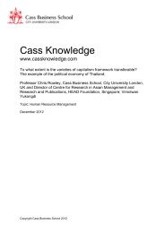
Chart 1 shows that <strong>the</strong> number <strong>of</strong> shares purchased in period 5 <strong>of</strong> our simulations by VA <strong>and</strong><br />
DCA are highly correlated, but <strong>the</strong> range <strong>of</strong> variation is much larger for VA. This illustrates its<br />
greater tendency to average down, <strong>and</strong> hence to achieve a lower average cost.<br />
DCA shares purchased<br />
60<br />
55<br />
50<br />
45<br />
40<br />
35<br />
30<br />
25<br />
Chart 1: Total Number Of Shares Purchased<br />
Under DCA <strong>and</strong> VA<br />
25 30 35 40 45 50 55 60<br />
VA shares purchased<br />
Table 4 gives a different example which shows that <strong>the</strong>se effects also apply when prices rise. In<br />
period two prices have risen to $1.10, so purchases made in period one now look cheap. The<br />
best way to achieve a low average purchase cost is <strong>the</strong>n to buy very few shares at this higher<br />
price. ESA does badly here, buying ano<strong>the</strong>r 100 shares, <strong>and</strong> thus “doubling up” <strong>the</strong> average<br />
purchase price to $1.05. DCA buys 91 shares, <strong>and</strong> VA buys only 82 as <strong>the</strong> capital gain on its<br />
initial investment helps to achieve its target portfolio <strong>value</strong> without needing fur<strong>the</strong>r investment.<br />
Thus VA again achieves <strong>the</strong> lowest average purchase price, <strong>the</strong>n DCA, with ESA highest again.<br />
But none <strong>of</strong> this alters expected pr<strong>of</strong>its.<br />
Table 4 Equal Share Amounts (ESA) Dollar Cost Averaging (DCA) Value Averaging (VA)<br />
Period Price<br />
Shares<br />
bought<br />
Invest-<br />
ment<br />
($)<br />
Portfolio<br />
($)<br />
Shares<br />
bought<br />
7<br />
Invest-<br />
ment<br />
($)<br />
Portfolio<br />
($)<br />
Shares<br />
bought<br />
Invest-<br />
ment<br />
($)<br />
1 1.00 100 100 100 100 100 100 100 100 100<br />
2 1.10 100 110 231 91 100 220 82 90 200<br />
3 1.20 100 120 396 83 100 360 68 82 300<br />
Total 300 330 274 300 250 272<br />
Average cost: 1.10 1.094 1.087<br />
Portfolio<br />
($)
Difference in average cost ($)<br />
0.00<br />
-0.01<br />
-0.02<br />
-0.03<br />
-0.04<br />
-0.05<br />
-0.06<br />
-0.07<br />
Chart 2: Comparative Average Purchase Cost Achieved<br />
By Different Strategies<br />
DCA avg. cost - ESA avg. cost<br />
VA avg. cost - ESA avg. cost<br />
8 9 10 11 12<br />
Terminal share price ($)<br />
The simulations confirm <strong>the</strong>se points. Chart 2 compares <strong>the</strong> average costs achieved by <strong>the</strong>se<br />
three strategies. We can see that:<br />
(i) DCA <strong>and</strong> VA always achieve lower average purchase costs than ESA (<strong>and</strong> VA<br />
always achieves a greater cost reduction than DCA because <strong>of</strong> its more<br />
aggressive response to share price movements).<br />
(ii) The difference is largest where <strong>the</strong> terminal price PT has moved a long way from<br />
<strong>the</strong> starting <strong>value</strong>. Volatile share prices allow DCA <strong>and</strong> VA greater scope to<br />
benefit from buying more shares at low prices. Conversely, if prices do not vary<br />
at all, <strong>the</strong> three strategies will be identical.<br />
Proponents <strong>of</strong> DCA almost invariably assume that a strategy which buys at lower average cost<br />
must lead to higher pr<strong>of</strong>its. The continued popularity <strong>of</strong> DCA (in spite <strong>of</strong> academic studies which<br />
show it to be a sub-optimal strategy) suggests that investors generally find this argument highly<br />
persuasive.<br />
All else equal, lower average costs must indeed lead to higher pr<strong>of</strong>its, but all else is not equal.<br />
This can be shown by comparing <strong>the</strong> total amount invested by <strong>the</strong> different strategies with <strong>the</strong><br />
share price at <strong>the</strong> end <strong>of</strong> <strong>the</strong> simulation (Chart 3). The ESA strategy naturally invests more in<br />
simulations where prices end up falling, <strong>and</strong> less when <strong>the</strong>y are falling. By contrast, DCA invests<br />
a fixed total dollar amount ($2000 for <strong>the</strong>se simulations). The fact that DCA invests at a lower<br />
average cost is balanced by <strong>the</strong> fact that it tends to invest a smaller amount in periods <strong>of</strong> rising<br />
prices <strong>and</strong> more in periods <strong>of</strong> falling prices. These factors tend to cancel out: as we saw earlier,<br />
<strong>the</strong> expected pr<strong>of</strong>its <strong>of</strong> <strong>the</strong> two strategies are identical.<br />
This <strong>bias</strong> is even more pronounced for VA, which tends to invest less during periods <strong>of</strong> rising<br />
prices (since capital gains help achieve <strong>the</strong> investor’s desired portfolio <strong>value</strong> without <strong>the</strong> need for<br />
substantial additional investment). Thus a VA strategy tends to invest far less than ESA during<br />
periods <strong>of</strong> rising prices <strong>and</strong> far more in periods <strong>of</strong> falling prices. This <strong>of</strong>fsets <strong>the</strong> fact that VA<br />
achieves a lower average cost. Once again, expected pr<strong>of</strong>its are identical for <strong>the</strong> two strategies.<br />
8
Total amount invested ($)<br />
2200<br />
2100<br />
2000<br />
1900<br />
1800<br />
Chart 3: Total Amount Invested By Each Strategy<br />
ESA<br />
DCA<br />
VA<br />
8.0 9.0 10.0 11.0 12.0<br />
Terminal share price ($)<br />
Ingersoll et al. (2007) show that cynical investment managers can manipulate conventional<br />
performance measures (including <strong>the</strong> Sharpe ratio, Jensen’s alpha etc.). The ‘gaming’ <strong>of</strong> <strong>the</strong>se<br />
performance measures is achieved by reducing risk exposure following a good performance <strong>and</strong><br />
increasing exposure after a poor performance. This strategy could be characterized as applying<br />
an element <strong>of</strong> “quit while you are ahead, gamble more when you are behind”. DCA <strong>and</strong> VA in<br />
effect use this strategy automatically, since by construction <strong>the</strong>y invest more following price falls<br />
<strong>and</strong> less after price rises. This allows <strong>the</strong>m to achieve low average purchase costs without<br />
achieving any increase in pr<strong>of</strong>itability. The following section shows that <strong>the</strong> same <strong>bias</strong> applies to<br />
<strong>the</strong> IRRs achieved by <strong>the</strong>se strategies.<br />
5. The Bias In IRRs<br />
The section above showed that DCA <strong>and</strong> VA achieve lower average costs, but <strong>the</strong> same<br />
expected pr<strong>of</strong>its as ESA. However, VA is a more complex strategy than DCA, with varying<br />
cashflows, so proponents <strong>of</strong> VA focus instead on <strong>the</strong> fact that it tends to generate a higher<br />
internal rate <strong>of</strong> return than ei<strong>the</strong>r ESA or DCA. Our simulations confirm (Table 3 <strong>and</strong> Chart 4) that<br />
IRRs are generally higher for VA than for DCA, with both strategies giving higher average IRRs<br />
than ESA 3 . It might appear intuitive that a higher IRR will imply higher expected pr<strong>of</strong>its, but in this<br />
section we show that <strong>the</strong>se IRRs are misleading, since <strong>the</strong> same <strong>bias</strong> is at work as we found for<br />
average costs.<br />
3 Marshall (2000) calculates which strategy gives <strong>the</strong> highest IRR for each simulated path. In 73.5% <strong>of</strong> cases<br />
VA was best, with DCA best in only 3.9% <strong>of</strong> cases. Chart 4 helps explain this: where <strong>the</strong> simulated price path<br />
tends to mean-revert, <strong>the</strong> aggressive VA strategy generally gives <strong>the</strong> highest IRR. Where prices make<br />
sustained movements, strategies with no dynamic component fare better (ESA here, or Marshall’s r<strong>and</strong>om<br />
investing strategy). The less aggressive DCA strategy is almost always outperformed by one <strong>of</strong> <strong>the</strong> o<strong>the</strong>r two<br />
strategies, but frequently comes in second place, consistent with <strong>the</strong> results in Table 3 showing that it<br />
records a higher average IRR than ESA.<br />
9
IRR differential<br />
Chart 4: Comparative IRRs Achieved By Different<br />
Strategies<br />
0.15%<br />
0.10%<br />
0.05%<br />
0.00%<br />
-0.05%<br />
8.0 9.0 10.0 11.0 12.0<br />
Terminal share price ($)<br />
10<br />
VA IRR - ESA IRR<br />
DCA IRR - ESA IRR<br />
We can illustrate this by comparing <strong>the</strong> investments made by each strategy in <strong>the</strong> second period.<br />
Again we initially consider <strong>the</strong> scenario <strong>of</strong> falling prices shown in Table 1. By period 2 each <strong>of</strong> <strong>the</strong><br />
strategies has made a $10 loss on <strong>the</strong> $100 invested in <strong>the</strong> first period <strong>and</strong> <strong>the</strong> assumption <strong>of</strong> a<br />
driftless r<strong>and</strong>om walk means that this loss must be expected to persist, leading to a negative<br />
overall expected IRR.<br />
However, <strong>the</strong> ex ante expected IRR <strong>of</strong> any sum we invest in period 2, taken in isolation, is zero.<br />
The overall IRR on our combined investment in periods 1 <strong>and</strong> 2 will depend on <strong>the</strong> IRRs <strong>of</strong> <strong>the</strong>se<br />
investments taken separately, <strong>and</strong> <strong>the</strong> relative amounts invested in each <strong>of</strong> <strong>the</strong>se periods. This<br />
relationship is polynomial, but <strong>the</strong> direction <strong>of</strong> <strong>the</strong> relationship is intuitive: if prices have fallen in<br />
period 2, <strong>the</strong> expected IRR on <strong>the</strong> amount invested in period 1 (IRR1) is now negative, but <strong>the</strong><br />
expected IRR on <strong>the</strong> amount that we are about to invest in period 2 (IRR2) is still zero. The more<br />
that we invest in <strong>the</strong> second period, <strong>the</strong> more <strong>the</strong> expected IRR on <strong>the</strong> two investments combined<br />
(IRRc) is likely to move away from IRR1 <strong>and</strong> towards IRR2 (ie. zero) 4 . Thus if our objective is to<br />
maximize IRRc, our best response in period 2 to <strong>the</strong> loss made already would be to dilute <strong>the</strong><br />
negative IRR1 with a large new investment which carries a zero expected IRR.<br />
As we have seen, this is exactly what DCA does by automatically investing more following a fall<br />
in prices. VA does <strong>the</strong> same, but more aggressively. This process is very similar to <strong>the</strong> doubling<br />
down we saw in <strong>the</strong> previous section, <strong>the</strong> only difference being that <strong>the</strong> more complex arithmetic<br />
<strong>of</strong> <strong>the</strong> IRR means that this is no longer a simple <strong>averaging</strong>, but a more complex dilution effect.<br />
Conversely, if prices rise after our initial investment, <strong>the</strong>n our expected IRR1 is positive, whilst our<br />
expected IRR2 is still zero. The best strategy for maximizing our expected IRRc would thus be to<br />
invest relatively little in <strong>the</strong> second period, to avoid diluting <strong>the</strong> positive expected IRR1 with <strong>the</strong><br />
zero expected IRR2.<br />
4 The polynomial arithmetic <strong>of</strong> IRRs means that <strong>the</strong>re may be exceptions to this. Indeed, VA can entail <strong>the</strong><br />
return <strong>of</strong> cash to investors in some periods (where a large price rise results in a capital gain that is greater<br />
than <strong>the</strong> target increase in portfolio <strong>value</strong>). Thus <strong>the</strong>re may be multiple swings from positive to negative<br />
cashflow, so we cannot rule out multiple roots in our IRR calculation. However, as long as it is generally true<br />
that <strong>the</strong> aggregate IRR is <strong>bias</strong>ed towards zero by investing larger amounts in <strong>the</strong> current period, <strong>the</strong>n <strong>the</strong>re<br />
will be a <strong>bias</strong> in <strong>the</strong> average IRR. Our simulations confirm that this is indeed <strong>the</strong> case.
Phalippou (2008) notes that <strong>the</strong> IRRs recorded by private equity managers can be manipulated<br />
by adjusting <strong>the</strong> cashflows involved: returning cash to investors rapidly for projects with high IRRs<br />
<strong>and</strong> extending <strong>the</strong> exposure <strong>of</strong> poorly-performing projects. This is similar to <strong>the</strong> mechanism noted<br />
by Ingersoll et al. (2007) for <strong>bias</strong>ing o<strong>the</strong>r performance measures. The <strong>bias</strong> in each case is<br />
achieved by reducing exposure following a good outturn <strong>and</strong> increasing exposure following a bad<br />
outturn. By doing this automatically, DCA <strong>and</strong> VA achieve IRRs which are better than ESA, whilst<br />
<strong>the</strong>ir ex ante expected pr<strong>of</strong>its remain zero.<br />
Difference in pr<strong>of</strong>it ($)<br />
6<br />
4<br />
2<br />
0<br />
-2<br />
-4<br />
-6<br />
-8<br />
-10<br />
-12<br />
-14<br />
Chart 5: Comparative Pr<strong>of</strong>its<br />
DCA Pr<strong>of</strong>it - ESA Pr<strong>of</strong>it<br />
VA Pr<strong>of</strong>it - ESA Pr<strong>of</strong>it<br />
8.0 9.0 10.0 11.0 12.0<br />
Terminal share price ($)<br />
Chart 5 shows <strong>the</strong> increase or decrease in pr<strong>of</strong>its generated by each <strong>of</strong> <strong>the</strong> formula trading<br />
strategies compared to a static ESA strategy. As we saw in Table 3, <strong>the</strong> differential averages<br />
zero, but <strong>the</strong> formula trading strategies outperform when <strong>the</strong> share price ends up relatively close<br />
to its starting <strong>value</strong> ($10). These strategies buy more shares at relatively low prices, <strong>and</strong> when<br />
prices mean-revert this lower average cost does translate into higher pr<strong>of</strong>its (with none <strong>of</strong> <strong>the</strong><br />
<strong>of</strong>fsetting downside illustrated in Chart 3). This advantage is larger for VA, with its more<br />
aggressive response to changing share prices, than it is for DCA. Conversely, DCA <strong>and</strong> VA do<br />
poorly in sustained price trends, since <strong>the</strong>y purchase more shares than ESA in downtrends <strong>and</strong><br />
fewer shares than ESA in uptrends.<br />
Thus VA can be pr<strong>of</strong>itable where investors correctly anticipate mean-reversion (implying that<br />
markets are to some extent forecastable). But this is a dramatic contrast to <strong>the</strong> claim made by<br />
proponents <strong>of</strong> VA that <strong>the</strong> strategy increases expected returns in any market, even when<br />
investors have no ability to forecast returns. Fur<strong>the</strong>rmore, even where <strong>the</strong>re is an element <strong>of</strong><br />
mean reversion, o<strong>the</strong>r dynamic strategies (e.g. based on calibrated filter rules) are likely to be<br />
more efficient mechanisms for pr<strong>of</strong>iting from such forecastable price movements.<br />
6. Risk And Cashflow<br />
We have established that VA, like DCA, cannot expect to generate excess pr<strong>of</strong>its in markets<br />
where price movements cannot be forecast. We now consider briefly <strong>the</strong> effects that VA has on<br />
cashflow management <strong>and</strong> risk levels.<br />
11
DCA generates perfectly stable cashflows by construction, with a fixed dollar amount invested<br />
each period. Thus even though <strong>the</strong> strategy is mean-variance inefficient, it can claim <strong>the</strong><br />
incidental benefit <strong>of</strong> encouraging regular savings. Just as for DCA, <strong>the</strong> case for VA is based on a<br />
misleading claim <strong>of</strong> superior returns, but VA comes with <strong>the</strong> added drawback <strong>of</strong> highly uncertain<br />
investor cashflows, since <strong>the</strong> amount which must be invested each period depends on <strong>the</strong> most<br />
recent movements in <strong>the</strong> market price (VA can even imply an unexpected return <strong>of</strong> cash to <strong>the</strong><br />
investor following a large price rise). Indeed, <strong>the</strong>se cashflows are likely to become increasingly<br />
volatile over time as <strong>the</strong> existing portfolio increases in size relative to <strong>the</strong> target increase in <strong>value</strong><br />
each period. Edelson (1991) envisages investors holding a ‘side fund’ containing liquid assets<br />
sufficient to meet <strong>the</strong>se needs.<br />
As for risk, Table 2 shows that <strong>the</strong> pr<strong>of</strong>its recorded by <strong>the</strong> gradual investment strategies (ESA,<br />
DCA <strong>and</strong> VA) have almost identical st<strong>and</strong>ard deviations, but pr<strong>of</strong>its on <strong>the</strong> lump-sum strategy are<br />
more volatile. However, it would be a mistake to conclude that this is an advantage to using<br />
gradualist strategies. DCA, VA <strong>and</strong> ESA all keep a large proportion <strong>of</strong> <strong>the</strong> available funds in cash,<br />
<strong>and</strong> so will naturally record a lower level <strong>of</strong> volatility. By contrast, <strong>the</strong> lump-sum strategy is always<br />
fully exposed. In our example <strong>of</strong> a r<strong>and</strong>om walk with zero drift, this cash allocation is not<br />
penalized, but if instead long-term expected returns on <strong>the</strong> chosen asset are higher than <strong>the</strong> risk<br />
free rate, <strong>the</strong>n delayed investment will come at <strong>the</strong> cost <strong>of</strong> lower expected returns.<br />
In normal circumstances we might turn to performance measures such as <strong>the</strong> Sharpe ratio to<br />
assess whe<strong>the</strong>r <strong>the</strong> resulting trade-<strong>of</strong>f between lower risk <strong>and</strong> lower expected return is<br />
worthwhile, but such measures are systematically <strong>bias</strong>ed here. However, <strong>the</strong> intuition <strong>of</strong> <strong>the</strong> point<br />
made by Rozeff (1994) applies: DCA is mean-variance inefficient because it gives insufficient<br />
time diversification, concentrating <strong>the</strong> risk into later periods. We should expect VA to be similarly<br />
inefficient compared to lump-sum investment.<br />
7. Conclusion<br />
The small amount <strong>of</strong> previous academic work on VA concludes that it generates higher expected<br />
pr<strong>of</strong>its than alternative strategies even when price movements are unforecastable. This paper<br />
shows that DCA <strong>and</strong> VA do indeed achieve lower average costs <strong>and</strong> higher IRRs than alternative<br />
strategies, but <strong>the</strong>y do not give higher expected pr<strong>of</strong>its. Instead an “<strong>averaging</strong> down” effect<br />
systematically <strong>bias</strong>es <strong>the</strong> IRR up <strong>and</strong> <strong>the</strong> average purchase cost down.<br />
We first noted that where price movements are unforecastable no formula investment strategy<br />
can expect to generate excess returns. The expected excess return is zero for each period, so<br />
strategies which alter <strong>the</strong> amount invested in each period cannot change this expectation. We<br />
<strong>the</strong>n presented simulations which confirmed that VA achieves a higher expected IRR <strong>and</strong> lower<br />
average purchase cost than alternative strategies, but it does not generate higher pr<strong>of</strong>its.<br />
Previous studies have shown that investment managers can <strong>bias</strong> IRRs <strong>and</strong> Sharpe ratios by<br />
manipulating future risk exposures in <strong>the</strong> light <strong>of</strong> <strong>the</strong> returns already achieved. DCA <strong>and</strong> VA<br />
automatically manipulate <strong>the</strong>ir exposures in this way, by buying more after a fall in prices, <strong>and</strong><br />
less after a price rise. It is only for this reason that <strong>the</strong>y appear to outperform o<strong>the</strong>r strategies.<br />
The same <strong>bias</strong> will apply to a wide class <strong>of</strong> investment strategies where <strong>the</strong> amount invested in<br />
each period is negatively correlated with <strong>the</strong> return made to date.<br />
In conclusion, VA has little to recommend it. Contrary to <strong>the</strong> claims made by previous studies it<br />
does not improve expected pr<strong>of</strong>its unless <strong>the</strong>re is systematic mean reversion. Moreover, it<br />
causes unpredictable cashflows <strong>and</strong> requires a large holding <strong>of</strong> liquid assets which is likely to<br />
result in portfolios which are mean/variance inefficient.<br />
12
References<br />
Constantinides, G.M. 1979. “A note On The Suboptimality Of Dollar-Cost Averaging As An<br />
Investment Policy.” Journal <strong>of</strong> Financial <strong>and</strong> Quantitative Analysis, vol.14, no. 2 (June): 443-450.<br />
Edleson, M.E. 1991 “Value Averaging: The Safe <strong>and</strong> Easy Strategy for Higher Investment<br />
Returns.” Wiley Investment Classics, revised edition 2006.<br />
Edleson, M.E. 1988 “Value Averaging: A New Approach To Accumulation.” American Association<br />
<strong>of</strong> Individual Investors Journal vol. X, no. 7 (August 1988)<br />
Hayley, S. 2009. “Explaining <strong>the</strong> Riddle <strong>of</strong> Dollar Cost Averaging”, <strong>Cass</strong> Business School working<br />
paper.<br />
Ingersoll, J; Spiegel, M; Goetzmann, W <strong>and</strong> Welch, I. (2007) "Portfolio Performance Manipulation<br />
<strong>and</strong> Manipulation-pro<strong>of</strong> Performance Measures," Review <strong>of</strong> Financial Studies 20-5, September<br />
2007, 1503-1546.<br />
Knight, J.R. <strong>and</strong> M<strong>and</strong>ell, L. 1992/93. “Nobody Gains From Dollar Cost Averaging: Analytical,<br />
Numerical And Empirical Results.” Financial Services Review, vol. 2, issue 1: 51-61.<br />
Marshall, P.S. 2000. “A Statistical Comparison Of Value Averaging Vs. Dollar Cost Averaging<br />
And R<strong>and</strong>om Investment Techniques.” Journal <strong>of</strong> Financial <strong>and</strong> Strategic Decisions, vol. 13, no.<br />
1 (Spring) 87-99.<br />
Marshall, P.S. 2006 “A multi-market, historical comparison <strong>of</strong> <strong>the</strong> investment returns <strong>of</strong> <strong>value</strong><br />
<strong>averaging</strong>, dollar cost <strong>averaging</strong> <strong>and</strong> r<strong>and</strong>om investment techniques.” Academy <strong>of</strong> Accounting<br />
<strong>and</strong> Financial Studies Journal, Sept 2006.<br />
Milevsky, M. A. <strong>and</strong> Posner, S. E. 2003 "A Continuous-Time Re-examination <strong>of</strong> <strong>the</strong> Inefficiency <strong>of</strong><br />
Dollar-Cost Averaging" International Journal <strong>of</strong> Theoretical & Applied Finance, Mar 2003, Vol. 6<br />
Issue 2.<br />
Phalippou, L. 2008 “The Hazards <strong>of</strong> Using IRR to Measure Performance: The Case <strong>of</strong> Private<br />
Equity”. Journal <strong>of</strong> Performance Measurement, Fall issue.<br />
Rozeff, M.S. 1994. “Lump-sum Investing Versus Dollar-Averaging.” Journal <strong>of</strong> Portfolio<br />
Management, vol. 20, issue 2 (winter): 45-50.<br />
Thorley, S.R. 1994. “The fallacy <strong>of</strong> Dollar Cost Averaging.” Financial Practice <strong>and</strong> Education, vol.<br />
4, no. 2 (Fall/Winter): 138-143.<br />
Williams, R.E. <strong>and</strong> Bacon, P.W. 1993. “Lump-sum Beats Dollar Cost Averaging.” Journal <strong>of</strong><br />
Financial Planning, vol. 6, no.2 (April): 64–67.<br />
13