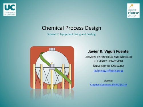
Chemical Process Design

Chemical
Process
Design
Subject
7.
Equipment
Sizing
and
Cos8ng
Javier
R.
Viguri
Fuente
CHEMICAL
ENGINEERING
AND
INORGANIC
CHEMISTRY
DEPARTMENT
UNIVERSITY
OF
CANTABRIA
javier.viguri@unican.es
License:
Crea8ve
Commons
BY‐NC‐SA
3.0

INDEX
1.- Introduction
• Categories of total capital cost estimates
• Cost estimation method of Guthrie
2.- Short cuts for equipment sizing procedures
• Vessel (flash drums, storage tanks, decanters and some reactors)
• Reactors
• Heat transfer equipment (heat exchangers, furnaces and direct fired heaters)
• Distillation columns
• Absorbers columns
• Compressors (or turbines)
• Pumps
• Refrigeration
3.- Cost estimation of equipment
• Base costs for equipment units
• Guthrie´s modular method
4.- Further Reading and References
2

1.- INTRODUCTION
Process Alternatives Synthesis (candidate flowsheet)
Analysis (Preliminary mass and energy balances)
SIZING (Sizes and capacities)
COST ESTIMATION (Capital and operation)
Economic Analysis (economic criteria)
SIZING
Calculation of all physical attributes that allow a unique costing of this unit
- Capacity, Height - Pressure rating
-Cross sectional area – Materials of construction
Short-cut, approximate calculations (correlations) Quick obtaining of
sizing parameters Order of magnitude estimated parameters
COST
Total Capital Investment or Capital Cost: Function of the process
equipment The sized equipment will be costed
* Approximate methods to estimate costs
Manufacturing Cost: Function of process equipment and utility charges
3

Categories of total capital cost estimates
based on accuracy of the estimate
ESTIMATE BASED ON Error (%) Obtention USED TO
ORDER OF
MAGNITUDE
(Ratio estimate)
STUDY
PRELIMINARY
DEFINITIVE
Method of Hill, 1956. Production rate
and PFD with compressors, reactors
and separation equipments. Based
on similar plants.
Overall Factor Method of Lang, 1947.
Mass & energy balance and
equipment sizing.
Individual Factors Method of Guthrie,
1969, 1974. Mass & energy balance,
equipment sizing, construction
materials and P&ID. Enough data to
budget estimation.
Full data but before drawings and
specifications.
40 - 50 Very fast Profitability
analysis
25 - 40 Fast
15 - 25 Medium
10 -15 Slow
DETAILED Detailed Engineering 5 -10 Very slow
Preliminary
design
Budget
approval
Construction
control
Turnkey
contract
4

Cost Estimation Method of Guthrie
• Equipment purchase cost: Graphs and/or equations.
Based on a power law expression: Williams Law C = BC =Co (S/So) α
Economy of Scale (incremental cost C, decrease with larger capacities S)
Based on a polynomial expression BC = exp {A 0 + A 1 [ln (S)] + A 2 [ln (S) ] 2 +…}
• Installation: Module Factor, MF, affected by BC, taking into account
labor, piping instruments, accessories, etc.
Typical Value of MF=2.95 equipment cost is almost 3 times the BC.
Installation = (BC)(MF)-BC = BC(MF-1)
• For special materials, high pressures and special designs abroad base
capacities and costs (Co, So), the Materials and Pressure correction
Factors, MPF, are defined.
Uninstalled Cost = (BC)(MPF) Total Installed Cost = BC (MPF+MF-1)
• To update cost from mid-1968, an Update Factor, UF to account for
inflation is apply.
UF: Present Cost Index/Base Cost index
Updated bare module cost: BMC = UF(BC) (MPF+MF-1)
5

Materials and Pressure correction Factors: MPF
Empirical factors that modified BC and evaluate particular instances of
equipment beyond a basic configuration: Uninstalled Cost = (BC x MPF)
MPF = Φ Φ (Fd, Fm, Fp, Fo, Ft)
Fd: Design variation Fm: Construction material variation
Fp: Pressure variation Fo: Operating Limits ( Φ Φ of T, P)
Ft: Mechanical refrigeration factor Φ Φ Φ ( (T ( evaporator)
EQUIPMENT MPF
Pressure Vessels Fm . Fp
Heat Exchangers Fm (Fp + Fd)
Furnaces, direct fired heaters, Tray stacks Fm + Fp + Fd
Centrifugal pumps Fm . Fo
Compressors Fd
Equipment Sizing Procedures
Need C and MPF required the flowsheet mass and energy balance
(Flow, T, P, Q)
6

An example of Cost Estimation
Equipment
purchase price
Design Factor
Fd
Cp
Total Cost =
UF
Material Factor
Fm
Pressure
Factor
Fp
Factor Base
Modular
Fbm
7

2.- EQUIPMENT SIZING PROCEDURES
Q, P
maintenance
∆ Heat
contents
∆
Composition
Q, P
streams
setting
Vessels
V
Heat transfer equipment: Heat exchangers
Furnaces and Direct Fired Heaters
Refrigeration
Reactors
Columns, distillation and Absorption
Pumps, Compressors and Turbines
Short-cut calculations
for the main
equipment sizing
5
P1
H1IN
D1
CT
C1
HX1
C1
8

SHORTCUTS for VESSEL SIZING (Flash drums, storage tanks, decanters and
some reactors)
1) Select the V for liquid holdup; τ= 5 min + equal vapor volume
V=(F L /ρ L * τ)*2
2) Select L=4D
•Materials of Construction appropriate to use with the Guthrie´s factors
and pressure (P rated =1.5 P actual )
• Basic Configuration for pressure vessels
F
V=πD 2 /4*L D=(V/π) 1/3 ; If D ≤1.2 m Vertical, else Horizontal
V
FV
- Carbon steel vessel with 50 psig design P and average nozzles and manways
- Vertical construction includes shell and two heads, the skirt, base rings and lugs, and
possible tray supports.
- Horizontal construction includes shell, two heads and two saddles
MPF = Fm . Fp; Fm depending shell material configuration (clad or solid)
FL
V
V2
9

High Temperature Service
Tmax ( o F) Steel
950 Carbon steel (CS)
1150 502 stainless steels (SS)
1300 410 SS; 330 SS
1500 304,321,347,316 SS.
Hastelloy C, X Inconel
Materials of Construction for Pressure Vessels
2000 446 SS, Cast stainless, HC
Low Temperature Service
Tmin ( o F) Steel
-50 Carbon steel (CS)
-75 Nickel steel (A203)
-320 Nickel steel (A353)
-425 302,304,310,347 (SS)
Guthrie Material and pressure factors for pressure vessels: MPF = Fm Fp
Shell Material Clad, Fm Solid, Fm
Carbon Steel (CS) 1.00 1.00
Stainless 316 (SS) 2.25 3.67
Monel (Ni:Cr/2:1 alloy) 3.89 6.34
Titanium 4.23 7.89
Vessel Pressure (psig)
Up to 50 100 200 300 400 500 900 1000
Fp 1.00 1.05 1.15 1.20 1.35 1.45 2.30 2.50
10

SHORT CUT for REACTORS SIZING
First step of the preliminary design Not kinetic model available.
Mass Balance based on Product distribution High influence in final cost
Assumptions: Reactor equivalent to laboratory reactor, adiabatic reactors
are isotherm at average T.
Assume space velocity (S in h -1 )
S = (1/τ) = µ µ /ρ /ρ Vcat ; V = Vcat / 1- ε
µ = Flow rate; ρ= molar density; V cat= Volume of catalyst; ε= Void fraction of catalyst (e.g. ε=0.5)
5
R
1
R2
11

HEAT TRANSFER EQUIPMENT SIZING
Heat exchanger types used in chemical process
By function
- Refrigerants (air or water) - Condensers (v, v+l l) - Reboilers, vaporizers (lv) - Exchangers in general
By constructive shape
- Double pipe exchanger: the simplest one - Shell and tube exchangers: used for all applications
- Plate and frame exchangers - Air cooled: used for coolers and condensers
- Direct contact: used for cooling and quenching - Jacketed vessels, agitated vessels and internal coils
- Fired heaters: Furnaces and boilers
Shell and tube countercurrent exchanger, steady state
Q = U A ∆T lm
Q: From the energy balance
U: Estimation of heat transfer coefficient. Depending on configuration and media used
in the Shell and Tube side: L-L, Condensing vapor-L, Gas-L, Vaporizers). (Perry's
Handbook, 2008; www.tema.org).
A: Area
∆T lm : Logarithmic Mean ∆T = (T1-t2)-(T2-t1)/ln (T1-t2/T2-t1)
- If phase changes Approximation of 2 heat exchangers (A=A1+A2)
- Maximum area A ≤ 1000 m 2 , else Parallel HX
MPF: Fm (Fp + Fd)
H1
C11
T1 T2
t2
EX1
t1
H11
C1
12

Heat exchanger: Countercurrent, steady state HX1
Guthrie Material and pressure factors for Heat Exchangers: MPF: Fm (Fp + Fd)
Design Type Fd Vessel Pressure (psig)
Kettle Reboiler 1.35
Floating Head 1.00 Up to 150 300 400 800 1000
U Tube 0.85 Fp 0.00 0.10 0.25 0.52 0.55
Fixed tube sheet 0.80
Shell/Tube Materials, Fm
Surface Area (ft 2 ) CS/ CS/ CS/ SS/ CS/ Monel CS/ Ti/
CS Brass SS SS Monel Monel Ti Ti
Up to 100 1.00 1.05 1.54 2.50 2.00 3.20 4.10 10.28
100 to 500 1.00 1.10 1.78 3.10 2.30 3.50 5.20 10.60
500 to 1000 1.00 1.15 2.25 3.26 2.50 3.65 6.15 10.75
1000 to 5000 1.00 1.30 2.81 3.75 3.10 4.25 8.95 13.05
13

FURNACES and DIRECT FIRED HEATERS (boilers,reboilers, pyrolysis, reformers)
Q = Absorbed duty from heat balance
• Radiant section (q r =37.6 kW/m 2 heat flux) + Convection section (q c =12.5 kW/m 2
heat flux). Equal heat transmission (kW) A rad =0.5 x kW/q r ; A conv =0.5 x kW/q c
• Basic configuration for furnaces is given by a process heater with a box or Aframe
construction, carbon steel tubes, and a 500 psig design P. This includes
complete field erection.
• Direct fired heaters is given by a process heater with cylindrical construction,
carbon steel tubes, and a 500 psig design.
Guthrie MPF for Furnaces: MPF= Fm+Fp+Fd
Design Type Fd
Process Heater 1.00
Pyrolisis 1.10
Reformer 1.35
Vessel Pressure (psig)
Up to 500 1000 1500 2000 2500 3000
Fp 0.00 0.10 0.15 0.25 0.40 0.60
Radiant Tube Material, Fm
Carbon Steel 0.00
Chrome/Moly 0.35
Stainless Steel 0.75
Guthrie MPF for Direct Fired Heaters
MPF: Fm + Fp + Fd
Design Type Fd
Cylindrical 1.00
Dowtherm 1.33
Vessel Pressure (psig)
Up to 500 1000 1500
Fp 0.00 0.15 0.20
Radiant Tube Material, Fm
Carbon Steel 0.00
Chrome/Moly 0.45
Stainless Steel 0.50
14

HEAT EXCHANGERS
15

SHORT CUT for DISTILLATION COLUMS SIZING
Fenske's equation applies to any two components lk and hk at infinite reflux and is
defined by N min , where αij is the geometric mean of the α's at the T of the feed,
distillate and the bottoms.
( α )
lk / hk
R min is given by Underwood with two equations that must be solved, where q is
the liquid fraction in the feed..
Gilliland used an empirical correlation to
calculate the final number of stage N from
the values calculated through the Fenske
and Underwood equations (N min , R, R min ).
The procedure use a diagram; one enters
with the abscissa value known, and read
the ordinate of the corresponding point on
the Gilliland curve. The only unknown of
the ordinate is the number of stage N.
⎛ x Dlk / x ⎞ Blk
log ⎜⎜
x Dhk / x ⎟⎟
Bhk
N min =
⎝
⎠
α lk / hk = D lk / hk F lk / hkα
log
( ) 3 / 1
α α
B lk / hk
16

SHORT CUT for DISTILLATION COLUMS SIZING
Simple and direct correlation for (nearly) ideal systems (Westerberg, 1978)
• Determine α lk/hk ; β lk = ξ lk ; β hk = 1- ξ hk
• Calculate tray number Ni and reflux ratio Ri from correlations (i= lk, hk):
Ni = 12.3 / (α lk/hk -1) 2/3 . (1- β i ) 1/6 Ri = 1.38 / (α lk/hk -1) 0.9 . (1- β i ) 0.1
- Theoretical nº of trays N T = 0.8 max[Ni] + 0.2 min[Ni]; R= 0.8 max[Ri] + 0.2 min[Ri]
- Actual nº of trays N = N T /0.8
- For H consider 0.6 m spacing (H=0.6 N); Maximum H=60 m else, 2 columns
* Calculate column diameter, D, by internal flowrates and taking into account
the vapor fraction of F. Internal flowrates used to sizing condenser, reboiler
Design column at 80% of linear flooding velocity
π D
A =
4
2
⎡ V ⎤
= ⎢
⎥
⎢⎣
0.
8U
f ε ρG
⎥⎦
If D> 3m Parallel columns
* Calculate heat duties for reboiler and condenser
n
n
k k k V
k
∑(
µ
D + µ L ) ∆H
vap = µ dk H
Q ∆
cond = HV
− H L =
∑
k=
1
D k = 1
* Costing vessel and stack trays (24” spacing)
vap
U
f
reb
= C
sb
⎡ ρ ⎤
L − ρG
⎢ ⎥
⎣ ρG
⎦
Q = V ∆H
k
vap
0.
5
⎛ 20 ⎞
⎜ ⎟⎠
⎝ σ
0.
2
17

DISTILLATION COLUMNS
Guthrie MPF for Tray
Stacks
MPF: Fm + Fs + Ft
Tray Type Ft
Grid 0.0
Plate 0.0
Sieve 0.0
Valve o trough 0.4
Bubble Cap 1.8
Koch Kascade 3.9
Tray Spacing, Fs
(inch) 24” 18” 12”
Fs 1.0 1.4 2.2
Tray Material, Fm
Carbon Steel 0.0
Stainless Steel 1.7
Monel 8.9
D1
D2
18

DISTILLATION COLUMNS
19

SHORT CUT for ABSORBERS COLUMS SIZING
Sizing similar to the distillation columns
N T Kremser equation
n n n n
⎡l
+ ( r − A ) v ⎤
0
E N+
1
n
N = ln⎢
/ ln( A )
n n
n n
E
l A ( 1 r ) v
⎥
⎣ − −
0 E
N+
1 ⎦
• Assumption: v-l equilibrium but actually there is mass transfer phenomena (e.g.
simulation of CO 2 - MEA absorption) 20% efficiency in nº trays N = N T /0.2
• Calculate H and D for costing vessel and stack trays (24” spacing)
E1
20

SHORT CUT for COMPRESSORS (or TURBINES) SIZING
Compressor
P1, T1 P2, T2
µ
Centrifugal compressors are the most common compressors (High capacities, low
compression ratios –r-) vs. Reciprocating compressors (Low capacities, high r)
Assumptions: Ideal behavior, isentropic and adiabatic
Drivers
1) Electric motors driving compressor; η M =0.9; η C =0.8 (compressor)
Brake horsepower W b = W/η M η C = 1.39 W
2) Turbine diving compressor (e.g.IGCC where need decrease P); η T =0.8; W b =1.562 W
Max. Horsepower compressor = 10.000 hp = 7.5 MW
Max Compression ratio r = P 2 /P 1 < 5.
Staged compressors to decrease work using intercoolers in N stages
P 0
T 0
Work is minimised when compression ratios are the same
P 1 /P 0 = P 2 /P 1 = …. = P N /P N-1 = (P N /P 0 ) 1/N
Rule of thumb (P N /P 0 ) 1/N = 2.5 N
C1
W
P2 > P1
T2 > T1
Turbine
P1, T1 P2, T2
µ
C1
W
P2 < P1
T2 < T1
P1 P P 1
2 P P 2
3 PN-1 H1IN CT
H1IN CT
H1IN
CT
C1 C1 C1 C1
Ta T Ta
0
T Ta
0
T0 P N
Ta
⎡
⎛ γ ⎞ ⎢⎛
P ⎞ N
W = µ N RT
⎜ ⎟
⎢ ⎜
⎟
0
⎝γ
−1⎠
⎢
⎝ P0
⎠
⎣
γ −1
N γ
⎤
−1
⎥
⎥
⎥⎦
21

STEAM TURBINE SH-25 GAS TURBINE
COMPRESSORS
22

Centrifugal pumps selection guide.
(*)single-stage > 1750 rpm, multi-stage 1750 rpm
(Sinnot, R, Towler, G., 2009)
SHORT CUT for PUMPS SIZING
Centrifugal pumps the most common. Assumptions: Isothermal conditions
Brake horsepower:
P1
W
b
= µ
Centrifugal
Diaphragm
Rotary gear
and similar
( P P )
ρ η
Normal operating range of pumps
Type Capacity
Range
(m 3 /h)
Reciprocating
Rotary sliding
vane or similar
Pump: η P =0.5 (less than η C =0.8 because frictional problems in L); Motor: η M =0.9
W b

SPECIFICATIONS
Pump Type: Centrifugal
Flow / P Specifications
Liquid Flow: 170.000 GPM
Discharge P: 43.0 psi
Inlet Size: 2.000 inch
Discharge Size: 1.500 inch
Media Temperature; 250 F
Power Specifications
Power Source AC;
100/200Single
Market Segment: General
use; Paper Industry
PUMPS
Pump Type: Centrifugal
Flow / P Specifications
Liquid Flow:1541.003 GPM
Discharge P: 507.6 psi
Media Temperature: 662 F
Power Specifications:
Power Source DC Market
Segment: General use;
Petrochemical or
Hydrocarbon; Chemical
Industry.
Pump Type: Centrifugal
Flow / P Specifications
Liquid Flow 15400.000 GPM
Discharge P: 212.0 psi
Inlet Size 16.000 inch
Discharge Size 16.000 inch
Media T: 572 F
Power Specifications:
Power Source AC; Electric
Motor
Market Segment General
use; Mining; Chemical
Industry
24

Guthrie Material and Pressure Factors for Centrifugal Pumps and Drivers,
Compressors and Mechanical Refrigeration.
PUMPS
Guthrie MPF for Centrifugal
Pumps and Drivers
MPF: Fm.Fo
Material Type, Fm
Cast iron 1.00
Bronze 1.28
Stainless 1.93
Hastelloy C 2.89
Monel 3.23
Nickel 3.48
Titanium 8.98
Operating Limits, Fo
Max. Suction P (psig) 150 500 1000
Max. T (ºF) 250 550 850
Fo 1.0 1.5 2.9
P1
COMPRESSORS
Guthrie MPF for Compressors
MPF: Fd
Design Type, Fd
Centrifugal/motor 1.00
Reciprocating/steam 1.07
Centrifugal/turbine 1.15
Reciprocating/motor 1.29
Reciprocating/gas engine 1.82
REFRIGERATION
Guthrie MPF for Mechanical
Refrigeration
MPF: Ft
Evaporator Temperature, Ft
278 K / 5 C 1.00
266 K / -7 C 1.95
255 K / -18 C 2.25
244 K / -29 C 3.95
233 K / -40 C 4.54
C1
25

SHORT CUT for REFRIGERATION SIZING
Short cut model (one cycle/one stage)
1 cycle for process stream T not too low
Coefficient of performance (CP)
Short cut model (multiple stages)
Multiple stages for low T process stream
Refrigerant R must satisfy
a) T cond < T c R max Tcond = 0.9 Tc (critcal component)
b) T evap >T boil,R P evap =P R 0 > 1 atm. (To prevent decreasing η due to air in the system)
c) T evap and T cond must be feasible for heat exchange; ∆T ≈ 5K
More steps Less energy vs. More capital investment (compressors) Trade-off
Rule of Thumb: One cycle for 30 K below ambient Nº cycles = N = (300-T cold )/30
⎡⎛
1 ⎞
W = Q⎢⎜1+
⎟
⎢⎣
⎝ CP ⎠
N
⎤
−1⎥
;
⎥⎦
Valve
Cooling
water
3
Q
Condenser
T cold
CP = Q/W, typically CP ≈ 4 Compressor W=Q/4
3
4
Q’
c
2
4
Evaporator
Q’ c
⎡ 1 ⎤
=
⎢
1+
CP ⎥
⎣ ⎦
N
2
1
Q
C1
Compressor
W’
Process stream
to be cooled
L
3
V Q’ c 2
For h=0.9; hcomp=0.8 Wb = W/0.72; Cooling duty Qc= W+Q = 5/4 Q
P
4
Q’
1
W’
∆H
26

3.- COST ESTIMATION OF EQUIPMENT: Base Costs for equipment units
[Tables 4.11-4.12; p.134 (Biegler et al., 1997) Table 22.32; p.591-595 (Seider et al., 2010)]
Base Costs for Pressure Vessels
Equipment Type C 0 ($) L 0(ft) D 0(ft) α β MF2/MF4/MF6/MF8/MF10
Vertical fabrication 1000 4.0 3.0 0.81 1.05 4.23/4.12/4.07/4.06/4.02
1≤D ≤10 ft; 4 ≤ L ≤100 ft
Horizontal fabrication 690 4.0 3.0 0.78 0.98 3.18/3.06/3.01/2.99/2.96
1≤D ≤10 ft; 4 ≤ L ≤100 ft
Tray stacks 180 10.0 2.0 0.97 1.45 1.0/1.0/1.0/1.0/1.0
2≤D ≤10 ft; 1 ≤ L ≤500 ft
Base Costs for Process Equipment
Equipment Type C 0 ($10 3 ) S 0 Range (S) α MF2/MF4/MF6/MF8/MF10
Process furnaces 100 30 100-300 0.83 2.27/2.19/2.16/2.15/2.13
S=Absorbed duty (10 6 Btu/h)
Direct fired heaters 20 5 1-40 0.77 2.23/2.15/2.13/2.12/2.10
S=Absorbed duty (10 6 Btu/h)
Heat exchanger 5 400 100-10 4 0.65 3.29/3.18/3.14/3.12/3.09
Shell and tube, S=Area (ft 2 )
Heat exchanger 0.3 5.5 2-100 0.024 1.83/1.83/1.83/1.83/1.83
Shell and tube, S=Area (ft 2 )
Air Coolers 3 200 100-10 4 0.82 2.31/2.21/2.18/2.16/2.15
S=[calculated area (ft 2 )/15.5]
Centrifugal pumps 0.39 10 10-2.10 3 0.17 3.38/3.28/3.24/3.23/3.20
S= C/H factor (gpm x psi) 0.65 2.10 3 2.10 3 -2.10 4 0.36 3.38/3.28/3.24/3.23/3.20
1.5 2.10 4 2.10 4 -2.10 5 0.64 3.38/3.28/3.24/3.23/3.20
Compressors 23 100 30-10 4 0.77 3.11/3.01/2.97/2.96/2.93
S=brake horsepower
Refrigeration 60 200 50-3000 0.70 1.42
S=ton refrigeration (12,000 Btu/h removed)
27

3.- COST ESTIMATION OF EQUIPMENT
Guthrie´s modular method to preliminary design.
Updated Bare Module Cost = UF . BC . (MPF + MF -1)
BC
Williams Law: C = BC =Co (S/So) α
Non-linear behaviour of Cost, C vs., Size, S Economy of Scale (incremental
cost decrease with larger capacities
Tables for each equipment
C = BC =Co (S/So) α log C = log (Co/So) α + α log S
Co, So. Parameters of Basic configuration Costs and Capacities
α. α. Parameter < 1 economy of scale
Base Cost for Pressure Vessels: Vertical, horizontal, tray stack
C =Co (L/Lo) a (D/Do) b
Base Cost for Process Equipment
C =Co (S/So) α ; Range of S
28

MF: Module Factor, affected by BC, taking into account labor, piping
instruments, accessories, etc.
MF 2 : < 200.000 $ MF 4 : 200.000 - 400.000 $
MF 6 : 400.000 - 600.000 $ MF 8 : 600.000 - 800.000 $
MF 10 : 800.000 - 1.000.000 $
MPF: Materials and Pressure correction Factors Φ Φ (Fd, Fm, Fp, Fo, Ft)
Empirical factors that modified BC and evaluate particular instances of
equipment beyond a basic configuration: Uninstalled Cost = (BC x MPF)
Fd: Design variation Fm: Construction material variation
Fp: Pressure variation Fo: Operating Limits ( Φ of T, P)
Ft: Mechanical refrigeration factor (Φ Φ T evaporator)
UF: Update Factor, to account for inflation.
UF = Present Cost Index (CI actual ) / Base Cost Index (CI base )
CI: Chemical Engineering Plant Cost Index (www.che.com)
YEAR CI YEAR CI
1957-59 100 1996 382
1968 115 (Guthrie paper) 1997 386.5
1970 126 1998 389.5
1983 316 2003 402
1993 359 2009 539.6
1995 381 2010 532.9
29

4.- Further Reading and References
• Biegler, L., Grossmann, I., Westerberg , A., 1997, Systematic Methods of Chemical
Process Design, Prentice Hall.
• Branan, C. (Ed.), 2005, Rules of Thumb for Chemical Engineers, 4 th Ed. Elsevier.
• GlobalSpec. Products and services catalogue. http://search.globalspec.com.
• Green, D., Perry, R., 2008, Perry's Chemical Engineers' Handbook. 8 th edition.
McGraw-Hill.
• Mahajani, V., Umarji, S., 2009, Joshi's Process Equipment Design. 4 th ed. Macmillan
Publishers India Ltd.
• Seider, W., Seader, J., Lewin, D., Widagdo, S., 2010, Product and Process Design
Principles. Synthesis, Analysis and Evaluation. 3 rd Ed. John Wiley & Sons.
• Sinnot, R, Towler, G., 2009, Chemical Engineering Design. 5 th Ed. Coulson &
Richardson´s Chemical Engineering Series. Elsevier.
• The Tubular Exchanger Manufacturers Association, Inc. (TEMA) www.tema.org.
• Turton, R., Bailie, R., Whiting, W., Shaeiwitz, J., 2003, Analysis, Synthesis and
Design of Chemical Processes, 2 nd Ed. Prentice Hall PTR.
• Ulrich, G., Vasudevan, P., 2004, 2 nd Ed. A Guide to Chemical Engineering Process
Design and Economics. John Wiley & Sons.
30