Dynamic FE analysis of a continuous steel railway bridge and ...
Dynamic FE analysis of a continuous steel railway bridge and ...
Dynamic FE analysis of a continuous steel railway bridge and ...

Create successful ePaper yourself
Turn your PDF publications into a flip-book with our unique Google optimized e-Paper software.
<strong>Dynamic</strong> <strong>FE</strong> <strong>analysis</strong> <strong>of</strong> a <strong>continuous</strong> <strong>steel</strong> <strong>railway</strong> <strong>bridge</strong> <strong>and</strong><br />
comparisons with field measurements<br />
G. Kaliyaperumal ∗ , B. Imam, T. Righiniotis & M. Chryssanthopoulos<br />
Faculty <strong>of</strong> Engineering <strong>and</strong> Physical Sciences, University <strong>of</strong> Surrey, Guildford, GU2 7XH, UK.<br />
ABSTRACT<br />
The aim <strong>of</strong> this paper is to present proper finite element (<strong>FE</strong>) models which can predict the dynamic<br />
characteristics <strong>and</strong> behaviour <strong>of</strong> a <strong>railway</strong> <strong>bridge</strong> under dynamic train loading for the purposes <strong>of</strong><br />
fatigue design <strong>and</strong> assessment. As a case study, an existing six-span <strong>continuous</strong> welded plate girder<br />
<strong>railway</strong> <strong>bridge</strong> in Stockholm is investigated. A number <strong>of</strong> detailed three-dimensional <strong>FE</strong> models <strong>of</strong> the<br />
<strong>bridge</strong> are developed in terms <strong>of</strong> increasing complexity, starting from a beam-only model <strong>and</strong> refining it<br />
to an <strong>FE</strong> model consisting <strong>of</strong> shell elements <strong>and</strong> the combination <strong>of</strong> the two. Additional factors that are<br />
being investigated are the effects <strong>of</strong> different boundary conditions, the number <strong>of</strong> modelled spans <strong>and</strong><br />
the effect <strong>of</strong> secondary elements such as bracings. Eigenvalue <strong>analysis</strong> <strong>of</strong> the <strong>bridge</strong> is first carried out<br />
in order to determine its dynamic characteristics such as dominant frequencies <strong>and</strong> mode shapes.<br />
These are compared between the different models <strong>and</strong> existing analytical solutions from the literature.<br />
Furthermore, available field measurements at different members on the <strong>bridge</strong> are compared with the<br />
results obtained from dynamic time-history <strong>analysis</strong> under the passage <strong>of</strong> a typical locomotive at<br />
various speeds. Based on the <strong>FE</strong> analyses on the <strong>bridge</strong> models <strong>and</strong> their validation with the field<br />
measurements, a number <strong>of</strong> conclusions <strong>and</strong> suggestions are made for the advanced dynamic modelling<br />
<strong>of</strong> <strong>bridge</strong>s.<br />
Keywords: Steel <strong>railway</strong> <strong>bridge</strong>, dynamic <strong>analysis</strong>, eigenvalues, field measurements, stresses.<br />
1. INTRODUCTION<br />
<strong>FE</strong> <strong>analysis</strong> becomes necessary before undergoing any retr<strong>of</strong>it or major repair. Moreover, it is<br />
necessary to study the structural behaviour <strong>of</strong> the existing <strong>bridge</strong> due to increasing train traffic. One <strong>of</strong><br />
the most effective ways <strong>of</strong> investigating the dynamic behaviour <strong>of</strong> <strong>bridge</strong> under complicated loading<br />
<strong>and</strong> secondary load effects, such as out-<strong>of</strong>-plane bending <strong>of</strong> main girders, is through proper <strong>FE</strong><br />
simulation. Secondary load effects on the existing <strong>bridge</strong> can arise from poor connections between the<br />
<strong>bridge</strong> members <strong>and</strong> their which, over time, may result in fatigue damage on <strong>bridge</strong>s [1]. The accuracy<br />
<strong>of</strong> the <strong>FE</strong> <strong>analysis</strong> <strong>of</strong> any <strong>bridge</strong> model depends on the calibration with the existing <strong>bridge</strong> material<br />
parameters <strong>and</strong> the member behaviour under realistic loading. Bridge material behaviour depends on the<br />
structural ageing <strong>and</strong> environmental conditions, whereas the member behaviour depends on the<br />
structural details <strong>and</strong> the train load distribution.<br />
∗ corresponding author: g.kaliyaperumal@surrey.ac.uk
The aim <strong>of</strong> this paper is investigate the effects <strong>of</strong> different modelling assumptions on the dynamic<br />
behaviour <strong>of</strong> <strong>steel</strong> <strong>bridge</strong>s <strong>and</strong> to present guidelines on carrying out dynamic analyses on such <strong>bridge</strong>s.<br />
As a case-study, a welded <strong>steel</strong> girder <strong>bridge</strong>, in which fatigue cracks have been detected on the<br />
connection between the stiffeners <strong>and</strong> main girders, is analysed. A number <strong>of</strong> finite element models <strong>of</strong><br />
the <strong>bridge</strong> with different degrees <strong>of</strong> complexity, combining beam <strong>and</strong> shell elements, are developed.<br />
Initially, a number <strong>of</strong> eigenvalue analyses are performed in order to determine the dominant frequencies<br />
<strong>of</strong> the <strong>bridge</strong>. This is followed by linear, time-history analyses <strong>of</strong> the <strong>bridge</strong> under the passage <strong>of</strong><br />
selected trains. The results are compared with analytical solutions as well as field measurements which<br />
were carried out under the passage <strong>of</strong> a test locomotive over the <strong>bridge</strong>.<br />
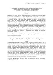
1.1 Case study <strong>bridge</strong><br />
In this paper, an existing six-span <strong>continuous</strong> welded plate girder <strong>railway</strong> <strong>bridge</strong> located in<br />
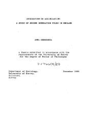
Stockholm has been taken to carryout the <strong>FE</strong> analyses. Figure 1 shows the plan <strong>and</strong> elevation <strong>of</strong> the<br />
<strong>bridge</strong>. This <strong>bridge</strong> was built over the stream Söderström in the mid-1950s to connect the northern <strong>and</strong><br />
southern Sweden with two separate train tracks laid over wooden sleepers resting on the stringer beams.<br />
Almost 520 trains pass over this <strong>bridge</strong> every day, out <strong>of</strong> which commuter trains are the most frequent<br />
whereas the freight trains are comparatively much less frequent.<br />
4 5 6<br />
7 8 9 10<br />
RB RB<br />
MWL RB RB RB RB FB<br />
27.0 m<br />
33.7 m<br />
33.7 m<br />
33.7 m 33.6 m 26.9 m<br />
18.9 m<br />
(a) Elevation view (RB – Roller Bearing <strong>and</strong> FB – Fixed Bearing)<br />
4 5 6 7 8 9 10<br />
(b) Plan view (<strong>FE</strong> Model)<br />
Figure 1. Bridge over the Söderström in Stockholm, Sweden<br />
The individual spans <strong>of</strong> the unballasted <strong>bridge</strong> vary in length between 26.9m <strong>and</strong> 33.7m. The<br />
superstructure is composed <strong>of</strong> two main girders with 3.0 m deep <strong>and</strong> 0.6 m wide built-up I section. The<br />
floor-system consists <strong>of</strong> floor beams (1.120 m by 0.330 m), <strong>and</strong> stringers (0.450 m by 0.225 m). The<br />
cross beams have an orientation with the main girder at a skew angle <strong>of</strong> 80˚. Inner <strong>and</strong> outer transverse<br />
web stiffeners are fillet-welded to main girders at equal spaces <strong>of</strong> 3.37 m. Bracings are provided at two<br />
levels, one at the top to connect the rails <strong>and</strong> other at the bottom to connect the cross beams. Additional<br />
details regarding the <strong>bridge</strong> can be found in [2].<br />
1.2. Field measurements<br />
The division <strong>of</strong> structural design <strong>and</strong> <strong>bridge</strong>s at the Royal Institute <strong>of</strong> Technology, Sweden (KTH)<br />
conducted field tests by passing a Rc6 locomotive over one track (west side track) <strong>of</strong> the <strong>bridge</strong>. The<br />
locomotive had a total weight <strong>of</strong> 78 tons <strong>and</strong> 4 axles with distances 2.7m+5.0m+2.7m. Strains <strong>and</strong><br />
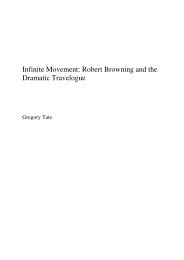
accelerations were measured at different locations <strong>of</strong> span 7–8 (see Figure 1), underneath the loaded<br />
track <strong>of</strong> the <strong>bridge</strong>, using 56 strain gauges <strong>and</strong> 5 accelerometers. Details <strong>of</strong> the strain gauge locations in<br />
span 7–8 are shown in Figure 2a.<br />
S1<br />
S2<br />
225<br />
S3<br />
12 412 450<br />
S4<br />
20<br />
225<br />
18<br />
S1, S2, S3<strong>and</strong> S4 are strain gauges
(a) Plan view at mid-span<br />
(b) Cross-section at location-C<br />
Figure 2. Details <strong>of</strong> the strain gauge locations at <strong>bridge</strong> span 7–8<br />
Measurements were obtained at stringer <strong>and</strong> cross-girder mid-spans (points C, D, I), on the main<br />
girder (point A) <strong>and</strong> at the connection between the stringer <strong>and</strong> the cross-girder (point E). Figure 2b<br />
shows a typical cross section <strong>of</strong> a stringer mid-span location with the measurements points. As can be<br />
seen, measurements at four points (two on the top flange <strong>and</strong> two on the bottom flange) have been<br />
obtained. This was the case <strong>of</strong> all members i.e. stringers, cross-girders, <strong>and</strong> main girders. The field<br />
measurements for the Rc6 locomotive were conducted at different speeds i.e. 1, 10 <strong>and</strong> 52 km/h, the<br />
first speed (1 km/h) representing effectively the case <strong>of</strong> static loading. The MGC plus system with<br />
amplifiers <strong>of</strong> the ML801 type produced by Hottinger Baldwin Messtechnik was used for the data<br />
acquisition. Measurements were recorded at 400Hz.<br />
1.3. Finite element model<br />
The dynamic behaviour <strong>of</strong> the case study <strong>bridge</strong> was investigated under different degrees <strong>of</strong> complexity,<br />
using shell <strong>and</strong>/or beam elements. <strong>FE</strong> models <strong>of</strong> the <strong>bridge</strong> were developed using the commercial <strong>FE</strong><br />
package ABAQUS [3]. Eight-noded, reduced integration shell elements (S8R) <strong>and</strong> three-noded,<br />
quadratic beam elements (B32) were used in the <strong>FE</strong> models. Single-span, three-span <strong>and</strong> six-span (full)<br />
<strong>bridge</strong> <strong>FE</strong> models were developed <strong>and</strong> analysed. Both simply supported (SS) <strong>and</strong> fixed support<br />
conditions were assumed in the single-span <strong>and</strong> three-span models at the two ends <strong>of</strong> the <strong>bridge</strong> in order<br />
to investigate the effect <strong>of</strong> boundary conditions. All members were tied to each other which are<br />
equivalent to assuming rigid connections between them.<br />
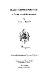
As a first step, only span (7–8) <strong>of</strong> the full <strong>bridge</strong> was modelled first with shell elements <strong>and</strong> then<br />
with beam elements. The effect <strong>of</strong> bracings was also investigated via the single-span <strong>FE</strong> model by<br />
developing a shell model with <strong>and</strong> without bracings. Figure 3a shows the shell-element model <strong>of</strong> the<br />
single span with the bracings included. In all the shell-element models, the stiffeners in the main girders<br />
were also modelled. The effect <strong>of</strong> adjacent spans in the overall behaviour <strong>of</strong> the <strong>bridge</strong> was studied by<br />
developing three-span <strong>and</strong> six-span <strong>bridge</strong> models. In the case <strong>of</strong> the three-span <strong>bridge</strong> models, one<br />
model was developed using shell elements for all spans, as shown in Figure 3b, whereas the other<br />
model was developed by a combination <strong>of</strong> shell <strong>and</strong> beam elements. In the latter model, see Figure 3c,<br />
it can be seen that shell elements were employed for span 7–8, whereas beam elements were used to<br />
model the adjacent two spans. For the full <strong>bridge</strong> model, which is shown in Figure 3d, shell elements<br />
were used only for span 7–8, the remaining spans being modelled with beam elements. In both the<br />
three-span <strong>and</strong> six-span <strong>FE</strong> models, the intermediate supports were modelled as simply supported. Due<br />
to the high computational effort required, a full-shell model <strong>of</strong> the entire <strong>bridge</strong> was not attempted.<br />
2. <strong>FE</strong> ANALYSES OF CASE STUDY BRIDGE<br />
Eigenvalue analyses were carried out on all <strong>FE</strong> models <strong>of</strong> the <strong>bridge</strong> <strong>and</strong> the results, in the form <strong>of</strong><br />
<strong>bridge</strong> periods (frequencies), were obtained <strong>and</strong> compared in order to assess the capability <strong>of</strong> different<br />
<strong>FE</strong> modelling detail levels on capturing fundamental dynamic properties <strong>of</strong> the <strong>bridge</strong>. Following the<br />
eigenvalue <strong>analysis</strong>, which was employed to obtain the fundamental dynamic properties <strong>of</strong> the <strong>bridge</strong>,
static <strong>and</strong> dynamic <strong>FE</strong> analyses under the passage <strong>of</strong> the Rc6 test locomotive were carried out to<br />
investigate its overall dynamic behaviour.<br />
2.1. Eigenvalue <strong>analysis</strong> <strong>of</strong> <strong>bridge</strong><br />
To avoid the <strong>bridge</strong> structural resonance, the fundamental frequencies <strong>of</strong> the <strong>bridge</strong> structure should<br />
not match with the excitation frequency (ν/ℓ). This depends on the speed (ν) <strong>of</strong> the passing train <strong>and</strong> the<br />
<strong>bridge</strong> span (ℓ). Eigenvalues <strong>of</strong> an undamped mechanical system can be calculated based on the<br />
equation <strong>of</strong> motion as given in Frỳba [4]. The <strong>bridge</strong> frequencies obtained from the <strong>FE</strong> <strong>analysis</strong> were<br />
compared with available empirical formulae suggested by Frỳba [4] <strong>and</strong> the International Union <strong>of</strong><br />
Railways [5]. These empirical expressions were developed through statistical evaluation <strong>and</strong> regression<br />
<strong>analysis</strong> <strong>of</strong> a large number <strong>of</strong> field measurements <strong>of</strong> <strong>bridge</strong> frequencies carried out in the past on<br />
different type <strong>of</strong> ballasted <strong>and</strong> unballasted <strong>bridge</strong>s such as <strong>steel</strong> truss, plate girder, <strong>and</strong> concrete [4].<br />
(a) Single-span shell element <strong>bridge</strong> (b) Three-span shell element <strong>bridge</strong><br />
(c) Three-span beam <strong>and</strong> shell element <strong>bridge</strong> (d) Six-span beam <strong>and</strong> shell element <strong>bridge</strong><br />
Figure 3. <strong>FE</strong> models <strong>of</strong> the <strong>bridge</strong><br />
2.2. <strong>Dynamic</strong> <strong>analysis</strong> <strong>of</strong> <strong>bridge</strong><br />
Two different types <strong>of</strong> dynamic analyses i.e. modal dynamic <strong>and</strong> implicit dynamic were undertaken<br />
to investigate the suitability <strong>of</strong> each to capture the dynamic behaviour <strong>of</strong> the <strong>bridge</strong>. Explicit dynamic<br />
<strong>analysis</strong> is computationally much more dem<strong>and</strong>ing than implicit analyses. Due to the large nature <strong>of</strong> the<br />
<strong>FE</strong> model, this type <strong>of</strong> <strong>analysis</strong> was excluded from this investigation. The difference between implicit<br />
<strong>and</strong> explicit dynamic <strong>analysis</strong> lies in the solution procedure <strong>of</strong> the dynamic equations <strong>of</strong> motion [3].
The fundamental equation <strong>of</strong> motion <strong>of</strong> the <strong>bridge</strong> system can be expressed in general form as given in<br />
Frỳba [4].<br />
The analyses were carried out on the full-span, beam-shell element <strong>FE</strong> model <strong>of</strong> the <strong>bridge</strong> (Figure<br />
3d). A range <strong>of</strong> different train velocities were employed in the analyses <strong>and</strong> the results were compared<br />
with the available field measurements. The <strong>bridge</strong> was loaded with the test locomotive <strong>and</strong> the axle<br />
loads <strong>of</strong> the train (195kN) were applied directly to the top flange <strong>of</strong> the stringers ignoring any load<br />
distribution due to the effect <strong>of</strong> rails <strong>and</strong> sleepers. Loading was initiated from the start <strong>of</strong> span 5–6 since<br />
the field measurements showed that the investigated span 7–8 experienced the effect <strong>of</strong> the locomotive<br />
from that point onwards. It was then traversed in 1m steps until the middle <strong>of</strong> span 6–7 from which<br />
point onwards a smaller step size <strong>of</strong> 0.5m was used up to the middle <strong>of</strong> span 8–9 where the step was<br />
once again changed to 1m until the locomotive exited the <strong>bridge</strong>. The loads were applied as triangular<br />
distribution <strong>of</strong> forces as suggested in [6] <strong>and</strong> [7]. An artificial damping <strong>of</strong> 5%, a typical value for this<br />
type <strong>of</strong> <strong>bridge</strong>s, was included by default in the implicit <strong>analysis</strong>. The modal dynamic <strong>analysis</strong> was<br />
carried out using 30 modes <strong>and</strong> a material damping ratio <strong>of</strong> ζ = 2.6% which was obtained based on the<br />
first modal frequency <strong>of</strong> the full <strong>bridge</strong> [4]. A static <strong>analysis</strong> <strong>of</strong> the <strong>bridge</strong> was also carried out to<br />
compare the results with the field measurements obtained under a train velocity <strong>of</strong> 1 km/h which can<br />
effectively be considered as static loading.<br />
3. RESULTS AND DISCUSSIONS<br />
(a) SS boundary conditions (b) Fixed boundary conditions<br />
Figure 4. First mode shape <strong>of</strong> the single-span shell element <strong>FE</strong> model without bracings<br />
3.1 Eigenvalue <strong>analysis</strong> <strong>of</strong> <strong>bridge</strong><br />
Single-span <strong>bridge</strong><br />
As a first step, only the span <strong>of</strong> the <strong>bridge</strong> where the field measurements were obtained (span 7–8,<br />
see Fig. 1) was modelled as a single span using shell elements. Figure 4 shows the first mode shape<br />
behaviour <strong>of</strong> the <strong>bridge</strong> model without bracings, for two different boundary conditions i.e. simply<br />
supported (SS) <strong>and</strong> fixed, whereas Figure 5 shows the first mode shape behaviour <strong>of</strong> the <strong>bridge</strong> with the<br />
bracings included in the model. It can be seen from Figure 4 that the first mode shape obtained from the<br />
model without bracings is lateral bending with periods <strong>of</strong> 0.510 <strong>and</strong> 0.460 seconds for the SS <strong>and</strong> fixed<br />
boundary conditions, respectively. The addition <strong>of</strong> bracings in the model reduces the <strong>bridge</strong> period by<br />
64% <strong>and</strong> 73% for the SS <strong>and</strong> fixed boundary conditions, respectively. This is an indication <strong>of</strong> the<br />
additional stiffness that is provided by the bracings <strong>and</strong> suggests that these should be modelled for the<br />
purposes <strong>of</strong> dynamic analyses. As a result, all subsequent analyses were carried out on models which<br />
included the bracing elements.<br />
The inclusion <strong>of</strong> bracings in the <strong>bridge</strong> <strong>FE</strong> model with SS boundary conditions resulted in a<br />
vertical bending mode shape (see Figure 5). On the other h<strong>and</strong>, the mode shape in the fixed boundary<br />
condition model was found to be a combination <strong>of</strong> lateral bending <strong>and</strong> torsion (Figure 5b). This shows<br />
that the fixed boundary condition model is able to capture the out-<strong>of</strong>-plane behaviour <strong>of</strong> the main
members which was responsible for the observed fatigue cracking in the main girder web to stiffener<br />
connections. Comparing SS <strong>and</strong> fixed boundary conditions for the model with bracings, the latter<br />
results in a period which is 32% lower than the former.<br />
(a) SS boundary conditions (b) Fixed boundary conditions<br />
Figure 5. First mode shape <strong>of</strong> the single-span shell element <strong>FE</strong> model with bracings<br />
For comparison purpose with the shell element model, a beam element model <strong>of</strong> the span under<br />
consideration was also developed <strong>and</strong> analysed. Figure 6 shows the first mode shape obtained from the<br />
eigenvalue <strong>analysis</strong> which consists <strong>of</strong> vertical bending for both SS <strong>and</strong> fixed boundary conditions. The<br />
eigenvalue <strong>analysis</strong> for this model showed that, although they are computationally much cheaper, beam<br />
elements fail to capture the out-<strong>of</strong>-plane <strong>and</strong> torsional deformations <strong>of</strong> the main <strong>bridge</strong> girders.<br />
(a) SS boundary conditions (b) Fixed boundary conditions<br />
Figure 6. First mode shape <strong>of</strong> the single-span beam element <strong>FE</strong> model with bracings<br />
Three-span <strong>bridge</strong> model<br />
The full-shell, three-span <strong>bridge</strong> model shown in Figure 3b was developed as an attempt to increase<br />
the accuracy <strong>of</strong> the obtained results. Figure 7 shows the first mode shape obtained from the eigenvalue<br />
analyses for two different boundary conditions at the two ends <strong>of</strong> the <strong>FE</strong> <strong>bridge</strong> model (SS <strong>and</strong> fixed). It<br />
can be seen that, irrespective <strong>of</strong> the boundary conditions, the first mode shape captures vertical bending<br />
<strong>of</strong> the <strong>bridge</strong> (Figures 8a <strong>and</strong> 8b). The fixed boundary condition results in a 20% reduction in the first<br />
period as compared to the SS case (0.181 vs. 0.151 seconds). The second mode obtained from the<br />
eigenvalue <strong>analysis</strong> captures the out-<strong>of</strong>-plane flexural <strong>and</strong> torsional behaviour <strong>of</strong> the main girders for<br />
both SS <strong>and</strong> fixed boundary condition assumptions.<br />
(a) SS boundary conditions (b) Fixed boundary conditions
Figure 7. First mode shape <strong>of</strong> the three-span <strong>bridge</strong> with shell element <strong>FE</strong> model<br />
In the case <strong>of</strong> SS boundary conditions, the first period <strong>of</strong> <strong>bridge</strong> was found to be very similar to the<br />
single-span model. On the other h<strong>and</strong>, in the case <strong>of</strong> fixed boundary conditions, modelling the <strong>bridge</strong><br />
with three-spans resulted in an almost 20% increase in the <strong>bridge</strong> period as compared to the single-span<br />
model (0.123 vs. 0.151 seconds).<br />
As an attempt to reduce the time required for the <strong>analysis</strong>, the adjacent spans to the investigated<br />
span were modelled using beam elements, which are computationally cheaper than shell elements.<br />
Figure 8 shows the first mode shape for the beam <strong>and</strong> shell element three-span <strong>bridge</strong> model for both<br />
boundary conditions. It can be seen that, similar to the full-shell element model described above, the<br />
first mode shape obtained for this model is vertical bending for both types <strong>of</strong> boundary conditions (see<br />
Figure 8a <strong>and</strong> 8b). The effect <strong>of</strong> fixed boundary conditions is to reduce the first time period by 20%.<br />
Comparing the beam-shell <strong>bridge</strong> <strong>FE</strong> model with the full-shell <strong>FE</strong> model in terms <strong>of</strong> the obtained<br />
periods, it was found that the former results in a slight decrease in the period by a maximum 7%. This<br />
demonstrates the fact that, for time economy considerations, modelling the remaining spans <strong>of</strong> the<br />
<strong>bridge</strong> using beam elements does not decrease the accuracy <strong>of</strong> the results considerably.<br />
(a) SS boundary conditions (b) Fixed boundary conditions<br />
Figure 8. First mode shape <strong>of</strong> the three-span <strong>bridge</strong> with beam <strong>and</strong> shell element <strong>FE</strong> model<br />
Full <strong>bridge</strong> model<br />
Figure 9 shows the first four mode shapes obtained from the eigenvalue <strong>analysis</strong> for the full-<strong>bridge</strong><br />
<strong>FE</strong> model which was developed using shell elements for span 7–8 <strong>and</strong> beam elements for the remaining<br />
<strong>bridge</strong>. As it can be seen, the out-<strong>of</strong>-plane mode is captured here through mode 3, whereas the<br />
remaining modes all include vertical bending effects. This full-<strong>bridge</strong> model results in a fundamental<br />
period <strong>of</strong> 0.208 seconds which is considerably higher than the previous models. For the subsequent<br />
modes, small increases in the periods, as compared to the single- <strong>and</strong> three-span models, are also<br />
evident. This demonstrates the fact that for the purposes <strong>of</strong> dynamic analyses, modelling the entire<br />
<strong>bridge</strong> in the way shown in Figure 3d can be expected to provide a good prediction <strong>of</strong> the dynamic<br />
behaviour <strong>of</strong> the <strong>bridge</strong>.
Overall comparisons<br />
(a) First mode (b) Second mode<br />
(c) Third mode (d) Fourth mode<br />
Figure 9. Mode shapes <strong>of</strong> the full-<strong>bridge</strong> <strong>FE</strong> model<br />
Table 1 presents an overview <strong>of</strong> the results obtained from the eigenvalue <strong>analysis</strong> using the different<br />
finite element models. The periods <strong>of</strong> the first three modes <strong>of</strong> each model as well as the time required<br />
for each <strong>analysis</strong> <strong>and</strong> the number <strong>of</strong> elements in each <strong>FE</strong> model are shown in the table. The table clearly<br />
shows the time saving achieved by using beam elements in the model. For example, comparing the<br />
analyses time for the three-span shell element model with its beam-shell counterpart, it can be seen that<br />
the <strong>analysis</strong> time required for the latter is almost one-fifth <strong>of</strong> the time required for the former. In the<br />
case <strong>of</strong> the full-<strong>bridge</strong> model, which is a combination <strong>of</strong> shell <strong>and</strong> beam elements, the time required for<br />
the <strong>analysis</strong> in almost half <strong>of</strong> that required for the three-span shell element model <strong>and</strong> is, most probably,<br />
significantly lower than the time that would be required for a full-shell entire <strong>bridge</strong> model considering<br />
the non-linear relationship between the size <strong>of</strong> the <strong>FE</strong> model (number <strong>of</strong> elements) <strong>and</strong> <strong>analysis</strong> time.<br />
Table 1. Comparison <strong>of</strong> the periods for the different <strong>FE</strong> models<br />
No. <strong>of</strong> Spans Single-span Three-span Full <strong>bridge</strong><br />
Model Shell Element Beam Element Shell Beam-Shell Beam-shell<br />
No. <strong>of</strong><br />
elements<br />
12139 1318 35174 15231 17369<br />
Analysis time<br />
(s)<br />
292 10 1446 303 701<br />
Boundary<br />
conditions<br />
SS Fixed SS Fixed SS Fixed SS Fixed SS<br />
T1 (s) 0.182 0.123 0.176 0.114 0.181 0.151 0.178 0.142 0.208<br />
T2 (s) 0.156 0.086 0.148 0.114 0.161 0.148 0.152 0.137 0.164<br />
T3 (s) 0.110 0.066 0.115 0.114 0.146 0.131 0.140 0.116 0.145<br />
Table 2 shows the fundamental period obtained for the particular <strong>bridge</strong> being investigated through<br />
the available empirical formulae. Comparison <strong>of</strong> the empirical values with the results obtained from the<br />
<strong>FE</strong> eigenvalue analyses presented in Table 1 reveals a good agreement between the two sets <strong>of</strong> results.
The first natural frequency obtained from the full-<strong>bridge</strong> model lies well within the upper <strong>and</strong> lower<br />
limits suggested by the UIC [5] & BS EN 1991–2 [8].<br />
Table 2. Comparison <strong>of</strong> the first period T1 <strong>of</strong> the single-span <strong>FE</strong> models with available empirical formulae<br />
Single-span <strong>FE</strong> Model Frỳba [4] UIC [5] & BS EN 1991–2 [8]<br />
Shell Elements Beam Elements<br />
(1)<br />
(2)<br />
(3)<br />
(4)<br />
Boundary<br />
conditions<br />
SS Fixed SS Fixed 133× ℓ -0.9 208× ℓ -1 23.58× ℓ -0.592 94.76× ℓ -0.748<br />
T1 (s) 0.182 0.123 0.176 0.114 0.178 0.162 0.340 0.147<br />
(1)<br />
for <strong>railway</strong> <strong>bridge</strong>s <strong>of</strong> all types, materials <strong>and</strong> structural systems,<br />
(2)<br />
for <strong>steel</strong> plate girder <strong>bridge</strong>s without ballast,<br />
(3)<br />
unloaded <strong>railway</strong> <strong>bridge</strong>s <strong>of</strong> all types <strong>and</strong> materials, lower limit (for span 20 ≤ ℓ ≤ 100m) <strong>and</strong><br />
(4)<br />
unloaded <strong>railway</strong> <strong>bridge</strong>s <strong>of</strong> all types <strong>and</strong> materials, upper limit (for span 4 ≤ ℓ ≤ 100m)<br />
3.2 <strong>Dynamic</strong> <strong>analysis</strong> <strong>of</strong> <strong>bridge</strong><br />
The full-span <strong>bridge</strong> <strong>FE</strong> model was used to carry out a number <strong>of</strong> initial parametric dynamic<br />
analyses under the passage <strong>of</strong> the test locomotive <strong>and</strong> to compare the results with the available field<br />
measurements in order to determine the most appropriate type <strong>of</strong> dynamic analyses. Both implicit <strong>and</strong><br />
modal dynamic analyses using 30 modes were carried out using ABAQUS. The results obtained from<br />
the modal <strong>analysis</strong> did not show good agreement with the field measurements <strong>and</strong> hence they are<br />
excluded from further discussion. Since the available field measurements included the case <strong>of</strong> a “static”<br />
passage <strong>of</strong> the test locomotive over the <strong>bridge</strong> by a velocity <strong>of</strong> 1 km/h, a static <strong>FE</strong> <strong>analysis</strong> <strong>of</strong> the <strong>bridge</strong><br />
was also carried out.<br />
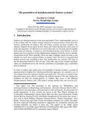
Figure 10 shows the comparison <strong>of</strong> the strain histories obtained from the static <strong>analysis</strong> with the<br />
field measurements at points S1 <strong>and</strong> S2 <strong>of</strong> location C (see Figure 3), which is located at the mid-length<br />
<strong>of</strong> the stringer, under a velocity <strong>of</strong> 1 km/h. It can be seen that good overall agreement between the<br />
results is obtained with the static <strong>FE</strong> <strong>analysis</strong> predicting slightly higher maximum strains at the peak<br />
points.<br />
Strain<br />
0.00015<br />
0.0001<br />
0.00005<br />
-0.00005<br />
-0.0001<br />
-0.00015<br />
Location C<br />
0<br />
0 10 20 30 40 50 60 70 80 90 100<br />
Time (s)<br />
Measured<br />
<strong>FE</strong>-Static<br />
Location C<br />
Figure 10. Comparison <strong>of</strong> the strains between field measurements (1km/h) <strong>and</strong> <strong>FE</strong> <strong>analysis</strong><br />
Figure 11 shows the comparison <strong>of</strong> strain histories obtained from the implicit dynamic <strong>analysis</strong><br />
under velocities <strong>of</strong> 10 km/h with the field measurements under the same speeds. Similar comparison<br />
was made for train velocity <strong>of</strong> 52 km/h. Good agreement can be seen between the results in the case <strong>of</strong><br />
the dynamic analyses with very good prediction <strong>of</strong> the maximum strains. Although the implicit dynamic<br />
<strong>analysis</strong> captures the overall trend <strong>of</strong> the strain history well, it produces some additional smaller strain<br />
cycles which is, however, expected to be insignificant in terms <strong>of</strong> fatigue assessment <strong>and</strong> fatigue<br />
damage calculations.<br />
Strain<br />
0.00015<br />
0.0001<br />
0.00005<br />
-0.00005<br />
-0.0001<br />
-0.00015<br />
0<br />
0 10 20 30 40 50 60 70 80 90 100<br />
Time (s)<br />
(a) Left top (S1) (b) Left Bottom (S2)<br />
Measured<br />
<strong>FE</strong>-Static
Strain<br />
0.0002<br />
0.00015<br />
0.0001<br />
0.00005<br />
-0.00005<br />
-0.0001<br />
-0.00015<br />
Location C<br />
0<br />
10 15 20 25 30 35 40 45 50<br />
Time (s)<br />
Measured<br />
<strong>FE</strong>-Implicit<br />
Figure 11. Comparison <strong>of</strong> the strains between field measurements (10km/h) <strong>and</strong> <strong>FE</strong> <strong>analysis</strong><br />
Mean stress ranges<br />
The mean stress range E[Sr] at a detail can be viewed as an important parameter in terms <strong>of</strong> fatigue<br />
assessment. The strain histories obtained from the passage <strong>of</strong> the test locomotive over the <strong>bridge</strong> were<br />
converted in stress histories <strong>and</strong> these were then analysed using the rainflow counting procedure to<br />
obtain the stress range histogram <strong>and</strong>, therefore, E[Sr]. Mean stress ranges obtained at the mid-span <strong>of</strong><br />
the stringer <strong>and</strong> cross-girder, connections <strong>of</strong> the stringer with cross-girder <strong>and</strong> the main girder near to<br />
the loaded track <strong>of</strong> the <strong>bridge</strong> were compared. Locomotive speed <strong>of</strong> 1km/h (static case) shows that the<br />
stress ranges obtained from the <strong>FE</strong> static <strong>analysis</strong> are generally more conservative. The highest<br />
deviations were observed at the location <strong>of</strong> stringer mid-span.<br />
There is a better agreement between the results obtained from the dynamic <strong>FE</strong> <strong>analysis</strong> <strong>and</strong> the field<br />
measurements for velocities <strong>of</strong> 10 <strong>and</strong> 52 km/h. The mean stress ranges obtained from the stringers <strong>of</strong><br />
the <strong>bridge</strong> were higher than the cross-girder <strong>and</strong> main-girder. Overall, a good agreement <strong>of</strong> the mean<br />
stress range between field measurements <strong>and</strong> dynamic <strong>FE</strong> <strong>analysis</strong> under higher velocities is an<br />
indication that the fatigue life may be estimated with reasonable accuracy through results obtained from<br />
the <strong>FE</strong> model <strong>of</strong> a <strong>bridge</strong> in the form <strong>of</strong> Figure 3d.<br />
4. CONCLUSIONS<br />
For the case-study <strong>bridge</strong>, first the effect <strong>of</strong> modelling assumptions on dynamic behaviour were<br />
investigated on a number <strong>of</strong> different <strong>FE</strong> models by the eigenvalue analyses. It was found that<br />
secondary elements such as bracings may have a significant effect on the frequency <strong>of</strong> the <strong>bridge</strong> <strong>and</strong> it<br />
is suggested that they are modelled during an <strong>FE</strong> <strong>analysis</strong>. It was also found that in order to capture the<br />
out-<strong>of</strong>-plane <strong>and</strong> torsional behaviour <strong>of</strong> the main girders, which lead to the development <strong>of</strong> fatigue<br />
cracks on the case-study <strong>bridge</strong>, shell elements should be used in the <strong>FE</strong> models, as beams are unable to<br />
capture such type <strong>of</strong> behaviour. Modelling the investigated span <strong>of</strong> a <strong>bridge</strong> using shell elements <strong>and</strong> the<br />
remaining spans using beam elements is suggested as an economical <strong>and</strong> practical way <strong>of</strong> obtaining<br />
reasonably accurate results. Overall, good agreement between the dominant <strong>bridge</strong> frequencies obtained<br />
from the eigenvalue <strong>analysis</strong> <strong>and</strong> empirical results was observed. Later the full-<strong>bridge</strong> <strong>FE</strong> model was<br />
analysed dynamically under the passage <strong>of</strong> the test locomotive with different velocities. The comparison<br />
<strong>of</strong> the results obtained from dynamic <strong>FE</strong> analyses with available field measurements showed that<br />
implicit dynamic <strong>analysis</strong> is a reasonable <strong>and</strong> computationally efficient method <strong>of</strong> capturing the<br />
dynamic behaviour <strong>of</strong> a <strong>bridge</strong> <strong>and</strong> obtaining dynamic stress histories.<br />
ACKNOWLEDGEMENTS<br />
This work was carried out with a financial grant from the Research Fund for Coal <strong>and</strong> Steel (RFCS)<br />
<strong>of</strong> the European Community, granted under the contract Nr. RFSR-CT-2008-00033. The authors<br />
sincerely acknowledge the division <strong>of</strong> structural design <strong>and</strong> <strong>bridge</strong>s at the Royal Institute <strong>of</strong> Technology<br />
0.0002<br />
0.00015<br />
0.0001<br />
0.00005<br />
-0.00005<br />
-0.0001<br />
-0.00015<br />
-0.0002<br />
Location C<br />
0<br />
10 15 20 25 30 35 40 45 50<br />
(a) Left top (S1) (b) Left Bottom (S2)<br />
Strain<br />
Time (s)<br />
Measured<br />
<strong>FE</strong>-Implicit
(KTH) Sweden, structural engineering division at the Chalmers University <strong>of</strong> Technology Sweden <strong>and</strong><br />
the Swedish Rail administration for providing the field measurements.<br />
RE<strong>FE</strong>RENCES<br />
[1] Pipinato A., Pellegrino C., Bursi O.S., Modena C.: High-cycle fatigue behaviour <strong>of</strong> riveted<br />
connections for <strong>railway</strong> metal <strong>bridge</strong>s. Journal <strong>of</strong> Constructional Steel Research 65(2009), 12,<br />
2167–2175.<br />
[2] Le<strong>and</strong>er J., Andersson A., Karoumi R.: Monitoring <strong>and</strong> enhanced fatigue evaluation <strong>of</strong> a <strong>steel</strong><br />
<strong>railway</strong> <strong>bridge</strong>. Engineering Structures 32 (2010), 3, 854–863.<br />
[3] ABAQUS. St<strong>and</strong>ard User’s Manual Version 6.9–1. Hibbitt Karlsson & Sorensen, Inc., 2009.<br />
[4] Frỳba L.: <strong>Dynamic</strong>s <strong>of</strong> Railway Bridges. Thomas Telford, London 1996.<br />
[5] UIC 776–1 R. Loads to be considered in the design <strong>of</strong> <strong>railway</strong> <strong>bridge</strong>s. International Union <strong>of</strong><br />
Railways, 1979.<br />
[6] Gu G., Kapoor A., Lilley D M.: Calculation <strong>of</strong> dynamic impact loads for <strong>railway</strong> <strong>bridge</strong>s using a<br />
direct integration method. Proc. Inst Mech Eng Part F: J Rail <strong>and</strong> Rapid Transit (2008), 222, 385–<br />
398.<br />
[7] Goicolea J. M., Dominguez J., Navarro J. A., Gabaldon F.: New dynamic <strong>analysis</strong> methods for<br />
<strong>railway</strong> <strong>bridge</strong>s in codes IAPF <strong>and</strong> Eurocode 1. Proceedings <strong>of</strong> IABSE: Railway Bridges: Design,<br />
Construction <strong>and</strong> Maintenance, Madrid 2002.<br />
[8] BS EN 1991–2: 2003, Eurocode 1: Actions on Structures – Part 2: Traffic loads on <strong>bridge</strong>s. British<br />
St<strong>and</strong>ard Institution, UK: London.