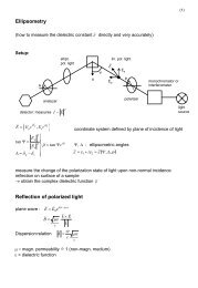
Magnetism 1
Magnetism 1
Magnetism 1

Create successful ePaper yourself
Turn your PDF publications into a flip-book with our unique Google optimized e-Paper software.
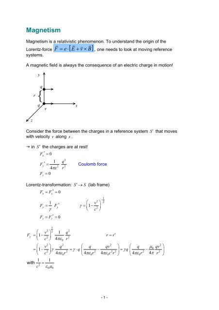
<strong>Magnetism</strong><br />
<strong>Magnetism</strong> is a relativistic phenomenon. To understand the origin of the<br />
, one needs to look at moving reference<br />
Lorentz-force F = e⋅ [ E+ v× B]<br />
systems.<br />
A magnetic field is always the consequence of an electric charge in motion!<br />
z<br />
y<br />
r { q<br />
q<br />
v<br />
x<br />
Consider the force between the charges in a reference system S′ that moves<br />
with velocity v along x .<br />
in S′ the charges are at rest!<br />
F ′ = 0<br />
x<br />
1<br />
F ′<br />
y =<br />
4πε<br />
F = 0<br />
z<br />
q<br />
2<br />
2 2<br />
r<br />
Coulomb force<br />
Lorentz-transformation: S′ → S (lab frame)<br />
F = F′<br />
= 0<br />
x x<br />
1<br />
2<br />
−<br />
2<br />
1<br />
⎛ v ⎞<br />
Fy = F ′<br />
y γ =⎜1− 2 ⎟<br />
γ<br />
⎝ c ⎠<br />
F = F′<br />
= 0<br />
z z<br />
2<br />
1<br />
2<br />
2<br />
⎛ v ⎞ 1 q<br />
Fy= ⎜1− ⎟<br />
r = r′<br />
⎝ c ⎠ 4πε<br />
r<br />
2 2<br />
0<br />
2 2 2<br />
⎛ ⎞ ⎛ ⎞ ⎛<br />
v q q<br />
= ⎜1− 2 ⎟γ = γ ⋅q 2 ⎜ 2<br />
⎝ c ⎠ 4πε 0r ⎝4πε 0r qv q<br />
− q<br />
2 2 ⎟= γ ⎜ 2<br />
4πε 0c r ⎠ ⎝4πε<br />
0r<br />
µ 0 qv<br />
− 2<br />
4π<br />
r<br />
1<br />
with 2<br />
c<br />
1<br />
=<br />
εµ<br />
0 0<br />
- 1 -<br />
2<br />
⎞<br />
⎟ ⎠
now for vc γ ≈ 1<br />
⎛ q ⎛−µ 0 ⎞ qv⎞<br />
→Fy≈ q⎜ + v⋅<br />
2 ⎜ ⎟⋅<br />
2 ⎟<br />
⎝4πε 0r<br />
⎝ 4π<br />
⎠ r ⎠<br />
<br />
Eel v⋅B<br />
<br />
in vector form: v = v ⋅xˆ<br />
2 ⎡ µ 0qv<br />
⎤<br />
= q⎢Eyˆ− ( xˆ zˆ)<br />
2<br />
4π<br />
r<br />
− × ⎥<br />
⎢⎣ yˆ<br />
⎥⎦<br />
<br />
( <br />
µ<br />
)<br />
0qv<br />
= q E+ v× B , where Bz=<br />
2<br />
4π<br />
r<br />
→ F = q⋅ ( <br />
v× B)<br />
mag<br />
Classical picture<br />
Magnetic moments originate from circular electric currents.<br />
<br />
<br />
1 ⎛ r ⎞<br />
Biot-Savat: δH = ⋅I⋅ δs<br />
2 ⎜ × ⎟<br />
4π<br />
r ⎝ r ⎠<br />
e<br />
ds <br />
magnetic moment originates from a circular current loop<br />
dµ = I⋅d <br />
S<br />
<br />
µ =<br />
<br />
dS =<br />
magnetic moment<br />
surface enclosed by the current<br />
<br />
2<br />
µ = I dA = 4πr<br />
⋅I<br />
∫ <br />
for a circular loop<br />
r<br />
4π<br />
e 2<br />
= r ;<br />
τ<br />
e<br />
I =<br />
τ<br />
for the case of an electron circulating around a ring with period τ<br />
This can be related to the angular momentum of the electron.<br />
<br />
le = r× p = r× ve⋅ me 2π<br />
r<br />
where v=<br />
τ<br />
2<br />
2π<br />
r<br />
= me<br />
τ<br />
e<br />
⇒ µ =− ⋅le 2me<br />
<br />
relation between angular momentum and magnetic moment of a<br />
circulating electron<br />
They are antiparallel because of the negative charge of the electron.<br />
- 2 -
Of course within an atom the orbit of the electron cannot be described in a<br />
classical way.<br />
⇒ Quantum mechanical description of the hydrogen atom<br />
H<br />
E<br />
0<br />
p<br />
e -<br />
pˆ Ze<br />
= −<br />
m r<br />
2 e<br />
2 2<br />
( ) 2<br />
2 4<br />
mZ e Ze<br />
=− =−<br />
2n 2a<br />
⋅n<br />
o<br />
n<br />
e<br />
2 2 2<br />
0<br />
2<br />
<br />
−10<br />
a0=<br />
≈ 0.529× 10<br />
2<br />
me<br />
o o<br />
2<br />
e<br />
1 0<br />
2a0<br />
E − E = = 1 Ry = 13.6 eV<br />
spherical coordinates:<br />
n = 1,2,...<br />
( r, ϑϕ , ) R ( r) Y ( ϑϕ , )<br />
Ψ nlm =<br />
ne <br />
nlm<br />
l = 0,..., n−1<br />
m= - l,..., + l<br />
Laguerre spherical<br />
polynom harmonic<br />
main quantum number<br />
orbital quantum number<br />
magnetic quantum number<br />
n-fold degeneracy of electronic levels<br />
m “Bohr radius”<br />
H ° has sperical symmetry<br />
→Ψ are eigenstates of the orbital angular momentum operator<br />
nlm<br />
lˆ= rˆ× pˆ<br />
Motion in a magnetic field<br />
q <br />
p → ∇− A<br />
i c<br />
H =∇× A<br />
<br />
LˆΨ = l( l+<br />
1)<br />
Ψ<br />
nlm nlm<br />
2 2<br />
LˆΨ = l( l+<br />
1)<br />
Ψ<br />
nlm nlm<br />
LˆΨ = mΨ<br />
z nlm nlm<br />
A magnetic vector potential<br />
magnetic field<br />
<br />
Recall: A is not uniquely defined: A′ = A+∇χ <br />
→∇× A′ =∇× A+∇×∇<br />
<br />
χ<br />
≡0<br />
<br />
= H<br />
<br />
have to chose transverse gauge where ∇ A = 0<br />
- 3 -<br />
χ: scalar field
Also in general we have to watch out because A and ∇ do not commute.<br />
<br />
∇A−A∇≠0 <br />
∇A Ψ −A∇ Ψ ≠0<br />
The good thing is, in the transverse gauge they do commute<br />
2 2<br />
⎛ e ⎞ 2 e <br />
e 2<br />
→⎜ ∇+ A⎟ =−∆+ 2 A∇+<br />
A 2<br />
⎝ i c ⎠<br />
i c c<br />
2 2<br />
− e 1 e 2<br />
<br />
2 Z⋅e ⇒ H = ∆+ A⋅∇+ A − 2<br />
2me i cme 2me<br />
c r<br />
1 <br />
transverse gauge ⇒ A ( <br />
= H× r)<br />
2<br />
2 2<br />
−<br />
e 2<br />
⇒ ( <br />
)<br />
e <br />
H r ( <br />
H r)<br />
Ze<br />
H = ∆+ × ⋅∇+ × −<br />
2<br />
2me i mec 8mc<br />
r<br />
<br />
cyclic property ( <br />
H× r) ⋅∇= ( <br />
r×∇) ⋅H<br />
recognize that r× p = l<br />
op. of angular momentum<br />
<br />
<br />
<br />
r× ∇ = l<br />
i<br />
with the definition<br />
e⋅<br />
<br />
= µ B<br />
2m<br />
e<br />
and p<br />
i ∇→<br />
<br />
µ = 9.274⋅ 10<br />
B<br />
2 nd term:<br />
µ L⋅H <br />
B<br />
“Bohr magneton”<br />
−24<br />
2<br />
Am<br />
paramagnetic term for orbital magnetism<br />
3 rd term:<br />
<br />
assume H zˆ<br />
<br />
( 2<br />
) 2 2 2<br />
H× r = H ( x + y ) diamagnetic term<br />
2 2<br />
−<br />
c Ze<br />
= ∆+ B ⋅ + + −<br />
2<br />
2m 8me<br />
r<br />
→ ˆ z<br />
2 2 2<br />
H µ H L H ( x y )<br />
paramagnetic term<br />
diamagnetic term<br />
- 4 -<br />
2
Operator of orbital magnetic momentum:<br />
∂Hˆ<br />
ˆz<br />
ˆ µ orb =− =−µ BL<br />
−<br />
∂H<br />
2<br />
e 2 2 ( x + y ) H<br />
2<br />
4me<br />
Ψnlm z ˆ µ orb Ψnlm 2<br />
e<br />
2 2<br />
=−µ B ⋅m − ⋅H⋅ 2 Ψ nlm x + y Ψnlm<br />
<br />
4me<br />
permanent<br />
paramagnetic<br />
moment<br />
Zeeman effect<br />
a) assume Lz = 1, 2 2<br />
x + y<br />
2<br />
2 <br />
~ ao; ao<br />
=<br />
me<br />
field-induced diamagnetic moment<br />
2<br />
2 2<br />
2 2 3<br />
Ediam eH 1 x + y <br />
−6<br />
→ ≈ ⋅H ≈10 ⋅H[<br />
Tesla]<br />
2 2 3<br />
E 8mc µ H L 4me<br />
parallel B z<br />
diamagnetic contribution is negligible, only relevant in the absence of a<br />
paramagnetic moment, i.e. for L z = 0 .<br />
b) ratio of paramagnetic term to typical electronic energies:<br />
para<br />
E µ B<br />
= el<br />
E<br />
z<br />
L<br />
2<br />
e<br />
2⋅<br />
a<br />
⋅ H −6<br />
≈210 ⋅ H [ Tesla]<br />
;<br />
2<br />
e<br />
13,6 eV<br />
2a o<br />
=<br />
−5<br />
o<br />
⇒ E ~10 eV ~1K at H = 1Tesla<br />
para<br />
remember: 300K<br />
25meV<br />
1K ≈ˆ<br />
10µ<br />
eV<br />
field dependent term can be treated as weak perturbation with respect to<br />
electronic terms<br />
~> ( ˆ ˆz<br />
o<br />
H 0 + µ BHL ) Ψ nlm = ( En + mH µ B)<br />
Ψnlm<br />
<br />
∆E<br />
nlm<br />
H = 0<br />
Z<br />
H > 0<br />
m=2<br />
1<br />
0<br />
-1<br />
-2<br />
∆ E = µ B ⋅H<br />
Zeeman splitting<br />
The magnetic field lifts the degeneracy of the (n,l) shell.<br />
2l+1 sublevels split by ∆ E = µ B ⋅ H<br />
- 5 -<br />
E<br />
for l=2
In addition to the orbital magnetic momentum there is the magnetic momentum<br />
related to the spin of the electron.<br />
→ derived from a fully relativistic treatment!<br />
<br />
→ electron has an intrinsic angular momentum with quantization, spin ½ .<br />
2<br />
Sˆχs( s 1)<br />
χ<br />
<br />
<br />
z<br />
= + χ = spin part of the electron wave function<br />
or<br />
or ,<br />
( ) ( )<br />
nlm r S χ<br />
+ ½<br />
−½ Ψ = Ψ<br />
<br />
orbital part<br />
S χ = m<br />
χ m = ± ½<br />
s s<br />
2 2 3 2<br />
S χ = S( S+<br />
1)<br />
χ = χ<br />
4<br />
⇒ additional Zeeman term<br />
<br />
para<br />
=− µ ( 2ˆ)<br />
B L+ s H<br />
para<br />
Ψ =+ µ ( m + 2m<br />
) Ψ<br />
B l s<br />
spin part<br />
2 = rel. effect<br />
ms = ± 1/2<br />
Actually the spin is not represented by a vector whose components are scalars<br />
but rather by 2x2 matrices ⇒ the “Pauli-spin” matrices.<br />
⎛0 ˆ σ x = ⎜<br />
⎝1 1⎞ ⎟, 0⎠ ⎛0 σ y = ⎜<br />
⎝i −i<br />
⎞<br />
⎟, 0 ⎠<br />
⎛1 σz = ⎜<br />
⎝0 0 ⎞<br />
⎟,<br />
−1⎠<br />
ˆ σ = ( σx, σ y, σ z)<br />
be a a vector<br />
⎛ a3 ˆ σ ⋅ a =⎜<br />
⎝a1+ ia2 a1−ia2⎞ ⎟<br />
−a3<br />
⎠<br />
such matrices can be multiplied together leading to<br />
2<br />
ˆ σ ⋅ a σb = a⋅ b + iσ a× b and σa<br />
= a show in exercise<br />
( ) ( ) ( ) ( ) 2<br />
The spin angular momentum is determined as<br />
1<br />
sˆ<br />
= ˆ σ<br />
2<br />
⎛0 1⎞ ⎛0 −i<br />
⎞ ⎛1<br />
0 ⎞<br />
Sx = ⎜ ⎟, Sy = ⎜ ⎟, Sz<br />
= ⎜ ⎟<br />
2⎝1 0⎠ 2⎝i0 ⎠ 2⎝0<br />
−1⎠<br />
only Sz<br />
is diagonal<br />
↑z ⎛1⎞ = ⎜ ⎟<br />
⎝0⎠ Sˆ<br />
z ↑z 1<br />
= <br />
2<br />
↑<br />
↓z ⎛0⎞ = ⎜ ⎟<br />
⎝1⎠ ˆ 1<br />
Sz<br />
↓ = − <br />
z ↓<br />
2<br />
ms<br />
- 6 -
The eigenstates concerning spin parallel to x-axis are<br />
↑x =<br />
1 ⎛1⎞ ⎜ ⎟<br />
2 ⎝1⎠ ↓x<br />
=<br />
1<br />
2<br />
⎛ 1 ⎞<br />
⎜ ⎟<br />
⎝−1⎠ ↑y =<br />
1 ⎛1⎞ ⎜ ⎟<br />
2 ⎝i⎠ ↓y<br />
=<br />
1 ⎛ 1 ⎞<br />
⎜ ⎟<br />
2 ⎝−i⎠ ⎛1⎞ ˆ σ x ⎜ ⎟<br />
⎝1⎠ ⎛0 = ⎜<br />
⎝1 1⎞ ⎛1⎞ ⎟ ⎜ ⎟<br />
0⎠ ⎝1⎠ ⎛1⎞ = ⎜ ⎟<br />
⎝1⎠ ⎛ 1 ⎞ ⎛0 ˆ σ x′<br />
⎜ ⎟= ⎜<br />
⎝−1⎠ ⎝1 1⎞ ⎛ 1 ⎞<br />
⎟ ⎜ ⎟<br />
0⎠ ⎝− 1⎠ ⎛−1⎞ = ⎜ ⎟<br />
⎝+ 1⎠ ⎛ 1 ⎞<br />
= ( −1)<br />
⎜ ⎟<br />
⎝− 1⎠<br />
⎛1⎞ ˆ σ y ⎜ ⎟<br />
⎝i⎠ ⎛0 = ⎜<br />
⎝i −i<br />
⎞ ⎛1⎞ ⎟ ⎜ ⎟<br />
0 ⎠ ⎝i⎠ ⎛1⎞ = ⎜ ⎟<br />
⎝i⎠ ⎛ 1 ⎞ ⎛0 σ y ⎜ ⎟ = ⎜<br />
⎝−i⎠ ⎝i −i⎞ ⎛ 1 ⎞<br />
⎟ ⎜ ⎟<br />
0 ⎠ ⎝−i⎠ ⎛−1⎞ = ⎜ ⎟<br />
⎝ i ⎠<br />
⎛1⎞ = ( −1)<br />
⎜ ⎟<br />
⎝i⎠ → This two-component representation of the spin wave functions is known as a<br />
spinor representation. The eigenstates are referred to as spinors.<br />
⎛a⎞ A general spin state can be written as χ = ⎜ ⎟=<br />
a ↑ + b z ↓z<br />
⎝b⎠ 2 2<br />
normalization → a + b = 1<br />
The total angular spin operator is determined as Sˆ ( Sˆ , ˆ , ˆ<br />
x Sy Sz)<br />
vector of 2x2 matrices!<br />
2<br />
→ Sˆ= S<br />
2<br />
+ S<br />
2<br />
+ S<br />
2<br />
( x y z )<br />
( x y z )<br />
2<br />
S χ =<br />
2 2 2<br />
S + S + S<br />
⎛1 1 1⎞ χ = ⎜ + + ⎟<br />
⎝4 4 4⎠ 3<br />
χ = χ<br />
4<br />
2<br />
→ S<br />
3<br />
χ = χ = s( s+ 1)<br />
χ<br />
4<br />
1⎛1 ⎞ 3<br />
⎜ + 1⎟=<br />
2⎝2 ⎠ 4<br />
= . This is a<br />
Commutation relations<br />
⎡Sˆ , ˆ ˆ ˆ ˆ ˆ ˆ<br />
x S ⎤ y = SxSy − SySx = iS<br />
you have to watch out which operator is first<br />
⎣ ⎦<br />
z<br />
applied to the wave function.<br />
ˆ 2<br />
and ⎡⎣S , S ⎤ z ⎦ = 0<br />
The components do not commute with each other; each component commutes<br />
with ˆS<br />
2<br />
.<br />
- 7 -
Raising and lowering operators<br />
The origin of the spin degree of freedom: relativistic energy–momentum<br />
relationship<br />
2 2 2 2 4<br />
E = c p + m c<br />
1<br />
2<br />
−<br />
2<br />
⎛ v ⎞<br />
p= γ ⋅ mv,<br />
γ = ⎜1− 2 ⎟<br />
⎝ c ⎠<br />
∂<br />
E →i, ∂t<br />
<br />
p→<br />
∇<br />
i<br />
correspondence principle<br />
4-dimensional covariant form (treat time and space the same way)<br />
<br />
P → iδµ<br />
4-dimensional vector<br />
µ<br />
⎛ E ⎞<br />
Pµ = ⎜γmv, ⎟<br />
⎝ c ⎠<br />
⎛ 1 ∂ ⎞<br />
∂ µ = ⎜−∇, c γ t<br />
⎟<br />
⎝ ⎠<br />
→ Klein–Gordon equation:<br />
2 2 4<br />
⎛ ⎞<br />
1 ∂ mc<br />
⎜∆−<br />
− Ψ= 0<br />
2 2 2 ⎟<br />
⎝ c ∂t<br />
⎠<br />
This is a differential equation of the second kind in time and space<br />
∂Ψ<br />
→ the solution requires starting values for Ψ and<br />
γ t<br />
Conclusion: This cannot be!<br />
Dirac’s idea: linearize the equation<br />
2 2<br />
E−c α 0<br />
( ipi − βmc ⎛E c α )<br />
jpj βmc<br />
⎞<br />
⎜<br />
+ +<br />
⎟<br />
i ⎝ j<br />
⎠<br />
this agrees with the Klein–Gordon equation if<br />
α α + α α = 2δij<br />
2<br />
∑ ∑ = i, j ε { x, yz , }<br />
i j j i<br />
αβ+ βa<br />
= 0<br />
i i<br />
relativistic counterpart of<br />
Schrödinger equation<br />
β = 1<br />
cannot be fulfilled with ordinary numbers. Need to consider certain 4x4 matrices.<br />
⎛0 α = ⎜<br />
⎝σ <br />
σ ⎞ ⎛1 ⎟β =<br />
1<br />
⎜<br />
⎠ ⎝0 0⎞ ⎛0 ⎟ with σx = ⎜<br />
1⎠ ⎝1 1⎞ ⎛0 ⎟, σ y = ⎜<br />
0⎠ ⎝i −i<br />
⎞ ⎛1<br />
⎟, σz<br />
= ⎜<br />
0 ⎠ ⎝0<br />
0 ⎞<br />
⎟<br />
−1⎠<br />
2<br />
→ each solution to E∓c 0<br />
( ∑αipi<br />
∓ β mc = is thus also a solution to the Klein–<br />
)<br />
Gordon equation.<br />
→ Dirac’s equation for rel. free particle<br />
⎛ ∂ ⎞<br />
⎜i−cαp−βmc⎟Ψ = 0<br />
⎝ ∂t<br />
⎠<br />
i<br />
- 8 -
The wave function now takes four components:<br />
⎛Ψ1⎞ ⎫<br />
↑<br />
⎜ ⎟ ⎬particle<br />
Ψ2 ⎭<br />
↓<br />
Ψ= ⎜ ⎟<br />
⎜Ψ⎟ 3 ⎫<br />
↑<br />
⎜ ⎟ ⎬anti-particles<br />
Ψ ↓<br />
⎝ 4 ⎠ ⎭<br />
Return to the ordinary Schrödinger equation when the spin is introduced “ad<br />
hoc” as an additional paramagnetic term<br />
→ still need to consider additional velocity effects.<br />
Spin-Orbit-Coupling<br />
<br />
<br />
⎛r ⎞dφ<br />
Electric field of nucleus E =−∇ φ =−⎜ ⎟ .<br />
⎝r ⎠ dr<br />
As seen by the electron, the nucleus is orbiting around it with velocity v → thus<br />
it creates a magnetic field that acts on the electron spin.<br />
<br />
−1<br />
( <br />
<br />
H )<br />
nuc = v× E<br />
∂B<br />
2<br />
c<br />
Faraday law: ∇× E =−<br />
γ t<br />
↓<br />
<br />
so<br />
∆ E = 2µ<br />
BS⋅Hnuc e1dφ =− S( <br />
v× r) 2<br />
mc r dr<br />
recall (<br />
<br />
m v× r) = î<br />
2<br />
e =− 2 2<br />
mc<br />
1 dφ<br />
s⋅l r dr<br />
= spin-orbit-coupling term<br />
This classical estimate is still wrong by a factor of 2.<br />
2<br />
so<br />
⇒ = 2 2<br />
2mc<br />
2<br />
Ze<br />
s⋅l 3<br />
r<br />
<br />
<br />
H<br />
<br />
2<br />
Ze<br />
φ =<br />
r<br />
2<br />
dφZe =−<br />
dr r<br />
<br />
→ s and l are no longer decoupled, they are no longer separately conserved<br />
quantities<br />
<br />
→ introduce total angular momentum j = l + s<br />
j = l− s , ..., l+ s , 2 j+<br />
1 values<br />
<br />
2 2 2 2 2 2<br />
J = L + S + 2SL→ 2SL<br />
= J −L −S<br />
so λ<br />
→ ( 2 2 2<br />
H = J −L −S<br />
)<br />
2<br />
2 2<br />
Ze<br />
λ = 2 2 3<br />
mc r<br />
<br />
= spin-orbit-coupling constant<br />
large Z → λ is very large, even larger than the paramagnetic terms in lab fields<br />
for very large Z (heavy elements).<br />
so<br />
∆ E ~1K for Z = 1, but ~ Z<br />
2<br />
- 9 -
( )<br />
0 so Z Z<br />
B µ<br />
H = H + H + J + S H L+ 2 S = J + S since J = L+ S<br />
→ the problem is that s mixes states with different .<br />
<br />
ml, ms<br />
<br />
l, s⋅ l = i l × s)<br />
, only the Z-components are conserved.<br />
[ ] (<br />
⇒ the spin-orbit interaction lifts the degeneracy between different levels with<br />
s and l (without a magnetic field), it leads to a different kind of splitting than the<br />
<br />
Zeeman-splitting → levels with the same j-value are degenerate for some<br />
s , l .<br />
E( J) −E( J − 1) λ<br />
= ( J( J + 1) ) −<br />
2<br />
= λ ⋅J<br />
L( L+ 1) − S( S+ 1) 1<br />
−<br />
2<br />
J −1 J − L L+ 1 − S S+<br />
1<br />
for same<br />
s , l , J = l±½<br />
( ) ( ( ) ( ) ( ) )<br />
- 10 -