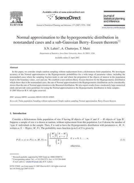
Normal approximation to the hypergeometric distribution in ...

Journal of Statistical Planning and Inference 137 (2007) 3570 – 3590
www.elsevier.com/locate/jspi
Normal approximation to the hypergeometric distribution in
nonstandard cases and a sub-Gaussian Berry–Esseen theorem
Abstract
S.N. Lahiri ∗ , A. Chatterjee, T. Maiti
Department of Statistics, Iowa State University, Ames, IA 50011, USA
Available online 21 April 2007
In this paper, we consider simple random sampling without replacement from a dichotomous finite population. We investigate
accuracy of the Normal approximation to the Hypergeometric probabilities for a wide range of parameter values, including the
nonstandard cases where the sampling fraction tends to one and where the proportion of the objects of interest in the population
tends to the boundary values, zero and one. We establish a non-uniform Berry–Esseen theorem for the Hypergeometric distribution
which shows that in the nonstandard cases, the rate of Normal approximation to the Hypergeometric distribution can be considerably
slower than the rate of Normal approximation to the Binomial distribution. We also report results from a moderately large numerical
study and provide some guidelines for using the Normal approximation to the Hypergeometric distribution in finite samples.
© 2007 Elsevier B.V. All rights reserved.
MSC: primary 60F05; secondary 60G10; 62E20; 62D05
Keywords: Finite population; Sampling without replacement; Simple random sampling; Normal approximation; Berry–Esseen theorem
1. Introduction
Consider a dichotomous finite population of size N having M objects of ‘type A’ and N − M objects of ‘type B’.
Suppose a sample of size n is drawn at random, without replacement from this population. Let X denote the number of
‘type A’-individuals in the sample. Then, X is said to have the Hypergeometric distribution with parameters n, M, N,
written as X ∼ Hyp(n; M,N). The probability mass function (p.m.f) of X is given by
⎧
M N − M
⎪⎨ x n − x
if x = 0, 1,...,n,
P(X= x) ≡ P(x; n, M, N) = N
(1.1)
⎪⎩ n
0 otherwise,
Research partially supported by NSF Grant no. DMS 0306574.
∗ Corresponding author. Tel.: +1 515 294 2271; fax: +1 515 294 4040.
E-mail address: snlahiri@iastate.edu (S.N. Lahiri).
0378-3758/$ - see front matter © 2007 Elsevier B.V. All rights reserved.
doi:10.1016/j.jspi.2007.03.033

Table 1
Error of Normal approximation
S.N. Lahiri et al. / Journal of Statistical Planning and Inference 137 (2007) 3570 –3590 3571
p f = 0.5 f = 0.6 f = 0.7 f = 0.8 f = 0.9
0.5 0.0562 0.0574 0.0613 0.0701 0.0929
0.6 0.0574 0.0593 0.0641 0.0743 0.0995
0.7 0.0613 0.0641 0.0702 0.0822 0.1112
0.8 0.0701 0.0743 0.0822 0.0972 0.1321
0.9 0.0929 0.0995 0.1112 0.1321 0.1787
Values of the absolute difference |P ((X−E(X))/Var(X)x)−(x)| at x=0 for different values of the parameters p and f, where X ∼ Hyp(n; M,N)
and (·) is the cdf of the N(0, 1) distribution. Here, N = 200 and M = Np and n = Nf .
where, for any two integers r 1 and s,
⎧
r ⎨ r!
if 0s r,
= s!(r − s)!
s ⎩
0 otherwise,
with 0! =1 and r! =1 · 2 ...r. Let f = n/N denote the sampling fraction and let p = M/N denote the proportion
of the ‘type A’-objects in the population. The Hypergeometric distribution plays an important role in many areas of
statistics, including sample surveys (Burstein, 1975; Wendell and Schmee, 1996), capture–recapture methods (Seber,
1970; Wittes, 1972), analysis of contingency tables (Blyth and Staudte, 1997), statistical quality control (von Collani,
1986; Patel and Samaranayake, 1991; Sohn, 1997), etc. Normal approximations to the Hypergeometric probabilities
P(.; n, M, N) of (1.1) are classical in the cases where the sampling fraction f and the proportion p are bounded away
from 0 and 1; for example, see Feller (1971). The nonstandard cases correspond to the extremes where f or p take values
near the boundary values 0 and 1. Although the nonstandard cases arise frequently in all these areas of applications,
the validity and accuracy of the normal approximation in such situations are not well studied. The quality of Normal
approximation deteriorates as the parameters f and p tend to their boundary values. For example, consider Table 1
where the cumulative distribution function (cdf) of the centered and scaled version (X − E(X))/ √ Var(X) of X at zero
is approximated by the Normal cdf at zero for different values of f and p.
Table 1 gives the values of the absolute difference of the cdfs of (X − E(X))/ √ Var(X) and the standard Normal
distribution at x =0. The population size is fixed at N =200 while the proportion p of ‘type A’-objects and the sampling
fraction f are varied over a range of 0.5–0.9 in increments of 0.1 (the values of p and f between 0 and 0.5 are omitted
due to the symmetry of the problem). In particular, for these choices of N and f, the sample size n = Nf takes the
values 100, 120, 140, 160 and 180. Note that even for such moderately large sample sizes, the error of approximation
increases steadily as p approaches the boundary value 1. Indeed, for p = 0.9 and f = 0.9, the error of approximation
is as high as 0.179 at the origin in the finite population sampling framework, which is significantly higher than 0.036,
the error of Normal approximation to the Binomial cdf with parameters n = 180 and p = 0.9. This shows that the
commonly known approximation results for the ‘with replacement sampling’ (or sampling from an infinite population)
case do not give a representative picture in the finite population setting when the parameters p and f are close to their
boundary values. For a better understanding, one needs to be able to quantify the accuracy of Normal approximation
as a function of N, p and f in the finite population setting.
In this paper, we derive a non-uniform Berry–Esseen theorem on Normal approximation to the Hypergeometric
distribution for a wide range of values of p and f, allowing these parameters go to the extreme points 0, 1. The nonuniform
bound in the Berry–Esseen theorem shows that the difference of the cdfs of (X − E(X))/ √ Var(X) and of a
standard Normal variate at a point x is bounded above by
g(x)[Nf (1 − f)p(1 − p)] −1/2 , (1.3)
where the function g(x) = g(x; p, f ) is bounded and decays at an exponential (sub-Gaussian) rate as a function of x.
As a corollary, we also derive an exponential (sub-Gaussian) probability inequality for the tails of X, which may be
of independent interest. Both the sub-Gaussian Berry–Esseen theorem and the exponential inequality seem to be new
even in the standard case.
(1.2)

3572 S.N. Lahiri et al. / Journal of Statistical Planning and Inference 137 (2007) 3570 – 3590
Note that the Hypergeometric variable X can be expressed as the sum of a collection of n dependent Bernoulli
random variables and (1.3) yields the uniform bound O([Np(1 − p)f (1 − f)] −1/2 ) on the error of Normal approximation
to the distribution of X. This rate is equivalent to the standard Berry–Esseen rate O(n −1/2 ) for the
Binomial distribution only when p is bounded away from 0 and 1 and f bounded away from 1. However, for p
and f close to these boundary points, the rate of approximation can be substantially slower. In such situations,
the dependence of the Bernoulli random variables associated with X has a nontrivial effect on the accuracy of the
Normal approximation. This provides the theoretical justification for the observed difference in the accuracy of
Normal approximations to the Binomial probabilities and to the Hypergeometric probabilities in the nonstandard
cases.
The theoretical findings of the paper and the numerical example in Table 1 also show that the existing guidelines for
applying the Normal approximation to the Binomial distribution (based on independent Bernoulli random variables)
are not appropriate for the Hypergeometric distribution in the nonstandard cases. To formulate a working guideline in
such situations, we conduct a moderately large numerical study and investigate the effect of the dependence in finite
samples. On the basis of the numerical study, in Section 3, we provide some ‘quick and easy’ guidelines for assessing
the error of Normal approximation to the Hypergeometric distribution in practice.
The rest of the paper is organized as follows. We conclude Section 1 with a brief literature review. Section 2
introduces the asymptotic framework and states the Berry–Esseen theorem and the exponential inequality. Results
from the numerical study are reported in Section 3. Proofs of all the results are given in Section 4.
For results on Normal approximations to Hypergeometric probabilities in the standard case where the sampling
fraction f and the proportion p are bounded away from 0 and 1, see Feller (1971). For general p and f, Nicholson (1956)
derived some very precise bounds for the point probabilities P(.; n, M, N) (cf. (1.1)) using some special normalizations
of the Hypergeometric random variable X. General methods for proving the central limit theorem (CLT) for sample
means under sampling without replacement from finite populations are given by Madow (1948), Erdos and Renyi
(1959), and Hajek (1960). In relation to the earlier work, the main contribution of our paper is to establish a nonuniform
Berry–Esseen theorem for the Hypergeometric distribution for a wide range of parameter values, including
the nonstandard case, and to provide some practical guidelines for using the Normal approximation in finite sample
applications.
2. Main results
Let r be a positive integer valued variable and for each r ∈ N (where N ={1, 2,...}), let Xr be a random variable
having the Hypergeometric distribution of (1.1) with parameters (nr,Mr,Nr), where nr,Mr,Nr ∈ N. Thus we consider
a sequence of dichotomous finite populations indexed by r, with the population of objects of type A and the sampling
fraction, respectively, given by
Let
pr = Mr
Nr
and fr = nr
Nr
for all r ∈ N. (2.1)
2 r ≡ Nrprqrfr(1 − fr), (2.2)
where qr = 1 − pr. Also, let (·) and (·), respectively, denote the density and the distribution function of a standard
Normal random variable, i.e., (x) = (1/ √ 2) exp(−x2 /2), x ∈ R and (x) = x
−∞ (t) dt, x ∈ R. Let I(·) denote
the indicator function. For x,y ∈ R, write x ∧ y = min{x,y}. Define
r = 1
10 (max(a1r, 2)) −1 , r1, (2.3)
where a1r = ( ¯
fr + 4)/4(1 − ¯
fr) and where ¯
fr = min{fr, 1 − fr}. Then, we have the following result.
Theorem 1. Suppose that Xr ∼ Hyp(nr,Mr,Nr), r ∈ N. Assume that r is such that:
rr > 1. (2.4)

S.N. Lahiri et al. / Journal of Statistical Planning and Inference 137 (2007) 3570 –3590 3573
Then there exists universal constants C1,C2 ∈ (0, ∞) (not depending on r, nr,Mr and Nr) such that:
P
Xr − nrpr
C1
x − (x)
1 +|x|
r
r
2
r(x) exp(−C2x 2 2 r (x)) (2.5)
for all x ∈ R, where r(x) = qrI(x0) + prI(x0).
Theorem 1 is a non-uniform Berry–Esseen theorem for the Hypergeometric distribution. It shows that the error of
Normal approximation to the Hypergeometric distribution dies at a sub-Gaussian rate in the tails. The only condition
needed for the validity of this bound is (2.4). It is easy to check that
r ∈ 1
25 , 1
20
(2.6)
for all r satisfying (2.4). Hence, the bound in (2.5) is available for all r such that r 25.
As pointed out in Section 1, when both the sequences {pr} {r 1} and {fr} {r 1} are bounded away from 0 and 1, the
rate of approximation in Theorem 1 matches the standard rate O(n −1/2
r ) of Normal approximation for the sum of nr
iid random variables with a finite third moment. Although the Hypergeometric random variable Xr can be written as
a sum of nr dependent Bernoulli (pr) variables, the lack of independence of the summands does not affect the rate of
Normal approximation as long as the sequence {pr} r 1 is bounded away from 0 and 1 and {fr} r 1 is bounded away
from 1. On the other hand, if either of the sequences {pr} {r 1} and {fr} {r 1} converge to one of the extreme values 0
and 1, then
r = o(n 1/2
r ) as r →∞
and the rate of Normal approximation to the Hypergeometric distribution is indeed worse than the standard rate O(n −1/2
r )
in such nonstandard cases.
An immediate consequence of Theorem 1 is the following exponential (sub-Gaussian) probability bound on the tails
of Xr.
Theorem 2. Suppose that Xr ∼ Hyp(nr,Mr,Nr), r ∈ N. Then, there exist universal constants C3,C4 ∈ (0, ∞) (not
depending on r, nr,Mr,Nr) such that for all r satisfying (2.4),
Xr − nrpr
P
x
C3
(pr ∧ qr) 3 exp(−C4x 2 [pr ∧ qr] 2 ) for all x>0.
r
3. Numerical results
To gain some insight into the quality of Normal approximation to the Hypergeometric distribution in finite samples
and to compare it with the accuracy in the case of the Binomial distribution, first we consider some joint plots of the
cdfs of normalized Hypergeometric and Binomial random variables against the standard Normal cdf. Figs. 1–5 show
these plots for different values of the parameters n and p for N = 60, 200.
From the figures, it follows that the quality of Normal approximation to the Hypergeometric distribution is comparable
to that for the Binomial distribution for values of f and p close to 0.5, but there is a stark loss of accuracy for high values
of f and p.
Next, to get a quantitative picture of the error of Normal approximation, we conducted a moderately large numerical
study with different values of the population size N and with different values of the parameters p and f. The population
sizes considered were N = 60, 200, 500, 2000. For a given value of N, the set of values of p and f considered was
{0.5, 0.6, 0.7, 0.8, 0.9}. We considered the Kolmogorov distance, i.e., the maximal distance between the cdfs of the
normalized Hypergeometric variable and a standard Normal variable as a measure of accuracy. More specifically, the
measure of accuracy for the Hypergeometric case is defined as
(N,p,f)=
P
X − np
x
− (x)
, (3.1)
where X ∼ Hyp(n, M, N), f = n/N, p = M/N, 2 = Nf (1 − f)p(1 − p) and (·) denotes the cdf of the N(0,1)
distribution.

3574 S.N. Lahiri et al. / Journal of Statistical Planning and Inference 137 (2007) 3570 – 3590
y (CDF)
1.0
0.8
0.6
0.4
0.2
0.0
Hypergeometric
Binomial
Normal
-5 0
x (Standardised)
Fig. 1. A plot of the cdfs of normalized Hypergeometric and Binomial random variables against the standard Normal cdf for the parameter values
N = 60, p = 0.5 and f = 0.5.
y (CDF)
1.0
0.8
0.6
0.4
0.2
0.0
Hypergeometric
Binomial
Normal
-15 -10 -5 0 5 10 15
x (Standardised)
Fig. 2. A plot of the cdfs of normalized Hypergeometric and Binomial random variables against the standard Normal cdf for the parameter values
N = 200, p = 0.5 and f = 0.5.
Tables 2–5 give the values of (N,p,f)for different combinations of the parameter values as indicated above. For
comparison, we also included the values of the maximal distance of the cdfs of normalized Binomial (n, p) and N(0,1)
random variables.
From Tables 2–5, it follows that the accuracy of the Normal approximation to the Hypergeometric distribution
deteriorates as p or f tend to the boundary value 1. Unlike the case of Normal approximation to the Binomial distribution,
the values of the sample size n and p alone are not a good indicator of the level of accuracy attainable in this case.
For example, for an iid sample of size n = 54 with p = 0.8, one may expect a reasonable accuracy of the Normal
5

y (CDF)
S.N. Lahiri et al. / Journal of Statistical Planning and Inference 137 (2007) 3570 –3590 3575
1.0
0.8
0.6
0.4
0.2
0.0
Hypergeometric
Binomial
Normal
-20 -15 -10 -5 0
x (Standardised)
Fig. 3. A plot of the cdfs of normalized Hypergeometric and Binomial random variables against the standard Normal cdf for the parameter values
N = 60, p = 0.9 and f = 0.7.
y (CDF)
1.0
0.8
0.6
0.4
0.2
0.0
Hypergeometric
Binomial
Normal
-20 -15 -10 -5 0
x (Standardised)
Fig. 4. A plot of the cdfs of normalized Hypergeometric and Binomial random variables against the standard Normal cdf for the parameter values
N = 60, p = 0.9 and f = 0.8.
approximation; the maximal error of approximation to the Binomial (54, 0.8) distribution is 0.0803. However, with
N = 60, n = 54 and p = 0.9, the maximal error of Normal approximation to the Hypergeometric distribution is as high
as 0.4633, making the approximation practically useless. With about a 9-fold increase in the sample size, at n = 450,
the accuracy of the approximation in the Hypergeometric case only improves to 0.1683 for the same values of f and p.
The corresponding maximal error for the Normal approximation to the Binomial distribution with parameters n = 450
and p = 0.8 is only 0.0282. Thus, the loss in accuracy in this case is an astounding 600% compared to the Binomial
5

3576 S.N. Lahiri et al. / Journal of Statistical Planning and Inference 137 (2007) 3570 – 3590
y (CDF)
1.0
0.8
0.6
0.4
0.2
0.0
Hypergeometric
Binomial
Normal
-20 -15 -10 -5 0
x (Standardised)
Fig. 5. A plot of the cdfs of normalized Hypergeometric and Binomial random variables against the standard Normal cdf for the parameter values
N = 60, p = 0.9 and f = 0.9.
Table 2
Values of the maximal error of Normal approximation to Hypergeometric distribution (viz., (N,p,f)of (3.1)) at N = 60 and the corresponding
values of the maximal error for the Binomial (n, p) distribution where n = Nf and p, f ∈{0.5, 0.6, 0.7, 0.8, 0.9}
Hypergeometric Binomial
n = 30 36 42 48 54 n = 30 36 42 48 54
p = 0.5 0.1017 0.1038 0.1106 0.1260 0.1646 0.0722 0.0660 0.0612 0.0573 0.0540
p = 0.6 0.1038 0.1066 0.1171 0.1284 0.1817 0.0785 0.0722 0.0661 0.0626 0.0588
p = 0.7 0.1106 0.1171 0.1283 0.1476 0.1844 0.0888 0.0808 0.0757 0.0711 0.0670
p = 0.8 0.2268 0.2528 0.2896 0.3480 0.4633 0.1070 0.0992 0.0922 0.0859 0.0803
p = 0.9 0.3128 0.3550 0.4046 0.4633 0.7169 0.1474 0.1391 0.1289 0.1184 0.1145
Table 3
Values of the maximal error of Normal approximation to Hypergeometric distribution (viz., (N,p,f)of (3.1)) at N = 200 and the corresponding
values of the maximal error for the Binomial (n, p) distribution where n = Nf and p, f ∈{0.5, 0.6, 0.7, 0.8, 0.9}
Hypergeometric Binomial
n = 100 120 140 160 180 n = 100 120 140 160 180
p = 0.5 0.0562 0.0574 0.0613 0.0701 0.0929 0.0398 0.0363 0.0337 0.0315 0.0297
p = 0.6 0.0574 0.0593 0.0641 0.0743 0.0995 0.0433 0.0395 0.0366 0.0343 0.0323
p = 0.7 0.0613 0.0641 0.0702 0.0822 0.1112 0.0491 0.0449 0.0416 0.0389 0.0367
p = 0.8 0.1261 0.1373 0.1559 0.1887 0.2634 0.0595 0.0543 0.0503 0.0471 0.0444
p = 0.9 0.1764 0.1922 0.2181 0.2634 0.3652 0.0832 0.0761 0.0705 0.0661 0.0623
case. Indeed, similar high levels of loss in accuracy occur for values of f and p near 1 even when the population size N
is increased to 2000 and beyond. As a consequence, the commonly used guidelines for the accuracy in the Binomial
case can be misleading for assessing accuracy of the Normal approximation to the Hypergeometric distribution in the
extreme cases.
5

S.N. Lahiri et al. / Journal of Statistical Planning and Inference 137 (2007) 3570 –3590 3577
Table 4
Values of the maximal error of Normal approximation to Hypergeometric distribution (viz., (N,p,f)of (3.1)) at N = 500 and the corresponding
values of the maximal error for the Binomial (n, p) distribution where n = Nf and p, f ∈{0.5, 0.6, 0.7, 0.8, 0.9}
Hypergeometric Binomial
n = 250 300 350 400 450 n = 250 300 350 400 450
p = 0.5 0.0356 0.0364 0.0389 0.0445 0.0592 0.0252 0.0230 0.0213 0.0199 0.0188
p = 0.6 0.0364 0.0376 0.0407 0.0472 0.0635 0.0274 0.0250 0.0232 0.0217 0.0205
p = 0.7 0.0389 0.0407 0.0446 0.0523 0.0712 0.0311 0.0284 0.0263 0.0246 0.0232
p = 0.8 0.0801 0.0872 0.0990 0.1200 0.1683 0.0378 0.0345 0.0319 0.0299 0.0282
p = 0.9 0.1124 0.1224 0.1390 0.1683 0.2355 0.0530 0.0484 0.0449 0.0420 0.0396
Table 5
Values of the maximal error of Normal approximation to Hypergeometric distribution (viz., (N,p,f)of (3.1)) at N = 2000 and the corresponding
values of the maximal error for the Binomial (n, p) distribution where n = Nf and p, f ∈{0.5, 0.6, 0.7, 0.8, 0.9}
Hypergeometric Binomial
n = 1000 1200 1400 1600 1800 n = 1000 1200 1400 1600 1800
p = 0.5 0.0178 0.0182 0.0195 0.0223 0.0297 0.0126 0.0115 0.0107 0.0010 0.0094
p = 0.6 0.0182 0.0188 0.0204 0.0237 0.0319 0.0137 0.0125 0.0116 0.0109 0.0102
p = 0.7 0.0195 0.0204 0.0224 0.0263 0.0358 0.0156 0.0142 0.0132 0.0123 0.0116
p = 0.8 0.0401 0.0437 0.0496 0.0602 0.0846 0.0189 0.0173 0.0160 0.0150 0.0141
p = 0.9 0.0564 0.0614 0.0698 0.0846 0.1189 0.0266 0.0243 0.0225 0.0210 0.0198
From Tables 2–5, it also follows that for a given value of N, if the parameter p is held fixed at a given level, the
maximal error of approximation to the Hypergeometric distribution increases monotonically as the value of f (i.e.,
n) increases, and vice versa. However, the sample size n and the value of p alone do not give a true indication of
the accuracy of the Normal approximation to the Hypergeometric distribution. To get a better estimate of the level of
accuracy, one must consider the combined effect of all three parameters N, f and p. Theorem 1 implies that the combined
effect of all three parameters on the maximal error of approximation can be expressed in terms of 1/(N,p,f), where
[(N,p,f)] 2 = Nfp(1 − p)(1 − f). To that effect, we define the co-efficient c(N, p, f ) ∈ (0, ∞) by the relation
Thus,
c(N, p, f ) = (N,p,f)(N,p,f). (3.2)
(N,p,f)≡ c(N, p, f )[(N,p,f)] −1 .
Using Theorem 1 and the lattice property of (X − E(X))/ √ Var(X), it can be shown that there exist two constants
C5,C6 ∈ (0, ∞) such that:
C5 c(N, p, f )C6
for all N,p,f, whenever (N,p,f)>0. If we knew the approximate value of C6 or of the co-efficient c(N, p, f ),
we could use C6[(N,p,f)] −1 or c(N, p, f )[(N,p,f)] −1 as a guideline for assessing the accuracy of Normal
approximation for the Hypergeometric distribution. Tables 6–9 below give the values of the co-efficient c(N, p, f ) for
different values of N,p,f.
Tables 6–9 show that the co-efficients c(N, p, f ) are surprisingly stable as a function of N, i.e., it exhibits very minor
variation as a function of N for a given value of the pair (p, f ). In a specific application with a given set of values of p
and f, one can use c(N, p, f )[(N,p,f)] −1 from Tables 6–9 to decide on the suitability of normal approximation to
the Hypergeometric probabilities.

3578 S.N. Lahiri et al. / Journal of Statistical Planning and Inference 137 (2007) 3570 – 3590
Table 6
Values of the co-efficients c(N, p, f ) at N = 60 for p, f ∈{0.5, 0.6, 0.7, 0.8, 0.9}
f = 0.5 0.6 0.7 0.8 0.9
p = 0.5 0.1970 0.1969 0.1964 0.1952 0.1913
p = 0.6 0.1969 0.1982 0.2036 0.1949 0.2069
p = 0.7 0.1964 0.2036 0.2086 0.2095 0.1963
p = 0.8 0.3513 0.3837 0.4112 0.4313 0.4306
p = 0.9 0.3634 0.4041 0.4308 0.4306 0.4998
Table 7
Values of the co-efficients c(N, p, f ) at N = 200 for p, f ∈{0.5, 0.6, 0.7, 0.8, 0.9}
f = 0.5 0.6 0.7 0.8 0.9
p = 0.5 0.1987 0.1987 0.1985 0.1982 0.1970
p = 0.6 0.1987 0.2012 0.2037 0.2058 0.2068
p = 0.7 0.1985 0.2037 0.2086 0.2132 0.2162
p = 0.8 0.3567 0.3806 0.4041 0.4269 0.4470
p = 0.9 0.3742 0.3994 0.4239 0.4470 0.46478
Table 8
Values of the co-efficients c(N, p, f ) at N = 500 for p, f ∈{0.5, 0.6, 0.7, 0.8, 0.9}
f = 0.5 0.6 0.7 0.8 0.9
p = 0.5 0.1992 0.1992 0.1991 0.1989 0.1985
p = 0.6 0.1992 0.2018 0.2043 0.2068 0.2088
p = 0.7 0.1991 0.2043 0.2095 0.2145 0.2189
p = 0.8 0.3581 0.3820 0.4058 0.4293 0.4517
p = 0.9 0.3771 0.4023 0.4273 0.4517 0.4740
Table 9
Values of the co-efficients c(N, p, f ) at N = 2000 for p, f ∈{0.5, 0.6, 0.7, 0.8, 0.9}
f = 0.5 0.6 0.7 0.8 0.9
p = 0.5 0.1994 0.1994 0.1994 0.1993 0.1992
p = 0.6 0.1994 0.2020 0.2047 0.2073 0.2098
p = 0.7 0.1994 0.2047 0.2010 0.2152 0.2203
p = 0.8 0.3588 0.3827 0.4066 0.4305 0.4540
p = 0.9 0.3785 0.4038 0.4290 0.4540 0.4785
4. Proofs
We now introduce some notation and notational convention to be used in this section. For real numbers x,y, let
x ∧ y = min{x,y} and x ∨ y = max{x,y}. Let ⌊x⌋ denote the largest integer not exceeding x, x ∈ R.Fora ∈ (0, ∞),
write a(x) = (1/a)(x/a) and a(x) = (x/a), x ∈ R, for the density and distribution functions of a N(0,a2 )
variable. Write a = and a = for a = 1. Let
∗
Xr − nrpr
r (x) = P
x − (x), x ∈ R. (4.1)
r
Let N ={1, 2,...}, Z+ ={0, 1,...} and Z ={...,−1, 0, 1,...}.

S.N. Lahiri et al. / Journal of Statistical Planning and Inference 137 (2007) 3570 –3590 3579
For notational simplicity, we shall drop the suffix r from notation, except when it is important to highlight the
dependence on r. Thus, we write n, M, N for nr,Mr,Nr, respectively, and set p = M/N, q = 1 − p and f = n/N.
We shall use C to denote a generic positive constant that does not depend on r. Unless otherwise stated, limits in order
symbols are taken by letting r →∞.
For proving the result, we shall frequently make use of Stirling’s approximation (cf. Feller, 1971)
m!= √ 2e −m+m m m+1/2
where the error term m admits the bound
1
12m + 1 m 1
12m
for all m ∈ N, (4.2)
for all m ∈ N.
Also note that for g(y) = log y, y ∈ (0, ∞), the kth derivative of g is given by g (k) (y) = ((−1) k−1 (k − 1)!)/y k ,
y ∈ (0, ∞), k ∈ N. Hence, for any k ∈ N and ∈ (0, 1),
|g (k) (k − 1)!
(1 + x) |
(1 − ) k
for all 0|x| < . (4.3)
For Lemma 1 below, let X ∼ Hyp(n; M,N) for a given set of integers n, M, N ∈ N with 1n(N − 1),
1M (N − 1). Let
xk,n =
k − np
√ npq
and ak,n =
xk,n
(1 − f) √ , 0k n, (4.4)
npq
where f = n/N, p = M/N and q = 1 − p. Lemma 1 gives a basic approximation to Hypergeometric probabilities
solely under condition (4.5) stated below.
Lemma 1. Suppose that X ∼ Hyp(n; M,N) for a given set of integers n, M, N ∈ N such that
0

3580 S.N. Lahiri et al. / Journal of Statistical Planning and Inference 137 (2007) 3570 – 3590
First consider R(k; n, M, N). By (4.2),
n−1
j=1
k−1
j=1
1 − j
=
N
1 − j
Np
Note that by (4.4),
Next write
and
k
= f + xk,n
Np
zk,n = xk,n
e (−N+N ) N N+1/2
e (−(N−n)+N−n) (N − n) N−n+1/2
= e(N −N−n) e−n ,
N(1−f)+1/2 (1 − f)
n−k−1
j=1
fq
Np
√ fp/Nq
1 − f
1 − j
=
Nq
and
n − k
Nq
, yk,n = xk,n
√
fq/Np
1 − f
1
N n
e −n e Np−Np−k+Nq−Nq−n+k
(1 − k/Np) Np−k+1/2 .
Nq−n+k+1/2 (1 − (n − k)/Nq)
= f − xk,n
fp
.
Nq
(4.9)
∗ = Np − Np−k + Nq − Nq−n+k + N−n − N . (4.10)
Then R(k; n, M, N) can be expressed as
log R(k; n, M, N) = ∗ −
log(1 − f)
2
− Nq(1 − f)(1 + zk,n) + 1
2
≡ ∗ −
log(1 − f)
2
Fix ∈ (0, 1 2 ). By Taylor’s expansion and (4.3),
A1 = Np(1 − f)(1− yk,n) + 1
log(1 − yk,n)
2
= Np(1 − f)(1− yk,n) + 1
2
− Np(1 − f)(1− yk,n) + 1
log(1 − yk,n)
log(1 + zk,n)
2
− A1 − A2 say. (4.11)
−yk,n − y2 k,n
2
+ r1n(k)
=−yk,n Np(1 − f)+ 1
−
2
y2
k,n 1
− Np(1 − f) + r2n(k), (4.12)
2 2
where r1n(k) and r2n(k) are remainder terms, defined by the equality of the successive expressions. By (4.3), for all
n, k satisfying |yk,n|,
and
2
|r1n(k)|
(1 − ) 3
|yk,n| 3
3!
|r2n(k)| Np
2 (1 − f)|yk,n| 3
+
Np(1 − f)(1− yk,n) + 1
2 ·|r1n(k)|. (4.13)

S.N. Lahiri et al. / Journal of Statistical Planning and Inference 137 (2007) 3570 –3590 3581
By similar arguments,
A2 = Nq(1 − f)(1 + zk,n) + 1
log(1 + zk,n)
2
=
Nq(1 − f)+ 1
zk,n +
2
z2 k,n
2
where for all n, k, satisfying |zk,n|,
|zk,n|
3
|r3n(k)|Nq(1 − f)
2 +
Nq(1 − f)(1 + zk,n) + 1
2 ·
From, (4.11), (4.12) and (4.14), we have
(zk,n − yk,n)
log R(k; n, M, N) = ∗ −
+ y2 k,n
2
log(1 − f)
2
Nq(1 − f)− 1
+ r3n(k), (4.14)
2
−
2
+ z2 k,n
2
|zk,n| 3
Np(1 − f)− 1
+ r2n(k) + r3n(k)
2
. (4.15)
3 3(1 − )
Nq(1 − f)− 1
2
= ∗ − 1
2 log(1 − f)− x2 k,nf 2(1 − f) + r4n(k), (4.16)
where for all n, k satisfying (|yk,n|∨|zk,n|),
|r4n(k)||r2n(k)|+|r3n(k)|+ 1 2 |yk,n − zk,n|+ 1 4 (y2 k,n + z2 k,n ).
Next using Stirling’s formula on the binomial term, we have
n
log p
k
k q n−k
e
= log
(n−k−n−k)
√ 1
p
√ − nq − xk,n npq + log 1 − xk,n
2npq
2
nq
√ 1
q
− np + xk,n npq + log 1 + xk,n
2
np
≡ ∗∗ − log 2npq − A3 − A4 say, (4.17)
where ∗∗ √ √
= n − k − n−k. Next write ˜yk,n = xk,n p/nq and ˜zk,n = xk,n q/np. Then, by arguments similar to (4.12)
and (4.14),
√ 1
p
A3 = nq − xk,n npq + log 1 − xk,n
2
nq
=−˜yk,n nq + 1
+
2
˜y2
k,n
nq −
2
1
+ r5n(k)
2
and
√ 1
q
A4 = np + xk,n npq + log 1 + xk,n
2
np
=˜zk,n np + 1
+
2
˜z2
k,n
np −
2
1
+ r6n(k),
2

3582 S.N. Lahiri et al. / Journal of Statistical Planning and Inference 137 (2007) 3570 – 3590
where for all k and n satisfying (|˜yk,n|∨|˜zk,n|),
|r5n(k)|+|r6n(k)| n
2 [q|˜yk,n| 3 + p|˜zk,n| 3 2
]+
(1 − ) 3
nq + 1
+ nq|˜yk,n| |˜yk,n|
2 3
+ np + 1
+ np|˜zk,n| |˜zk,n|
2 3
. (4.18)
Hence, as in (4.16), it follows that
n
log p
k
k q n−k
= ∗∗ − log 2npq − 1
2 x2 k,n + r7n(k), (4.19)
where for all n, k satisfying (|˜yk,n|∨|˜zk,n|),
Note that
|r7n(k)|| 1 2 (˜zk,n +˜yk,n) − 1 4 ( ˜y2 k,n +˜z2 k,n )|+|r5n(k)|+|r6n(k)|.
fq + fp + (1 − f)p+ (1 − f)q= 1,
(fq) 2 + (fp) 2 + ((1 − f)p) 2 + ((1 − f)q) 2 = (1 − 2pq)(1 − 2(1 − f))

Note that for all k, n satisfying |ak,n|,
S.N. Lahiri et al. / Journal of Statistical Planning and Inference 137 (2007) 3570 –3590 3583
(1 − f)
Np − k Np − (np + (1 − f)npq)>np > 0
2
and
(1 − f)
Nq − (n − k)>nq > 0.
2
Hence, by the error bound in Stirling’s approximation, for all k, n with |ak,n| and 6(np ∧ nq)1,
∗ 1
12Np + 1 −
1
12(Np − k) +
1
12Nq + 1 −
1
12(Nq − (n − k)) +
1 1
−
12(N − n) + 1 12N
−
−
12k + 1
(12Np + 1)(12(Np − k)) −
12(n − k) + 1
(12Nq + 1)(12(Nq − n + k))
1
6Np(1 − )(1 − f) −
1
6Nq(1 − )(1 − f)
f
=−
6npq(1 − )(1 − f) ,
∗
1 1
f
0 + 0 +
−
12(N − n) + 1 12N 6npq(1 − )(1 − f) ,
∗∗ 1
12n −
1
12k + 1 −
1
12(n − k) + 1 0,
∗∗ 1 1
−
12n + 1 12k −
1
n
1
−
−
12(n − k) 12k(n − k) 6npq(1 − ) .
Hence, the lemma follows from (4.21) and the above inequalities.
Lemma 2. Let g : R −→ [0, ∞) be such that g is ↑ on (−∞,a)andgis↓ on (a, ∞) for some a ∈ R. Then, for any
k ∈ N, b ∈ R and h ∈ (0, ∞),
k
g(b + ih)
i=o
b+hk
where g(x0) = max{g(b + ih) : i = 0, 1,...,k}.
Proof. For ba, by monotonicity,
h
k
g(b + ih)hg(b) +
i=0
b
g(x)dx + 2hg(x0), (4.22)
b+hk
b
g(x)dx.
For b

3584 S.N. Lahiri et al. / Journal of Statistical Planning and Inference 137 (2007) 3570 – 3590
Hence, for bk1,
h
k
k1
g(b + ih) = h g(b + ih) + h
i=0
i=0
i=0
k
i=k1+1
j=0
g(b + ih)
k1
k−k1−1
= h g(b + ih) + h g(b1 + h + jh)
b1
b
b+hk
b
g(x)dx + hg(b1) + hg(b1 + h) +
g(x)dx + 2hg(x0).
b1+h+(k−k1−1)h
b1+h
g(x)dx − hg(b1)
For b

S.N. Lahiri et al. / Journal of Statistical Planning and Inference 137 (2007) 3570 –3590 3585
Next consider the case where 0 ∈[b− h/2,b+ h/2). Then, by Taylor’s expansion,
b−h/2
h(b) − (x) dx
h3 | ′′ (0)|/24.
b−h/2
Now using similar arguments for the case ‘ √ 3 ∈ (b − h/2,b + (j0 + 1 2 )h)’ and using the above bounds, one can
complete the proof of the lemma.
Proof of Theorem 1. Let r ∈ N be an integer such that (2.4) holds. Since r will be held fixed all through the proof,
we shall drop r from the notation for simplicity, and write fr = f , r = , pr = p, qr = q, nr − n, etc. First, suppose
that f 1 2 . Consider the case x 0. Let ˜xk = xk/ √ 1 − f = (k − np)/, k = 0, 1,...,n. Define
and
K0 = sup{k ∈ Z+ :˜xk 0},
K1 = inf{k ∈ Z+ :˜xk − 1},
K2 = inf{k ∈ Z+ :˜xk − }
Jx =⌊np + x⌋, x ∈ R,
where ≡ r ∈ (0, 1 2 ] is as in (2.3). Note that by definition,
K1 − 1

3586 S.N. Lahiri et al. / Journal of Statistical Planning and Inference 137 (2007) 3570 – 3590
Now, from (4.25), for all K2 j

S.N. Lahiri et al. / Journal of Statistical Planning and Inference 137 (2007) 3570 –3590 3587
Hence, for −1x 0, noting that K0 − K1 ,
|1(x)|
K0
j=K1
exp(−˜x 2 j (0.07)) exp(−1 ) 5a1
√ 2 2
(K0 − K1) exp( −1 ) 5a1
√ 2 2
C
. (4.29)
Thus, the bound (4.28) on I2 holds for all x ∈[−, 0].
Next consider I1. Note that for j ∈{0, 1,...,n},
P(X= j + 1)P(X= j)
Np − j
⇔
j + 1 .
n − j
Nq − n + j + 1 1
n(Np + 1) Nq + 1
⇔ j − . (4.30)
N + 2 N + 2
Thus, P(X= j)

3588 S.N. Lahiri et al. / Journal of Statistical Planning and Inference 137 (2007) 3570 – 3590
Since ˜xJx x and ˜xK2 − + −1 , by Lemma 3, for x ∈[−, 0], one gets
Jx
I3
1
˜xJx
( ˜xj ) −
j=K2
+(2)−1
˜xK 2 −(2) −1
(y) dy
+|(x) − ( ˜xJx + (2)−1 )|+( ˜xK2 − (2)−1 )
1
122 x+1/2
|
−∞
′′
(y)| dy + 5 max | ′′ (y)| :−∞

S.N. Lahiri et al. / Journal of Statistical Planning and Inference 137 (2007) 3570 –3590 3589
Next note that
X − np
P
x
= 0 for all x 1. This proves (2.5) for x ∈ (−∞, 0] and f 1 2 . To prove the theorem for x 0 and f 1 2 , define
Vr = nr − Xr, r ∈ N.
Note that Vr has a Hypergeometric distribution with parameters (nr,Nr − Mr,Nr). Further,
Xr − nrpr
r
=− Vr − nrqr
r
for all r ∈ N.
Hence, the derived bound on the right tails of (Xr − nrpr)/r, can be obtained by repeating the arguments above with
Xr replaced by Vr and pr replaced by qr for any r such that r > 1. This proves (2.5) for x ∈[0, ∞) and f 1 2 .
Next suppose that fr > 1 2 . Consider the collection of Nr − nr objects that are left after the sample of size nr has been
selected from the population of size Nr. Let Yr is the number of ‘type A’-objects in this collection. Then, for all r ∈ N
and j ∈ Z,
Hence,
Yr ∼ Hyp(Nr − nr; Mr,Nr) and P(Xr = j)= P(Yr = Mr − j). (4.34)
P(Xr k) =
k
P(Xr = j)=
j=0
k
P(Yr = Mr − j)= P(YrMr − k).
j=0
Further, note that Var(Yr) = (Nr − nr)prqr(1 − (Nr − nr)/Nr) = 2 r . Hence, for each x ∈ R,
Xr − nrpr
P
x = P (Xr nrpr + xr)
r
= P(Xr⌊nrpr + xr⌋)
= P(YrMr −⌊nrpr + xr⌋)
= P(˜Yr ˇxr) (say),

3590 S.N. Lahiri et al. / Journal of Statistical Planning and Inference 137 (2007) 3570 – 3590
where ˜Yr = (Yr − (Nr − nr)pr)/r and ˇxr = (Mr −⌊nrpr + xr⌋−(Nr − nr)pr)/r. Note that,
ˇxr < 1
[Nrpr − (nrpr + xr − 1) − Nrpr + nrpr] =−x + −1
r
r
and similarly, ˇxr − x. Hence, this implies,
and
P(˜Yr < ˇxr)P(˜Yr ˇxr)P(˜Yr − x + −1
r )
P(˜Yr < ˇxr)P(˜Yr < − x)P(˜Yr − x − −1
r ).
Now using the above identity and inequalities, we have
P
Xr − nrpr
x − (x)
=|P(˜Yr ˇxr) − (1 − (−x))|
r
=|(−x) − P(˜Yr < ˇxr)|
max{|P(˜Yr − x − −1
r ) − (−x − −1 r )|,
|P(˜Yr − x + −1
r ) − (−x + −1 r )|}
+ max{|(−x) − (−x − −1
r )|, |(−x) − (−x + −1 r )|}. (4.35)
The proof of (2.5) for ‘f ∈[ 1 2 , 1] and x ∈ R’ follows by replacing the above arguments with Xr,fr replaced by
Yr, 1 − fr, respectively, and using the bound (4.34) and (4.35). This completes the proof of the theorem.
Proof of Theorem 2. Use (2.5) and the inequality ‘exp(x)(1 + x) for all x ∈ (0, ∞)’.
References
Blyth, C.R., Staudte, R.G., 1997. Hypothesis estimates and acceptability profiles for 2 × 2 contingency tables. J. Amer. Statist. Assoc. 92, 694–699.
Burstein, H., 1975. Finite population correction for binomial confidence limits. J. Amer. Statist. Assoc. 70, 67–69.
Erdos, P., Renyi, A., 1959. On the central limit theorem for samples from a finite population. Magyar Tudoanyos Akademia Budapest Matematikai
Kutato Intezet Koezlemenyei. Trudy Publications, vol. 4, pp. 49–57.
Feller, W., 1971. An Introduction to Probability Theory and its Applications, vol. I. Wiley, New York, NY.
Hajek, J., 1960. Limiting distributions in simple random sampling from a finite population. Magyar Tudoanyos Akademia Budapest Matematikai
Kutato Intezet Koezlemenyei. Trudy Publications, vol. 5, pp. 361–374.
Nicholson, W.L., 1956. On the normal approximation to the hypergeometric distribution. Ann. Math. Statist. 27, 471–483.
Madow, W.G., 1948. On the limiting distributions of estimates based on samples from finite universes. Ann. Math. Statist. 19, 535–545.
Patel, J.K., Samaranayake, V.A., 1991. Predictions intervals for some discrete distributions. J. Qual. Technol. 23, 270–278.
Seber, G.A.F., 1970. The effects of trap response on tag recapture estimates. Biometrics 26, 13–22.
Sohn, S.Y., 1997. Accelerated life-tests for intermittent destructive inspection, with logistic failure-distribution. IEEE Trans. Reliab. 46, 122–1295.
von Collani, E., 1986. The -optimal acceptance sampling scheme. J. Qual. Technol. 18, 63–66.
Wendell, J.P., Schmee, J., 1996. Exact inference for proportions from a stratified finite population. J. Amer. Statist. Assoc. 91, 825–830.
Wittes, J.T., 1972. On the bias and estimated variance of Chapman’s two-sample capture-recapture population estimate. Biometrics 28, 592–597.