

Linear Transformation Examples Matrix Eigenvalue problems
Linear Transformation Examples Matrix Eigenvalue problems
Linear Transformation Examples Matrix Eigenvalue problems

You also want an ePaper? Increase the reach of your titles
YUMPU automatically turns print PDFs into web optimized ePapers that Google loves.
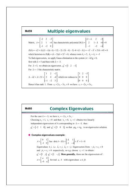
Md59<br />
Multiple eigenvalues<br />
⎡−2<br />
2 −3⎤<br />
−2−λ2 −3<br />
<strong>Matrix</strong>, A= ⎢<br />
2 1 −6<br />
⎥<br />
has characteristic polyomial D(<br />
λ)<br />
= 2 1−λ−6 = 0<br />
⎢<br />
⎥<br />
⎣⎢<br />
−1 −2<br />
0 ⎦⎥<br />
−1 −2 −λ<br />
3 2<br />
D(<br />
λ) =− ( 2+ λ){( 1−λ)( −λ) −12} −2{ −2λ −6} −3{ − 4+ ( 1− λ)} =−λ − λ + 21λ + 45 = 0<br />
2<br />
which factorises to D(<br />
λλ) = ( λ − 5)( λ + 3) = 0, whence roots λ1 = 5, λ2 = λ3<br />
= −3<br />
To find eigenvectors, we apply Gauss elimination to the system ( A− λI)<br />
x = 0,<br />
first with λ = 5 and then with λ = −3.<br />
T<br />
For λ = 5, we obtain an eigenvector, e1<br />
= [ 1 2 −1]<br />
For λ =−3<br />
the characteristic matrix<br />
⎡ 1<br />
A − λI<br />
= A+ 3I<br />
=<br />
⎢<br />
2<br />
⎢<br />
⎣⎢<br />
−1 2<br />
4<br />
−2<br />
−3⎤<br />
−6<br />
⎥<br />
⎥<br />
3 ⎥⎦<br />
⎡1<br />
which row reduces to<br />
⎢<br />
0<br />
⎢<br />
⎣⎢<br />
0<br />
2<br />
0<br />
0<br />
−3⎤<br />
0<br />
⎥<br />
⎥<br />
0 ⎦⎥<br />
Hence it has rank 1. From x + 2x − 3x = 0 we have x = − 2x + 3x<br />
.<br />
Md60<br />
1 2 3 1 2 3<br />
Complex <strong>Eigenvalue</strong>s<br />
For the case λ =− 3, we have x1<br />
=− 2x2 + 3x3<br />
:<br />
Choosing x2 = 1, x3 = 0 and then x2 = 0, x3<br />
= 1 obtains two linearly<br />
independent eigenvectors of A corresponding to λ =−3,<br />
thus :<br />
T T<br />
e = −2<br />
1 0 , and e 3 0 1;<br />
so that µ e νe<br />
is an eigenvector solution.<br />
[ ] = [ ] +<br />
2 3 2 3<br />
● Complex eigenvalues example:<br />
⎡<br />
A= ⎢<br />
⎣−<br />
⎤<br />
⎥<br />
⎦<br />
A− I =<br />
j ie j j jx x<br />
jx x x<br />
T<br />
e<br />
T<br />
j e j<br />
−<br />
0<br />
1<br />
1<br />
0<br />
λ<br />
has det( λ )<br />
−1 1 2<br />
= λ + 1= 0<br />
− λ<br />
<strong>Eigenvalue</strong>s ± , . . λ1 = , λ2<br />
= − ; Eigenvectors from − 1 + 2 = 0<br />
and 1 + 2 = 0 respectively, so e.g. choose 1 = 1 to obtain :<br />
1 = [ 1 ] , 2 = [ 1 − ] . More generally, these are the eigenvectors of :<br />
⎡ a<br />
A = ⎢<br />
⎣−b<br />
b⎤<br />
for real a b with eigenvalues a jb<br />
a⎥<br />
, , ± .<br />
⎦