

Linear Transformation Examples Matrix Eigenvalue problems
Linear Transformation Examples Matrix Eigenvalue problems
Linear Transformation Examples Matrix Eigenvalue problems

Create successful ePaper yourself
Turn your PDF publications into a flip-book with our unique Google optimized e-Paper software.
Md53<br />
<strong>Linear</strong> <strong>Transformation</strong> <strong>Examples</strong><br />
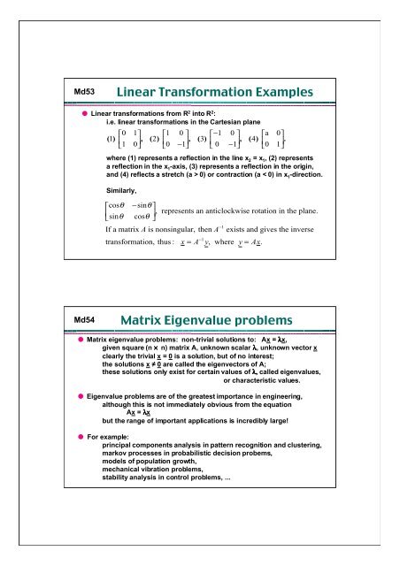
● <strong>Linear</strong> transformations from R2 into R2 :<br />
i.e. linear transformations in the Cartesian plane<br />
⎡0<br />
1⎤<br />
⎡1<br />
0 ⎤ ⎡−1<br />
0 ⎤ ⎡a<br />
0⎤<br />
() 1 ⎢ , ( 2)<br />
, ( 3)<br />
, ( 4)<br />
.<br />
⎣1<br />
0⎥<br />
⎢<br />
⎦ ⎣0<br />
−1⎥<br />
⎢<br />
⎦ ⎣ 0 −1⎥<br />
⎢<br />
⎦ ⎣0<br />
1⎥<br />
⎦<br />
Md54<br />
where (1) represents a reflection in the line x 2 = x 1, (2) represents<br />
a reflection in the x 1-axis, (3) represents a reflection in the origin,<br />
and (4) reflects a stretch (a > 0) or contraction (a < 0) in x 1-direction.<br />
Similarly,<br />
⎡cosθ<br />
−sinθ⎤<br />
⎢<br />
,<br />
⎣sinθ<br />
cosθ<br />
⎥ represents an anticlockwise rotation in the plane.<br />
⎦<br />
−1<br />
If a matrix Ais nonsingular, then A exists and gives the inverse<br />
−1<br />
transformation, thus : x = A y, where y = Ax.<br />
<strong>Matrix</strong> <strong>Eigenvalue</strong> <strong>problems</strong><br />
● <strong>Matrix</strong> eigenvalue <strong>problems</strong>: non-trivial solutions to: Ax = λx,<br />
given square (n ×× n) matrix A, unknown scalar λ, unknown vector x<br />
clearly the trivial x = 0 is a solution, but of no interest;<br />
the solutions x ≠ 0 are called the eigenvectors of A;<br />
these solutions only exist for certain values of λ, called eigenvalues,<br />
or characteristic values.<br />
● <strong>Eigenvalue</strong> <strong>problems</strong> are of the greatest importance in engineering,<br />
although this is not immediately obvious from the equation<br />
Ax = λλx<br />
but the range of important applications is incredibly large!<br />
● For example:<br />
principal components analysis in pattern recognition and clustering,<br />
markov processes in probabilistic decision probems,<br />
models of population growth,<br />
mechanical vibration <strong>problems</strong>,<br />
stability analysis in control <strong>problems</strong>, ...
Md55<br />
<strong>Eigenvalue</strong>s and Eigenvectors<br />
● Terminology:<br />
Ax = λx matrix eigenvalue problem<br />
A value of λλ for which x (≠ 0) is a solution eigenvalue,<br />
(also known as characteristic value)<br />
Solutions x (≠ 0) corresponding to a λ called eigenvectors<br />
The set of eigenvectors is called the spectrum of A<br />
Largest of absolute values of eigenvalues is spectral radius of A<br />
● Determination of eigenvalues and eigenvectors:<br />
Ax = λx = λIx, where I is the identity matrix<br />
(A - λI)x = 0, homogeneous linear system with non-trivial solution<br />
(x ≠ 0) if and only if D(λλ) = det(A - λI) = 0<br />
Md56<br />
Example<br />
Ax = x A =<br />
x<br />
x<br />
x<br />
x x x<br />
x x x<br />
− ⎡<br />
⎢<br />
⎣<br />
⎤<br />
− ⎥ =<br />
⎦<br />
⎡<br />
● Determination of eigenvalues :<br />
5<br />
λ ,<br />
2<br />
2<br />
1 ⎤<br />
, ⎢ ⎥,<br />
so that<br />
2 ⎣ 2 ⎦<br />
− 5 1 + 2 2 = λ 1<br />
2 1 − 2 2 = λ 2<br />
− − x + x =<br />
A− I x =<br />
x + − − x =<br />
D = A− I = −<br />
( 5 λ)<br />
1 2 2 0<br />
( λ ) 0,<br />
2 1 ( 2 λ)<br />
2 0<br />
and<br />
5−λ ( λ) det( λ )<br />
2<br />
2<br />
= 0<br />
−2−λ Characteristic polynomial<br />
2<br />
D(<br />
λ) = ( −5−λ)( −2−λ) − 4 = λ + 7λ + 6= 0<br />
Whence, ( λ + 1)( λ + 6) = 0, so that λ = −1, − 6; i.e. λ =− 1, λ =−6.<br />
● Determination of an eigenvector:<br />
1 2<br />
For<br />
− + =<br />
λ = λ = − :<br />
− =<br />
and these equations are linearly dependent<br />
with a solution : = . This determines an eigenvector corresponding to λ = −<br />
up to a scalar multiple. If we choose x 1 = , we obtain eigenvector x = e1<br />
= .<br />
⎡ ⎤ ⎡<br />
⎢ ⎥ = ⎢<br />
⎣ ⎦ ⎣<br />
⎤<br />
4x1 2x2 0<br />
1 1<br />
2x1 x2<br />
0<br />
x2 2x1 1 1<br />
x1<br />
1<br />
1<br />
x ⎥<br />
2 2⎦
Md57<br />
General Case<br />
● Determination of other eigenvector:<br />
+ =<br />
For λ = λ = − :<br />
and these equations are linearly dependent<br />
+ =<br />
with a solution : =− / with arbitrary . This determines an eigenvector<br />
corresponding to λ =− up to a scalar multiple. If we choose x 1 = , we obtain<br />
eigenvector x = e2 = . So that : λ , e1<br />
⎡ ⎤<br />
⎢ ⎥<br />
⎣ ⎦<br />
= ⎡ ⎤<br />
⎢<br />
⎣−<br />
⎥ =− =<br />
⎦<br />
⎡<br />
x1 2x2 0<br />
2 6<br />
2x1 4x2 0<br />
x2 x1 2<br />
x1<br />
2 6 2<br />
x1<br />
2<br />
1<br />
1 1<br />
x2<br />
1<br />
⎢<br />
⎣2<br />
⎤<br />
⎡ 2 ⎤<br />
⎥ ; λ2 =− 6,<br />
e2 = ⎢<br />
⎦<br />
⎣−<br />
⎥.<br />
1⎦<br />
● <strong>Eigenvalue</strong>s:<br />
The eigenvalues of a square matrix A are the roots of the characteristic<br />
equation D(λ) = det(A - λI) = 0. Hence an n × n matrix has at least one<br />
eigenvalue and at most n numerically different eigenvalues.<br />
● Eigenvectors:<br />
If x is an eigenvector of a matrix A corresponding to an eigenvalue λλ, so<br />
is kx with any k ≠ 0. [since Ax = λx implies k(Ax) = λ(kx)].<br />
Md58<br />
Characteristic Polynomial<br />
For n× n matrix A, Ax = λx, whence ( A− λI)<br />
x = 0,<br />
This homogeneous linear system<br />
of equations has a nontrivial solution if and only if D( λ) = det( A− λI)<br />
= 0 :<br />
a11 − λ a12 ... a1n<br />
D( λ) = det( A− λI)<br />
=<br />
a21 .<br />
a22 − λ<br />
.<br />
...<br />
...<br />
a2n<br />
.<br />
= 0<br />
a a ... a − λ<br />
n1 n2 nn<br />
which develops a polynomial of nth degree in λ,<br />
called the characteristic polynomial of A :<br />
n<br />
n−1<br />
D(<br />
λ) = λ + bn−1λ + . . . + b1λ + b0<br />
= 0,<br />
which has at least one root<br />
(solution for eigenvalue λ), and at most n numerically different roots, λ.<br />
n<br />
e.g. ( λ − λ0) = 0,<br />
whence λ = λ0<br />
or ( λ −λ1)( λ −λ2) . . . ( λ − λn) = 0, whence λ = λi,<br />
i = 1,<br />
. . . , n<br />
Note that the roots can be real or complex, but if matrix A has real coefficients,<br />
then any complex roots occur in complex conjugate pairs, e.g. λ = c+ jd λ = c− jd<br />
k , k+<br />
1
Md59<br />
Multiple eigenvalues<br />
⎡−2<br />
2 −3⎤<br />
−2−λ2 −3<br />
<strong>Matrix</strong>, A= ⎢<br />
2 1 −6<br />
⎥<br />
has characteristic polyomial D(<br />
λ)<br />
= 2 1−λ−6 = 0<br />
⎢<br />
⎥<br />
⎣⎢<br />
−1 −2<br />
0 ⎦⎥<br />
−1 −2 −λ<br />
3 2<br />
D(<br />
λ) =− ( 2+ λ){( 1−λ)( −λ) −12} −2{ −2λ −6} −3{ − 4+ ( 1− λ)} =−λ − λ + 21λ + 45 = 0<br />
2<br />
which factorises to D(<br />
λλ) = ( λ − 5)( λ + 3) = 0, whence roots λ1 = 5, λ2 = λ3<br />
= −3<br />
To find eigenvectors, we apply Gauss elimination to the system ( A− λI)<br />
x = 0,<br />
first with λ = 5 and then with λ = −3.<br />
T<br />
For λ = 5, we obtain an eigenvector, e1<br />
= [ 1 2 −1]<br />
For λ =−3<br />
the characteristic matrix<br />
⎡ 1<br />
A − λI<br />
= A+ 3I<br />
=<br />
⎢<br />
2<br />
⎢<br />
⎣⎢<br />
−1 2<br />
4<br />
−2<br />
−3⎤<br />
−6<br />
⎥<br />
⎥<br />
3 ⎥⎦<br />
⎡1<br />
which row reduces to<br />
⎢<br />
0<br />
⎢<br />
⎣⎢<br />
0<br />
2<br />
0<br />
0<br />
−3⎤<br />
0<br />
⎥<br />
⎥<br />
0 ⎦⎥<br />
Hence it has rank 1. From x + 2x − 3x = 0 we have x = − 2x + 3x<br />
.<br />
Md60<br />
1 2 3 1 2 3<br />
Complex <strong>Eigenvalue</strong>s<br />
For the case λ =− 3, we have x1<br />
=− 2x2 + 3x3<br />
:<br />
Choosing x2 = 1, x3 = 0 and then x2 = 0, x3<br />
= 1 obtains two linearly<br />
independent eigenvectors of A corresponding to λ =−3,<br />
thus :<br />
T T<br />
e = −2<br />
1 0 , and e 3 0 1;<br />
so that µ e νe<br />
is an eigenvector solution.<br />
[ ] = [ ] +<br />
2 3 2 3<br />
● Complex eigenvalues example:<br />
⎡<br />
A= ⎢<br />
⎣−<br />
⎤<br />
⎥<br />
⎦<br />
A− I =<br />
j ie j j jx x<br />
jx x x<br />
T<br />
e<br />
T<br />
j e j<br />
−<br />
0<br />
1<br />
1<br />
0<br />
λ<br />
has det( λ )<br />
−1 1 2<br />
= λ + 1= 0<br />
− λ<br />
<strong>Eigenvalue</strong>s ± , . . λ1 = , λ2<br />
= − ; Eigenvectors from − 1 + 2 = 0<br />
and 1 + 2 = 0 respectively, so e.g. choose 1 = 1 to obtain :<br />
1 = [ 1 ] , 2 = [ 1 − ] . More generally, these are the eigenvectors of :<br />
⎡ a<br />
A = ⎢<br />
⎣−b<br />
b⎤<br />
for real a b with eigenvalues a jb<br />
a⎥<br />
, , ± .<br />
⎦
Md61<br />
Stretching elastic membrane<br />
2 2<br />
Elastic membrane in xx 1 2 − plane with boundary circle x1 + x2<br />
= 1<br />
is stretched so that point P x1 x2 goes over into point Q y1 y2<br />
by :<br />
y1<br />
5 3 x1<br />
y = Ax<br />
y2<br />
3 5 x2<br />
⎡ ⎤ ⎡ ⎤<br />
⎢ ⎥ = = ⎢ ⎥<br />
⎣ ⎦ ⎣ ⎦<br />
⎡<br />
:( , ) :( , )<br />
⎤<br />
x2 ⎢ ⎥<br />
⎣ ⎦<br />
● The problem is to find the principal<br />
directions of position vector x of P for<br />
which the direction of position vector<br />
y of Q is the same or exactly opposite.<br />
We are looking for vectors x such that y = λ x,<br />
and<br />
since y = Ax we have Ax = λ x eigenvalue problem.<br />
Principal<br />
directions<br />
D = with solutions<br />
T<br />
Eigenvectors e corresponding to<br />
T<br />
e corresponding to<br />
These vectors make 45 and angles with the positive x direction.<br />
− 5 λ<br />
( λ)<br />
3<br />
3<br />
2<br />
= ( 5−λ) − 9= 0, λ = 2, 8<br />
5−λ<br />
1 = [ 1 1] λ1= 2, 2 = [ 1 −1]<br />
λ2=<br />
8.<br />
o o<br />
135<br />
1 − The eigenvalues<br />
show that the membranes are stretched by factors 8 and 2 in the principal directions.<br />
Md62<br />
Vibrating masses on springs<br />
Differential equations :<br />
y1′′<br />
=− 5y1 + 2y2<br />
y2′′ = 2y1 −2y2<br />
where y1, y2<br />
are displacements<br />
of the masses from rest. y′′ = Ay<br />
Trial vector solution :<br />
ωt<br />
y = xe<br />
2 ωt ωt<br />
Whence, ω xe = Axe<br />
Divide by<br />
ωt<br />
e<br />
2<br />
and set ω = λ,<br />
Whence Ax = λ x,<br />
with eigenvalues<br />
λ =−1, − 6 so that ω =± j, ± j 6<br />
Eigenvectors,<br />
T<br />
x1 = [ 1<br />
T<br />
2] , x2<br />
= [ 2 −1]<br />
.<br />
General vector solution,<br />
y = x ( a cost + b sin t) + x ( a cos 6t + b sin 6t).<br />
1 1 1 2 2 2<br />
y 1 = 0<br />
y 2 = 0<br />
y 1<br />
y 2<br />
K 1 = 3<br />
m 1 = 1<br />
K 2 = 2<br />
m 2 = 1<br />
System in<br />
static<br />
equilibrium<br />
y 1<br />
y 2<br />
System in<br />
motion<br />
x 1<br />
Net<br />
change in<br />
spring<br />
length<br />
= y 2 -y 1
Md63<br />
Props of <strong>Eigenvalue</strong>s & Eigenvectors<br />
● (a) Real and complex eigenvalues.<br />
If A is real, its eigenvalues are real or complex conjugates in pairs.<br />
● (b) Inverse.<br />
A-1 exists iff 0 is not an eigenvalue of A. It has the eigenvalues 1/λ1 , . . . , 1/λn .<br />
● (c) Trace.<br />
The sum of the main diagonal entries is called the trace of A. It equals the<br />
sum of the eigenvalues.<br />
● (d) Spectral Shift.<br />
A - kI has the eigenvalues λ1- k, . . . , λn- k, and the same eigenvectors as A.<br />
● (e) Scalar multiples, powers.<br />
kA has the eigenvalues kλ 1 , . . . , kλ n . A m (m = 1, 2, . . . ) has the eigenvalues<br />
λ 1 m , . . . , λn m . The eigenvectors are those of A.<br />
● (f) Spectral Mapping Theorem.<br />
Md64<br />
The polynomial matrix p(A) = k m A m + k m-1 A m-1 + . . . +k 1 A + k 0 I has the<br />
eigenvalues p(λλ j ) = k m λ j m + km-1 λ j m-1 + . . . +k1 λ j + k 0 , where j = 1, . . . , n.<br />
Special Real Square Matrices<br />
● Symmetric<br />
AT = A, so that akj = ajk. ● Skew-symmetric<br />
AT = -A, so that akj = -ajk, and aii = 0 for all i.<br />
● Orthogonal (e.g. rotation matrix)<br />
AT = A-1 , so that transposition gives the inverse.<br />
symmetric skew - symmetric orthogonal<br />
2 1 2<br />
⎡−3<br />
1 5 ⎤ ⎡ 0 9 −12⎤<br />
⎡ 3 3 3 ⎤<br />
⎢<br />
−<br />
⎥ ⎢<br />
−<br />
⎥ ⎢ 2 2 1<br />
1 0 2<br />
9 0 20<br />
−<br />
⎥<br />
⎢<br />
⎥ ⎢<br />
⎥ ⎢ 3 3 3 ⎥<br />
1 2 2<br />
⎣⎢<br />
5 −2<br />
4 ⎦⎥<br />
⎣⎢<br />
12 −20<br />
0 ⎦⎥<br />
⎣⎢<br />
3 3 − 3⎦⎥<br />
● Any real square matrix A may be written as the sum of a symmetric<br />
matrix R and a skew-symmetric matrix S, where:<br />
1<br />
T 1<br />
T<br />
R = ( A+ A ) and S = ( A − A ) so that A = R + S<br />
2<br />
2
Md65<br />
Orthogonal <strong>Transformation</strong>s<br />
Orthogonal transformations are transformations y = Ax with an orthogonal matrix A.<br />
e.g. y = Ax with<br />
⎡cosθ<br />
A=<br />
⎢<br />
⎣sinθ<br />
−sinθ⎤<br />
⎥,<br />
rotation matrix.<br />
cosθ<br />
⎦<br />
2<br />
In fact any orthogonal transformation in spaces R or<br />
3<br />
R is a rotation<br />
possibly combined with a reflection in a straight line or plane.<br />
● Invariance of inner product:<br />
Md66<br />
An orthogonal transformation preserves the value of the inner product of vectors,<br />
T<br />
a• b = a b,<br />
where a and b are column vectors.<br />
i.e. if u = Aa and v = Ab, where A is orthogonal, then u• v = a•b. Hence, an orthogonal transformation also preserves the length or norm of a vector :<br />
a = a• a =<br />
T<br />
a a,<br />
since a is given as an inner product.<br />
T T T T T T<br />
Proof : u• v = u v = ( Aa) Ab = a A Ab = a Ib = a b = a•b, since A .<br />
T −1<br />
A= A A= I<br />
Props of Orthogonal Matrices<br />
● Orthonormality of column and row vectors:<br />
A real square matrix is orthogonal if and only if its column vectors<br />
a 1, a 2, ... , a n (and also its row vectors) form an orthonormal system :<br />
if j k<br />
T ⎧0<br />
≠<br />
that is aj • ak = aj ak=<br />
⎨<br />
for all j, k<br />
⎩1<br />
if j = k<br />
● The determinant of an orthogonal matrix is +1 or -1<br />
● The eigenvalues of: a symmetric matrix are real; and of an orthogonal<br />
matrix are real or complex conjugate in pairs with absolute value 1.<br />
2 1 2<br />
⎡ 3 3 3 ⎤<br />
The orthogonal matrix<br />
⎢ 2 2 1 −<br />
⎥<br />
3 , has characteristic polynomial<br />
⎢ 3 3 ⎥<br />
:<br />
1 2 2<br />
⎣⎢<br />
3 3 − 3⎦⎥<br />
3 2 2 2<br />
− λ + 3 λ + 3 λ−<br />
1= 0.<br />
Now at least one of the eigenvalues must be real,<br />
and hence + 1 or −1. We find that −1is<br />
an eigenvalue, so that dividing<br />
2 5<br />
1<br />
by ( λ+1) obtains λ − λ+ 1= 0, from which λ = ( 5± j 11), −1.<br />
3<br />
6
Md67<br />
Md68<br />
Similarity of Matrices<br />
● Eigenvectors and their properties:<br />
The eigenvectors of an (n × n) matrix A may or may not form a<br />
basis for Rn . If they do (e.g. case of n distinct eigenvalues), then<br />
they can be used for “diagonalising” A - i.e. transforming A into<br />
diagonal form with the eigenvalues on the main diagonal.<br />
● Similarity transformation:<br />
n× n A√ n× n A A√ −1<br />
matrix is similar to matrix if = P AP<br />
for some nonsingular n× n matrix P.<br />
Then A√ has the same eigenvalues as A, and if x is an eigenvector of A,<br />
−1<br />
then P x is an eigenvector of A√<br />
corresponding to the same eigenvalue.<br />
● Basis of eigenvectors:<br />
If λ1, λ2, ..., λk,<br />
are distinct eigenvalues of a matrix, then the corresponding<br />
eigenvectors x1, x2, ..., xkform a linearly independent set. If n× n matrix<br />
A has n distinct eigenvalues, then A<br />
n<br />
has a basis of eigenvectors for R .<br />
● Basis of eigenvectors<br />
Diagonalization<br />
A symmetric matrix always has an orthonormal basis of eigenvectors for<br />
e.g. has orthonormal basis of eigenvectors 1<br />
n<br />
R .<br />
A = ,<br />
2<br />
1<br />
;<br />
2<br />
corresponding to eigenvalues , and respectively.<br />
⎡<br />
⎢<br />
⎣<br />
⎤<br />
⎥<br />
⎦<br />
⎡<br />
⎢<br />
⎣<br />
⎤<br />
5<br />
3<br />
3<br />
5<br />
1<br />
1⎥<br />
⎦<br />
⎡ 1 ⎤<br />
⎢<br />
⎣−1⎥<br />
⎦<br />
λ = 8 λ = 2<br />
● Diagonalization of a matrix<br />
1<br />
If n× n matrix A has a basis of eigenvectors, then D= X AX is diagonal,<br />
with the eigenvalues of A as the entries on the main diagonal,<br />
and where X is the matrix with these eigenvectors as column vectors.<br />
m m<br />
Also D = X A X m =<br />
e.g. A= has X and X giving X AX<br />
⎡<br />
−1<br />
−1<br />
, 2, 3,<br />
...<br />
5<br />
⎢<br />
⎣1<br />
4⎤<br />
⎡4<br />
⎥ , =<br />
2 ⎢<br />
⎦ ⎣1<br />
1 ⎤<br />
⎡−<br />
−1 1 1<br />
− ⎥ , =<br />
1⎦<br />
−5<br />
⎢<br />
⎣−1<br />
−1⎤<br />
−1<br />
⎡6<br />
⎥ ,<br />
=<br />
4<br />
⎢<br />
⎦<br />
⎣0<br />
0⎤<br />
1⎥<br />
⎦<br />
2
Md69<br />
Diagonalization of Quadratic forms<br />
● Quadratic forms<br />
e.g. Let<br />
● Diagonalization<br />
Md70<br />
T<br />
x Bx = [ x<br />
⎡<br />
x ] ⎢<br />
⎣−<br />
− ⎤ x<br />
⎥ x x x x<br />
⎦ x<br />
x x<br />
x T T<br />
x Ax where A B B symmetric).<br />
x<br />
⎡ ⎤<br />
⎢ ⎥ = − +<br />
⎣ ⎦<br />
= [<br />
⎡<br />
] ⎢<br />
⎣−<br />
− ⎤<br />
⎥<br />
⎦<br />
⎡<br />
1<br />
17<br />
2<br />
20<br />
10 1<br />
2<br />
2<br />
17 1 30 1 2 17 2<br />
17 2<br />
1<br />
17<br />
2<br />
15<br />
15 1 ⎤<br />
1<br />
⎢ ⎥ = , = 2 [ + ] (<br />
17 ⎣ 2 ⎦<br />
T<br />
Let Q= x Ax, where we can assume n× n A is symmetric.<br />
Then A has an orthonormal basis of n eigenvectors,<br />
−1<br />
T<br />
and matrix X with these column vectors is orthogonal, so that X = X .<br />
−1<br />
Now D= X AX<br />
T T T<br />
so that A= XDX giving Q = x XDX x.<br />
T<br />
[since XDX<br />
−1<br />
T<br />
= XX AXX = IAI = A].<br />
T T T T<br />
2<br />
Set X x = y, so that x = Xy; also x X = y . Then Q= y Dy = λ y + ... + y .<br />
2<br />
<strong>Transformation</strong> to Principal Axes<br />
● Principal components example<br />
1 1<br />
λ n n<br />
T −1 −1<br />
T T T T<br />
Q= x Ax, D= X AX with X = X so that A= XDX giving Q = x XDX x.<br />
T T T T<br />
2 2<br />
Set X x = y, so that x = Xy; also x X = y . Then Q= y Dy = λ1y1+ ... + λnyn.<br />
⎡ 17 −15⎤<br />
e.g. A = ⎢<br />
⎣−<br />
⎥ , with eigenvalues λ1 = 2, λ2<br />
= 32.<br />
15 17 ⎦<br />
Then Q = − + = = + =<br />
+ = −<br />
⎡ − ⎤<br />
= ⎢ ⎥<br />
⎣ ⎦<br />
=<br />
2<br />
2<br />
2 2<br />
17x130x1x2 17x2 128 becomes Q 2y132y2128 (an ellipse),<br />
2 2<br />
y1y2 i.e. 1.<br />
Direction of principal axes in xx<br />
2 2 1 2 coordinates from normalised<br />
8 2<br />
1 1 1 ⎡cos<br />
π<br />
4 −sin<br />
π<br />
4⎤<br />
eigenvectors, which are columns of : X<br />
2 1 1 ⎢<br />
⎥<br />
⎣sin<br />
π<br />
4 cos π<br />
4 ⎦<br />
so that principal axes transformation x = Xy represents a 45 degree rotation.<br />
[see " Stretching elastic membrane" example on slide Md65].