Chapter 1 LINEAR COMPLEMENTARITY PROBLEM, ITS ...

Chapter 1
LINEAR COMPLEMENTARITY
PROBLEM, ITS GEOMETRY,
AND APPLICATIONS
1.1 THE LINEAR COMPLEMENTARITY
PROBLEM AND ITS GEOMETRY
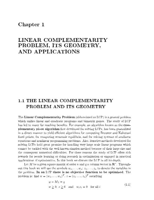
The Linear Complementarity Problem (abbreviated as LCP) is a general problem
which uni es linear and quadratic programs and bimatrix games. The study of LCP
has led to many far reaching bene ts. For example, an algorithm known as the complementary
pivot algorithm rst developed for solving LCPs, has been generalized
in a direct manner to yield e cient algorithms for computing Brouwer and Kakutani
xed points, for computing economic equilibria, and for solving systems of nonlinear
equations and nonlinear programming problems. Also, iterative methods developed for
solving LCPs hold great promise for handling very large scale linear programs which
cannot be tackled with the well known simplex method because of their large size and
the consequent numerical di culties. For these reasons the study of LCP o ers rich
rewards for people learning or doing research in optimization or engaged in practical
applications of optimization. In this book we discuss the LCP in all its depth.
Let M beagiven square matrix of order n and q a column vector in R n . Throughout
this book we will use the symbols w1:::wn z1:::zn to denote the variables in
the problem. In an LCP there is no objective function to be optimized. The
problem is: nd w =(w1:::wn) T , z =(z1:::zn) T satisfying
w ; Mz = q
w > = 0 z > = 0 and wizi =0 for all i
(1:1)

2 Chapter 1. Linear Complementarity Problem, Its Geometry, and Applications
The only data in the problem is the column vector q and the square matrix M. So we
will denote the LCP of nding w 2 R n , z 2 R n satisfying (1.1) by the symbol (q M).
It is said to be an LCP of order n. 8In
an9LCP of8order n there are 2n variables. As
a speci c example, let n =2,M = >: 2 1>,
q = >:
1 2
;5
9
>. This leads to the LCP
;6
w1 ; 2z1; z2 = ;5
w2 ; z1;2z2 = ;6:
w1w2z1z2 > = 0 and w1z1 = w2z2 =0:
The problem (1.2) can be expressed in the form of a vector equation as
w1
8
9
8
9
8
9
(1:2)
>: 1>
+ >: w2
0
0>
+ >: z1
1
;2>
+ >: z2
;1
;1>
= >:
;2
;5>
;6
(1:3)
w1w2z1z2 > = 0 and w1z1 = w2z2 =0 (1:4)
In any solution satisfying (1.4), at least one of the variables in each pair (wjzj),
has to equal zero. One approach for solving this problem is to pick one variable from
each of the pairs (w1z1), (w2z2) and to x them at zero value in (1.3). The remaining
variables in the system may be called usable variables. After eliminating the zero
variables from (1.3), if the remaining system has a solution in which the usable variables
are nonnegative, that would provide a solution to (1.3) and (1.4).
Pick w1, w2 as the zero-valued variables. After setting w1, w2 equal to 0 in (1.3),
the remaining system is
-2 () -1
z1
8
9
8
9
8
8
>: ;2>
+ >: z2
;1
;1>
= >:
;2
;5>
=
;6
-1 ( -2)
q
2
z1 > = 0 z2 > = 0
q1
9
9
8
8
>: q1
9
> = q
q2
9
(1:5)
Figure 1.1 A Complementary Cone
Equation (1.5) has a solution i the vector q can be expressed as a nonnegative
linear combination of the vectors (;2 ;1) T and (;1 ;2) T . The set of all nonnegative

1.1. The Linear Complementarity Problem and its Geometry 3
linear combinations of (;2 ;1) T and (;1 ;2) T is a cone in the q1q2-space as in
Figure 1.1. Only if the given vector q = (;5 ;6) T lies in this cone, does the LCP
(1.2) have a solution in which the usable variables are z1z2. We verify that the point
(;5 ;6) T does lie in the cone, that the solution of (1.5) is (z1z2) = (4=3 7=3) and,
hence, a solution for (1.2) is (w1w2 z1z2) = (0 0 4=3 7=3). The cone in Figure 1.1
is known as a complementary cone associated with the LCP (1.2). Complementary
cones are generalizations of the well-known class of quadrants or orthants.
1.1.1 Notation
The symbol I usually denotes the unit matrix. If we want to emphasize its order, we
denote the unit matrix of order n by the symbol In.
We will use the abbreviation LP for \Linear Program" and BFS for \Basic Feasible
Solution". See [1.28, 2.26]. LCP is the abbreviation for \Linear Complementarity
Problem" and NLP is the abbreviation for \Nonlinear Program".
Column and Row Vectors of a Matrix
If A = (aij) is a matrix of order m n say, we will denote its jth column vector
(a1j:::amj) T by the symbol A.j, and its ith row vector (ai1:::ain) by Ai..
Nonnegative, Semipositive, Positive Vectors
Let x = (x1:::xn) T 2 R n . x >
=
0, that is nonnegative, if xj > =
0 for all j. Clearly,
0 >
=
0. x is said to be semipositive, denoted by x 0, if xj > =
0 for all j and at least
one xj > 0. Notice the distinction in the symbols for denoting nonnegative (>
=
with
two lines under the >) and semipositive ( with only a single line under the >). 0 6 0,
the zero vector is the only nonnegative vector which is not semipositive. Also, if x 0,
Pn j=1 xj > 0. The vector x>0, strictly positive, if xj > 0 for all j. Given two vectors
x y 2 R n we write x >
=
y, if x ; y >
=
0, x y if x ; y 0, and x>yif x ; y>0.
Pos Cones
If fx1:::xrg R n , the cone fx : x = 1x1 + :::+ rxr 1::: r > =
0g is denoted
by Posfx1:::xrg. Given the matrix A of order m n, Pos(A) denotes the cone
PosfA.1:::A.ng = fx : x = A for =( 1::: n) T >
=
0g.
Directions, Rays, Half-Lines, and Step Length
Any point y 2 R n , y 6= 0, de nes a direction in R n . Given the direction y, it's ray
is the half-line obtained by joining the origin 0 to y and continuing inde nitely in the

4 Chapter 1. Linear Complementarity Problem, Its Geometry, and Applications
same direction, it is the set of points f y : > = 0g. Given x 2 R n , by moving from
x in the direction y we get points of the form x + y where > = 0, and the set of all
such points fx + y : > = 0g is the hal ine or ray through x in the direction y. The
point x + y for >0issaidtohave been obtained by moving from x in the direction
y a step length of . As an example, if y =(1 1) T 2 R n , the ray of y is the set of all
points of the form f( ) T : > = 0g. In addition, if, x =(1 ;1) T , the hal ine through
x in the direction y is the set of all points of the form f(1 + ;1+ ) T : > = 0g. See
Figure 1.2. In this half-line, letting =9,we get the point (10 8) T , and this point is
obtained by taking a step of length 9 from x =(1 ;1) T in the direction y =(1 1) T .
1.1.2 Complementary Cones
y
x
y
Ray of
x
Half-line or ray through
in the direction of y
Figure 1.2 Rays and Half-Lines
In the LCP (q M), the complementary cones are de ned by the matrix M. The point
q does not play any role in the de nition of complementary cones.
Let M be a given square matrix of order n. For obtaining C(M), the class of
complementary cones corresponding to M, the pair of column vectors (I.j ;M.j) is

1.1. The Linear Complementarity Problem and its Geometry 5
known as the jth complementary pair of vectors, 1 <
=
j <
=
n. Pick a vector from
the pair (I.j ;M.j) and denote it by A.j. The ordered set of vectors (A.1:::A.n) is
known as a complementary set of vectors. The cone Pos(A.1:::A.n) =fy : y =
1A.1 + :::+ nA.n 1 > = 0::: n > =
0g is known as a complementary cone in the
class C(M). Clearly there are 2n complementary cones.
Example 1.1
Let n =2andM = I. In this case, the class C(I) is just the class of orthants in R 2 . In
general for any n, C(I) is the class of orthants in R n . Thus the class of complementary
cones is a generalization of the class of orthants. See Figure 1.3. Figures 1.4 and 1.5
provide some more examples of complementary cones. In the example in Figure 1.5
since fI.1 ;M.2g is a linearly dependent set, the cone Pos(I.1 ;M.2) has an empty
interior. It consists of all the points on the horizontal axis in Figure 1.6 (the thick
axis). The remaining three complementary cones have nonempty interiors.
Pos( I 2
1
I 1 , )
I
1
Pos( I , I 2 )
I
I
2
2
I
1
Pos( M 1,
I 2 )
I
2
Pos( , )
I 1 I 2
Pos( I 1 , M 2 )
Pos( I 1 , I 2 ) Pos( I 1 , I 2 )
M 2
Pos(
M 1
M 1 , M 2 )
Figure 1.3 When M = I, the Complementarity Cones are the Orthants.
Figure 1.4 Complementary Cones when M = >: 2 ;1>.
1 3
8
9
I
1

6 Chapter 1. Linear Complementarity Problem, Its Geometry, and Applications
Degenerate, Nondegenerate Complementary Cones
Let Pos(A.1:::A.n) be a complementary cone in C(M). This cone is said to be a nondegenerate
complementary cone if it has a nonempty interior, that is if fA.1:::A.ng
is a linearly independent set degenerate complementary cone if its interior is empty,
which happens when fA.1:::A.ng is a linearly dependent set. As examples, all the
complementary cones in Figures 1.3, 1.4, 1.5, are nondegenerate. In Figure 1.6 the
complementary cone Pos(I.1 ;M.2) is degenerate, the remaining three complementary
cones are nondegenerate.
M 2
I
2
I
1
M 1
Figure 1.5 Complementary Cones when M =
Figure 1.6 Complementary Cones when M =
M 2
1.1.3 The Linear Complementary Problem
8
>:
8
>:
M 1
;2 1
1 9;2
1 1>.
2 0
Given the square matrix M of order n and the column vector q 2 R n ,theLCP(q M),
is equivalent to the problem of nding a complementary cone in C(M) that contains
the point q, that is, to nd a complementary set of column vectors (A.1:::A.n) such
that
(i) A.j 2fI.j ;M.jg for 1 < = j < = n
(ii) q can be expressed as a nonnegative linear combination of (A.1:::A.n)
I
9
>.
2
I
1

1.1. The Linear Complementarity Problem and its Geometry 7
where I is the identity matrix of order n and I.j is its jth column vector. This is
equivalent to nding w 2 R n , z 2 R n satisfying P n
j=1 I.jwj ; P n
j=1 M.jzj = q wj > = 0
zj > = 0 for all j, and either wj =0or zj =0for all j. In matrix notation this is
w ; Mz = q (1:6)
w > = 0 z > = 0 (1:7)
wjzj =0 for all j: (1:8)
Because of (1.7), the condition (1.8) is equivalent to Pn j=1 wjzj = wT z =0this condition
is known as the complementarity constraint. In any solution of the LCP
(q M), if one of the variables in the pair (wjzj) is positive, the other should be zero.
Hence, the pair (wjzj) isknown as the jth complementary pair of variables and
each variable in this pair is the complement of the other. In (1.6) the column vector
corresponding to wj is I.j, and the column vector corresponding to zj is ;M.j. For
j = 1 to n, the pair (I.j ;M.j) is the jth complementary pair of column vectors in
the LCP (q M). For j = 1 to n, let yj 2 fwjzjg and let A.j be the column vector
corresponding to yj in (1.6). So A.j 2 fI.j ; M.jg. Then y = (y1:::yn) is a complementary
vector of variables in this LCP, the ordered set (A.1:::A.n) is the
complementary set of column vectors corresponding to it and the matrix A
with its column vectors as A.1:::A.n in that order is known as the complementary
matrix corresponding to it. If fA.1:::A.ng is linearly independent, y is a
complementary basic vector of variables in this LCP, and the complementary
matrix A whose column vectors are A.1:::A.n in that order, is known as the complementary
basis for (1.6) corresponding to the complementary basic vector y. The
cone Pos(A.1:::A.n) = fx : x = 1A.1 + :::+ nA.n 1 > = 0::: n > =
0g is the
complementary cone in the class C(M) corresponding to the complementary set of
column vectors (A.1:::A.n), or the associated complementary vector of variables y.
A solution of the LCP (q M), always means a (w z) satisfying all the constraints
(1.6), (1.7), (1.8).
A complementary feasible basic vector for this LCP is a complementary basic
vector satisfying the property thatqcan be expressed as a nonnegative combination of
column vectors in the corresponding complementary basis. Thus each complementary
feasible basic vector leads to a solution of the LCP.
The union of all the complementary cones associated with the square matrix M
is denoted by the symbol K(M). K(M) is clearly the set of all vectors q for which the
LCP (q M) has at least one solution.
We will say that the vector z leads to a solution of the LCP (q M) i (w =
Mz + q z) is a solution of this LCP.
As an illustration, here are all the complementary vectors of variables and the
corresponding complementary matrices for (1.2), an LCP of order 2.

8 Chapter 1. Linear Complementarity Problem, Its Geometry, and Applications
Complementary The corresponding
vector of variables complementary matrix
(w1w2)
(w1z2)
(z1w2)
(z1z2)
8
>:
8
>:
8
>:
8
>:
1 0
0 1
1 ;1
0 ;2
;2 0
;1 1
;2 ;1
;1 ;2
Since each of these complementary matrices is nonsingular, all the complementary
vectors are complementary basic vectors, and all the complementary matrices are
complementary bases, in this LCP. Since q = (;5 ;6) T in (1.2) can be expressed
as a nonnegative combination of the complementary matrix corresponding to (z1z2)
(z1z2) is a complementary feasible basic vector for this LCP. The reader should draw
all the complementary cones corresponding to this LCP on the two dimensional Cartesian
plane, and verify that for this LCP, their union, the set K(M) =R 2 .
The Total Enumeration Method for the LCP
Consider the LCP (q M) of order n. The complementarity constraint (1.8) implies
that in any solution (w z) of this LCP, foreach j =1to n, we must have
either wj =0
or zj =0:
This gives the LCP a combinatorial, rather than nonlinear avour. It automatically
leads to an enumeration method for the LCP.
There are exactly 2 n complementary vectors of variables. Let
y r =(y r 1:::y r n) r =1 to 2 n
where yr j 2fwjzjg for each j =1ton, be all the complementary vectors of variables.
Let Ar be the complementary matrix corresponding to yr , r = 1 to 2n . Solve the
following system (Pr).
Ary r = q
y r (Pr)
>
=
0 :
This system can be solved by Phase I of the simplex method for LP,orby other methods
for solving linear equality and inequality systems. If this system has a feasible solution,
y r , say, then
y r = y r
all variables not in y r , equal to zero
9
>
9
>
9
>
9
>

1.2. Application to Linear Programming 9
is a solution of LCP (q M). If the complementary matrix Ar is singular, the system
(Pr) may have no feasible solution, or have one or an in nite number of feasible solutions.
Each feasible solution of (Pr) leads to a solution of the LCP (q M) as discussed
above. When this is repeated for r =1to 2 n , all solutions of the LCP (q M) can be
obtained. The method discussed at the beginning of Section 1.1 to solve an LCP of
order 2 is exactly this enumeration method.
This enumeration method is convenient to use only when n = 2, since 2 2 = 4 is
small and to check whether the system (Pr) has a solution for any r, we can draw the
corresponding complementary cone in the two dimensional Cartesian plane and check
whether it contains q. When n>2, particularly for large n, this enumeration method
becomes impractical since 2 n grows very rapidly. In Chapter 2 and later chapters we
discuss e cient pivotal and other methods for solving special classes of LCPs that arise
in several practical applications. In Section 8.7 we show that the general LCP is a hard
problem. At the moment, the only known algorithms which are guaranteed to solve
the general LCP are enumerative methods, see Section 11.3.
1.2 APPLICATION TO
LINEAR PROGRAMMING
In a general LP there may be some inequality constraints, equality constraints, sign
restricted variables and unrestricted variables. Transform each lower bounded variable,
say xj > = lj, into a nonnegative variable by substituting xj = lj + yj where yj > = 0.
Transform each sign restricted variable of the form xj < =
0into a nonnegative variable
by substituting xj = ;yj where yj > =
0. Eliminate the unrestricted variables one
after the other, using the equality constraints (see Chapter 2 of [1.28 or 2.26]). In the
resulting system, if there is still an equality constraint left, eliminate a nonnegative
variable from the system using it, thereby transforming the constraintinto an inequality
constraint in the remaining variables. Repeat this process until there are no more
equality constraints. In the resulting system, transform any inequality constraint of
the \<
=
" form into one of \>
=
" form, bymultiplying both sides of it by `-1'. If the objetive
function is to be maximized, replace it by its negative which should be minimized, and
eliminate any constant terms in it. When all this work is completed, the original LP
is transformed into:
Minimize cx
Subject to Ax >
=
b
(1:9)
x >
=
0
which isinsymmetric form. Here, suppose A is of order m N. If x is an optimum
feasible solution of (1.9), by the results of the duality theory of linear programming
(see [1.28, 2.26]) there exists a dual vector y 2 R m , primal slack vector v 2 R m , and
dual slack vector u 2 R N which together satisfy

10 Chapter 1. Linear Complementarity Problem, Its Geometry, and Applications
8
9
>: u>
;
v
8
>: u
9
> >
v =
0
8
>:
8
9
9
0 ;AT >
A 0
8 >: x>
=
y
>: x
9 8
> >
y =
0 and >: u
v
8
>: cT
9
;b
9
>
9
> T 8 >: x
y
> =0:
(1:10)
Conversely, if u, v, x, y together satisfy all the conditions in (1.10), x is an optimum
solution of (1.9). In (1.10) all the vectors and matrices are written in partitioned
form. For example, ; u
v is the vector (u1:::uNv1:::vm) T . If n = m + N,
w =
8
>: u
v
9
> z =
8
>: x
y
9
> M =
8
>:
0 ;AT
A 0
9
> q =
8
>: cT
9
>
;b
(1.10) is seen to be an LCP of order n of the type (1.6) to (1.8). Solving the LP (1.9)
can be achieved by solving the LCP (1.10).
Also, the various complementary pairs of variables in the LCP (1.10) are exactly
those in the pair of primal, dual LPs (1.9) and its dual. As an example consider the
following LP.
Minimize ;13x1 +42x2
Subject to 8x1 ; x2 + 3x2 > = ;16
; 3x1 + 2x2 ; 13x3 > = 12
xj > =
0 j = 1 2 3:
Let (v1y1), (v2y2) denote the nonnegative slack variable, dual variable respectively,
associated with the two primal constraints in that order. Let u1, u2, u3 denote the
nonnegative dual slack variable associated with the dual constraint corresponding to
the primal variable x1, x2, x3, in that order. Then the primal and dual systems
together with the complementary slackness conditions for optimality are
8x1 ; x2 + 3x3 ; v1 = ;16
;3x1 + 2x2 ; 13x3 ; v2 = 12
8y1 ; 3y2 + u1 = ;13
; y1 + 2y2 + u2 = 42
3y1 ; 13y2 + u3 = 0:
xjujyivi > =
0 for all i j.
xjuj = yivi =0 for all i j.

This is exactly the following LCP.
1.3. Quadratic Programming 11
u1 u2 u3 v1 v2 x1 x2 x3 y1 y2
1 0 0 0 0 0 0 0 8 ;3 ;13
0 1 0 0 0 0 0 0 ;1 2 42
0 0 1 0 0 0 0 0 3 ;13 0
0 0 0 1 0 ;8 1 ;3 0 0 16
0 0 0 0 1 3 ;2 13 0 0 ;12
All variables > = 0. u1x1 = u2x2 = u3x3 = v1y1 = v2y2 =0.
1.3 QUADRATIC PROGRAMMING
Using the methods discussed in Section 1.2 any problem in which a quadratic objective
function has to be optimized subject to linear equality and inequality constraints can
be transformed into a problem of the form
Minimize Q(x) =cx + 1
2 xT Dx
Subject to Ax > = b
x > = 0
(1:11)
where A is a matrix of order m N, and D is a square symmetric matrix of order
N. There is no loss of generality in assuming that D is a symmetric matrix, because if
it is not symmetric replacing D by (D + D T )=2 (which is a symmetric matrix) leaves
Q(x) unchanged. We assume that D is symmetric.
1.3.1 Review on Positive Semide nite Matrices
A square matrix F =(fij) of order n, whether it is symmetric or not, is said to be a
positive semide nite matrix if y T Fy > = 0 for all y 2 R n . It is said to be a positive
de nite matrix if y T Fy > 0 for all y 6= 0. We will use the abbreviations PSD, PD
for \positive semide nite" and \positive de nite", respectively.
Principal Submatrices, Principal Subdeterminants
Let F = (fij) be a square matrix of order n. Let fi1:::irg f1:::ng with its
elements arranged in increasing order. Erase all the entries in F in row i and column
i for each i 62 fi1:::irg. What remains is a square submatrix of F of order r:

12 Chapter 1. Linear Complementarity Problem, Its Geometry, and Applications
8
>:
fi1i1 ::: fi1ir
.
firi1 ::: firir
This submatrix is known as the principal submatrix of F determined by the subset
fi1:::irg. Denoting the subset fi1:::irg by J, we denote this principal submatrix
by the symbol FJJ. It is (fij : i 2 Jj 2 J). The determinant of this principal
submatrix is called the principal subdeterminant ofF determined by the subset J. The
principal submatrix of F determined by , the empty set, is the empty matrix which
has no entries. Its determinant is de ned by convention to be equal to 1. The principal
submatrix of F determined by f1:::ng is F itself. The principal submatrices of F
determined by nonempty subsets of f1:::ng are nonempty principal submatrices
of F . Since the number of distinct nonempty subsets of f1:::ng is 2n ; 1, there are
2n ;1 nonempty principal submatrices of F . The principal submatrices of F determined
by proper subsets of f1:::ng are known as proper principal submatrices of F .
So each proper principal submatrix of F is of order <
=
n ; 1.
Example 1.2
Let
F =
8
>:
..
9
> :
9
0 ;1 2
1 3 4>
1 5 ;3
:
0 2
The principal submatrix corresponding to the subset f1 3g is >. The princi-
1 ;3
pal submatrix corresponding to the subset f2g is 3, the second element in the principal
diagonal of F .
Several results useful in studying P(S)D matrices will now be discussed.
Results on P(S)D Matrices
Result 1.1 If B = (b11) is a matrix of order 1 1, it is PD i b11 > 0, and it is
PSD i b11 > = 0.
Proof. Let y =(y1) 2 R 1 . Then y T By = b11y 2 1 . So y T By > 0 for all y 2 R 1 , y 6= 0,
i b11 > 0, and hence B is PD i b11 > 0. Also y T By > = 0 for all y 2 R 1 , i b11 > = 0,
and hence B is PSD i b11 > = 0.
Result 1.2 If F is a PD matrix all its principal submatrices must also be PD.
Proof. Consider the principal submatrix, G, generated by the subset f1 2g.
G =
8
>: f11 f12
f21 f22
9
> : Let t =
8
>: y1
y2
9
> :
8
>:
9

1.3. Quadratic Programming 13
Pick y =(y1y2 0 0:::0) T . Then y T Fy = t T Gt. However, since F is PD, y T Fy > 0
for all y 6= 0. So t T Gt > 0 for all t 6= 0. Hence, G is PD too. A similar argument can
be used to prove that every principal submatrix of F is also PD.
Result 1.3 If F is PD, fii > 0 for all i. This follows as a corollary of Result 1.2.
Result 1.4 If F is a PSD matrix, all principal submatrices of F are also PSD. This
is proved using arguments similar to those in Result 1.2.
Result 1.5 If F is PSD matrix, fii > =
0 for all i. This follows from Result 1.4.
Result 1.6 Suppose F is a PSD matrix. If fii =0,then fij + fji =0for all j.
Proof. To be speci c let f11 be 0 and suppose that f12 + f21 6= 0. By Result 1.4 the
principal submatrix 8
>: f11
9
f12
f21 f22
> =
8
>:
0 f12
f21 f22
must be PSD. Hence f22y 2 2 +(f12 + f21)y1y2 > = 0 for all y1y2. Since f12 + f21 6= 0,
take y1 = (;f22 ; 1)=(f12 + f21) and y2 = 1. The above inequality is violated since
the left-hand side becomes equal to ;1, leading to a contradiction.
Result 1.7 If D is a symmetric PSD matrix and dii = 0, then D.i = Di. =0. This
follows from Result 1.6.
De nition: The Gaussian Pivot Step
Let A =(aij) be a matrix of order m n. A Gaussian pivot step on A, with row r as
the pivot row and column s as the pivot column can only be carried out if the element
lying in both of them, ars, is nonzero. This element ars is known as the pivot element
for this pivot step. The pivot step subtracts suitable multiples of the pivot row from
each row i for i>rso as to transform the entryinthisrow and the pivot column into
zero. Thus this pivot step transforms
A =
into
8
>:
8
>:
9
>
a11 ::: a1s ::: a1n
.
.
ar1 ::: ars ::: arn
ar+11 ::: ar+1s ::: ar+1n
.
.
.
am1 ::: ams ::: amn
a11 ::: a1s ::: a1n
.
.
ar1 ::: ars ::: arn
a 0 r+11 ::: 0 ::: a 0 r+1n
.
.
.
.
a 0 m1 ::: 0 ::: a 0 mn
.
.
9
>
9
>

14 Chapter 1. Linear Complementarity Problem, Its Geometry, and Applications
where a 0
ij = aij ; (arjais)=ars, fori = r +1tom, j =1ton. As an example consider
the Gaussian pivot step in the following matrix with row 2 as the pivot row and column
3 as the pivot column. The pivot element is inside a box.
8
>:
1 ;2 10 ;4 ;1
4 6 2 ;8 ;4
;3 1 ; 1 2 3
1 ;4 2 3 0
This Gaussian pivot step transforms this matrix into
8
>:
1 ; 2 10 ; 4 ;1
4 6 2 ; 8 ;4
;1 4 0 ; 2 1
;3 ;10 0 11 4
Result 1.8 Let D be a square symmetric matrix of order n > = 2. Suppose D is PD.
Subtract suitable multiples of row 1fromeach of the other rows so that all the entries
in column 1 except the rst is transformed into zero. That is, transform
D =
2
6
4
d11 ::: d1n
d21 ::: d2n
.
.
dn1 ::: dnn
3
7
5 into D1 =
2
6
4
9
>
9
>
d11 ::: d1n
0 d22
~ ::: d2n
~
.
.
.
0 dn2
~ ::: dnn
~
by a Gaussian pivot step with row 1 as pivot row and column 1 as pivot column, clearly
~dij = dij ; d1jdi1=d11 for all i j > = 2. E1, the matrix obtained by striking o the rst
row and the rst column from D1, isalso symmetric and PD.
Also, if D is an arbitrary square symmetric matrix, it is PD i d11 > 0 and the
matrix E1 obtained as above is PD.
Proof. Since D is symmetric dij = dji for all i j. Therefore,
y T Dy =
nX
nX
i=1 j=1
= d11 y1 +
yiyjdij = d11y 2 1 +2y1
nX
j=2
d1jyj =d11
2
nX
j=2
+ X
ij> = 2
d1jyj + X
ij> = 2
yi ~ dijyj :
3
7
5
yiyjdij
Letting y1 = ;( P n
j=2 d1jyj)=d11, weverify that if D is PD, then P ij> = 2 yi ~ dijyj > 0 for
all (y2:::yn) 6= 0,which implies that E1 is PD. The fact that E1 is also symmetric
is clear since ~ dij = dij ; d1jdi1=d11 = ~ dji by the symmetry of D. If D is an arbitrary
symmetric matrix, the above equation clearly implies that D is PD i d11 > 0 and E1
is PD.

1.3. Quadratic Programming 15
Result 1.9 A square matrix F is PD (or PSD) i F + F T is PD (or PSD).
Proof. This follows because x T (F + F T )x =2x T Fx.
8
9
Result 1.10 Let F be a square matrix of order n and E a matrix of order m n.
The square matrix A = >: F ;ET > of order (m + n) is PSD i F is PSD.
E 0
Proof. Let =(y1:::ynt1:::tm) T 2 R n+m and y =(y1:::yn) T . For all , we
have T A = y T Fy. So T A > = 0 for all 2 R n+m i y T Fy > = 0 for all y 2 R n . That
is, A is PSD i F is PSD.
Result 1.11 If B is a square nonsingular matrix of order n, D = B T B is PD and
symmetric.
Proof. The symmetry follows because D T = D. For any y 2 R n , y 6= 0, y T Dy =
y T B T By = kyBk 2 > 0 since yB 6= 0 (because B is nonsingular, y 6= 0 implies yB 6= 0).
So D is PD.
Result 1.12 If A is any matrix of order m n, A T A is PSD and symmetric.
Proof. Similar to the proof of Result 1.11.
Principal Subdeterminants of PD, PSD Matrices
We will need the following theorem from elementary calculus.
Theorem 1.1 Intermediate value theorem: Let f( ) be a continuous real valued
function de ned on the closed interval 0 < = < = 1 where 0 < 1. Let f be a real
number strictly between f( 0) and f( 1). Then there exists a satisfying 0 < < 1,
and f( )=f.
For a proof of Theorem 1.1 see books on calculus, for example, W. Rudin, Principles
of Mathematical Analysis, McGraw-Hill, second edition, 1964, p. 81. Theorem
1.1 states that a continuous real valued function de ned on a closed interval, assumes
all intermediate values between its initial and nal values in this interval.
Now we will resume our discussion of PD, PSD matrices.
Theorem 1.2 If F is a PD matrix, whether it is symmetric or not, the determinant
of F is strictly positive.
Proof. Let F be of order n. Let I be the identity matrix of order n. If the determinant
of F is zero, F is singular, and hence there exists a nonzero column vector x 2 R n such
that x T F = 0, which implies that x T Fx = 0, a contradiction to the hypothesis that F

16 Chapter 1. Linear Complementarity Problem, Its Geometry, and Applications
is PD. So the determinant of F is nonzero. In a similar manner we conclude that the
determinant ofany PD-matrix is nonzero. For 0 < 0 for all 0 < = < = 1 because F is PD. So F ( )
is a PD matrix for all 0 < = < = 1. So from the above argument f( ) 6= 0 for any
satisfying 0 < = < = 1. Clearly, f(0) = 1, and f(1) = determinant of F . If f(1) < 0
by Theorem 1.1 there exists a satisfying 0 < < 1 and f( ) = 0, a contradiction.
Hence f(1) 6< 0. Hence the determinant of F cannot be negative. Also it is nonzero.
Hence the determinant of F is strictly positive.
Theorem 1.3 If F is a PD matrix, whether it is symmetric or not, all principal
subdeterminants of F are strictly positive.
Proof. This follows from Result 1.2 and Theorem 1.2.
Theorem 1.4 If F is a PSD matrix, whether it is symmetric or not, its determinant
is nonnegative.
Proof. For 0 < = < = 1, de ne F ( ), f( ) as in the proof of Theorem 1.2. Since I is
PD, and F is PSD F ( ) is a PD matrix for 0 < = < 1. f(0) = 1, and f(1) is the
determinant of F . If f(1) < 0, there exists a satisfying 0 < :
d11 ::: d1n d1n+1
.
dn1 ::: dnn dnn+1
dn+11 ::: dn+1n dn+1n+1
.
.
9
>
D =
8
>:
d11 ::: d1n
.
.
dn1 ::: dnn
be symmetric matrices. H is of order n +1 and D is a principal submatrix of H.
So dij = dji for all i, j = 1 to n +1. Let x 2 R n , d = (d1n+1:::dnn+1) T , and
Q(x) =x T Dx+2d T x + dn+1n+1. Suppose D is a PD matrix. Let x = ;D ;1 d. Then
x is the point which minimizes Q(x) over x 2 R n , and
Q(x )= (determinant ofH) / (determinant of D). (1:12)
9
>

Also for any x 2 R n
Proof. Since H is symmetric @Q(x)
@x
which satis es @Q(x)
@x
1.3. Quadratic Programming 17
Q(x) =Q(x )+(x ; x ) T D(x ; x ): (1:13)
=0. Also Dx = ;d implies
= 2(Dx + d). Hence x is the only point in Rn
Q(x )=x T
Dx +2d T x + dn+1n+1
= d T x + dn+1n+1 :
(1:14)
For i = 1 to n +1, if gin+1 = din+1 + P n
j=1 dijx j , and if g = (g1n+1:::gnn+1) T ,
then g = d + Dx =0. Also gn+1n+1 = dn+1n+1 + d T x = Q(x ) from (1.14). Now,
from the properties of determinants, it is well known that the value of a determinant
is unaltered if a constant multiple of one of its columns is added to another. For j =1
to n, multiply the jth column of H by x j and add the result to column n +1of H.
This leads to
Determinant of H = determinant of
= determinant of
8
>:
8
>:
= (Q(x )) (determinant of D)
d11 ::: d1n g1n+1
.
.
.
dn1 ::: dnn gnn+1
dn+11 ::: dn+1n gn+1n+1
d11
.
::: d1n
.
0
.
dn1 ::: dnn 0
dn+11 ::: dn+1n Q(x )
which yields (1.12). (1.13) can be veri ed by straight forward expansion of its right
hand side, or it also follows from Taylor expansion of Q(x) around x , since @2Q(x) @x2 =
2D and x satis es @Q(x)
@x =0.Since D is a PD matrix, wehave(x;x )T D(x;x ) > 0,
for all x 2 R n , x 6= x . This and (1.13) together imply that: Q(x) > Q(x ), for all
x 2 R n , x 6= x . Hence x is the point which minimizes Q(x) over x 2 R n .
Theorem 1.7 Let H, D be square, symmetric matrices de ned as in Theorem 1.6.
H is PD i D is PD and the determinant of H is strictly positive.
Proof. Suppose H is PD. By Theorem 1.2 the determinant of H is strictly positive,
and by Result 1.2 its principal submatrix D is also PD.
Suppose that D is PD and the determinant ofH is strictly positive. Let x =(x1
:::xn) T and =(x1:::xnxn+1) T . De ne d, Q(x) as in Theorem 1.6. If xn+1 =0,
but 6= 0 (i. e., x 6= 0), T H = x T Dx > 0, since D is PD. Now suppose xn+1 6= 0.
Let = (1=xn+1)x. Then T H = x T Dx +2xn+1d T x + dn+1n+1x 2 n+1 = x 2 n+1Q( ).
9
>
9
>

18 Chapter 1. Linear Complementarity Problem, Its Geometry, and Applications
So, when xn+1 6= 0, T H = x 2 n+1Q( ) > = x 2 n+1 (minimum value of Q( ) over 2 R n )
= x 2 n+1 ((determinant ofH)/determinant ofD)) > 0. So under our hypothesis that D
is PD and the determinantofH is strictly positive, wehave T H > 0 for all 2 R n+1 ,
6= 0,that is H is PD.
Theorem 1.8 Let H be the square symmetric matrix de ned in Theorem 1.6. H
is PD i the determinants of these n +1principal submatrices of H,
(d11)
are strictly positive.
8
>: d11
9
d12 >
d21 d22
8
>:
d11 d12 d13
d21 d22 d23
d31 d32 d33
9
> :::DH
Proof. Proof is by induction on the order of the matrix. Clearly, the statement of the
theorem is true if H is of order 1. Now suppose the statement of the theorem is true
for all square symmetric matrices of order n. By this and the hypothesis, we know that
the matrix D is PD. So D is PD and the determinant of H is strictly positive by the
hypothesis. By Theorem 1.7 these facts imply that H is PD too. Hence, by induction,
the statement ofthe theorem is true in general.
Theorem 1.9 A square symmetric matrix is PD i all its principal subdeterminants
are strictly positive.
Proof. Let the matrix be H de ned as in Theorem 1.6. If H is PD, all its principal
subdeterminants are strictly positive by Theorem 1.3. On the other hand, if all the
principal subdeterminants of H are strictly positive, the n+1 principal subdeterminants
of H discussed in Theorem 1.8 are strictly positive, and by Theorem 1.8 this implies
that H is PD.
De nition: P -matrix
A square matrix, whether symmetric or not, is said to be a P -matrix i all its principal
subdeterminants are strictly positive.
8 9 8 9
As examples, the matrices I, >: 2 24>,
>: 2 1>
are P -matrices. The matrices
8 9 8 9 8 9 0 2 2 2
>: 0 1>,
>: ;1 0>,
>: 2 2>
are not P -matrices.
0 1 0 10 2 2
Theorem 1.10 A symmetric P -matrix is always PD.IfaP -matrix is not symmetric,
it may notbe PD.
Proof. By Theorem 1.9 B, a symmetric matrix is PD i it is a P -matrix. Consider
the matrix B, 8
B = >: 1
6
9
0>
1
B + B T 8
= >: 2
6
9
6>
:
2

1.3. Quadratic Programming 19
Since all its principal subdeterminants are 1, B is a P -matrix. However, the determinant
of (B + B T ) is strictly negative, and hence it is not a PD matrix by Theorem
1.9, and by Result 1.9 this implies that B is not PD. Actually, itcan be veri ed that,
(1 ;1)B(1 ;1) T = ;4 < 0.
Note 1.1 The interesting thing to note is that if H is a symmetric matrix, and if
the n+1 principal subdeterminants of H discussed in Theorem 1.8 are strictly positive,
by Theorems 1.10 and 1.8 all principal subdeterminants of H are positive. This result
may not be true if H is not symmetric.
Exercises
1.1 If H is a square symmetric PSD matrix, and its determinant is strictly positive,
then prove that H is a PD matrix. Construct a numerical example to show that this
result is not necessarily true if H is not symmetric.
1.2 Is the following statement true? \H is PSD i its (n+1) principal subdeterminants
discussed in Theorem 1.8 are all nonnegative." Why? Illustrate with a numerical
example.
By Theorem 1.9 the class of PD matrices is a subset of the class of P -matrices.
By Theorem 1.10 when restricted to symmetric matrices, the property of being a PD
matrix is the same as the property of being a P -matrix. An asymmetric P -matrix may
not be PD, it may be a PSD matrix as the matrix f M(n) below is, or it may not even
be a PSD matrix. Let
fM(n) =
8
>:
1 0 0 ::: 0 0
2 1 0 ::: 0 0
2
.
2
.
1
.
:::
. ..
0
.
0
.
2 2 2 ::: 1 0
2 2 2 ::: 2 1
9
>
: (1:15)
fM(n) isalower triangular matrix in which all the diagonal entries are 1, and all entries
below the diagonal are 2. All the principal subdeterminants of fM(n) are clearly equal
to 1, and hence fM(n) isaP -matrix. However, fM(n)+(fM(n)) T is the matrix in which
all the entries are 2, and it can be veri ed that it is a PSD matrix and not a PD matrix.
Theorem 1.11 Let F be a square PSD matrix of order n, whether it is symmetric
or not. If x 2 R n is such that x T F x =0, then (F + F T )x =0.

20 Chapter 1. Linear Complementarity Problem, Its Geometry, and Applications
Proof. Let D = F +F T . D is symmetric and by Result 1.9, D is PSD. For all x 2 R n ,
x T Dx =2x T Fx. So x T Dx =0too. We wish to prove that Dx =0. Let x 2 R n . For
all real numbers (x + x) T D(x + x) > = 0, that is
2 x T Dx +2 x T Dx > = 0 (1:16)
since x T Dx = 0. If x T Dx = 0, by taking = 1 and then ;1 in (1.16), we conclude
that x T Dx = 0. If x T Dx 6= 0, since D is PSD, x T Dx > 0. In this case, from (1.16)
we conclude that 2x T Dx > = ; x T Dx for > 0, and 2x T Dx < = ; x T Dx for < 0.
Taking to be a real number of very small absolute value, from these we conclude
that x T Dx must be equal to zero in this case. Thus whether x T Dx =0,orx T Dx > 0,
we have x T Dx = 0. Since this holds for all x 2 R n , we must have x T D = 0, that is
Dx =0.
Algorithm for Testing Positive De niteness
Let F = (fij) be a given square matrix of order n. Find D = F + F T . F is PD i
D is. To test whether F is PD, we can compute the n principal subdeterminants of
D determined by the subsets f1g f1 2g:::f1 2:::ng. F is PD i each of these n
determinants are positive, by Theorem 1.8. However, this is not an e cient method
unless n is very small, since the computation of these separate determinants is time
consuming.
We now describe a method for testing positive de niteness of F which requires at
most n Gaussian pivot steps on D along its main diagonal hence the computational
e ort required by this method is O(n 3 ). This method is based on Result 1.8.
(i) If any of the principal diagonal elements in D are nonpositive, D is not PD.
Terminate.
(ii) Subtract suitable multiples of row 1 from all the other rows, so that all the entries
in column 1 and rows 2 to n of D are transformed into zero. That is, transform
D into D1 as in Result 1.8. If any diagonal element in the transformed matrix,
D1, is nonpositive, D is not PD. Terminate.
(iii) In general, after r steps we will have a matrix Dr of the form:
2
6
4
d11 d12 ::: d1n
0 d22
~ ::: d1n
~
.
0 ..
.
drr ::: drn
.
.
.
0
.
.
dr+1r+1
^
.
.
::: dr+1n
^
.
.
0 0 0 dnr+1
^ ::: dnn
^
Subtract suitable multiples of row r +1in Dr from rows i for i >r+1,so that
all the entries in column r +1and rows i for i > r +1 are transformed into 0.
3
7
5
:

1.3. Quadratic Programming 21
This transforms Dr into Dr+1. If any element in the principle diagonal of Dr+1
is nonpositive, D is not PD. Terminate. Otherwise continue the algorithm in the
same manner for n ; 1 steps, until Dn;1 is obtained, which is of the form
2
6
4
3
d11
0
.
d12
d22
~
0
.
:::
:::
d1n
d2n
~ 7
. 5
0 0 ::: dnn
:
Dn;1 is upper triangular. That's why this algorithm is called the superdiagonalization
algorithm. If no termination has occured earlier and all the diagonal
elements of Dn;1 are positive, D, and hence, F is PD.
Example 1.3
Test whether
F =
2
6
4
3 1 2 2
;1 2 0 2
0 4 4 5
3
0 ;2 ; 13
3
6
3
7
5 is PD, D = F + F T =
2
6
4
6 0 2 2
0 4 4 0
2 4 8 ; 8
3
2 0 ; 8
3
All the entries in the principal diagonal of D (i. e., the entries dii for all i) are strictly
positive. So apply the rst step in superdiagonalization getting D1. Since all elements
in the principal diagonal of D1 are strictly positive, continue. The matrices obtained
in the order are:
D1 =
D3 =
2
6
4
2
6
4
6 0 2 2
0 4 4 0
0 4 22
3
0 0 ; 10
3
10 ; 3
34
3
6 0 2 2
0 4 4 0
0 0 10
3
10 ; 3
0 0 0 8
3
7
5 D2 =
3
7
5 :
2
6
4
6 0 2 2
0 4 4 0
0 0 10
3
0 0 ; 10
3
10 ; 3
34
3
The algorithm terminates now. Since all diagonal entries in D3 are strictly positive,
conclude that D and, hence, F is PD.
Example 1.4
Test whether D =
8
>:
1 0 2 0
0 2 4 0
2 4 4 5
0 0 5 3
9
>
is PD.
3
7
5
12
3
7
5 :

22 Chapter 1. Linear Complementarity Problem, Its Geometry, and Applications
D is already symmetric, and all its diagonal elements are positive. The rst step of
the algorithm requires performing the operation: (row 3){2(row 1) on D. This leads
to
8 1
0
D1 =
>: 0
0
0
2
4
0
2
4
0
5
9 0
0
5>
3
:
Since the third diagonal element in D1 is not strictly positive, D is not PD.
Algorithm for Testing Positive Semide niteness
Let F = (fij) be the given square matrix. Obtain D = F + F T . If any diagonal
element of D is 0, all the entries in the row and column of the zero diagonal entry
must be zero. Otherwise D (and hence F ) is not PSD and we terminate. Also, if any
diagonal entries in D are negative, D cannot be PSD and we terminate. If termination
has not occurred, reduce the matrix D by striking o the rows and columns of zero
diagonal entries.
Start o by performing the row operations as in (ii) above, that is, transform D
into D1. If any diagonal element in D1 is negative, D is not PSD. Let E1 be the
submatrix of D1 obtained by striking o the rst row and column of D1. Also, if a
diagonal element in E1 is zero, all entries in its row and column in E1 must be zero.
Otherwise D is not PSD. Terminate. Continue if termination does not occur.
In general, after r steps we willhave a matrix Dr as in (iii) above. Let Er be the
square submatrix of Dr obtained by striking o the rst r rows and columns of Dr.
If any diagonal element in Er is negative, D cannot be PSD. If any diagonal element
of Er is zero, all the entries in its row and column in Er must be zero otherwise D is
not PSD. Terminate. If termination does not occur, continue.
Let dss be the rst nonzero (and, hence, positive) diagonal elementinEr. Subtract
suitable multiples of row s in Dr from rows i, i>s, so that all the entries in column
s and rows i, i > s in Dr, are transformed into 0. This transforms Dr into Ds and
we repeat the same operations with Ds. If termination does not occur until Dn;1 is
obtained and, if the diagonal entries in Dn;1 are nonnegative, D and hence F are
PSD.
In the process of obtaining Dn;1, if all the diagonal elements in all the matrices
obtained during the algorithm are strictly positive, D and hence F is not only PSD
but actually PD.
Example 1.5
Is the matrix
2 0
6 2
6 F = 6 3
4 4
;2
3
3
0
;3
3
3
0
;4
0
0
8
3 5
0 7 07
5 4
;5 0 0 4 2
PSD? D = F + F T =
2
6
4
3
0
0
0
0
0
6
6
0
0
6
6
0
0
0
0
16
0
0 7 07
5 8
0 0 0 8 4
:

1.3. Quadratic Programming 23
D.1 and D1. are both zero vectors. So we eliminate them, but we will call the remaining
matrix by the same name D. All the diagonal entries in D are nonnegative. Thus we
apply the rst step in superdiagonalization. This leads to
D1 =
8
>:
6 6 0 0
0 0 0 0
0 0 16 8
0 0 8 4
9
>
E1 =
8
>:
9
0 0 0
0 16 8>
0 8 4
:
The rst diagonal entry in E1 is 0, but the rst column and row of E1 are both zero
vectors. Also all the remaining diagonal entries in D1 are strictly positive. So continue
with superdiagonalization. Since the second diagonal element in D1 is zero, move to
the third diagonal element of D1. This step leads to
D3 =
8
>:
9
6 6 0 0
0 0 0 0
0 0 16 8>
0 0 0 0
:
All the diagonal entries in D3 are nonnegative. D and hence F is PSD but not PD.
Example 1.6
Is the matrix D in Example 1.4 PSD? Referring to Example 1.4 after the rst step in
superdiagonalization, we have
E1 =
8
>:
9
2 4 0
4 0 5>
0 5 3
:
The second diagonal entry in E1 is 0, but the second row and column of E1 are not
zero vectors. So D is not PSD.
1.3.2 Relationship of Positive Semide niteness
to the Convexity of Quadratic Functions
Let ; be a convex subset of R n , and let g(x) be a real valued function de ned on ;.
g(x) issaid to be a convex function on ;, if
g( x 1 +(1; )x 2 ) < = g(x 1 )+(1; )g(x 2 ) (1:17)

24 Chapter 1. Linear Complementarity Problem, Its Geometry, and Applications
for every pair of points x1 , x2 in ;, and for all 0 < <
= =
1. g(x) issaidtobeastrictly
convex function on ; if (1.17) holds as a strict inequality for every pair of distinct
points x1 , x2 in ; (i. e., x1 6= x2 ) and for all 0 < = 0 for all x 1 x 2 2 R n
and 0 < = < = 1, i T D > = 0 for all 2 R n , that is i D (or equivalently F ) is PSD.
Hence f(x) isconvex on R n i F (or equivalently D) is PSD.
Also by the above argument we see that f(x 1 )+(1; )f(x 2 );f( x 1 +(1; )x 2 )
> 0 for all x 1 6= x 2 in R n and 0 < < 1, i T D > 0 for all 2 R n , 6= 0.
Hence f(x) is strictly convex on R n i T D > 0 for all 6= 0, that is i D (or
equivalently F ) is PD. These are the conditions for the convexity or strict convexity
of the quadratic function f(x) over the whole space R n . It is possible for f(x) to
be convex on a lower dimensional convex subset of R n (for example, a subspace of
8
9
R n ) even though the matrix F is not PSD. For example, the quadratic form f(x) =
(x1x2) >: ;1 0>
(x1x2)
0 1
T is convex over the subspace f(x1x2) : x1 = 0g but not
over the whole of R 2 .
Exercise
1.3 Let K R n be a convex set and Q(x) =cx + 1
2 xT Dx. If Q(x) is convex over K
and K has a nonempty interior, prove that Q(x) isconvex over the whole space R n .
1.3.3 Necessary Optimality Conditions
for Quadratic Programming
We will now resume our discussion of the quadratic program (1.11).
Theorem 1.12 If x is an optimum solution of (1.11), x is also an optimum solution
of the LP
minimize (c + xT D)x
subject to Ax >
=
b
x >
=
0 :
(1:18)

1.3. Quadratic Programming 25
Proof. Notice that the vector of decision variables in (1.18) is x x is a given point
and the cost coe cients in the LP (1.18) depend on x. The constraints in both (1.11)
and (1.18) are the same. The set of feasible solutions is a convex polyhedron. Let ^x be
any feasible solution. By convexity of the set of feasible solutions x = ^x+(1; )x =
x + (^x ; x) is also a feasible solution for any 0 < < 1. Since x is an optimum
feasible solution of (1.11), Q(x ) ; Q(x) > = 0, that is (c + x T D)(^x ; x) +(1=2)
2 (^x ; x) T D(^x ; x) > = 0 for all 0 < = (; =2)(^x ; x) T D(^x ; x) for all 0 < = 0, that is, (c + x T D)^x > = (c + x T D)x. Since this must hold for an arbitrary
feasible solution ^x, x must be an optimum feasible solution of (1.18).
Corollary 1.1 If x is an optimum feasible solution of (1.11), there exist vectors
y 2 R m and slack vectors u 2 R N , v 2 R m such that x, y, u, v together satisfy
8
9
>: u>
;
v
8
>: u
9
> >
v =
0
8
>: D ;AT
9
9
8
>
A 0
8 >: x>
=
y
8
>: x
9 8
> >
y =
0 and >: u
v
>: cT
9
;b
9
>
> T 8 >: x
y
9
> =0:
(1:19)
Proof. >From the above theorem x must be an optimum solution of the LP (1.18).
The corollary follows by using the results of Section 1.2 on this fact.
Necessary and Su cient Optimality Conditions
for Convex Quadratic Programs
The quadratic minimization problem (1.11) is said to be a convex quadratic program
if Q(x) is convex, that is, if D is a PSD matrix (by the results in Section
1.3.2, or Theorem 17 of Appendix 3). If D is not PSD, (1.11) is said to be a nonconvex
quadratic program. Associate a Lagrange multiplier yi to the ith constraint
\Ai.x > = bi" i =1to m and a Lagrange multiplier uj to the sign restriction on xj in
(1.11), j =1to N. Let y =(y1:::ym) T , u =(u1:::uN) T . Then the Lagrangian
corresponding to the quadratic program (1.11) is L(x y u)=Q(x);y T (Ax;b);u T x.
The Karush-Kuhn-Tucker necessary optimality conditions for (1.11) are
@L
@x (x y u)=cT + Dx ; A T y ; u =0
y > = 0 u > = 0
y T (Ax ; b) =0 u T x =0
Ax ; b > = 0 x > = 0 :
(1:20)
Denoting the slack variables Ax ; b by v, the conditions (1.20) can be veri ed to
be exactly those in (1.19), written out in the form of an LCP. A feasible solution x

26 Chapter 1. Linear Complementarity Problem, Its Geometry, and Applications
for (1.11), is said to be a Karush-Kuhn-Tucker point (or abbreviated as a KKT
point) if there exist Lagrange multiplier vectors y, u, such that x, y, u together satisfy
(1.20) or the equivalent (1.19). So the LCP (1.19) is the problem of nding a KKT
point for (1.11). We now have the following results.
Theorem 1.13 If x is an optimum solution for (1.11), x mustbeaKKT point for
it, whether Q(x) is convex or not.
Proof. Follows from Theorem 1.12 and Corollary 1.1.
Thus (1.20) or equivalently (1.19) provide the necessary optimality conditions for a
feasible solution x of (1.11) to be optimal. Or, in other words, every optimum solution
for (1.11) must be a KKT point for it. However, given a KKT point for (1.11) we
cannot guarantee that it is optimal to (1.11) in general. In the special case when D
is PSD, every KKT point for (1.11) is optimal to (1.11), this is proved in Theorem
1.14 below. Thus for convex quadratic programs, (1.20) or equivalently (1.19) provide
necessary and su cient optimality conditions.
Theorem 1.14 If D is PSD and x is a KKT point of (1.11), x is an optimum
feasible solution of (1.11).
Proof. >From the de nition of a KKT point and the results in Section 1.2, if x is a
KKT point for (1.11), it must be an optimum feasible solution of the LP (1.18). Let x
be any feasible solution of (1.11).
Q(x) ; Q(x) =(c + x T D)(x ; x)+ 1
2 (x ; x)T D(x ; x) :
The rst term on the right-hand side expression is nonnegative since x is an optimal
feasible solution of (1.18). The second term in that expression is also nonnegative since
D is PSD. Hence, Q(x) ; Q(x) > = 0forall feasible solutions, x, of (1.11). This implies
that x is an optimum feasible solution of (1.11).
Clearly (1.19) is an LCP. An optimum solution of (1.11) must be a KKT point for
it. Solving (1.19) provides a KKT point for (1.11) and if D is PSD, this KKT point is
an optimum solution of (1.11). [If D is not PSD and if a KKT point is obtained when
(1.19) is solved, it may not be an optimum solution of (1.11).]
Example 1.7 Minimum Distance Problem.
Let K denote the shaded convex polyhedral region in Figure 1.7. Let P0 be the point
(;2 ;1). Find the point in K that is closest to P0 (in terms of the usual Euclidean
distance). Such problems appear very often in operations research applications.

1.3. Quadratic Programming 27
01
01
01
01
01
01
01
01
01
00000000000
11111111111
(1,3)
01
00000000000
11111111111
01
P 00000000000
11111111111
1
01
00000000000
11111111111
0
00000000000
11111111111
K
1
01
00000000000
11111111111
01
00000000000
11111111111
01
00000000000
11111111111
01
00000000000
11111111111
01
00000000000
11111111111
01
00000000000
11111111111
P0 01
P2 (4,0)
(-2,-1) 01
01
01
Figure 1.7
Every point inK can be expressed as a convex combination of its extreme points (or
corner points) P1, P2, P3, P4. That is, the coordinates of a general point in K are:
( 1 +4 2 +5 3 +5 4 3 1 +0 2 +2 3 +4 4) where the i satisfy 1 + 2 + 3 + 4 =1
and i > = 0 for all i. Hence, the problem of nding the point in K closest to P0 is
equivalent to solving:
Minimize ( 1 +4 2 +5 3 +5 4 ; (;2)) 2 +(3 1 +2 3 +4 4 ; (;1)) 2
Subject to 1 + 2 + 3 + 4 =1
P 4
P 3
(5,4)
(5,2)
i > =
0 for all i:
4 can be eliminated from this problem by substituting the expression 4 =1; 1; 2;
3 for it. Doing this and simplifying, leads to the quadratic program
Minimize (;66 ;54 ;20) + 1
2
Subject to ; 1 ; 2 ; 3 > = ;1
>
= 0
T
8
>:
34 16 4
16 34 16
4 16 8
where = ( 1 2 3) T . Solving this quadratic program is equivalent to solving the
LCP 8>:
9 u1
u2
u3 > ;
8
98
9
34 16 4 1 1
16 34 16 1 2
>: 4 16 8 1>
>: 3 >
; 1 ; 1 ; 1 0
=
8 9 ;66
;54
>: ;20>
1
:
v1
y1
9
>

28 Chapter 1. Linear Complementarity Problem, Its Geometry, and Applications
All variables u1u2u3v1 1 2 3y1 > = 0
and u1 1 = u2 2 = u3 3 = v1y1 =0:
Let (~u1 ~u2 ~u3 ~v1 ~ 1 ~ 2 ~ 3 ~y1) be a solution to this LCP. Let ~ 4 =1; ~ 1 ; ~ 2 ; ~ 3.
Then ~x =( ~ 1 +4 ~ 2 +5 ~ 3 +5 ~ 4 3 ~ 1 +2 ~ 3 +4 ~ 4) is the point in K that is closest to
P0.
1.3.4 Convex Quadratic Programs and LCPs
Associated with PSD Matrices
Consider the LCP (q M), which is (1.6) { (1.8), in which the matrix M is PSD.
Consider also the quadratic program
Minimize z T (Mz + q)
Subject to Mz + q > = 0
z > = 0 :
This is a convex quadratic programming problem since M is PSD. If the optimum
objectivevalue in this quadratic program is > 0, clearly the LCP (q M) has no solution.
If the optimum objective value in this quadratic program is zero, and z is any optimum
solution for it, then (w = Mz + q z) is a solution of the LCP. Conversely if (~w ~z) is
any solution of the LCP (q M), the optimum objective value in the above quadratic
program must be zero, and ~z is an optimum solution for it. Thus every LCP associated
with a PSD matrix can be posed as a convex quadratic program.
Now, consider a convex quadratic program in which Q(x) =cx+ 1
2 xT Dx (where D
is a symmetric PSD matrix) has to be minimized subject to linear constraints. Replace
each equality constraint by a pair of opposing inequality constraints (for example,
Ax = b is replaced by Ax < = b and Ax > = b). Now the problem is one of minimizing
Q(x) subject to a system of linear inequality constraints. This can be transformed into
an LCP as discussed in Section 1.3.3. The matrix M in the corresponding LCP will
be PSD by Result 1.10, since D is PSD. Thus every convex quadratic programming
problem can be posed as an LCP associated with a PSD matrix.

1.3. Quadratic Programming 29
1.3.5 Applications of Quadratic Programming
The Portfolio Problem
A big investment rm has a total of $ a to invest. It has a list of n stocks in which this
money can be invested. The problem is to determine how much of the available money
should be invested in each stock. The solution of this problem is called a portfolio. In
this problem, it is well known that \one should never put all of their eggs in one basket".
So after a thorough study, the manager of the company has determined a lower bound
$ lj and an upper bound $ kj for the amount to be invested in stock j, j = 1 to n.
The yield from each stock varies randomly from year to year. By the analysis of past
data, j, the expected (or average) yield per dollar invested in stock j per year has
been estimated. The yields from various stocks are not mutually independent, and the
analysis of past data has also provided an estimate of the variance-covariance matrix,
D, forthe annual yields from the various stocks per dollar invested. D is a symmetric
positive de nite matrix of order n. If $ xj is the amount invested in stock j, j =1ton,
the portfolio is x =(x1:::xn) T ,theexpected annual yield from it is Pn j=1 jxj and
the variance of the yield is xT Dx. The variance is a measure of the random uctuation
in the annual yield and hence it should be minimized. The company would, of course,
like to see its expected yield maximized. One way ofachieving both of these objectives
is to specify a target or lower bound, say , on the expected yield and to minimize the
variance subject to this constraint. This leads to the problem:
Minimize xT Dx
Subject to Pn j=1 jxj > P =
xj < = a
which is a quadratic programming problem.
Constrained Linear Regression
lj < = xj < = kj j =1to n
We will illustrate this application with an example of eggs and chickens due to C. Marmolinero
[1.22]. The rst step in chicken farming is hatching, carried out by specialized
hatcheries. When hatched, a day-old-chicken is born. It needs no food for the rst
two days, at the end of which it is called a growing pullet and moved out of the
hatchery. Pullets have to grow over a period of approximately 19 weeks before they
start producing eggs, and this is done by specialized growing units under optimum
conditions of diet, heating, lighting etc. After 19 weeks of age, pullets are moved into
the laying ock and are then called hens. Consider a geographical region, say a State.
Data on the numberofchickens hatched by hatcheries in the state during each month
is available from published state government statistics. But, day-old-chickens may be

30 Chapter 1. Linear Complementarity Problem, Its Geometry, and Applications
bought from, or sold to rms outside the state, statistics on which are not available.
De ne
yt =number (in millions) of growing pullets in the state, on the rst day of
month t.
dt =number (in millions) of day-old-chickens hatched by hatcheries in the
state in month t (from government statistics).
Here dt are not variables, but are the given data. People in the business of producing
chicken feed are very much interested in getting estimates of yt from dt. This provides
useful information to them in their production planning, etc. Not all the day-oldchickens
placed by hatcheries in a month may be alive in a future month. Also, after
ve months of age, they are recorded as hens and do not form part of the population of
growing pullets. So the appropriate linear regression model for yt as a function of the
dt's seems to be yt = 0 + P5 i=1 idt;i, where 0 is the number of pullets in census,
which are not registered as being hatched (pullets imported into the State, or chickens
exported from the State), and i is a survival rate (the proportion of chickens placed in
month t;i that are alive in month t, i = 1 to 5). We, of course, expect the parameters
i to satisfy the constraints
0 < = 5 < = 4 < = 3 < = 2 < = 1 < =
1 : (1:21)
To get the best estimates for the parameters = ( 0 1 2 3 4 5) T from past
data, the least squares method could be used. Given data on yt, dt over a period of
time (say for the last 10 years), de ne L2( )= P t (yt ; 0 ; P5 i=1 idt;i) 2 . Under the
least squares method the best values for are taken to be those that minimize L2( )
subject to the constraints (1.21). This is clearly a quadratic programming problem.
One may be tempted to simplify this problem by ignoring the constraints (1.21)
on the parameters . The unconstrained minimum of L2( ) can be found very easily
by solving the system of equations @L2( )
=0.
@
There are two main di culties with this approach. The rst is that the solution of
this system of equations requires the handling of a square matrix (aij) with aij =1=(i+
j ; 1), known as the Hilbert matrix, which is di cult to use in actual computation
because of ill-conditioning. It magni es the uncertainty in the data by very large
factors. We will illustrate this using the Hilbert matrix of order 2. This matrix is
8
H2 = >: 1 1
3
Consider the following system of linear equations with H2 as the coe cient matrix.
x1
1
1
2
1
2
x2
1
2
1
3
1
3
9
> :
b1
b2

1.3. Quadratic Programming 31
It can be veri ed that the solution of this system of linear equations is x =(4b1 ; 6b2
;6b1 + 12b2) T . Suppose we have the exact value for b1 but only an approximate
value for b2. In the solution x, errors in b2 are magni ed by 12 times in x2, and 6
times in x1. This is only in a small system involving the Hilbert matrix of order 2.
The error magni cation grows very rapidly in systems of linear equations involving
Hilbert matrices of higher orders. In real world applications, the coe cients in the
system of linear equations (constants corresponding to b1, b2 in the above system)
are constructed using observed data, which are always likely to have small errors.
These errors are magni ed in the solution obtained by solving the system of equations,
making that solution very unreliable. See reference [1.36]. The second di culty is
that even if we are able to obtain a reasonable accurate solution ^ for the system of
equations @L2( )
=0, @
^ may violate the constraints (1.21) that the parameter vector
is required to satisfy. For example, when this approach was applied on our problem
with actual data over a 10-year horizon from a State, it led to the estimated parameter
vector ^ =(4:22 1:24:70 ; :13:80) T . We have ^ 4 < 0 and ^ 2 > 1, these values are
not admissible for survival rates. So = ^ does not make any sense in the problem.
For the same problem, when L2( ) was minimized subject to the constraints (1.21),
using a quadratic programming algorithm it gave an estimate for the parameter vector
which was quite good.
Parameter estimation in linear regression using the least squares method is a very
common problem in many statistical applications, and in almost all branches of scienti
c research. In a large proportion of these applications, the parameter values are
known to satisfy one or more constraints (which are usually linear). The parameter estimation
problem in constrained linear regression is a quadratic programming problem
when the constraints on the parameters are linear.
1.3.6 Application of Quadratic Programming
in Algorithms for NLP, Recursive Quadratic
Programming Methods for NLP
Recently, algorithms for solving general nonlinear programs, through the solution
of a series of quadratic subproblems have been developed [1.41 to 1.54]. These methods
are called recursive quadratic programming methods, orsequential quadratic
programming methods, orsuccessive quadratic programming methods in the
literature. Computational tests have shown that these methods are especially e cient
in terms of the number of function and gradient evaluations required. Implementation
of these methods requires e cient algorithms for quadratic programming. We provide
here a brief description of this approach for nonlinear programming. Consider the
nonlinear program:

32 Chapter 1. Linear Complementarity Problem, Its Geometry, and Applications
Minimize (x)
Subject to gi(x) =0 i =1to k
gi(x) > = 0 i = k +1to m
(1:22)
where (x) andgi(x) are real valued twice continuously di erentiable functions de ned
over R n . Let g(x) = (g1(x):::gm(x)) T . Given the Lagrange multiplier vector =
( 1::: k k+1::: m), the Lagrangian corresponding to (1.22) is L(x )= (x) ;
g(x). The rst order (or Karush-Kuhn-Tucker) necessary optimality conditions for
this problem are
rxL(x )=r (x); rg(x) =0
i > =
0
igi(x) =0
i = k +1to m
i = k +1to m
(1:23)
gi(x) =0 i =1to k
gi(x) >
=
0 i = k +1to m:
The methods described here for tackling (1.22) try to obtain a solution x and a Lagrange
multiplier vector ,whichtogether satisfy (1.23), through an iterative process.
In each iteration, a quadratic programming problem is solved, the solution of which
provides revised estimates of the Lagrange multipliers and also determines a search
direction for a merit function. The merit function is an absolute value penalty function
(L1-penalty function) that balances the two competing goals of decreasing (x)
and reducing the amounts by which the constraints are violated. The merit function
is then minimized in the descent direction by using a line minimization procedure.
The solution of this line minimization problem produces a revised point x. With the
revised x and , the method goes to the next iteration. The rst iteration begins with
an initial point x and Lagrange multiplier vector satisfying i > =
0, i = k +1to m.
At the beginning of an iteration, let ^x, ^ be the current vectors. De ne
Q(d) =L(^x ^)+ ; rxL(^x ^) d + 1
2 dT @2L(^x ^)
@x2 d (1:24)
where d = x; ^x. Q(d)istheTaylor series approximation for L(x ^) around the current
point ^x up to the second order. Clearly @2L(^x^) @x2 changes in each iteration. Since this
is an n n matrix, recomputing it in each iteration can be very expensive computationally.
So in computer implementations of this method, @2L(^x^) @x2 is approximated by
a matrix B which is revised from iteration to iteration using the BFGS Quasi-Newton
update formula that is widely used for unconstrained minimization. In the initial step,
approximate @2L @x2 by B0 = I, the unit matrix of order n. Let xt t , , Bt, denote the
initial point, the initial Lagrange multiplier vector, and the approximation for @2L @x2 in
the t-th iteration. Let xt+1 be the point and t+1 the Lagrange multiplier vector at
the end of this iteration. De ne
t+1 = x t+1 ; x t
q t+1 = ; rxL(x t+1
t+1 ) ;rxL(x t
p t+1 = rt+1q t+1 +(1; rt+1)Bt t+1
t+1 ) T

where
rt+1
8
<
:
1.3. Quadratic Programming 33
= 1 if ( t+1 ) T qt+1 >
=
(0:2)( t+1 ) T Bt t+1
(0:8)((
=
t+1 ) T Bt t+1 )
( t+1 ) T Bt t+1 ; ( t+1 ) T qt+1 if ( t+1 ) T qt+1 < (0:2)( t+1 ) T Bt t+1 :
Then update @2 L
@x2 by the formula
Bt+1 = Bt + pt+1 (p t+1 ) T
( t+1 ) T p t+1 ; (Bt t+1 )(Bt t+1 ) T
( t+1 ) T Bt t+1 : (1:25)
This updating formula is a slight modi cation of the BFGS (Broyden-Fletcher-Goldfarb-Shanno)
formula for updating the Hessian (the BFGS updating formula discussed
in Section 10.8.6 is for updating the inverse of the Hessian, the one given here is for
updating the actual Hessian itself).
If rt+1 = 1, then pt+1 = qt+1 and the updating formula reduces to the standard
BFGS formula for the approximation of the Hessian. The de nition of pt+1 using rt+1
is introduced to assure that ( t+1 ) T pt+1 > 0, which guarantees the hereditary positive
de niteness of the updates Bt. The quantities 0.2, 0.8 are choosen from numerical experiments,
they can be changed. This updating formula provides a symmetric positive
de nite approximation for @2L @x2 . Also, in actual implementation, the second term in
Q(d) in(1.24) is replaced by (r (^x))d.
Therefore, the quadratic program solved in this iteration is: nd d that
minimizes (r (^x))d +(1=2)dT ^Bd (
=0 i =1to k
subject to gi(^x)+(rgi(^x))d
>
= 0 i = k +1to m
(1:26)
where ^B is the current approximation for @2 L
@x2 .
Let ~ d denote the optimum solution of the quadratic program (1.26), and let ~ =
(~1:::~m) denote the associated Lagrange multiplier vector corresponding to the
constraints in (1.26). If ~ d = 0, from the optimality conditions for the quadratic program
(1.26), it can be veri ed that (^x ~) together satisfy (1.23) and we terminate. If ~ d 6= 0,
it will be a descent direction for the merit function at ^x. In the quadratic programm
(1.26), to make sure that the Taylor series approximations remain reasonable, one
could add additional bound conditions of the form ; j < = dj < = j, j = 1 to n, where
j are suitably choosen small positive numbers.
The form of the function that is minimized in the line search in this iteration is
the merit function which is a L1-penalty function
S(x) = (x)+
kX
i=1
^ijgi(x)j +
mX
i=k+1
^ijminimum f0gi(x)gj (1:27)
where the last two terms are weighted sums of the absolute constraint violations. The
weights ^i used in (1.27) satisfy i > j~ij, they are usually obtained from
^i = maximum fj~ij (1=2)( i + j~ij)g i =1to m

34 Chapter 1. Linear Complementarity Problem, Its Geometry, and Applications
where i are the weights used in the previous iteration. In Theorem 1.15 given below
we prove thatif ~ d 6= 0, it is a descent direction at the current point ^x, for the specially
choosen merit functions S(x) de ned in (1.27) (this means that for > 0 and small
S(^x + ~ d) = 0g.
For this we de ne f( ) = S(^x + ~ d) and minimize f( ) over > = 0 by using some
one dimensional line search algorithm (see Chapter 10). If ~ is the value of that
minimizes f( )over > = 0, let ~x = ^x +~ ~ d. The point ~x is the new point, it is obtained
by moving a step length of ~ from ^x in the direction ~ d.
If ~x, ~ satisfy (1.23) to a reasonalbe degree of approximation, the method terminates,
otherwise it moves to the next iteration with them.
The Descent Property
Theorem 1.15 Suppose ^B is symmetric and PD. Let ~ d, ~ be the optimum solution
and the associated Lagrange multiplier vector for the quadratic program (1.26). If
~d 6= 0,itis a descent direction for the merit function S(x) at ^x.
Proof. By the
(1.26) we have
rst order necessary optimality conditions for the quadratic program
r (^x)+(^B ~ d) T ; ~rg(^x) =0
~i(gi(^x)+(rgi(^x)) ~ d)=0 i =1to m:
(1:28)
So, for positive and su ciently small, since all the functions are continuously di erentiable,
we have
f( )= S(^x + ~ d)= (^x)+ (r (^x)) ~ d+
;
kX
i=1
mX
i=k+1
^ijgi(^x)+ (rgi(^x)) ~ dj
^i(minf0gi(^x)+ (rgi(^x)) ~ dg)+o( )
(1:29)
where o( ) is a function of satisfying the property that the limit (o( )= )as ! 0
is 0 (the reason for the minus sign in the last line of (1.29) is the following. Since
minf0gi(x)g < = 0, j minf0gi(x)gj = ; minf0gi(x)g).
Let J = fi : k +1< = i < = m gi(^x) < 0g, the index set of inequality constraints in
the original problem (1.22) violated by the current point ^x. For k +1< = i < = m, i 62 J,
if gi(^x) = 0, then (rgi(^x)) ~ d > = 0, from the constraints in (1.26). So, when is positive
but su ciently small, for k +1 <
=
i <
=
m, i 62 J, minf0gi(^x) + (rgi(^x)) ~ Therefore,
dg = 0.
mX
^i(minf0gi(^x)+ (rgi(^x)) ~ dg) = X
^i(gi(^x)+ (rgi(^x)) ~ d) : (1:30)
i=k+1
i2J

1.3. Quadratic Programming 35
Also, for 1 < = i < = k, (rgi(^x)) ~ d = ;gi(^x) by the constraints in (1.26). Therefore
kX
i=1
^ijgi(^x)+ (rgi(^x)) ~ dj =(1; )
kX
i=1
^ijgi(^x)j : (1:31)
>From (1.28) wehave(r (^x)) ~ d = ; ~ d T ^B ~ d+(~rg(^x)) ~ d = ; ~ d T ^B ~ d+ P m
i=1 ~i(rgi(^x)) ~ d =
; ~ d T ^B ~ d ; P m
i=1 ~igi(^x). Using this and (1.30), (1.31) in (1.29), we get
f( )= (^x)+
kX
i=1
+ [; ~ d T ^B ~ d ;
^ijgi(^x)j; X
^igi(^x)
kX
i=1
i2J
^ijgi(^x)j;
kX
mX
i=1
~igi(^x) ; X
^i(rgi(^x)) ~ d]+o( )
i2J
= f(0) + [; ~ d T ^B ~ d ; (^ijgi(^x)j +^igi(^x))
i=1
; X
~igi(^x) ; X
(^i(rgi(^x)) ~ d +~igi(^x))] + o( )
i2J
i2J
(1:32)
where J = fk +1:::mgnJ. Now ~ d T ^B ~ d > 0 since ^B is PD and ~ d 6= 0. Also,
P k
i=1 (^ijgi(^x)j+~igi(^x)) > = 0, since ^i > = j~ij for all i =1tok. Again P i2J ~igi(^x) > = 0
since ~i > = 0 and gi(^x) > = 0 for all i 2 J = fk +1:::mgnJ. Further, for i 2 J,
gi(^x) < 0, the constraints in the quadratic program imply (rgi(^x)) ~ d >
=
;gi(^x) > 0
therefore, P i2J (^i(rgi(^x)) ~ P
d +~igi(^x)) >
= i2J jgi(^x)j(^i ; ~i) >
=
0. All this implies
that the coe cient of on the right hand side of (1.32) is strictly negative, that is,
f( ) ; f(0) < 0 when is su ciently small and positive.
It is possible that even though the original problem is feasible and has a KKT
point, the quadratic program (1.26) may be infeasible in some steps. See Example
1.8. In such steps, it is possible to de ne an alternate quadratic program of higher
dimension which is always feasible, whose solution again provides a descent direction
for the merit function S(x). One such modi cation is given by the following quadratic
programming problem
minimize (r (^x))d +(1=2)d T ^Bd +
mX
i=1
ui +
kX
i=1
subject to gi(^x)+(rgi(^x))d + ui ; vi =0 i =1to k
where is a positive penalty parameter.
gi(^x)+(rgi(^x))d + ui > =
0 i = k +1to m
uivi > =
0 for all i
vi
(1:33)

36 Chapter 1. Linear Complementarity Problem, Its Geometry, and Applications
The quadratic program (1.33) is always feasible, since, d = 0 leads to a feasible
solution to it. Let ~ d, ~ be an optimum solution and the associated Lagrange multiplier
vector for (1.33). If ~ d 6= 0, it can be shown that it provides a descent direction for
the merit function S(x) at the current point ^x using arguments similar to those in the
proof of Theorem 1.15, and the method proceeds as usual. If (1.26) is infeasible and
~d = 0 is an optimum solution of (1.33), we cannot conclude that ^x is a KKT point for
the original problem (1.22), and the method breaks down however, the possibility of
this occurrence can be discounted in practice.
Example 1.8
Consider the following nonlinear program from the paper of K. Tone [1.53].
Minimize (x) =x3 1+x2 2
Subject to g1(x) =x2 1+x2 2;10 = 0
g2(x) =x1 ; 1 >
=
0
g3(x) = x2; 1 >
=
0 :
(1:34)
The set of feasible solutions for this problem is the thick chord of the circle in R 2 in
Figure 1.8. It can be veri ed that x =(1 3) T is an optimum solution of this problem.
1
0 1
Figure 1.8

We have:
1.3. Quadratic Programming 37
r (x) =(3x 2 1 2x2)
rg1(x) =(2x1 2x2)
rg2(x) =(1 0)
rg3(x) =(0 1) :
We try to solve this problem by the recursive quadratic programming method using
x = (;10 ;10) T as the initial point. The constraints for the initial quadratic programming
subproblem are
g1(x )+(rg1(x ))d = 190;20d1;20d2 =0
g2(x )+(rg2(x ))d = ; 11+
g3(x )+(rg3(x ))d = ; 11
d1
+
>
=
0
d2 > =
0 :
Even though the original NLP is feasible and has an optimum solution, it can be
veri ed that this quadratic subproblem is infeasible. So, we use the quadratic programming
subproblem as in (1.33). Taking the initial approximation to the Hessian
of the Lagrangian to be B = I2, this leads to the following quadratic programming
problem.
minimize 300d1;20d2+(1=2)(d 2 1 + d 2 2)
+ (u1 + u2 + u3 + v1)
subject to 20d1+20d2 +u1;v1 = 190
d1 +u2 > = 11
d2 +u3 > = 11
u1v1u2u3 > = 0 :
(1:35)
Taking the penalty parameter = 1000, this quadratic program has ~ d = (;1:5 11) T
as the optimum solution with ~ =(;35 75 1000 692 5) as the associated Lagrange
multiplier vector corresponding to the constraints.
If we take penalty parameter vector = (1100 1100 1100) for constructing the
merit function, we get the merit function
S(x) =x 3 1 + x 2 1 + 1100jx 2 1 + x 2 2 ; 10j + 1100j minf0x1 ; 1gj + 1100j minf0x2 ; 1gj :
We minimize S(x) on the half-line fx + ~ d =(;10 ; 1 5 ;10 + 11 ) T > = 0g. This
problem can be solved using some of the line minimization algorithms discussed in
Chapter 10. If the output of this problem is x 1 ,we update the Hessian approximation
B, and with x 1 , ~ move over to the next quadratic programming subproblem and
continue in the same way.
Under the assumptions:
(i) the quadratic program has an optimum solution in each step,
(ii) if (x ) satis es the KKT optimality conditions (1.23), then letting J(x) = fi :
1 < = i < = m gi(x) =0g, wehave frgi(x) :i 2 J(x)g is linearly independent i > 0

38 Chapter 1. Linear Complementarity Problem, Its Geometry, and Applications
for all i 2 J(x) \fk +1:::mg and for any y 6= 0,y 2fy :(rgi(x)) y =0 i 2
J(x)g, yT; @2L(x )
@x2 y>0,
(iii) the initial point x0 is su ciently close to a KKT point for (1.22)
it has been proved (see references [1.44, 1.45]) that the sequence (x r r ) generated by
the algorithm converges superlinearly to (x ) which together satisfy (1.23).
These recursive quadratic programming methods have given outstanding numerical
performance and thereby attracted a lot of attention. However, as pointed out
above, one di culty with this approach is that the quadratic programming problem
(1.26) may be infeasible in some steps, even if the original nonlinear program has an
optimum solution, in addition the modi ed quadratic program (1.33) may have the
optimum solution ~ d =0,in which case the method breaks down. Another di culty is
that constraint gradients need to be computed for each constraint in each step, even for
constraints which are inactive. Yet another di culty is the function f( ) minimized
in the line search routine in each step, which is a non-di erentiable L1-penalty function.
To avoid these and other di culties, the following modi ed sequential quadratic
programming method has been proposed for solving (1.22) by K. Schittkowski [1.50,
1.51].
Choose the initial point x 0 , multiplier vector 0 , B0 = I or some PD symmetric
approximation for @2 L(x 0 0 )
@x2 , 0 2 R 1 , 0 2 R m ( 0 > 0, 0 > 0) and constants ">0,
> 1, 0 < < 1. The choice of " = 10 ;7 , = 0:9, = 100, and suitable positive
values for 0, 0 is reported to work well by K. Schittkowski [1.51]. Evaluate (x 0 ),
gi(x 0 ), rgi(x 0 ), i =1to m and go to stage 1.
General Stage r+1: Let x r , r denote the current solution and Lagrange multiplier
vector. De ne
J1 = f1:::kg[fi : k +1< = i < = m and either gi(x r ) < = " or
J2 = f1:::mgnJ1 :
r
i > 0g
The constraints in (1.22) corresponding to i 2 J1 are treated as the active set of
constraints at this stage, constraints in (1.22) corresponding to i 2 J2 are the current
inactive constraints.
Let Br be the present matrix which is a PD symmetric approximation for @2L(x r r )
@x2 ,
this matrix is updated from step to step using the BFGS quasi-Newton update formula
discussed earlier. The quadratic programming subproblem to be solved at this stage
contains an additional variable, xn+1, to make sureit is feasible. It is the following
; rx 2 n+1
minimize P (d) = 1
2 dT Brd +(r (x r ))d + 1
2
subject to (rgi(x r ))d +(1; xn+1)gi(x r )
=0
>
=
i =1to k
0 i 2 J1
(rgi(x
\fk +1:::mg
si ))d + gi(x r ) >
=
0 i 2 J2
0 < = xn+1 < = 1
(1:36)

1.3. Quadratic Programming 39
where, for each i 2 J2, xsi denotes the most recent point in the sequence of points
obtained under the method, at which rgi(x)was evaluated and
parameter which is updated in each step using the formula
r is a positive penalty
r = maximum
(
0
((dr;1 ) T Ar;1ur;1 ) 2
; r;1 2
1 ; xn+1 (dr;1 ) T Br;1dr;1 )
(1:37)
where x r;1
n+1 ur;1 , d r;1 are the value of xn+1 in the optimum solution, the optimum
Lagrange multiplier vector, and the optimum d-vector, associated with the quadratic
programming problem in the previous stage > 1 is a constant and Ar;1 is the
n m matrix, whose jth column is the gradient vector of gi(x) computed at the most
recent point, written as a column vector.
By de nition of the set J2, the vector (d =0xn+1 = 1) is feasible to this quadratic
program, and hence, when Br is PD, this quadratic program (1.34) has a nite unique
optimum solution. One could also add additional bound constraints on the variables
of the form j < = dj < = j, j = 1 to n, where j are suitable chosen positive numbers,
to the quadratic programming subproblem (1.34), as discussed earlier.
Let (d r x r n+1), u r , be the optimum solution and the optimum Lagrange multiplier
vector, for the quadratic program (1.36). The solution of the quadratic programming
subproblem (1.36) gives us the search direction d r , for conducting a line search for a
merit function or line search function corresponding to the original nonlinear program
(1.22). If x r n+1 > , change r into r in (1.36) and solve (1.36) after this change. If
this fails to lead to a solution with the value of xn+1 within the upper bound, de ne
; rx( r (x r
d r = ;B ;1
r
u r = r ;r ( r(x r
r ))
r )) T
(1:38)
where r (x r r ) is the line search function or the merit function de ned later on in
(1.39).
The new point in this stage is of the form
x r+1 = x r + rd r
r+1 = r + r(u r ; r )
where r is a step length obtained by solving the line search problem
over 2 R 1 , where
minimize h( )= r+1(x r + d r
r + (u r ; r ))
(x )= (x) ; X
( igi(x) ; 1
2 i(gi(x)) 2 ) ; 1
2
i2;
X
i2
2
i = i
(1:39)
where ; = f1:::kg[fi : k < i < = m, gi(x) < = i= ig, = f1:::mgn;, and the
penalty parameters i are updated using the formula
r+1
i
= maximum
r
i
r
i
2m(u r i ; r i )2
(1 ; x r n+1 )(dr ) T Brd r
i =1to m: (1:40)

40 Chapter 1. Linear Complementarity Problem, Its Geometry, and Applications
The sequence f r i : r = 0 1:::g is a bounded sequence with r i < =
1 for all r, and it
allows the possibility of decreasing the penalty parameters i. A possible choice for
r updating these parameters from stage to stage is by the formula
n r o
1 r =12::: i =1to m:
r
i = minimum
p ri
The function (x ) is a di erentiable augmented Lagrangian function. If (d r u r )
are obtained from the solution of the quadratic program (1.36), let r+1 be obtained
using (1.40). On the other hand, if (d r u r ) are obtained from (1.38), let r+1 = r .
If dh(0)
d
>
= 0, replace r by r, and go back to solving the modi ed quadratic
subproblem (1.36). Otherwise, perform a line search to minimize h( ) with respect
to , over > = 0, and let r be the optimum value of for this line minimization
problem. De ne
x r+1 = x r + rd r
r+1 = r + r(u r ; r )
update the matrix Br by the BFGS updating formula (1.25) and go to the next stage
with these new quantities.
The algorithm can be terminated in the rth stage, if the following conditions are
satis ed
(d r ) T Brd r < = " 2
kX
i=1
jgi(x r )j +
mX
i=k+1
mX
i=1
ju r i gi(x r )j < = "
krxL(x r u r ))k 2 < = "
j minimum (0gi(x r p
))j <
=
":
For a global convergence analysis of this algorithm under suitable constraint quali cation
assumptions, see [1.51].
Algorithms for Quadratic Programming Problems
In this book we will discuss algorithms for quadratic programming problems which
are based on its transformation to an LCP as discussed above. Since the quadratic
program is a special case of a nonlinear program, it can also be solved by the reduced
gradient methods, linearly constrained nonlinear programming algorithms, and various
other methods for solving nonlinear programs. For a survey of all these nonlinear
programming algorithms, see Chapter 10.
1.4 TWO PERSON GAMES
Consider a game where in each play of the game, player I picks one out of a possible
set of his m choices and independently player II picks one out of a possible set of his

1.4. Two Person Games 41
N choices. In a play, if player I has picked his choice, i, and player II has picked his
choice j, then player I loses an amount a 0
ij
dollars, where A 0 =(a 0
ij ) and B0 =(b 0
ij
If a 0
ij
+ b0
ij
dollars and player II loses an amount b0
ij
) are given loss matrices.
= 0 for all i and j, the game is known as a zero sum game in
this case it is possible to develop the concept of an optimum strategy for playing
the game using Von Neumann's Minimax theorem. Games that are not zero sum
games are called nonzero sum games or bimatrix games. In bimatrix games it is
di cult to de ne an optimum strategy. However, in this case, an equilibrium pair
of strategies can be de ned (see next paragraph) and the problem of computing an
equilibrium pair of strategies can be transformed into an LCP.
Suppose player I picks his choice i with a probability of xi. The column vector
x = (xi) 2 R m completely de nes player I's strategy. Similarly let the probability
vector y =(yj) 2 R N be player II's strategy. If player I adopts strategy x and player
II adopts strategy y, the expected loss of playerIisobviously x T A 0 y and that of player
II is x T B 0 y.
The strategy pair (x y) is said to be an equilibrium pair if no player bene ts
by unilaterally changing his own strategy while the other player keeps his strategy in
the pair (x y) unchanged, that is, if
and
x T A 0 y < = x T A 0 y for all probability vectors x 2 R m
x T B 0 y < = x T B 0 y for all probability vectors y 2 R N :
Let , be arbitrary positive numbers such thataij = a 0 ij + >0 and bij = b 0 ij +
> 0 for all i, j. Let A = (aij), B = (bij). Since x T A 0 y = x T Ay ; and x T B 0 y =
x T By ; for all probability vectors x 2 R m and y 2 R N , if (x y) is an equilibrium
pair of strategies for the game with loss matrices A 0 , B 0 , then (x y) is an equilibrium
pair of strategies for the game with loss matrices A, B, and vice versa. So without any
loss of generality, consider the game in which the loss matrices are A, B.
Since x is a probability vector, the condition x T Ay < = x T Ay for all probability
vectors x 2 R m is equivalent to the system of constraints
x T Ay < = Ai.y for all i =1to m:
Let er denote the column vector in R r in which all the elements are equal to 1. In
matrix notation the above system of constraints can be written as (x T Ay)em < = Ay.
In a similar way the condition x T By < = x T By for all probability vectors y 2 R N is
equivalent to (x T By)eN < = BT x. Hence the strategy pair (x y) is an equilibrium pair
of strategies for the game with loss matrices A, B i
Ay > = (x T Ay)em
B T x > = (x T By)eN :
(1:41)

42 Chapter 1. Linear Complementarity Problem, Its Geometry, and Applications
Since A, B are strictly positive matrices, x T Ay and x T By are strictly positivenumbers.
Let = x=(x T By) and = y=(x T Ay). Introducing slack variables corresponding to
the inequality constraints, (1.41) is equivalent to
8
9
8
>: u>
; >: 0 A
v BT 0
8
>: u
9 8
> >
v =
0
9
> 8 >: 9 8
> = >: ;em
9
>
;eN
>: 9 8 9
> >
=
0 > T 8
>: 9 > =0:
>: u
v
(1:42)
Conversely, it can easily be shown that if (u v ) is a solution of the LCP (1.42) then
an equilibrium pair of strategies for the original game is (x y) wherex = =( P i)and
y = =( P j). Thus an equilibrium pair of strategies can be computed by solving the
LCP (1.42).
Example 1.9
Consider the game in which the loss matrices are
A 0 =
8
>:
9
1 1 0>
B
0 1 1
0 =
8
>:
9
;1 1 0>
:
0 ;1 1
Player I's strategy is a probability vector x = (x1x2) T and player II's strategy is a
probability vector y = (y1y2y3) T . Add 1 to all the elements in A 0 and 2 to all the
elements in B 0 , to make all the elements in the loss matrices strictly positive. This
leads to
A =
8
>:
9
2 2 1>
B =
1 2 2
The LCP corresponding to this game problem is
Example 1.10
2
6
4
u1
u2
v1
v2
v3
3
7
5 ;
2
6
4
0 0 2 2 1
0 0 1 2 2
1 2 0 0 0
3 1 0 0 0
2 3 0 0 0
8
>:
3 2
7
6
7
6
5
6
4
9
1 3 2>
:
2 1 3
1
2
1
2
3
3
7
5 =
2
6
4
;1
;1
;1
;1
;1
u v > = 0 and u1 1 = u2 2 = v1 1 = v2 2 = v3 3 =0:
3
7
5
(1:43)
The Prisoner's Dilemma:
Here is an illustration of a bimatrix game problem from [1.31]. Two well known
criminals were caught. During plea bargaining their Judge urged them both to confess
and plead guilty. He explained that if one of them confesses and the other does not,
the one who confesses will be acquitted and the other one givenasentence of 10 years

1.4. Two Person Games 43
in prison. If both of them confess, each will get a 5 year prison sentence. Both of
them know very well that the prosecution's case against them is not strong, and the
established evidence against them rather weak. However, the Judge said that if both
of them decide not to confess, he will book both of them on some tra c violations for
a year's prison term each. For each prisoner, let 1 refer to his choice of confessing and
2 to the choice of pleading not guilty. Measuring the loss in years in prison, their loss
matrices are:
A B
Player II's Choice ! 1 2 1 2
Player I's Choice
1 5 0 5 10
2 10 1 0 1
In this game it can be veri ed that the probability vectors (x = (1 0) T y = (1 0) T )
provide the unique equilibrium pair for this game, resulting in a loss of a veyear prison
term for each player. But if both player's collude and agree to use the probability
vectors (^x = (0 1) T ^y = (0 1) T ), the result, loss of a year's prison term for each
player, is much better for both. The trouble with the strategy (^x ^y) is that each can
gain by double-crossing the other.
Example 1.11
The Battle of the Sexes:
Here is another illustration of a bimatrix game from [1.31]. A newly married couple
have to decide how they will spend Friday evening. The husband (player II) proposes
to go to a boxing match and the wife (player I) proposes to go to a musical concert.
The man rates the pleasure (or gain, or negative loss) he derives by going to the concert
and the boxing match tobe1 and 4unitsrespectively on ascalefrom 0 to 5 and the
corresponding gure for the woman are 4and1 units respectively. For each player let
1, 2 refer to the choices of insisting on going to concert, boxing match respectively. If
their choices disagree, there is a ght, and neither gains any pleasure from going out
that evening. Treating loss as negative pleasure, here are the loss matrices.
A B
Player II's Choice ! 1 2 1 2
Player I's Choice
1 ;4 0 ;1 0
2 0 ;1 0 ;4

44 Chapter 1. Linear Complementarity Problem, Its Geometry, and Applications
For this game, it can be veri ed that the probability vectors (x =(1 0) T y =(1 0) T ).
(^x = (0 1) T ^y = (0 1) T ) are both equilibrium pairs. The losses from the two equilibrium
pairs (x y), (^x ^y) are distinct, (x y) will be preferred by player I, whereas II
will prefer (^x ^y). Because of this, these equilibrium pairs are unstable. Even if player
Iknows that II will use the strategy ^y, shemay insist on using strategy x rather than
^x, hoping that this will induce II to switch to y. So, in this game, it is di cult to
foresee what will happen. The probability vectors (~x =(4=5 1=5) ~y =(1=5 4=5) T )is
another equilibrium pair. In this problem, knowledge of these equilibrium pairs seems
to have contributed very little towards the development of any \optimum" strategy.
Even though the theory of equilibrium strategies is mathematically elegant, and
algorithms for computing them (through the LCP formulation) are practically e cient,
they have not found many real world applications because of the problems with them
illustrated in the above examples.
1.5 OTHER APPLICATIONS
Besides these applications, LCP has important applications in the nonlinear analysis of
certain elastic-plastic structures such as reinforced concrete beams, in the free boundary
problems for journal bearings, in the study of nance models, and in several other
areas. See references [1.1 to 1.5, 1.8, 1.12, 1.13, 1.19, 1.21, 1.29, 1.32, 1.35].
1.6 THE NONLINEAR
COMPLEMENTARITY PROBLEM
For each j = 1 to n, let fj(z) be a real valued function de ned on R n . Let f(z) =
(f1(z):::fn(z)) T . The problem of nding z 2 R n satisfying
z > = 0 f(z) > = 0
zjfj(z) =0 for each j =1to n
(1:44)
is known as a nonlinear complementarity problem (abbreviated as NLCP). If we de ne
fj(z) = Mj.z + qj for j = 1 to n, it can be veri ed that (1.44) becomes the LCP
(1.1). Thus the LCP is a special case of the NLCP. Often, it is possible to transform
the necessary optimality conditions for a nonlinear program into that of an NLCP and
thereby solve the nonlinear program using algorithms for NLCP. The NLCP can be
transformed into a xed point computing problem, as discussed in Section 2.7.7, and
solved by the piecewise linear simplicial methods presented in Section 2.7. Other than
this, we will not discuss any detailed results on NLCP, but the references [1.14 to 1.16,
1.24, 1.25, 1.39] can be consulted by the interested reader.

1.7 Exercises
1.7. Exercises 45
1.4 Consider the two person game with loss matrices A, B. Suppose A + B = 0.
Then the game is said to be a zero sum game (see references [1.28, 1.31]). In this
case prove that every equilibrium pair of strategies for this game is an optimal pair
of strategies in the minimax sense (that is, it minimizes the maximum loss that each
player may incur. See references [1.28, 1.31]). Show that the same results continue to
hold as long as aij + bij is a constant independent of i and j.
1.5 Consider the bimatrix game problem with given loss matrices A, B. Let x =
(x1:::xm) T and y =(y1:::yn) T be the probability vectors of the two players. Let
X =(x1:::xmxm+1) T and Y =(y1:::ynyn+1) T . Let er be the column vector in
R r all of whose entries are 1. Let S = fX : B T x ; e T n xm+1 > = 0eT mx =1x> = 0g and
T = fY : Ay;e T myn+1 > = 0eT n y =1y > = 0g. Let Q(X Y )=x T (A+B)y;xm+1;yn+1.
If (x y) is an equilibrium pair of strategies for the game and xm+1 = x T By, y n+1 =
x T Ay, prove that (XY ) minimizes Q(X Y ) over S T = f(X Y ):X 2 S Y 2 Tg.
(O. L. Mangasarian)
1.6 Consider the quadratic program:
Minimize Q(x) =cx + 1
2 xT Dx
Subject to Ax > = b
x > = 0
where D is a symmetric matrix. K is the set of feasible solutions for this problem. x
is an interior point of K (i. e., Ax >band x>0).
(a) What are the necessary conditions for x to be an optimum solution of the problem?
(b) Using the above conditions, prove thatifD is not PSD, x could not be an optimum
solution of the problem.
1.7 For the following quadratic program write down the corresponding LCP.
Minimize ;6x1 ; 4x2 ; 2x3 +3x 2 1 +2x 2 2 + 1
3 x2 3
Subject to x1 +2x2 + x3 < = 4
xj > =
0 for allj:
If it is known that this LCP has a solution in which all the variables x1x2x3 are
positive, nd it.

46 Chapter 1. Linear Complementarity Problem, Its Geometry, and Applications
1.8 Write down the LCP corresponding to
1.9 Let
M =
Minimize cx + 1
2 xT Dx
Subject to x > = 0 :
8
>:
9
8
9
;2 1>
q = >:
1 ;2
1>
:
1
Show that the LCP (q M) has four distinct solutions. For n = 3, construct a square
matrix M of order 3 and a q 2 R 3 such that (q M) has eight distinct solutions.
Hint. Try ; M =
1.10 Let
8
>:
2 ;1 ;1
;1 3 ;1
;1 ;1 4
M =
8
>:
9
>
0 0 1
0 0 1
0 0 0
9
>
q =
8
>:
q =
1
1
1
8
>:
9
> or try M = ;Iq > 0 :
9
0
;1>
0
:
Find out a solution of the LCP (q M) by inspection. However, prove that there exists
no complementary feasible basis for this problem.
(L. Watson)
1.11 Test whether the following matrices are PD, PSD, or not PSD by using the
algorithms described in Section 1.3.1
8
>:
9
0 1 ;1
0 0 ;2>
1 2 1
8
>:
9
4 3 ;7
0 0 ;2>
0 0 6
8
>:
9
4 100 2
0 2 10>
0 0 1
8
>:
9
5 ;2 ;2
0 5 ;2>
0 0 5
:
1.12 Let Q(x) =(1=2)x T Dx ; cx. If D is PD, prove that Q(x) is bounded below.
1.13 Let K be a nonempty closed convex polytope in R n . Let f(x) be a real valued
function de ned on R n . If f(x) is a concave function, prove that there exists an
extreme point of K which minimizes f(x) on K.
1.14 Let D be an arbitrary square matrix of order n. Prove that, for every positive
and su ciently large , the function Q (x) =x T (D ; I)x + cx is a concave function
on R n .

1.7. Exercises 47
1.15 Consider the following quadratic assignment problem.
and
minimize z(x) =
subject to
nX
nX
j=1
i=1
nX
nX
nX
nX
i=1 j=1 p=1 q=1
cijpqxijxpq
xij =1 for all i =1to n
xij =1 for all j =1to n
xij > =
0 for all i j =1to n
(1:45)
xij integral for i j =1to n: (1:46)
Show that this discrete problem (1.45), (1.46) can be posed as another problem of the
same form as (1.45) without the integrality constraints (1.46).
1.16 Consider an optimization problem of the following form
minimize
(x T Dx) 1=2
dx +
subject to Ax > = b
x > = 0
where D is a given PSD matrix and it is known that dx + > 0 on the set of feasible
solutions of this problem. Using the techniques of fractional programming (see
Section 3.20 in [2.26]), show how this problem can be solved by solving a single convex
quadratic programming problem. Using this, develop an approach for solving this
problem e ciently by algorithms for solving LCPs
(J. S. Pang, [1.33]).
1.17 Let D beagiven square matrix of order n. Develop an e cient algorithm which
either con rms that D is PSD or produces a vector y 2 R n satisfying y T Dy < 0.
1.18 Consider the following quadratic programming problem
minimize Q(x)= cx + 1
2 xT Dx
subject to a< = Ax < = b
l< = x < = u
where A, D, c, a, b, l, u are given matrices of orders m n, n n, 1 n, m 1,
m 1, n 1, n 1 respectively, andD is symmetric. Express the necessary optimality
conditions for this problem in the form of an LCP. (R. W. H. Sargent, [1.37])

48 Chapter 1. Linear Complementarity Problem, Its Geometry, and Applications
1.19 Suppose D is a symmetric matrix of order n. Show that the KKT necessary
optimality conditions for the quadratic program
minimize cx +(1=2)x T Dx
subject to 0 < = x < = b
where b > 0 is a given vector, are of the form: nd, x y > = 0 in R n satisfying c T +
Dx + y > = 0, b ; x > = 0, x T (c T + Dx + y) =y T (b ; x) =0. Express these conditions in
the form of an LCP. Alsoprove that this is equivalent to nding an x 2 R n satisfying
0 < = x < = b and (u ; x) T (Dx + c T ) > = 0 for all 0 < = u < = b. Prove that this LCP always
has a solution and that the solution is unique if D is a P -matrix.
(B. H. Ahn [9.4], S. Karamardian [1.15])
1.20 Weighted Min-Max Location Problem: Given m points a i =(a i 1 :::ai n )T
2 R n , i = 1 to m, and positive weights p i, i = 1 to m associated with these points,
de ne the function (x) = maximum f i (x ; ai ) T (x ; ai ) : i = 1 to mg over x 2
R n . The weighted min-max location problem is to nd an x 2 R n that minimizes
(x). Show that this problem is equivalent to the problem
minimize
subject to ; 2 i (ka i k 2 +
nX
j=1
x 2 j ; 2
nX
j=1
a i jxj) > = 0 i =1to m
(1:47)
where
program
is treated as another variable in (1.47). Consider the following quadratic
minimize Q(X) =
subject to xn+1 ; 2
nX
nX
j=1
j=1
x 2 j ; xn+1
a i jxj < = kai k 2 + 2i
i =1to m
(1:48)
where xn+1 is an additional variable in (1.48), X = (x1:::xnxn+1). Prove that
if (x ) is feasible to (1.47), (x xn+1) where xn+1 = P n
j=1 x2 j , is feasible to (1.48)
with Q(X) = 0. Conversely if (^x ^ ) is feasible to (1.48) with Q( ^X) < = 0, then show
that (^x = (^x1:::^xn) ^ ) is feasible to (1.47). Also, for each > 0, prove that the
optimum solution of (1.48) is unique. Treating as a parameter, denote the optimum
solution of (1.48) as a function of by X( ). Let ~ be the smallest value of for
which Q(X( )) < = 0. Prove that x( ~ ) is the optimum solution of the min-max location
problem. Use these results to develop an algorithm for the min-max location problem
based on solving a parametric right hand side LCP.
(R. Chandrasekaran and M. J. A. P. Pacca, [1.2])
1.21 Let F be a square matrix of order n. In general there may be no relation
between determinant ((F + F T )=2) and determinant (F ). Establish conditions under
which determinant ((F + F T )=2) < = determinant (F ).

1.7. Exercises 49
1.22 Let K R n convex and Q(x) =cx + 1
2 xT Dx. If Q(x) is convex over K and K
has nonempty interior, prove that Q(x) isconvex over the whole space R n .
1.23 Concave Regression Problem: Here, given a real valued function (t) dened
on an interval, it is desired to nd a convex (or concave, depending on the
application) function that approximates it as closely as possible. Speci cally, suppose
we are given i = ( i), i = 1 to n, where 1 < 2 < ::: < n. So we are given the
values of (t) at the points t = 1::: n. It is required to nd real values f1:::fn
so that fi = f( i), i = 1 to n where f is a convex function de ned on the real line,
that minimizes the measure of deviation Pn i=1 i( i ; fi) 2 where i, i = 1 to n are
given positive weights. Formulate this problem as an LCP.
1.24 K1 and K2 are two convex polyhedra in R n , each of them provided as the set
of feasible solutions of a given system of linear inequalities. Develop an algorithm for
the problem
minimize kx ; yk
x 2 K1y 2 K2 :
1.25 Sylvester's Problem: We are given a set of n points in R m , fA.1:::A.ng,
where A.j = (a1j:::amj) T , j = 1 to n. It is required to nd the smallest diameter
sphere in R m containing all the points in the set fA.1:::A.ng. Transform this into a
quadratic program and discuss an algorithm for solving it. Apply your algorithm to nd
the smallest diameter circle containing all the points in f(1 1) (;3 2) (1 ;5) (;2 4)g
in R 2 .
(References [1.5, 1.29])
1.26 Let K be any convex polyhedral subset of R n (you can assume that K is the
set of feasible solutions of Ax > = b where A, b are given). Let x 0 , x 1 be given points in
R n . Let ~x, ^x be respectively the nearest points in K (in terms of the usual Euclidean
distance) to x 0 , x 1 respectively. Prove that k~x ; ^xk < = kx 0 ; x 1 k.
1.27 Let = ( 1::: n) be a given row vector of R n and let x0 2 R n be another
given column vector. It is required to nd the nearest point inK = fx : x <
=
0x>
=
0g
to x0 , in terms of the usual Euclidean distance. For this, do the following. Let be
a real valued parameter. Let 0 be the smallest nonnegative value of for which
the piecewise linear, monotonically decreasing function (x0 ; T ) + assumes a nonpositive
value. Let x = (x0 ; 0 T ) + . (For any vector y = (yj) 2 R n , y + = (y +
j )
where y +
j = Maximum f0yjg for each j.) Prove that x is the nearest point in K to
x0 .

50 Chapter 1. Linear Complementarity Problem, Its Geometry, and Applications
Extend this method into one for nding the nearest point in; = fx : x > = 0 x< =
g to x 0 , where is a given number, assuming that ; 6= .
(W. Oettli [1.30])
1.28 Let M be a square matrix of order n and q 2 R n . Let z 2 R n be a vector of
variables. De ne: fi(z) = minimum fziMi.z + qig, that is
for each i =1to n.
fi(z) = Ii.z if (Mi. ; Ii.)z + qi > = 0
= Mi.z + qi if (Mi. ; Ii.)z + qi < = 0
(a) Show that fi(z) is a piecewise linear concave function de ned on R n
(b) Consider the system of equations
fi(z) =0 i =1to n:
Let z be a solution of this system. Let w = Mz + q. Prove that (w z) is a
complementary feasible solution of the LCP (q M).
(c) Using (b) show that every LCP is equivalent to solving a system of piecewise linear
equations.
(R. Saigal)
1.29 For j = 1 to n de ne x +
j = Maximum f0xjg, x ;
j = ; Minimum f0xjg. Let
x =(xj) 2 R n , x + =(x +
j ), x; =(x ;
j ). Given the square matrix M of order n, de ne
the piecewise linear function
TM(x) =x + ; Mx ; :
Show that TM(x) is linear in each orthant of R n . Prove that (w = x + z = x ; ) solves
the LCP (q M) i q = TM (x).
(R. E. Stone [3.71])
1.30 Let D be a given square matrix of order n, andf(x) =x T Dx. Prove thatthere
exists a nonsingular linear transformation: y = Ax (where A is a square nonsingular
matrix of order n) such that
f(x) =y 2 1 + :::+ y 2 p ; y 2 p+1 ; :::; y 2 r
where 0 < = p < = r < = n. Discuss an e cient method for nding such a matrix A, given
D.
Find such a transformation for the quadratic form f(x1x2x3) =x 2 1 +x 2 2 +x 2 3 ;2x1x2;
2x1x3 ; 2x2x3 (this dates back to Lagrange in 1759, see D. E. Knuth [10.20]).

1.7. Exercises 51
1.31 Sylvester's Law of Inertia (dates from 1852): Let D be a given square
matrix of order n, andf(x) =x T Dx. If there exist nonsingular linear transformations:
y = Ax, z = Bx (A, B are both square nonsingular matrices of order n) such that
f(x) =y 2 1 + :::+ y 2 p ; y 2 p+1 ; :::; y 2 r = z 2 1 + :::+ z 2 q ; z 2 q+1 ; :::; z 2 s
then prove that p = q and r = s.
This shows that the numbers p and r associated with a quadratic form, de ned in
Exercise 1.30 are unique
(see D. E. Knuth [10.20]).
1.32 Using the notation of Exercise 1.30 prove that r = n i the matrix (D + D T )=2
has no zero eigenvalues and that p is the number of positive eigenvalues of
(D + D T )=2.
Let D0, D1 be two given square matrices of order n, and let D = (1 ; )D0 +
D1. Let r(D ), p(D )bethenumbers r, p, associated with the quadratic form f =
x T D x as de ned in Exercise 1.30. If r(D )=n for all 0 < = < = 1, prove thatp(D0) =
p(D1).
(See D. E. Knuth [10.20].)
1.33 To Determine Optimum Mix of Ingredients for Moulding Sand in a
Foundry: In a heavy casting steel foundry, moulding sand is prepared by mixing
sand, resin (Phenol formaledhyde) and catalyst (Para toluene sulfonic acid). In the
mixture the resin undergoes a condensation polymerization reaction resulting in a
phenol formaldehyde polymer that bonds and gives strength. The bench life of the
mixed sand is de ned to be the length of the time interval between mixing and the
starting point of setting of the sand mix. In order to give the workers adequate time
to use the sand and for proper mould strength, the bench life should be at least 10
minutes. Another important characteristic of the mixed sand is the dry compression
strength which should be maximized. An important variable which in uences these
characteristics is the resin percentage in the mix, extensive studies have shown that the
optimum level for this variable is 2 % of the weight of sand in the mix, so the company
has xed this variable at this optimal level. The other process variables which in uence
the output characteristics are:
x1 = temperature of sand at mixing time
x2 = % of catalyst, as a percent of resin added
x3 = dilution of catalyst added at mixing :
The variable x3 can be varied by adding water to the catalyst before it is mixed. An
experiment conducted yielded the following data.

52 Chapter 1. Linear Complementarity Problem, Its Geometry, and Applications
Dry Compression Strength
x3 =0 10
x1 x2 =25 30 35 40 25 30 35 40
20 c 31:4 32:4 33:7 37:3 32:7 33:7 36:3 34:0
30 c 33:4 34:1 34:9 32:6 30:1 31:1 35:0 35:2
40 c 33:8 31:4 38:0 32:4 31:6 32:3 34:7 34:8
Bench Life
x3 =0 10
x1 x2 =25 30 35 40 25 30 35 40
20 c 13:3 11:5 10:8 10:3 15:8 14:0 12:8 11:8
30 c 10:3 9:0 8:0 6:8 12:3 11:0 10:3 9:3
40 c 7:0 6:3 5:0 4:3 11:8 10:5 7:3 5:8
Bench life can be approximated very closely by an a ne function in the variables x1,
x2, x3 and dry compression strength can be approximated by a quadratic function in
the same variables. Find the functional forms for these characteristics that provide the
best approximation. Using them, formulate the problem of nding the optimal values
of the variables in the region 0 < x3 = < = 10, 25 < x2 = < = 40, 20 < x1 = < =
40, so as to
maximize the dry compression strength subject to the additional constraint that the
bench life should be at least ten, as a mathematical programming problem. Find an
optimum solution to this mathematical program. (Hint: For curve tting use either
the least squares method discussed in Section 1.3.5, or the minimum absolute deviation
methods based on linear programming discussed in [2.26, Section 1.2.5].)
(Bharat Heavy Electricals Ltd., Hardwar, India).
1.34 Synchronous Motor Design Problem: There are 11 important design variables
(these are variables like the gauge of the copper wring used, etc. etc.) denoted by
x1 to x11 and let x = (x1:::x11) T . These variables e ect the raw material cost for
this motor, denoted by f0(x) the e ciency of the motor (= (output energy)/(input
energy) measured as a percentage) denoted by f1(x) and the power factor (this measures
leakage, it is a loss measured as a percentage) denoted by f2(x). Subroutines
are available for computing each of the functions f0(x), f1(x), f2(x) for given x. The
problem is to nd optimal values for the variables which minimizes f0(x) subject to
f1(x) > = 86:8 and f2(x) < = 90 and l < = x < = u, where l, u are speci ed lower and upper
bound vectors for the variables. Discuss a method for solving this problem.

1.7. Exercises 53
1.35 Quadratic Programming Model to Determine State Taxes: It is required
to determine optimum levels for various state government taxes that minimizes
instability while meeting constraints on growth rates over time. Seven di erent taxes
are considered, sales, motor fuel, alcoholic beverages, tobacco, motor vehicle, personal
income, and corporate taxes. State government nance is based on the assumption
of predictable and steady growth of each tax over time. Instability in tax revenue is
measured by the degree to which the actual revenue di ers from predicted revenue.
Using past data, a regression equation can be determined to measure the growth
in tax revenue over time. Let s be the tax rate for a particular tax and St the expected
tax revenue from this tax in year t. Then the regression equation used is
log eSt = a + bt + cs
where a, b, c are parameters to be determined using past data to give the closest t.
Data for the past 10 years from a state is used for this parameter estimation. Clearly,
the parameter c can only be estimated, if the tax rate s for that tax has changed during
this period, this has happened only for the motor fuel and the tobacco taxes. The best
t parameter values for the various taxes are given below (for all but the motor fuel
and tobacco taxes, the tax rate has remained the same over the 10 years period for
which thetaxdataisavailable, and hence the parameter a given below for these taxes,
is actually the value of a + cs, as it was not possible to estimate a and c individually
from the data).
Table 1: Regression coe cient values
j Tax j a b c
1 Sales 12:61 :108
2 Motor fuel 10:16 :020 :276
3 Alcoholic beverages 10:97 :044
4 Tobacco 9:79 :027 :102
5 Motor vehicle 10:37 :036
6 Personal income 11:89 :160
7 Corporate 211:09 :112
The annual growth rate is simply the regression coe cient b multiplied by 100 to
convert it to percent.
For 1984, the tax revenue from each tax as a function of the tax rate can be
determined by estimating the tax base. This data, available with the state, is given
below.

54 Chapter 1. Linear Complementarity Problem, Its Geometry, and Applications
j Tax j Tax base (millions of dollars)
1 Sales 34,329
2 Motor fuel 3,269
3 Alcoholic beverages 811
4 Tobacco 702
5 Motor vehicle 2,935
6 Personal income 30,809
7 Corporate 4,200
If sj is the tax rate for tax j in 1984 as a fraction, xj = tax revenue to be collected in
1984 in millions of dollars for the jth tax is expected to be: (tax base for tax j) sj.
Choosing the decision variables to be xj for j = 1 to 7, let x = (x1:::x7) T .
The total tax revenue is P7 j=1 xj. Then the variability or instability inthis revenue is
measured by the quadratic function Q(x) = xT Vx where V , the variance-covariance
matrix estimated from past data is
8
>:
:00070 ;:00007 :00108 ;:00002 :00050 :00114 :00105
:00115 :00054 ;:00002 :00058 ;:00055 :00139
:00279 :00016 :00142 :00112 :00183
:00010 :00009 ;:00007 ;:00003
:00156 :00047 :00177
:00274 :00177
:00652
Since V is symmetric, only the upper half of V is recorded above.
The problem is to determine the vector x that minimizes Q(x), subject to several
constraints. One of the constraints is that the total expected tax revenue for 1984
should be T = 3300 in millions of dollars. The second constraint is that a speci ed
growth rate of in the total tax revenue should be maintained. It can be assumed
that this overall growth rate is the function P7 xjbj
i=1 T which is a weighted average of
the growth rates of the various taxes. We would like to solve the problem treating
as a nonnegative parameter. Of particular interest are values = 9 % and 13 %.
The other constraints are lower and upper bounds on tax revenues xj, these are
of the form 0 < xj = < = uj for each j whereuj is twice the 1983 revenue from tax j. The
vector u =(uj) is (2216, 490, 195, 168, 95, 2074, 504) in millions of dollars.
Formulate this problem as an LCP and solve it using the complementary pivot algorithm
discussed in Chapter 2. Using the tax base information given above, determine
the optimal tax rates for 1984 for each tax.
(F. C. White [1.40], my thanks to H. Bunch for bringing this paper to my attention.)
9
>
:

1.36 Consider the equality constrained nonlinear program
1.7. Exercises 55
minimize (x)
subject to hi(x) =0 i =1to m:
The quadratic merit function for this problem is S(x) = (x) +( =2) Pm i=1 (hi(x)) 2
where is a positive penalty parameter. Let x 2 R n be an initial point and =
( 1::: m) 2 R m be a given Lagrange multiplier vector. Consider the equality
constrained quadratic program in variables d =(d1:::dn) T
minimize r (x)d + 1
2 dT Bd
subject to (h(x)) T +(rh(x))d = =
where B is a symmetric PD matrix of order n. If d 6= 0 is an optimum solution of this
quadratic program, and = ( 1::: m) the associated Lagrange multiplier vector,
prove that d is a descent direction for S(x) atx.
1.37 Let A =(aij) be a given square matrix of order n. Consider the usual assignment
problem
minimize z(x) =
subject to
subject to
nX
nX
nX
i=1 j=1
nX
i=1
j=1
aijxij
xij =1 j =1to n
xij =1 i =1to n
subject to xij > =
0 i j =1to n:
i) Prove that if A is PD and symmetric, x = In = unit matrix of order n, is an
optimum solution for this problem. Is the symmetry of A important for this
result to be valid?
ii) Using the above, prove that if A is PD and symmetric, there exists a vector
u =(u1:::un) satisfying
ui ; uj > = aij ; ajj i j =1to n:
1.38 Consider the problem of an investor having one dollar to invest in assets i =
1:::n. If xi is invested in asset i, then ixi is returned at the end of the investment
period, where ( 1::: n) arerandom variables independent of the choice of xis, with
the row-vector of means = ( 1::: n) ( > 0) and a positive de nite symmetric
variance-covariance matrix D. In portfolio theory, under certain assumptions, it is
shown that optimal investment proportions, x = (x1:::xn) T , may be obtained by
maximizing the fractional objective function
x
g(x) =
(xT :
Dx) 1=2

56 Chapter 1. Linear Complementarity Problem, Its Geometry, and Applications
i) A real valued function f(x) de ned on a convex set K R n is said to be pseudoconcave
on K if it is di erentiable on K and for every x 1 , x 2 2 K, rf(x 2 )(x 1 ;
x 2 ) < = 0 implies f(x 1 ) < = f(x 2 ).
Prove that g(x) ispseudo-concave in fx : x>0g, even though it is not in general
concave on this set.
For the problem of maximizing a pseudo-concave function on a convex set, prove
that every local maximum is a global maximum.
Consider the problem
maximize g(x)
subject to
nX
j=1
xj =1
xj > =
0 for all j:
Show that this problem has a unique optimum solution. Also, show that an optimum
solution of this problem can be obtained from the solution of the LCP (; D).
(W. T. Ziemba, C. Parkan and R. Brooks-Hill [3.80])
1.39 In Section 1.3.5, the computational problems associated with the Hilbert matrix
were mentioned brie y. Consider the following linear program
where
A =
8
>:
1
2
1
3
.
1
n+1
maximize cx
subject to Ax < = b
1
1 ::: 3 n+1
1
1 ::: 4 n+2
.
1
n+2
:::
b =(bi : i =1to n) T =
c =(cj : j =1to n) =
.
1
2n
nX
j=1
9
>
1
i + j
2
j +1 +
nX
i=2
1
j + i
Clearly, this problem has the unique optimum solution x =(1 1:::1) T and the dual
problem has the unique optimum solution = (2 1 1:::1). The coe cient matrix
A is related to the Hilbert matrix of order n. Verify that when this problem is solved
by pivotal algorithms such as the simplex algorithm, or by the complementary pivot
algorithm through an LCP formulation, using nite precision arithmetic, the results
obtained are very bad, if n exceeds 10, say.
(E. Bernarczuk, \On the results of solving some linear programming problems using
program packages of IBM and Robotron computers")

1.40 Consider the LCP (q M). De ne
f(z) =
nX
i=1
1.8. References 57
[minimum f0Mi.z + qi ; zig + zi]:
Show that the LCP (q M)isequivalent to the following concave minimization problem
(O. L. Mangasarian [8.15])
minimize f(z)
subject to Mz+q> = 0
z > = 0:
1.41 Let n be a positive integer. Consider a square matrix x = (xij) of order n.
Order the entries xij in the matrix in the form of a vector in R n2 ,insome order. Let
K R n2 denote the set of all such vectors corresponding to PSD matrices x. Prove
that K is a convex cone, but not polyhedral, and has a nonempty interior.
1.42 Consider the LCP (q M) (1.6) to (1.8), of order n. Now consider the following
mixed 0-1 integer programming problem (MIP)
maximize yn+1
subject to 0 <
=
My + qyn+1 < =
e ; x
0 <
=
y <
=
x 0 < yn+1 = < = 1
xi =0or 1 for all i =1to n
(1:49)
where y =(y1:::yn) T , x =(x1:::xn) T and e is the vector of all 1s in R n . Suppose
the optimum objective value in the MIP (1.49) is y n+1.
If y n+1 = 0, prove that the LCP (q M) hasno solution.
If y n+1 > 0 and (y x y n+1) is any optimum solution of the MIP (1.49), prove
that (w z ) is a solution of the LCP (q M), where
z =(1=y n+1)y
w = Mz + q
(J. Ben Rosen, \Solution of general LCP by 0-1 Mixed integer programming",
Computer Science Tech. Report 86-23, University of Minnesota, Minneapolis, May,
1986).
1.8 References
1.1 R. Chandrasekaran, \The Weighted Euclidean 1-Center Problem", O. R. Letters,
1 (1982) 111{112.

58 Chapter 1. Linear Complementarity Problem, Its Geometry, and Applications
1.2 R. Chandrasekaran and M. J. A. P. Pacca, \Weighted Min-Max, Max-Min Location
Problems: Finite and Polynomially Bounded Algorithms", Opsearch,
17 (1980) 172{180.
1.3 R. W. Cottle and G. B. Dantzig, \Complementary Pivot Theory of Mathematical
Programming", Linear Algebra and its Applications, 1(1968) 103{125.
1.4 O. DeDonato and G. Maier, \Mathematical Programming Methods for the Inelastic
Analysis of Reinforced Concrete Frames Allowing for Limited Rotation
Capacity", International Journal for Numerical Methods in Engineering, 4
(1972) 307{329.
1.5 J. Elzinga and D. W. Hearn, \The Minimum Covering Sphere Problem", Management
Science, 19 (1972) 96{104.
1.6 M. L. Fisher and F. J. Gould, \A Simplicial Algorithm for the Nonlinear Complementarity
Problem", Mathematical Programming, 6(1974) 281-300.
1.7 O. Fujiwara, S. P. Han and O. L. Mangasarian, \Local Duality of Nonlinear
Programs", SIAM Journal on Control and Optimization, 22(1984) 162|169.
1.8 R. F. Giese and P. C. Jones, \An Economic Model of Short-Rotation Forestry",
Mathematical Programming, 28(1984) 206{217.
1.9 S. P. Han and O. L. Mangasarian, \Characterization of Positive De nite and
Semide nite Matrices via Quadratic Programming Duality", SIAM Journal of
Algebraic and Discrete Methods, 5 (1984) 26{32.
1.10 S. P. Han and O. L. Mangasarian, \Conjugate Cone Characterization of Positive
and Semide nite Matrices", Linear Algebra and Its Applications, (to appear).
1.11 M. R. Hestenes, Optimization Theory, The Finite Dimensional Case, Wiley-
Interscience, 1975.
1.12 I. Kaneko, \A Mathematical Programming Method for the Inelastic Analysis of
Reinforced Concrete Frames", International Journal for Numerical Methods in
Engineering, 11 (1977) 1137{1154.
1.13 I. Kaneko, \Piecewise Linear Elastic-Plastic Analysis", International Journal for
Numerical Methods in Engineering, 14 (1979) 757{767.
1.14 S. Karamardian, \The Nonlinear Complementarity Problem With Applications,
Parts I and II", Journal of Optimization Theory and Applications, 4 (1969)
87{98, 167{181.
1.15 S. Karamardian, \Generalized Complementarity Problem", Journal of Optimization
Theory and Applications, 8 (1971) 161{168.
1.16 S. Karamardian, \The Complementarity Problem", Mathematical Programming,
2(1972) 107{129.
1.17 G. J. Kolhler, \A Complementarity Approach for Solving Leontief Substitution
Systems and (Generalized) Markov Decision Processes", RAIRO Rochereche
Operationnelle/Operations Research, 13 (1979) 75{80.

1.8. References 59
1.18 C. E. Lemke and J. T. Howson, \Equilibrium Points of Bimatrix Games", SIAM
Journal of Applied Mathematics, 12(1964) 413{423.
1.19 G. Maier, \A Quadratic Programming Approach for Certain Classes of Nonlinear
Structural Problem", Meccanica, 3 (1968) 121{130.
1.20 A. Majthay, \Optimality Conditions for Quadratic Programming", Mathematical
Programming, 1(1971) 359{365.
1.21 H. M. Markowitz, \Portfolio Selection", The Journal of Finance, 12 (1952) 77{
91.
1.22 C. MarMolinero, \Negative Chickens: An Exercise in Model Building", Mathematical
Spectrum, 11 (1978-79) 13{18.
1.23 C. McLinden, \An Analogue of Moreau's Approximation Theorem with Application
to the Nonlinear Complementarity Problem", Paci c Journal of Mathematics,
88(1980) 101|161.
1.24 N. Megiddo and M. Kojima, \On One Existence and Uniqueness of Solutions in
Nonlinear Complementarity Theory", Mathematical Programming, 12 (1977)
110{130.
1.25 J. J. More, \Classes of Functions and Feasibility Conditions in Nonlinear Complementarity
Problems", Mathematical Programming, 6(1974) 327{338.
1.26 K. G. Murty, \On the Number of Solutions of the Complementarity Problem
and Spanning Properties of Complementary Cones", Linear Algebra and Its
Applications, 5 (1972) 65{108.
1.27 K. G. Murty, Article on \Complementarity Problems", in: J. Belzer, A. G. Holzman
and A. Kent (editors), Encyclopedia of Computer Science and Technology,
Marcel Dekker, 1976.
1.28 K. G. Murty, Linear and Combinatorial Programming, Krieger Publishing Company,
Malabar, Florida, USA, 1976.
1.29 K. P. K. Nair and R. Chandrasekaran, \Optimal Location of a Single Service
Center of Certain Types", Naval Research Logistics Quarterly, 18 (1971) 503{
510.
1.30 W. Oettli, \An Iterative Method Having Linear Rate of Convergence, for Solving
a Pair of Dual Linear Programs", Mathematical Programming, 3(1972) 302{
311.
1.31 G. Owen, Game Theory, 2nd Edition, Academic Press, New York, 1982.
1.32 J. S. Pang, I. Kaneko and W. P. Hallman, \On the Solution of Some (Parametric)
Linear Complementarity Problems With Applications to Portfolio Selection,
Structural Engineering and Acturial Graduation", Mathematical Programming,
16(1979) 325{347.
1.33 J. S. Pang, \A Parametric Linear ComplementarityTechnique for Optimal Portfolio
Selection With a Risk-Free Asset", Operations Research, 28 (1980) 927{
941.

60 Chapter 1. Linear Complementarity Problem, Its Geometry, and Applications
1.34 J. S. Pang, \Linear Complementarity Problems Solvable by anE cientPolynomially
Bounded Pivoting Algorithm", Technical Report, MRC, University of
Wisconsin, Madison, Wisconsin, 1983.
1.35 A. A. Raimondi and J. Boyd, \A Solution for the Finite Journal Bearing and
Its Application to Analysis and Design", III, Transactions of the American
Society of Lubrication Engineers, 1 (1958) 194{209.
1.36 J. R. Rice, Matrix Computations and Mathematical Software, McGraw-Hill,
1981.
1.37 R. W. H. Sargent, \An E cient Implementation of the Lemke Algorithm and Its
Extension to Deal with Upper and Lower Bounds", Mathematical Programming
Study, 7 (1978) 36{54.
1.38 H. Tuy, \Minimization of a Concave Function Over an Unbounded Polyhedral
Convex Set. Application to the LCP", Institute of Mathematics, Hanoi (1981).
1.39 J. W. Tolle and M. L. Fisher, \The Nonlinear Complementarity Problem: Existence
and Determination of Solutions", SIAM Journal on Control and Optimization,
15(1977) 612{624.
1.40 F. C. White, \Trade-O in Growth and Stability in State Taxes", National Tax
Journal, 36 (1983) 103{114.
References on
Recursive (or Sequential) Quadratic Programming
Methods for Nonlinear Programming
1.41 D. P. Bertsekas, Constrained Optimization and Lagrange Multiplier Methods,
Academic Press, New York, 1982.
1.42 M. C. Biggs, \On the Convergence of Some Constrained Minimization Algorithms
Based on Recursive Quadratic Programming", Journal of the Institute
of Mathematics and Its Applications, 21 (1978) 67{82.
1.43 U. M. Garcia-Palomares and O. L. Mangasarian, \Superlinearly Convergent
Quasi-Newton Algorithms for Nonlinearly Constrained Optimization Problems",
Computer Science Technical Report No. 195, University of Wisconsin,
Madison, Wisconsin, 1974.
1.44 S. P. Han, \Superlinearly Convergent Variable Metric Algorithms for General
Nonlinear Programming Problems", Mathematical Programming, 11 (1976)
263{282.
1.45 S. P. Han, \A Globally Convergent Method for Nonlinear Programming", Journal
of Optimization Theory and Its Applications, 22 (1977) 297{309.
1.46 M. J. D. Powell, \A Fast Algorithm for Nonlinearly Constrained Optimization
Calculations", in: G. A. Watson (editor), Numerical Analysis, Lecture Notes
in Mathematics, Vol. 630, Springer Verlag, New York, 1978.

1.8. References 61
1.47 M. J. D. Powell, \The Convergence of Variable Metric Methods for Nonlinearly
Constrained Optimization Calculations", in: O. L. Mangasarian, R. R. Meyer
and S. M. Robinson (editors), Nonlinear Programming 3, Academic Press, New
York, 1978.
1.48 B. N. Pshenichny and Y. M. Danilin, Numerical Methods in Extremal Problems,
(translated from Russian by V. Zhitomirsky), MIR Publishers, Moscow, 1978.
1.49 S. M. Robinson, \A Quadratically Convergent Algorithm for General Nonlinear
Programming Problems", Mathematical Programming, 3(1972) 145{156.
1.50 K. Schittkowski, \The Nonlinear Programming Method of Wilson, Han and
Powell with an Augmented Lagrangian Type Line Search Function, Part I:
Convergence Analysis and Part 2: An E cient Implementation with Linear
Least Squares Subproblems", Numerische Mathematik, 38 (1981) 83{114 and
115{127.
1.51 K. Schittkowski, \On the Convergence of a Sequential Quadratic Programming
Method with an Augmented Lagrangian Line Search Function", Technical Report
SOL 82-4, Department of Operations Research, Stanford University, Stanford,
California, 1982.
1.52 R. A. Tapia, \Quasi-Newton Methods for Equality Constrained Optimization:
Equivalents of Existing Methods and New Implementation", in: O. Mangasarian,
R. Meyer and S. M. Robinson (editors), Symposium on Nonlinear Programming
III, Academic Press, New York, 1978, pp. 125{164.
1.53 K. Tone, \Revisions of Constraint Approximations in the Successive QP method
for Nonlinear Programming Problems", Mathematical Programming, 26 (1983)
144{152.
1.54 R. B. Wilson, \A Simplicial Algorithm for Concave Programming", Ph. D. Dissertation,
Graduate School of Business Administration, Harvard University,
Boston, Massachusetts, 1963.