Paper Title - Cadence Design Systems

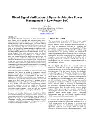
Speed Up RF Mixed-Signal Simulation Using
Novel Hierarchical Fast Envelope Simulation
Cadence Design Systems, Inc.
Qian Cai and Dan Feng
Session 6.7
Presented at

ABSTRACT
With the fast growing personal communication and electronic markets system-on-chip (SoC) and system-in-package
(SiP) circuit design has become an indispensable area in EDA. SoC integrates different types of circuits including
digital, analog, and RF contents on one chip. SiP assembles all the electronic components including digital ICs,
analog ICs, RFICs, and passive components in one package. The design of SoC and SiP requires large amount of
mixed-signal including RF simulation due to the integration of various types of functional blocks in one IC or
package. It is a big challenge to efficiently and accurately simulate mixed-signal circuits including RF blocks. It is
not only due to the different methodologies used for different blocks but also because of the complicated modulated
signals consisting of high frequency carriers and low frequency basebands often presented in the RF blocks.
Traditional transient simulation technologies are inefficient for RF signals since the time steps are limited by the
high frequency carrier and long time duration is required due to the low frequency baseband. This problem can be
solved by Cadence’s newly developed hierarchical fast envelope simulation. In this paper we present how fast
envelope simulation techniques increase the efficiency of RF mixed-signal simulation; why hierarchical approach is
important in simulating large-scale circuits; and how to use hierarchical fast envelope simulation in RF mixed-signal
simulation.
1. INTRODUCTION
As the semiconductor technology advancing into the nanometer-scale integrated circuit arena and more and more
features are built into communication and RF chips, the capacity of integrated circuits are increasing. This is also
because integration of large-scale digital logics with high performance analog/mixed signal contents onto a single
chip (SoC) has been increasingly the demand and trend of circuit designs. To increase the production yield and the
quality of the end products the circuit designers have to take into account the package circuitries during their design
phase. This leads to the demand for SiP design. Both SoC and SiP designs are very challenging especially due to
the high sensitivity of analog portion to any changes in the whole circuit. According to the manufacturers’ data, the
analog circuitry in SoC accounts for just 2 percent of the transistors and 20 percent of the area but 40 percent of the
design effort and 50 percent of the re-spins. Thus, the ability to analyze integrated circuits, including RF circuits in
wireless communications, with large capacity is becoming one of the most critical issues in SoC design.
The design of SoC and SiP requires large amount of mixed-signal including RF simulation due to the integration of
various types of functional blocks in one IC or package. Furthermore, functional failures are becoming more
common than performance failures in RF design. Verification runs using the full functionality of the chip are
becoming critical. Full-chip FastSPICE simulations for RF circuits are increasingly demanded by customers.
Digitally corrected/controlled CMOS RF is also becoming popular. It requires large numbers of verification runs
and corners. The circuit size explodes due to large functional digital blocks. Transistor level simulation is essential
since in many cases the analog and digital portions cannot be cleanly separated as behavioral blocks. In addition the
behavioral models may not be good enough or limited to some application ranges for accurate circuit simulation.
Therefore, efficient and accurate mixed-signal transistor level simulation is the key to SoC and SiP success.
RF circuits process signals generated with high frequency carriers modulated by low frequency base bands using
various schemes such as amplitude, phase and frequency modulations. The conventional transient analysis is
inefficient for RF circuit simulation due to the widely separated spectral components, which require that the time
durations follow the slow base band signals but the time steps depend on the fast carrier signals, resulting in a
prohibitively large number of time steps and very expensive computational costs. Fast envelope following
simulation is the solution to such problems and becomes the basis to first-pass successful RFIC designs.
We have developed and implemented a number of new techniques for fast envelope simulation in UltraSim and
AMS Designer. In this paper we present how to apply these new techniques in RF mixed-signal simulation to obtain
significant speed up. Fast envelope simulation techniques are described in Section 2. Hierarchical approach is
given in Section 3. Application of fast envelope simulation is demonstrated in Section 4. Examples of fast envelope
simulation are shown in Section 5. Conclusions are given in Section 6.

2.1 Overview
2. FAST ENVELOPE SIMULATION TECHNIQUES
Generally, fast envelope simulation is introduced to simulate the modulated circuits to overcome the difficulties with
conventional transient simulation where the small time steps are needed to accommodate the high frequency carrier
and long time durations are required to cover the low frequency baseband signals. These types of circuits often
appear in RF circuits such as transmitters and receivers. A typical transmitter and receiver of digital communication
are shown in Figure 1.
Figure 1. A typical RF transmitter and receiver for digital communication.
In the transmitter side the digital I and Q signals are converted by digital-to-analog converter (DAC) to analog I and
Q signals which are modulated with high frequency carrier signals. The modulated signals are amplified by the
power amplifier and then transmitted through the antenna. In the receiver side the modulated signals are received
through the antenna, amplified by the low-noise amplifier, and then demodulated back to analog I and Q signals
which are converted by analog-to-digital converter (ADC) to digital I and Q signals.
A typical modulated signal is shown in Figure 2. It clearly shows that the high frequency carrier signal is modulated
by the low frequency baseband signal. Traditional transient simulation is not efficient to simulate such signals since
large amount of time is required on simulating the details of high frequency carrier signals up to the long duration
required to cover the baseband signals.
The goal of fast envelope simulation is to obtain the low frequency baseband signal (envelope of the modulated
signal) without simulating the details of the high frequency modulated signal at each period to increase the
efficiency in simulating modulated circuits.
Figure 2. A typical modulated signal.

2.2 Simulation Techniques
Most circuit behaviors can be described by a set of N nonlinear differential algebraic equations of the form
dQ(
v(
t))
+ I(
v(
t))
+ u(
t)
= 0
dt
N
where Q( v(
t))
∈ ℜ represents contributions of the dynamic elements such as capacitors and inductors, I( v(
t))
∈ ℜ
N
is the vector representing the static elements such as resistors, u( t)
∈ ℜ is the vector of input sources, and v( t)
∈ ℜ
is the vector containing all the state variables such as node voltages and inductor currents.
Numerical schemes are usually used to solve Equation (1). Different approximations to the time-derivative
operation result in different methods such as backward and forward Euler, trapezoidal, and Gear methods.
A number of algorithms have been developed for envelope simulation. In general they can be summarized as
transient envelope following method [1, 2], modulated-oriented harmonic balance method [3-5], and Fourier
collocation method [6-8].
Transient envelope following method is a time-domain technique. There are two loops involved in solving transient
envelope following equations. The circuit envelopes are approximated by a low-order polynomial in the outer loop
allowing many cycles to be skipped, and the steady-state problem is solved in the inner loop using shooting method.
Modulated-oriented harmonic balance (HB), also referred as circuit envelope or Fourier envelope method, is a
mixed time-domain and frequency-domain technique. There are also two loops involved in the envelope analysis.
The circuit envelope is solved using the outer-loop transient analysis whose time steps are not limited by the fast
carrier signals.
Fourier collocation method is a new technique developed by Cadence for fast envelope simulation. In Fourier
collocation method the time derivatives of charges and fluxes in the nonlinear differential algebraic equations are
evaluated from the Fourier collocation points with the envelope being approximated by a low-order polynomial.
According to the characteristics of the modulated signals and the properties of the circuit Equation (1) can be solved
by envelope solve with one point per clock cycle, partial solve with a number of points per clock cycle, or full solve
with all the Fourier collocation points per cycle. An adaptive solve scheme has also been developed to increase the
simulation speed while maintain the required accuracy.
3.1 FastSPICE Tecnology
3. HIERARCHICAL APPROACH
Since the first famous circuit simulation tool SPICE developed in the early 1970’s many researches and
improvements have been done to the circuit simulation tools. In general we can classify them into two categories:
conventional SPICE and FastSPICE tools.
The conventional SPICE solves the entire circuit as a whole with compact nonlinear device models. It provides very
accurate results and is suitable for analog and mixed-signal simulation for circuits of small to medium sizes. Spectre
from Cadence, HSPICE from Synopsys and ELDO from Mentor are the typical tools for this generation. With the
fast growing circuit size of ICs the conventional SPICE simulation tools encounter speed and capacity problems
which lead to the development of the FastSPICE simulators.
The FastSPICE simulators, such as UltraSim from Cadence, NanoSim and HSim from Synopsys, apply techniques
of partition, event driven, multi-rate simulation, and simplification of device models to overcome the speed and
capacity problems of conventional SPICE. Among all these techniques partitioning is one of the most important
techniques to solve both speed and capacity problems. Partitioning divides a large design into many small partitions
which can be solved separately during simulation. Mathematically, many small matrices are solved instead of one
huge matrix. Thus much more complex designs can be handled. A simple partition is shown in Figure 3 [9].
(1)
N
N

Figure 3. A simple partition for FastSPICE simulation.
In addition to small size and less memory, partitioning makes it possible for multi-rate simulation to simulate each
partition with different time step. This is very critical in mixed-signal design since the signal change rates in each
functional block are usually very different. For example, the signals in the RF blocks change quickly due to the high
frequency carrier while the signals in the digital processing blocks change slowly since they contains only the
baseband. The multi-rate simulation can provides significant speed improvement over conventional SPICE
simulators.
3.2 Partition for Fast Envelope Simulation
In Cadence’s hierarchical fast envelope simulation any subcircuit or subcircuit instance can be designated for fast
envelope simulation. If a subcircuit is specified for fast envelope simulation any subcircuit instances using this
subcircuit will be simulated by fast envelope simulation with the same simulation options. For most efficient results
the RF blocks with high frequency carrier modulated by low frequency baseband should be specified for fast
envelope simulation. In addition to the subcircuit specified some connections or nearby subcircuits may also be
combined to form a partition for fast envelope simulation due to their strong couplings with the specified subcircuit.
Such partitioning is carried out according to the rules and algorithms implemented in UltraSim [10]. As an example
a simple digital modulation circuit is shown in Figure 4 and its RF subcircuit can be specified for fast envelope
simulation.
Figure 4. A simple digital modulation circuit.

4. APPLICATION OF FAST ENVELOPE SIMULATION
There are two major applications of fast envelope simulation in UltraSim: efficient simulation of RF modulated
circuit and speed up of normal transient simulation in the analog portion.
4.1 Simulation of RF Modulated Circuit
RF circuits usually process signals generated with high frequency carriers modulated by low frequency base bands
using various schemes such as amplitude, phase and frequency modulations. The conventional transient analysis is
inefficient for RF circuit simulation due to the widely separated spectral components, which require that the time
durations follow the slow base band signals but the time steps depend on the fast carrier signals, resulting in a
prohibitively large number of time steps and very expensive computational costs.
The main application of fast envelope simulation is to overcome the difficulties of conventional transient simulation
for RF modulated circuits and to simulate such circuits efficiently. Assuming that the frequency of the carrier is fc
and the frequency of base band signal is fb we can define a modulation ratio Mr as
f
b
M r = (9)
f c
The smaller the modulation ratio Mr the more efficient the fast envelope simulation will be. In general Mr should be
less than 0.1 in order to use fast envelope simulation meaningfully. Tipical I/Q modulated signals are shown in
Figure 5.
I
Q
Figure 5. Tipical I/Q and the composite signals from an I/Q modulator.
4.2 Speed Up Transient Simulation
Fast envelope simulation can be used to speed up normal transient simulation when there is a high frequency signal
and the details of the signal at the certain time intervals are not important such as amplifiers. The parameters
env_tstart and env_tstop can be used to specify a certain time interval for fast envelope simulation. Fast envelope
simulation will be performed in the time interval defined by env_tstart and env_tstop while normal transient
simulation will be performed at the rest of time intervals between 0 and tstop specified in the transient simulation
statement.
For example, if a circuit is simulated for the time interval between 0 and 1000ns but the most important time interval
is between 900ns and 1000ns, the fast envelope simulation can be performed from 0 to 900ns to speed up the
unimportant portion by specifying env_tstop = 900ns. The normal transient simulation will be performed right after

the fast envelope simulation is finished up to 1000ns to obtain the detail waveforms for the interval between 900ns
and 1000ns. Figure 6 shows wavforms of a circuit simulated by normal transient simulation and fast envelope
simulation with env_tstop = 900ns.
Figure 6. Waveforms obtained by normal transient simulation (the top waveform) and by fast envelope
simulation for speed up (the bottom waveform).
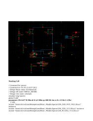
5.1 A RF Low-Noise Amplifier
5. EXAMPLES
A RF low-noise amplifier is used as the example for transient simulation speed up by fast envelope simulation. The
circuit schematic is shown in Figure 7.
Figure 7. Schematic of the low-noise amplifier.

The frequency of the RF input signal is 2.35GHz. Transient simulation time is 1μs. The responses in the transition
region are not important in this case since the designer only needs to know the steady state behavior of the amplifier.
Fast envelope simulation parameter env_tstart is set to 950ns to speed up the transient analysis. The normal
transient simulation took about 100s. The fast envelope simulation took about 7.5s. About 13x speed up is achieved
by fast envelope simulation. The RF output signals are plotted in Figure 8.
Figure 8. RF output waveforms obtained by normal transient simulation (top part) and by fast envelope
simulation (bottom part) of the low-noise amplifier.
5.2 A Simple Digital Modulation Circuit
The simple digital modulation circuit shown in Figure 9 is used to demonstrate fast envelope simulation of digital
modulated circuit.
Figure 9. A simple digital modulation circuit.
The digital signal is converted into analog signal by a DAC and multiplied by the high frequency carrier in the
modulator. The modulated signal is then demodulated in the demodulator to extract the digital signal. Normal
transient simulation took about 7.6s while fast envelope simulation took about 0.15s. About 50x speed up is
achieved by fast envelope simulation. The input signal, the modulated signal and the output signal are shown in
Figure 10. It is obvious that the output signals from both simulations are similar though the modulated signals are
quite different due to the fact that many cycles are skipped by fast envelope simulation to gain great speed up.

Figure 10. Input signal, modulated signal and output signal obtained by normal transient simulation (top
ones) and fast envelope simulation (bottom ones).
5.3 A Direct-Conversion Transmitter
A direct-conversion transmitter is shown in Figure 11. The I and Q signals are modulated with the high frequency
carrier through an I-modulator and Q-modulator. The modulated I and Q signals are combined by the adder. The
combined signal goes through an input matching circuit and then is amplified by two power amplifiers.
Figure 11. The schematic of a direct-conversion transmitter.
The circuit is simulated by both normal transient simulation and fast envelope simulation. It took about 2455s for
normal transient simulation and about 152s for fast envelope simulation to finish. Fast envelope simulation achieves
about 16x speed up. The RF output signals resulting from normal transient and fast envelope simulation are plotted
in Figure 12.

Figure 12. The RF modulated signals obtained by fast envelope simulation (top part) and normal transient
simulation (bottom part).
With option env_harms set to a value larger than 0 fast envelope simulation in UltraSim or AMS Designer can
calculate the time-varying harmonics which can be used to compute adjacent channel power ratio (ACPR) and plot
various diagrams to show the RF characteristics of the circuit. For example, power spectral density, constellation
plot and time varying harmonics are plotted in Figure 13.
(a) Power spectral density
(c) Time varying harmonics
(b) Constellation plot
Figure 13. Various plots of time varying RF characteristics.

5.4 A Compete RFIC
The RFIC shown in Figure 14 is used to demonstrate the advantages of local fast envelope simulation. The circuit is
a large-scale circuit consisting of a RF portion and a six bit ADC portion. Both the RF portion and ADC portion are
transistor level circuits.
The analog RF portion is specified for fast
envelope simulation. It consists of a RF
transmitter, a channel decay component and a RF
receiver. The transmitter performs I/Q
modulation, signal amplification and transmition.
The channel decay component models the signal
changes through the transmition channel. The
receiver carries out signal receiving, recovering
and demodulation.
The whole circuit has a total of 9596 elements and
8698 nodes. The RF portion is designated for fast
envelope simulation. The entire circuit is divided
into 191 partitions by UltraSim’s hierarchical
partition algorithm. Among them there are 164
static partitions, 26 voltage source partitions and 1
floating capacitor partition. The RF partition
consists of 2912 elements and 4584 nodes.
The circuit was simulated by local fast envelope
simulation and normal transient simulation. It
took about 1 hour and 6 minutes by local fast
envelope simulation and about 5 hours 19 minutes
by normal transient simulation. About 5x speed
up is achieved by local fast envelope simulation.
Figure 14. A complete RFIC.
The circuit is also simulated with global envelope simulation using full solve techniques. Since the entire circuit is
treated as one partition the size of the system equations to be solved is very large. It took more than 10 hours for the
global envelope simulation to finish. Figure 15 plots partial waveforms of the output signal from RF transmitter
Vt(out), output signal from RF receiver Vr(out), and digital waveform of the 6th bit output Vd(b6).
Vt(out)_nt
Vt(out)_env
Vr(out)_nt
Vr(out)_env
Vd(b6)_nt
Vd(b6)_env
Figure 15. Partial waveforms obtained by normal transient simulation (Vt(out)_nt, Vr(out)_nt, and Vd(b6)_nt)
and local envelope simulation (Vt(out)_env, Vr(out)_env, and Vd(b6)_env).

F rom this example we can see that global envelope simulation with full solve techniques is not suitable for large-scale circuits,
especially for the circuits consisting of large digital blocks and small RF portion. It shows that the local
fast envelope
simulation can significantly speeds up the RF mixed-signal simulation, especially for large-scale circuits whose RF
portion is small compared to size of the entire circuit.
5.5
Top Receiver in RF Methodology Kits
Fast envelope simulation features have also been shown in the simulation of the top receiver in the RF methodology
kits as highlighted in the schematic shown in Figure 16.
Figure 16. The top receiver in the RF methodology kits as highlighted.
The carrier frequency for the top receiver is 2.45GHz. The receiver is simulated by Spectre transient
simulation,
UltraSim
FastSPICE simulation, and local fast envelope simulations with different settings. The simulation time
comparison is shown in Table 1.
Table 1. Simulation Time Camparison

From Table 1 we can see that significant speed ups are achieved by local fast envelope simulations. The I/Q
waveforms are plotted in Figure 17. The RF data stream gets down converted and when it is ready to leave the
receiver chain we can see the bit stream of the data that goes into the digital baseband processor. As we can see
from Figure 17 the results from Spectre transient simulation and UltraSim local fast envelope simulation match very
nicely.
Figure 17. The I/Q waveforms from Spectre transient simulation (in black) and UltraSim local fast envelope
simulation (in red).
6. CONCLUSIONS
We have presented an approach to use hierarchical fast envelope simulation to speed up RF mixed-signal simulation.
The hierarchical fast envelope simulation technology integrates FastSPICE methodologies and fast envelope
simulation techniques in a single engine for efficient and accurate RF mixed-signal simulation. We have
demonstrated that fast envelope simulation can be applied to transient simulation speed up and simulation
of
modulated circuits. Fast envelope simulation can be used as a new vehicle for SoC and SiP simulation and design
to
use the most suitable technique for each functional block while maintain the required accuracy for the entire circuit.
7. ACKNOWLEDGMENTS
We would like to thank the members of Cadebce RF Methodology Kits team, especially Anand Raman, for
providing information and materials of the RF methodology kits which are presented in this paper.

8. REFERENCES
[1] Petzold, L., “An Efficient Numerical Method for Highly Oscillatory Ordinary Differential Equations”, SIAM J.
Numer. Anal., Vol. 18, pp. 455-479, June 1981.
[2] Kundert, K., White, J. and Sangiovanni-Vincentelli, A., “An Evelop-Following Method for the Efficient
Transient Simulation of Switching Power and Filter Circuits”, IEEE Int. Conf. Computer-Aided Design Dig.
Tech. Papers, November, 1998.
[3]
Sharrit, D., “New Method of Analysis of Communication Systems,” Proc. MTTS’96 WMFA: Nonlinear CAD
Workshop, June, 1996.
[4] Rizzoli, V., Neri, A. and Mastri, F., “A Modulated-Oriented Piecewise Harmonic-Balance Technique Suitable
for Transient Analysis and Digitally Modulated Signals,” Proc. 26
Feldmann, P. and Roychowdhury, J., “Computation of Circuit Waveform Envelopes Using an Efficient, Matrix-
Decomposed Harmonic Balance Algorithm”, IEEE Int. Conf. Computer-Aided Design Dig. Tech. Papers,
November, 1996.
[6] Baolin Yang and Qian Cai, “A Novel Approach for Fast Envelope Following Simulation Using Fourier
Collocation Method”, Proc. CTC 2004.
[7] Baolin Yang, Qian Cai and Bruce W. McGaughy, “A Robust Adaptive Solve Scheme for Fast Envelope
Following Transient Simulation”, Proc. CTC 2005.
[8] Qian Cai, Dan Feng, Bruce McGaughy, Daniel Liu, Rendong Lin, Fangyi Rao, Vincent Li, and Yuchun Deng,
“Integrated Analog Mixed-Signal Simulation for RFIC Design Flow”, Proc. CTC 2006.
[9] Stefan Wuensche, Bruce McGaughy, Jun Kong, Peter Frey, Baolin Yang, and Jaideep Mukherjee, “Using Hierarchy and
Isomorphism to Accelerate Circuit Simulation”, ICU 2003.
[10] UltraSim User’s Manual, Cadence Design Systems, Inc.
th Microwave Conf., Prague, Czech Republic,
September, 1996. pp. 546-550.
[5]