Non-dispersive wave packets in periodically driven quantum systems

|ψ (z)| 2
|ψ (z)| 2
0.3
0.2
0.1
0.0
0.3
0.2
0.1
A. Buchleitner et al. / Physics Reports 368 (2002) 409–547 505
0.0
0 100 200 0 100 200
z z
|Tunneling splitting|
10 0
10 -5
10 -10
10 -4
10 -9
10 -14
0.0 0.1 0.2 0.3
λ
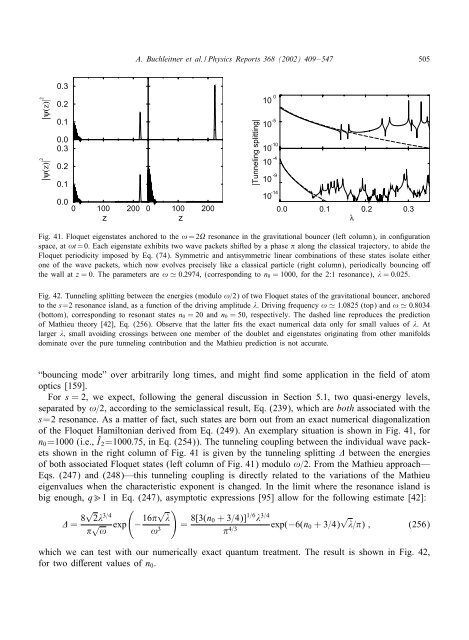
Fig. 41. Floquet eigenstates anchored to the ! =2 resonance in the gravitational bouncer (left column), in con guration
space, at !t =0. Each eigenstate exhibits two wave packets shifted by a phase along the classical trajectory, to abide the
Floquet periodicity imposed by Eq. (74). Symmetric and antisymmetric linear combinations of these states isolate either
one of the wave packets, which now evolves precisely like a classical particle (right column), periodically bouncing o
the wall at z = 0. The parameters are ! 0:2974, (corresponding to n0 = 1000, for the 2:1 resonance), =0:025.
Fig. 42. Tunneling splitting between the energies (modulo !=2) of two Floquet states of the gravitational bouncer, anchored
to the s=2 resonance island, as a function of the driving amplitude . Driving frequency ! 1:0825 (top) and ! 0:8034
(bottom), corresponding to resonant states n0 = 20 and n0 = 50, respectively. The dashed line reproduces the prediction
of Mathieu theory [42], Eq. (256). Observe that the latter ts the exact numerical data only for small values of .At
larger ; small avoiding crossings between one member of the doublet and eigenstates originating from other manifolds
dominate over the pure tunneling contribution and the Mathieu prediction is not accurate.
“bouncing mode” over arbitrarily long times, and might nd some application in the eld of atom
optics [159].
For s = 2, we expect, following the general discussion in Section 5.1, two quasi-energy levels,
separated by !=2, according to the semiclassical result, Eq. (239), which are both associated with the
s=2 resonance. As a matter of fact, such states are born out from an exact numerical diagonalization
of the Floquet Hamiltonian derived from Eq. (249). An exemplary situation is shown in Fig. 41, for
n0=1000 (i.e., Î 2=1000:75, in Eq. (254)). The tunneling coupling between the individual wave packets
shown in the right column of Fig. 41 is given by the tunneling splitting between the energies
of both associated Floquet states (left column of Fig. 41) modulo !=2. From the Mathieu approach—
Eqs. (247) and (248)—this tunneling coupling is directly related to the variations of the Mathieu
eigenvalues when the characteristic exponent is changed. In the limit where the resonance island is
big enough, q1 in Eq. (247), asymptotic expressions [95] allow for the following estimate [42]:
= 8√ 2 3=4
√ ! exp
√
16
−
! 3
= 8[3(n0
1=6 3=4
+3=4)]
exp(−6(n0 +3=4) 4=3 √ = ) ; (256)
which we can test with our numerically exact quantum treatment. The result is shown in Fig. 42,
for two di erent values of n0.