The Bak–Tang–Wiesenfeld „sandpile“ model (1987)

The Bak–Tang–Wiesenfeld
„sandpile“ model (1987)
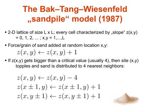
• 2-D lattice of size L x L; every cell characterized by „slope“ z(x,y)
= 0, 1, 2, ... ; x,y = 1,...,L
• Force/grain of sand added at random location x,y:
z(x, y) ← z(x, y)+1
• If z(x,y) gets bigger than a critical value (usually 4), then site (x,y)
topples and sand is distributed to 4 nearest neighbors:
z(x, y) ← z(x, y) − 4
z(x ± 1,y) ← z(x ± 1,y)+1
z(x, y ± 1) ← z(x, y ± 1) + 1

Avalanches in the BTW
„sandpile“ model
Toppling of one site can lead to one or more neighboring sites
toppling, whose neighbors may topple, etc.: avalanches.
Question: what should happen at the boundary?
- sand falls off the edge or
- sand is conserved.
An avalanche has a size (how many sites topple?) and a duration.
What is the distribution of avalanche sizes and durations?

Self-Organized Critical Model
Example:
[Bak, Tang, Wiesenfeld, 1987
15.04.2012 Viola Priesemann Neuronal Avalanches
9

Bak, Tang, Wiesenfeld (1987)

Interestingly, the distributions of avalanche sizes and durations
have power laws.
p(s) ∝ s −αs , αs ≈ 5/4
p(t) ∝ t −αt , αt ≈ 3/4
In physical systems, such power laws are often associated with
phase transisitons and occur only at finely tuned parameter
settings of, e.g., the temperature. Here, the systems tunes itself
to critical behavior. This is why this is called self-organized
criticality (SOC).
Similar power laws are observed in many different contexts ranging
from the distributions of earth quakes over volcanic activities
and brain activity to stock market crashes and many others.
Some of these phenomena may also be instances of SOC.

P(x)
P(x)
P(x)
P(x)
10 0
10 !1
10 !2
10 !3
10 !4
10 !5
10 0
10 !1
10 !2
10 !3
10 !4
10 !5
10 0
10 !1
10 !2
10 !3
10 !4
10 !5
10 0
10 !1
10 !2
10 !3
10 0
10 0
10 0
10 0
10 2
10 4
(a)
10 0
10 !1
10 !2
10 !4
10 !3
words proteins
Internet
10 2
terrorism
10 2
10 2
x
10 4
(d)
(g)
(j)
10 4
10 4
10 6
10 0
10 !2
10 !4
10 !6
10 0
10 !2
10 !4
10 !6
10 0
10 !1
10 !2
10 0
10 0
10 2
10 3
10 4
calls
10 2
10 4
10 1
HTTP
10 5
10 4
10 6
10 6
(b)
(e)
(h)
10 2
10 6
10 8
10 7
10 0
10 !2
10 !4
10 0
10 !1
10 !2
10 0
10 !1
10 !2
10 !3
10 0
10 0
10 0
metabolic
10 1
wars
10 1
species
10 !3
10 !3
birds blackouts book sales
x
(k)
10 0
10 !1
10 !2
10 6
10 1
x
10 2
10 2
10 7
(c)
(f)
(i)
(l)
10 3
10 3
10 2
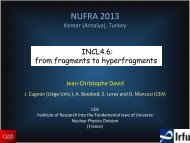
Power-law distributions in empirical data 25
Clauset, Shalizi, Newman (2009). Power-law distributions in empirical data
Fig. 6.1. The cumulative distribution functions P (x) and their maximum likelihood power-law Fig. 6.2. The cumulative distribution functions P (x) and their maximum likelihood power-law
fits for the first twelve of our twenty-four empirical data sets. (a) The frequency of occurrence of fits for the second twelve of our twenty-four empirical data sets. (m) The populations of cities
unique words in the novel Moby Dick by Herman Melville. (b) The degreedistributionofproteinsinin
the United States. (n) The sizes of email address books at a university. (o) The number of
the protein Power interaction network law of the yeast distributions S. cerevisiae. (c) The degree distribution are ofubiquitious. metabolitesacres
burned in California But forest fires. there (p) The intensities could of solarbe flares. (q) The intensities of
in the metabolic network of the bacterium E. coli. (d) The degree distribution of autonomous systems earthquakes. (r) The numbers of adherents of religious sects. (s) The frequencies of surnames in
(groups of computers under single administrative control) on the Internet. (e) The number of callsthe
United States. (t) The net worth in US dollars of the richest people in America. (u) The
received by many US customers different of the long-distance telephone mechanisms carrier AT&T. (f) The intensity responsible of warsnumbers
of citations received for by published them academic - papers. not (v) just The numbers SOC.
of papers authored
from 1816–1980 measured as the number of battle deaths per 10 000 of the combined populations of by mathematicians. (w) The numbers of hits on web sites from AOL users. (x) The numbers of
the warring nations. (g) The severity of terrorist attacks worldwide from February 1968 to Junehyperlinks
to web sites.
2006, measured by number of deaths. (h) The number of bytes of data received in response to HTTP
(web) requests from computers at a large research laboratory. (i) The number of species per genus
of mammals during the late Quaternary period. (j) The frequency of sightings of bird species in the the alternatives we tested using the likelihood ratio test, implying that these data sets
United States. (k) The number of customers affected by electrical blackouts in the United States.
(l) The sales volume of bestselling books in the United States.
are not well-characterized by any of the functional forms considered here.)
Tables 6.2 and 6.3 show the results of likelihood ratio tests comparing the best fit
P(x)
P(x)
P(x)
P(x)
10 0
10 !1
10 !2
10 !3
10 !4
10 !5
10 0
10 !1
10 !2
10 !3
10 0
10 2
10 4
10 6
(m)
10 !4
10 !3
10 !6
cities email fires
(p)
10 8
10 1 10 2 10 3 10 4 10 5 10 6
10 !5
10 !4
flares
10 0
10 !1
10 !2
10 !3
10 !4
10 4
10 !3
10 !2
10 !1
10 0
10 !4
10 0
10 !6
10 !5
surnames
10 5
authors
10 1
x
10 2
10 6
(s)
(v)
10 3
10 7
10 0
10 !1
10 !2
10 0
10 !1
10 !2
10 !3
10 !4
10 !5
10 0
10 !1
10 !2
10 !3
10 0
10 0
10 0
10 8
10 !5
10 !4
10 !3
10 !2
10 !1
10 2
10 1
quakes
10 9
10 4
wealth
web hits
10 2
10 6
10 10
(n)
(q)
(t)
10 3
10 8
10 11
(w)
10 0 10 1 10 2 10 3 10 4 10 5
x
10 !5
10 !4
10 !3
10 !2
10 !1
10 0
10 0
10 !1
10 !2
10 0
10 6
10 0
10 !6
10 !5
10 !4
10 !3
10 !2
10 !1
10 0
10 0
10 !2
10 !4
10 !6
10 !8
10 !10
10 0
10 1
10 2
religions
10 7
citations
10 2
10 2
web links
x
10 4
10 4
10 8
10 3
(o)
(r)
(u)
(x)
10 6
10 6
10 9
10 4

Branching Processes
Following Grinstead & Snell, Introduction to Probability
Simple statistical model with many applications in, e.g., population
dynamics, propagation of activity in the nervous system, nuclear
chain reactions, ...
In sand pile model, one toppling site (parent) may induce toppling
in other sites (children), which can induce further toppling in
even more sites (grandchildren).
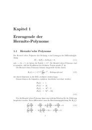
Here: always start with one individual. This individual creates
0,1,2,3,... offspring with probability: p0,p1,p2,p3,...
In the next generation, each offspring independently has the same
probabilities of creating their own offspring.

Here: always start with one individual. This individual has a certain
probability of creating 0,1,2,3,... offspring. In the next generation,
each offspring independently has the same probability of
creating further offspring.
378 CHAPTER 10. GENERATING FUNCTIONS
Example:
1/4
1/4
1/2
2
1
0
1/2
1/16
1/8
5/16
Figure 10.1: Tree diagram for Example 10.8.
What is the probability of having a certain number of offspring
in a certain generation? What is the probability of extinction?
Branching processes have served not only as crude models for population growth
but also as models for certain physical processes such as chemical and nuclear chain
1/4
1/4
1/4
1/4
1/2
4
3
2
1
0
2
1
0
1/64
1/32
5/64
1/16
1/16
1/16
1/16
1/8

CHING PROCESSES 379
Probability that process dies out by the mth generation:
the probability that the process dies out by the mth generation. Of
For the example calculate:
0. In our example, d1 =1/2 and d2 =1/2+1/8+1/16 = 11/16 (see
Note that:
d0,d1,d2
Note that we must add the probabilities for all paths that lead to 0
eneration. It is clear from the definition that
0=d0 ≤ d1 ≤ d2 ≤ ···≤ 1 .
nverges to a limit d, 0≤ d ≤ 1, and d is the probability that the
ltimately die out. It is this value that we wish to determine. We
ressing the value dm in terms of all possible outcomes on the first
f there Thus, are the jsequence offspringconverges in the first to generation, a value: 0 ≤then d ≤ 1to
die out by the
on, each of these lines must die out in m − 1 generations. Since they
How can we calculate d?
endently, this probability is (dm−1) j . Therefore
See blackboard.
dm = p0 + p1dm−1 + p2(dm−1) 2 + p3(dm−1) 3 + ··· . (10.1)
he ordinary generating function for the pi:
dm

This leads us to the following theorem. ✷
Theorem 10.2 Consider a branching process with generating function h(z) for the
number of offspring of a given parent. Let d be the smallest root of the equation
z = h(z). If the mean number m of offspring produced by a single parent is ≤ 1,
then d = 1 and the process dies out with probability 1. If m>1 then d