Steady State and Transient Short Circuit Analysis of 2x25 kV ... - UIC

Steady State and Transient Short Circuit Analysis of 2x25 kV High Speed Railways
Abstract
1 L. Battistelli, M. Pagano D.Proto, 2 A. Amendola, L. Cundurro, A. Pignotti
Università degli Studi di Napoli Federico II, Napoli, Italy 1 ;
Ansaldo Segnalamento Ferroviario,Napoli, Italy 2
In the paper, a detailed model for the short circuit analysis of the AC 2x25 kV-50 Hz traction
system has been derived and implemented. Two different methods have been used: the time
domain and frequency domain approaches. The two approaches are discussed and numerical
applications are reported. In particular, in order to assess the feasibility of both the two
methodologies, the results have been compared in steady state condition. Then a transient
analysis has been performed by means of the time domain simulator evidencing the short circuit
current transient behavior.
Introduction
The 2x25 kV feeding system is considered an optimal solution for high speed railways. The
reduction in the number of electric substations as well as a greater efficiency due to the use of
higher transmission voltages (50 kV supply between catenary and return feeder) with lower
currents and lower voltage locomotive traction equipment (25 kV rail-catenary voltage) are the
main advantages of the system [1]. Moreover, other advantages are related to the reduction of
electromagnetic interference between traction converters and adjacent telecommunications
circuits as well as the reduction of voltage drops.
Notwithstanding, critical operating conditions related to short circuit events can occur interfering
with the traction system components so compromising the functionality of the whole system.
The short circuit levels are particularly critical also due to the presence of the autotransformers
that increases the fault currents. Short-circuit analysis is important not only for determining the
rating of power equipment and the setting of protection devices but also for checking the voltage
profiles of the network and of the buses near the fault as well as the electromagnetic
compatibility with adjacent circuits. Thus, a detailed short-circuit study is required in both steady
state and transient condition [2-3].
The accuracy of the system components is an important concern for the short circuit analysis
since it significantly affects the simulation results. A critical issue, for example, is the
identification of the impedances of the system components and the configuration of the network
since they mainly determine the short-circuit results. Particular attention must be paid to an
accurate modeling of the autotransformers as well as of both self and mutual impedances of the
contact wire, rails and feeder.
In this paper the 2x25 kV electric railway system has been modeled in order to perform detailed
steady state and transient short-circuit analyses. The steady state model has been implemented
by means of a sequence of impedance matrices (chain matrices) representing each component
[4-5].
The same system has been implemented also by using computer simulations developed in time
domain by means of Matlab Power System Blockset, allowing to easily evaluate complex
system behavior by representing each power system component by an equivalent block. The
toolbox is suitable for efficient time-domain simulations, allowing to capture the functional
dependence of system characteristics on time and various interest parameters. Through the
time domain simulation, the short circuit analysis has been performed in transient condition.
In the paper the description of the considered traction system and of the problem formulation as
well as the description of both the two proposed methodologies has been detailed. Both steady
state and transient conditions have been investigated. Some experimental results on a
measurement campaign conducted on the actual Italian system validate the results obtained in
the simulation procedure.

Problem Description
In the 2x25 kV traction system the substation transformer feeds the overhead contact wire that
supplies the trains as well as the feeder wire that runs along the track. The voltage of the
overhead contact wire and feeder are respectively +25 kV and -25 kV. Autotransformers spaced
along a section of track connect the contact wire, feeder and rails through a median tap. The
electrical substations are equipped with 2 single phase transformers, each one feeding a railway
line section of about 25 km. Autotransformers distanced by approximately 12 km divide the line
sections in cells. In this configuration the current flows through the contact line and the feeder
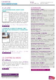
and there is no current in the rails except in the cell occupied by the train. The simplified
scheme of the system operating condition (100 A traction load) is shown in Fig.1.
- 25 kV FEEDER
50A
50A 50A
+ 25 kV CONTACT WIRE
1 st cell
50A
50A
25A
25A
2 nd cell 3 rd cell
25A
50A
Fig.1: 2x25 kV traction system scheme
A 12 km cell contains all the basic elements constituting the 2x25 kV traction system:
- the substation equipped with two single phase 60 MVA transformers;
- the parallel post (PP) equipped with two single phase 15 MVA autotransformers;
- the supply circuit containing messenger wires, contact lines, feeders and rails;
- the earth circuit containing the protection and buried earth conductors.
- capacitive compensators, located between the rails every 100 m;
- inductive bonds, connecting the rails to the earth circuit for interference mitigation, located
every 1500 m.
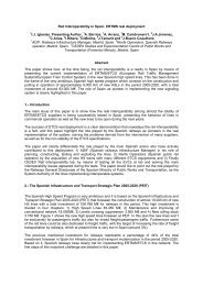
The transversal section of Fig.2 shows 14 conductors: the double track system wires (2 contact
lines, 2 feeders, 2 messenger wires, 4 rail tracks, 2 buried earth conductors, 2 overhead earth
conductors).
Two alternative implementations have been considered for short-circuit analysis. The former is
performed by means of the frequency domain algorithm. The latter is performed by means of
time domain simulation.
Feeder
Protection
wire
Messenger wire
Contact wire
Contact wire
Rails Rails
Buried earth wires
Messenger wire
Feeder
Protection
wire
Fig.2: Transversal section of the 2x25 kV railway system.
To perform the analyses in the frequency domain, each element is represented by means of an
equivalent impedance matrix. The system is solved by means of algebraic matrix operations.

In the time domain simulation, each component is represented by its differential equations.
Finally, the system is represented by the whole set of the differential equations.
In the following the system modeling for both the two approaches is briefly discussed [6].
Solving Procedures
Frequency domain model This algorithm starts representing the traction system by the node
impedance matrix through inspection and, then, it deduces the fault current in each branch of
the traction network as well as the curve of fault current versus fault location. The algorithm has
the following advantages:
- all system components are described in exactly the same manner by defining their "primitive
Z-node matrix";
- some more complex cases that often require "approximations" in classical methods can be
handled in a clean manner without numerical difficulties.
The basic idea of the frequency domain model is the representation of the whole system
through a sequence of impedance matrices (chain matrices) representing each component.
According to the aim of the approach, each element is represented by a chain matrix, which
relates the output voltages and currents to the input values:
⎡V
⎢
⎣I
out
out
⎤
⎥ =
⎦
⎡V
⎤
⎡A
in 1 2 in
[ A]
⋅ ⎢ ⎥ = ⎢ ⎥ ⋅ ⎢ ⎥
⎣I
in ⎦ A 3 A 4 ⎣I
in ⎦
⎣
A ⎤ ⎡V
⎤
⎦
where Vout (Iout) is the [nx1] output voltage (current) vector, Vinp (Iinp) is the [nx1] input voltage
(current) vector, and A is the [2nx2n] chain matrix. Matrix A can be divided in four submatrices
of [nxn], where, in particular, A2 is the impedance matrix, and A3 is the admittance matrix.
Chain matrices can be calculated as the product of the matrices of each individuated element.
Aim of the model is the identification of voltage and current phasors at all the system locations.
It is worth noting that the model of the system components significantly affects the level of
accuracy of the simulations.
In the following a description of each component’s frequency domain model is detailed.
Substation model. The substation model is basically constituted by the single phase
transformer and the substation earth circuit. Fig.4 shows the equivalent circuit model adopted
for the substation transformer.
VS
RT
Z1
Fig.4: Substation equivalent circuit
Z2
Z3
Messanger
wires
Contact
wires
Feeders
Buried and
overhead
earth
conductors
For this representation 14 equivalent circuit equations and the corresponding matrix equation
have been derived:
[ V( 0)
] [ V ] − [ Z ] ⋅[
I(
0)
]
= S
s (2)
The substation model is represented by a [14x1] matrix. VS assumes value of +25kV for
messenger and contact wires, -25kV for feeder; ZS is derived from the equivalent circuit of the
figure.
Rails
(1)

Parallel post model. The parallel post is constituted by the autotransformer whose equivalent
circuit is shown in Fig.5. The characteristic chain matrix is:
[ V( x) ] [ Zpp
] ⋅[
I(
x)
]
= (3)
where ZPP is derived from the equivalent circuit of Fig.5.
Messanger
wires
Contact
wires
Buried and
overhead
earth
conductors
Rails
Feeders
ZT
Zm
Fig.5: Parallel Post equivalent circuit
Z1
Z2
Messanger
wires
Contact
wires
Buried and
overhead
earth
conductors
Multi-conductor line model. The line section is modeled according to the method proposed in
[7]. The model includes 14 conductors whose auto and mutual impedances have been
considered. The governing multi transmission line (MTL) equations are a coupled set of firstorder
partial differential equations:
∂
∂
V(
z,
t)
= RI(
z,
t)
− L I(
z,
t)
∂z
∂z
∂
∂
I(
z,
t)
= GV(
z,
t)
− C V(
z,
t)
∂z
∂z
where V contains the line voltages with respect to the reference conductor; I contains the line
currents; and R, L, G, and C denote the per-unit-length parameters. The parameters are
calculated from the geometry of the multi-conductor line configuration and the physical
characteristics of the conductors.
The solution of the general phasor MTL equations for a line of length A can be written in the
chain matrix form as:
⎡V(
A)
⎤ ⎡Θ
⎢ ⎥ = ⎢
⎣ I(
A)
⎦ ⎣Θ
11
21
( A)
( A)
Θ
Θ
12
22
( A)
⎤ ⎡V(
0)
⎤
⎥ ⋅
( A)
⎢ ⎥
⎦ ⎣ I(
0)
⎦
Signalling track circuit element model. Two main components have to be considered for an
accurate modelling of the system behaviour: the capacitive compensators and the inductive
bonds.
a) Capacitive compensator
The chain sub-matrices of the element are calculated by output-input relations derived
according to the circuit of Fig.7:
⎡V1C
⎤ ⎡I
1C ⎤ ⎡A
C1 AC
2 ⎤ ⎡I1C
⎤
⎢ ⎥ = [ A ] ⋅ ⎢ ⎥ = ⎢ ⎥ ⋅ ⎢ ⎥ (6)
C
⎣V2C
⎦ ⎣I
2C
⎦ ⎣A
C3
AC
4 ⎦ ⎣I
2C
⎦
where [AC1]= [AC4]=[I], [AC4]=0 and
Rails
Feeders
(4)
(5)

[ A ] &
C3
⎡0
⎢
⎢
0
⎢..
⎢
⎢0
= ⎢..
⎢
⎢0
⎢..
⎢
⎢0
⎢
⎣0
0
0
..
0
..
0
..
0
0
..
..
..
..
..
..
..
..
..
0
0
..
− jωC
..
jωC
..
0
0
..
..
..
..
..
..
..
..
..
0
0
..
jωC
..
− jωC
..
0
0
⎡V1C
⎤
⎢ ⎥
⎣ I1C
⎦
..
..
..
..
..
..
..
..
..
0
0
..
0
..
0
..
0
0
0⎤
0
⎥
⎥
.. ⎥
⎥
0⎥
.. ⎥
⎥
0⎥
.. ⎥
⎥
0⎥
0
⎥
⎦
.
.
.
C
Fig.7: Compensator capacitor
b) Inductive bond
Similarly, the chain submatrices of the inductive bond are calculated by output-input relations
derived according to the circuit of Fig.8.
.
.
.
L
L
rail
rail
Earth conductors
⎡V2C
⎤
⎢ ⎥
⎣ I2C
⎦
⎡V
1i
⎤
⎡V
2i
⎤
⎢ ⎥
⎣ I
⎢ ⎥
1i
⎦
⎣ I 2i
⎦
rails
rails
Earth conductors
Fig.8: Inductive bonds
Time domain model. The time domain simulations are developed by means of Matlab Power
System Blockset (PSB). Each component is represented by a block, suitable to physically
represent the behaviour of the component.
In the following the description of each component’s time domain model is detailed.
Substation model. The substation model is a 14 output line block basically composed by a
single phase three windings transformer whose secondary windings are connected to feeders,
contact wires and rails, Fig.9.
AC
SSE 60 MVA, 50 kV
RT
Fe 1
1
2
Fe 2
3
FP 1
4
LDC1
5
FP 2
6
LDC 2
7
rot ext 1
8
rot int 1
9
rot int 2
10
rot ext 2
11
Cdt 1
12
Disp 1
13
Cdt 2
14
Disp 2
Fig.9: PSB Substation model

Parallel post model. For the autotransformer model, a 14 I/O line block composed by a single
phase three windings transformer connected as represented in Fig.10 has been used.
Fig.10: PSB parallel post model
Multi-conductor line model. The multi-conductor line has been implemented by the PSB
Distributed Parameters Line Block, that implements a N-phase distributed parameter line model
with lumped losses. The resistance R, inductance L, capacitance C line parameters are
specified in [nxn] matrices.
Signalling track circuit elements model. To reproduce the effects of capacitive compensators
and inductive bonds, equivalent electrical lumped elements have been introduced in the model,
according to the data reported in Tab.1.
Capacitive compensator (rail to rail) 25e-6 F
Inductive bond (rail to buried earth
conductor)
1.2 mH
Table 1: Capacitive compensator and inductive bond values.
It can be noted that the time domain model allows to perform analyses in both steady state and
transient conditions. The frequency domain model is an optimal tool for performing steady state
analysis and is particularly suitable for harmonic studies [7,8]. It can be also used to analyze
transients subject to the limitations of the superposition principle (applicable to linear systems).
In the current paper the following assumptions have been made:
- According to the technical literature [8,9], the electromagnetic fields have TEM structure,
which corresponds to the assumption of planewave propagation along the line.
- The multi conductor line representation does not take into account the inequalities in the
earth’s surface and its lack of conductive homogeneity whose estimation can be found in [10]
- According to [11], for short circuit analyses, the lumped compensator capacitors have been
neglected.
Numerical Applications
In order to test the two implemented simulation methods for the short circuit analysis, several
system configurations have been considered. In the following the results obtained for two
system configurations: a single cell of 12 km and a 4-cell system of about 50 km.
The first case implemented consists of a short circuit (between the overhead catenary and rail)
located at 0.7 km far from the substation. The single cell is included between the substation and
the parallel post. The short circuit has been simulated with a resistance of 0.001 Ω. Tab. I
shows the numerical results in steady state conditions.

Monitored RMS
values
[A]
Distances from
the substation
[km]
Time
Domain
Frequency
domain
If 0.7 9973 9597
Icl 12 936.7 844.7
Ife 12 924.1 868.3
Irail 12 414.6 473.2
Icl 0 9036 8753
Ife 0 923.5 867.7
Irail 0 6652 7518
Table 2: Comparison of the results of the steady state short circuit analysis [6]
Tab. 2 evidences that the two models give similar results. A slightly higher fault current can be
observed in the time domain simulation.
In order to test the system in transient condition a 50 km traction system has been considered.
The system of 4 cells includes 1 feeding substation and 4 parallel posts. The short circuit is
located at the distance of 50 km from the substation in correspondence of the fourth parallel
post. The short circuit occurs at 0.5 ms between overhead and buried earth wires.
Fig. 11 shows the instantaneous waveform of the peak fault current.
Fig. 11: Waveform of the fault current in case of overhead-buried earth wire short circuit
By the analysis of the figure it can be noted that the system is characterized by a typical first
order dynamic where the peak value depends on the instantaneous system conditions when the
short circuit occurs. The time constant is a function of the system parameters and for severe
short circuit it very slightly depends on the short circuit resistance value. To focus on the
transient in Fig. 12 the positive peak values of the fault current are reported.

Conclusions
Fig. 12: Positive fault current peak values
Two methodologies for short circuit current calculation in the 2x25 kV traction system have been
proposed. The two approaches are performed in frequency and time domains. They both
represent the physical components by means of respectively the chain matrix and partial
differential equation mathematical models.
The numerical application reported investigates on steady state and transient operating
conditions. The results of the application are able to assess the suitability to perform short circuit
analyses by both the two models.
Future works will be aimed at validating the numerical applications with experimental results
obtained through a measurement campaign.
References
[1] I. Senol, H. Gorgun, M.G. Aydeniz: “General comparison of the electrical transportation
systems that are fed with 1×25 kV or 2×25 kV and expectations from these systems”,
Electrotechnical Conference, 1998 MELECON 98, 9th Mediterranean, Vol.2, 18-20 May 1998
Page(s): 885 – 887.
[2] T. H. Chen, Y. F. Hsu, “Systematized short-circuit analysis of a 2x25 kV electric traction
network”, Electric Power Systems Research, Vol. 47, 1998, pp. 133-142.
[3] P.C. Coles, M. Fracchia, R.J. Hill, P. Pozzobon, A. Szelag: “Identification of catenary
harmonics in 3 kV DC railway traction systems”, Proceedings of the 7th Mediterranean
Electrotechnical Conference, Vol. 2, April 1994, pp. 825 -828.
[4] Clayton R. Paul: “Analysis of Multiconductor Transmission Lines”, John Wiley & Sons,
November 2007.
[5] J. Arillaga, N.R. Watson, S. Chen: “Power System Quality Assessment”, John Wiley and
Sons, 2000 pp.171-228.
[6] A. Amendola, L.Battistelli, L.Cundurro, M.Pagano, D.Proto: “Short Circuit Modelling and
Simulation of 2x25 kV High Speed Railways”, accepted to the 10 th International Confeence on
Computer Modelling and Simulation, 1-3 April 2008.
[7] R. Cella, G. Giangaspero, A. Mariscotti, A. Montepagano, P. Pozzobon, M. Ruscelli, and M.
Vanti: “Measurement of AT Electric Railway System Currents at Power-Supply Frequency and

Validation of a Multiconductor Transmission-Line Model”, IEEE Transactions on Power Delivery,
Vol. 21, N.3, 2006, pp. 1721-1726.
[8] A. Mariscotti, P. Pozzobon: “Determination of the electrical parameters of railway traction
lines: Calculation, measurement and reference data”, IEEE Trans. Power Del., vol. 19, no. 4,
Oct. 2004, pp. 1538–1546.
[9] R.J. Hill, D.C. Carpenter: “Rail track distributed transmission line impedance and admittance:
theoretical modeling and experimental results”, IEEE Transactions on Vehicular Technology,
Vol. 42, Issue 2, May 1993, pp. 225 -241.
[10] J.R.Carson: “Wave propagation in overhead wires with ground return”, The Bell System
Technical Journal, Vol. 5, 1926, pp. 539-544.
[11] CEI EN 60909-0, “Correnti di cortocircuito nei sistemi trifasi in corrente alternata”, 2001-12.
Appendix
The results reported are obtained for following parameters of the traction system:
Substation transformer parameters
Power: 60 MVA, voltage ratio: 132/2x27.5 kV, short circuit voltage: 10%
Auto-transformer Parameters
Power: 15 MVA, voltage ratio: 27.5/0/-27.5 kV, short circuit voltage: 1%.
Multi conductor line parameters
Tab. A shows the materials, resistivity (Ω/km), sections and positions of all the conductors
involved in the systems.
Description Material Resistance Section
[Ω/km] [mm 2 ]
X
[m]
Y
[m]
Left side track system
Feeder Al 0,109 307 -6,60 8,00
Messanger Cu 0,15 120 -2,50 6,55
Contact line Cu 0,12 150 -2,50 5,30
External Rail UNI60 -3,26 0,01
Internal Rail UNI60 -1,74 0,01
Buried earth wire Cu 0,19 95 -5,00 -1,12
Protection wire Al 0,225 150 -6,12 5,50
Right side track system
Feeder Al 0,109 307 6,60 8,00
Messanger Cu 0,15 120 2,50 6,55
Contact line Cu 0,12 150 2,50 5,30
External Rail UNI60 3,26 0,01
Internal Rail UNI60 1,74 0,01
Buried earth wire Cu 0,19 95 5,00 -1,12
Protection wire Al 0,225 150 6,12 5,50
Table A: Track line parameters