THE SMOOTH SOUNDING GRAPH. A Manual for Field Work ... - BGR
THE SMOOTH SOUNDING GRAPH. A Manual for Field Work ... - BGR
THE SMOOTH SOUNDING GRAPH. A Manual for Field Work ... - BGR

Create successful ePaper yourself
Turn your PDF publications into a flip-book with our unique Google optimized e-Paper software.
25<br />
curves have to be calculated theoretically. Just <strong>for</strong> instruction the 2-layer<br />
ρa master curves are shown in Fig.17. Here the values are plotted as<br />
ρ1<br />
L / 2<br />
functions <strong>for</strong> different ratios µ of the resistivities of the two layers.<br />
h<br />
2-layer master curves were available be<strong>for</strong>e 1930. In 1933-36 CGG<br />
(Compagnie Generale de Geophysique), Paris, calculated 3-layer master<br />
curves. Since 1955 master curves <strong>for</strong> any number of layers can be pro-<br />
vided. Nowadays within a few seconds by electronic computers.<br />
But the interpretation does not belong to the scheme of this manual. We<br />
there<strong>for</strong>e continue keeping in mind that a sounding graph has to be<br />
smooth in order to guarantee a quantitative interpretation.<br />
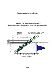
depth [m] resistivity [Ωm]<br />
0-2<br />
2-6<br />
6-26<br />
26-<br />
100<br />
2000<br />
10<br />
100<br />
overburden<br />
dry sand<br />
clay<br />
aquifer (fresh water)<br />
Let us add some remarks <strong>for</strong> better understanding the zooming process.<br />
This shall be done by discussing a 4-layer case very often occuring in hy-<br />
drogeological prospecting <strong>for</strong> groundwater. The layer sequence is given in<br />
Fig.18 in logarithmic scale.<br />
Observing the current density j between M and N<br />
at the surface the high resistant second layer will<br />
increase j at the beginning of the zooming process<br />
quite simitar to the simple 2-layer example in<br />
Fig.12-14. The current lines are pushed onto the<br />
surface. Continuing the process, however, the well<br />
conducting third layer will collect the current lines<br />
(pull them downwards) thus causing a decrease of<br />
j at the surface. Finally the aquifer, i.e. the fourth<br />
layer (100Ωm) will push again the current up-<br />
wards.<br />
Fig.18