THE SMOOTH SOUNDING GRAPH. A Manual for Field Work ... - BGR
THE SMOOTH SOUNDING GRAPH. A Manual for Field Work ... - BGR
THE SMOOTH SOUNDING GRAPH. A Manual for Field Work ... - BGR

You also want an ePaper? Increase the reach of your titles
YUMPU automatically turns print PDFs into web optimized ePapers that Google loves.
with just the same factor K.<br />
22<br />
After this we now return to our two-layer case discussed by aid of Fig.12-<br />
15 and shall proceed to plot the result in a diagram. i.e. we want to con-<br />
struct a "sounding graph" ρa( L<br />
2 ) as already mentioned at the end of chap-<br />
ter 1.4.<br />
Fig.16<br />
L<br />
As is a quotient within the description of the zooming process, the<br />
h<br />
adequate measure would be a logarithmic scale. Normalizing the apparent<br />
resistivity to the resistivity ρ1 of the top layer we get another quotient<br />
ρa . Consequently this leds to a bi-logarithmic diagram. From the histori-<br />
ρ1<br />
cal development instead of the distance L between the current electrodes<br />
L L / 2<br />
the distance from the centre point is in use, i.e. . Taking as ab-<br />
2<br />
h<br />
scissa and<br />
ρa as ordinate the three data of the normalized apparent re-<br />
ρ1<br />
sistivities <strong>for</strong> the cases 1’-3’ in Fig.15 will result in the three points plotted<br />
as open circles in Fig.16. Combining them to a curve we get an ascending<br />
ρa branch asymptotically starting at = 1 according to case 1 in Fig.12.<br />
ρ<br />
1<br />
Looking at Fig.14 we find, that the current is al ready flowing nearly par-<br />
allelly to the surface at the centre point. Reducing the thickness h again