THE SMOOTH SOUNDING GRAPH. A Manual for Field Work ... - BGR

THE SMOOTH SOUNDING GRAPH
A Manual for Field Work in Direct Current
Resistivity Sounding
by
H. FLATHE and W. LEIBOLD +)
FEDERAL INSTITUTE FOR GEOSCIENCES
AND NATURAL RESOURCES
Hannover/GERMANY
1976
+) Bundesanstalt für Geowissenschaften und Rohstoffe
Postfach 51 01 53, 3000 Hannover 51

Contents
1
Preface 2
1. Basic rules
1.1. Ohm's Law 4
1.2. The homogeneous underground 4
1.3. The four-electrode arrangement 7
1.4. The layered underground 12
1.5. The fundamental principle for geoelectric sounding
on a layered earth 15
1.6. Shifting of potential electrodes 22
2. Field activities 25
2.1. How to carry out a field measurement 26
2.2. Possible errors influencing the field measurements 37

Preface
2
This manual shall be a practical guide to surveyors, field operators, tech-
nical assistants, i.e. to all those who have to do the "dirty" work collecting
field data under more or less bad conditions.
Suffering under rough roads, hard climate and very often the lack of suffi-
cient support by local officials a team "is thrown" into an area to be inves-
tigated. Such a team has to provide its office or company with field data.
In our case these field data are so-called resistivity sounding graphs. A
graph is a sequence of data, which can be combined (by hand) to a more
or less smooth curve. This procedure is not possible, if the data form a
"cloud". Knowing that a cloud will not be accepted by the interpreter in
the office the field group has to offer in any case rather smooth curves.
This is their problem. Provided with a map where a grid of measuring
points is plotted -often following the 1 inch-1 mile network- they start.
Comparing their map (usually many years old) they find out, that an ac-
curate measurement with the prescribed lay-out of say 500 m will end in
a lake or in a new industrial plant or in a green paddy-field. The chance of
shifting the measuring point is usually very low, because the grid may not
be disturbed. Now it depends on the conscience of the chief surveyor in
the field, to tell the truth, i.e. that a smooth curve at the prescribed point
and also in its neighbourhood is impossible. His scientific opinion cannot
allow him to "cook data" even when being sure, that the interpreter will
never control him.
Thinking on his own promotion the "field-man" is really in a bad situation.
The authors know from experience collected in many countries all over
the world about just this situation.
In order to make the best of it from the technical point of view this man-
ual was written hoping that it may be a real help.
A short remark has to be added. Only real direct current is concerned
here. There are equipments using alternating current with very low fre-
quencies. Those equipments may get sufficiently good results using rela-

3
tively short lay-outs. Investigating the deeper underground the skin-effect
will come in and difficulties will arise which are not discussed within this
manual.
Hannover, November 1976 H. FLATHE
W. LEIBOLD

1. Basic rules
4
The first chapter deals with the fundamentals of direct current resistivity
measurements. The attempt was made to give an elementary introduction
into what really happens within the earth during a measurement. The
physical process should be understood by the reader.
Each physical parameter will be checked with respect to its influence on
the measured data. This will be done by reducing mathematical formulae
to a minimum. A well-trained mathematician will sometimes have a bad
feeling seeing the rigorous way of using mathematical "tools". But this
manual is written for a field crew working with modern equipments on the
earth’s surface. Going on step by step in recording data they should follow
up in mind the subsurface process, i.e. they should know what they are
really doing.
One remark should be added: In the theoretical part of this chapter only
one very simple integral appears. The authors would be very glad if read-
ers could make any proposal to get rid of this integral in explaining the
necessary background of direct current resistivity sounding.
1.1. Ohm's Law
Geo-electrical measurements are carried out on the earth's surface. The
air space is assumed as an insulator and the earth's surface as a plane.
The underground is an electrical conductor. A direct current is running
from the surface through this conductive infinite half-space, limited above
by the plane earth's surface. Which laws are valid for this current flow
through the underground?
Regarding electrical currents we generally are accustomed to think of a
wire. A wire has a certain resistance which can be calculated from Ohm's
law. We regard (see Fig.1) a wire of the length a, measured in meters [m]
with a cross-section q, measured in [m 2 ]. Ohm's law then can be written
as
U
I
a
= R = ρ
(1)
q

5
where R is the resistance [Ohm] of the wire, U is the voltage [Volt]
measured between the wire-ends when a current of an intensity I [Am-
pere] flows through the wire.
Fig.1
This means: the longer
the wire, the greater the
resistance, but the
resistance decreases,
when the cross-section is
enlarged. The influence
of the material of the
wire (iron, copper) is
expressed by a material constant ρ, i.e. the resistivity of the wire
measured in [Ohm.m] or [Ωm]. This dimension can easily be proved from
equation (1) in order to have equal dimensions on both sides.
Now we have to change our mind from the wire to the half-space. Some
difficulties arise, because the infinite half-space possesses neither a
length nor a cross-section. We also do not know in which direction the
current flows. Obviously this problem depends on the points of grounding
the electrodes. Between which points the voltage U has to be recorded?
We now shall reduce these difficulties step by step. Starting from formula
(1) valid for the wire (Fig. 1) we try to remove the length a and the cross-
section q from this formula, transforming it into
U
a
=
I
ρ
q
(2)
At the left side appears a voltage normalized to the unit length and ex-
pressing the intensity E of the electric field. E has the dimension [Volt/m].
At the right side the quotient current/cross-section expresses nothing else
then the density of the current within the wire.

This current density is marked as j measured in [Amp/m 2 ]
E =
6
is a form of Ohm's law, valid at any point in the underground and not con-
taining any boundaries. This so-called "infinitesimal" form is the funda-
mental formula to be used in the field of resistivity measurements.
j
ρ
(3)

1.2. The homogeneous underground
7
The homogeneous underground represents an electrical conductive half-
space with the resistivity ρ. It is limited by the earth's surface (insulator).
A current electrode A will be placed at the earth's surface. A second elec-
trode B is moved to infinity (this is necessary in order to complete the
current circle). If the electrodes are supplied by a direct voltage, then a
direct current I will flow through the earth. At the electrode in point A the
current spreads radially (Fig.2). Now we consider in the subsurface the
skin of a hemisphere with radius r and thickness dr, which has its central
point in A. We then determine the resistance of this hemispherical skin
with respect to the current running radially from the "point source" in A.
We apply Ohm's law for the wire (equ.1)
R =
a
ρ
q
The length a corresponds to the thickness dr of the spherical skin. The
cross-section q corresponds to the surface of the hemisphere with radius
r, which is 2πr 2 , because the surface of the whole sphere is 4πr 2 . The re-
sistivity is that of the homogeneous earth. Therefore the resistance dR of
this thin skin is:
ρ
π 2
dr
dR = (4)
2 r
The next step will be to determine the resistance of a thick hemispherical
body with an inner radius r1 and an outer radius r2 (Fig.3). We do this by
summing up hemispherical skins the radius of which arises from r1 up to
r2.
This is a simple integration of the skin-resistances dR from r1 to r2. Those
who are not familiar with solving simple integrals will find the used for-
mula in elementary mathematical tables given e.g. in any technical man-
ual. The resistance R1,2 of our hemispherical body is, using equation (4),
R
1,
2
r
2
2
ρ 1
= ∫ dR =
2 ∫ dr
π r
r1
r
r1
=
ρ ⎡ 1⎤
⎢
−
2π
⎣ r ⎥
⎦
r2
r1
=
ρ ⎛ 1 1
⎜ −
2π
⎝ r1
r2
⎟ ⎞
⎠
(5)

8
Fig.2
Fig.3
Fig.4
Fig.5

9
This formula has a fundamental consequence for geo-electrical field
measurements: In order to bring a direct current into the earth we want a
contact between the electrode and the ground. A perfect "point source" is
technically impossible. The electrode must have a finite surface touching
the earth. Suppose we use a spherical shaped copper electrode (Fig.4)
with radius r1.
The resistivity of copper is compared with the resistivity ρ of the earth
practically zero. From equation (5) results, that the resistance of the
whole infinite half-space outside the electrode (r2 → ∞) is
R 1,
∞ =
ρ
2π r
= RA
This is a finite (!) value depending on the size of electrode A. The larger
the contact surface 2πr1 2 , the lower the resistance. Although the resistivity
ρ of the homogeneous earth is contained in this formula, the resistance is
mainly influenced by r1 and of course – not included in this formula - by
the quality of the contact copper-earth (the formula is based on an ideal
contact).
Adding the second electrode B (Fig. 5) with a radius rl' we will measure a
resistance
RA+ B
=
1
⎟ ρ ⎛ 1 1 ⎞
⎜ +
π ⎝ r1
r ' ⎠
2 1
This resistance can be decreased by enlarging the contact surface of ei-
ther A or B or both of them. As this cannot be controlled in field work we
have no chance to calculate ρ by this 2-point electrode configuration. Re-
markable is the fact, that equation (6) is independent of the distance be-
tween A and B!
(6)

10
1.3. The four-electrode arrangement
In order to be independent of the contact resistance at the current elec-
trodes A and B, WENNER (1917, USA) and C. & M. SCHLUMBERGER
(1920, France) proposed the so-called four-point-method, placing A and B
symmetrically to a centre point and in addition in between also sym-
metrically to this centre two so-called potential electrodes M and N. From
Fig.6 we see the current flowing from A to B through the earth. The cur-
rent intensity I can be read from an ampere-meter. Along each current
line in the underground the voltage from the power supply, say e.g. 200 V
is decreasing from 200 V at A to zero at B. If we mark on all current lines
points of equal voltage (e.g. for 180, 160, ..., 40, 20 V) and combine
these points we get the so-called equipotential lines running perpendicular
to the current lines and ending with a right angle at the earth's surface.
At the surface there exists a potential distribution during the current flow-
ing from A to B. This distribution, obviously depending on the resistivity ρ
of the underground, can be observed by measuring the voltage U be-
tween the equipotential lines at the surface. Using the four point ar-
rangement this will be done between M and N using a volt-meter. Now
how to calculate the earth's resistivity from current intensity I and volt-
age U? This can be done easily from equation (5) looking at Fig.3 and
Fig.7.
If the distance AB between the current electrodes is L and the distance
MN between the potential electrodes is a, then the distance from A to M is
AM =
L a
−
2 2
and the distance from A to N
L a
AN = −
2 2
In equation (5) developed from Ohm's Law,
R
1,
2
=
ρ ⎛ 1 1 ⎞
2 ⎜ −
r1
r ⎟
π ⎝ 2 ⎠
⎛ L a ⎞
we simply have to replace r1 by ⎜ − ⎟
⎝ 2 2 ⎠
⎛ L
a ⎞
and r2 by ⎜ + ⎟
⎝ 2 2 ⎠
=
U1
I
, 2

11
to get as a contribution from electrode A to the voltage between M and N
U
( A)
MN
=
Iρ
⎛
⎜
2π
⎜
⎝
As the arrangement is symmetrical we get the same contribution from
electrode B.
This results into
U
MN
=
U
( A)
MN
+ U
( B)
MN
=
L
2
1
−
2 U
For the earth-resistivity ρ we then obtain
or
a
2
A
MN
−
L
2
=
1
+
a
2
⎞
⎟
⎠
Iρ
×
π (
L
2
)
2
a
− (
a
2
)
2
(7)
2 2
π ⎡⎛
L ⎞ ⎛ a ⎞ ⎤ U MN
ρ = ⎢⎜
⎟ − ⎜ ⎟ ⎥
(8)
a ⎢⎣
⎝ 2 ⎠ ⎝ 2 ⎠ ⎥⎦
I
U
ρ = K
,
I
K
=
2 2
π ⎡⎛
L ⎞ ⎛ a ⎞ ⎤
⎢⎜
⎟ − ⎜ ⎟ ⎥
a ⎢⎣
⎝ 2 ⎠ ⎝ 2 ⎠ ⎥⎦
i.e. the well-known formula used in calculating the resistivity ρ from the
current I between A and B and the voltage U between M and N.
K is called "factor of configuration" or "geometric factor". Its dimension is
[m].
We now have to study the function of this factor K. As a homogeneous
underground is concerned ρ be a constant. Working with a constant cur-
rent I - this is technically no problem because I depends after equation
(8) only on the quality of grounding the current electrodes A and B (con-
tact resistance) and not on their distance - the voltage U decreases by
enlarging L. This decrease is compensated by an increasing K. The regu-
lating function of K now shall be discussed regarding both electrode con-
figurations used nowadays in practical field work.

12
Fig.6
Fig.7
Fig.8

1.3.1. Wenner configuration (L=3a)
13
The proposal of Wenner was an equidistant electrode spacing AMNB with
AM = MN = NB (see Fig.8).
Substituting L=3a in equation (8) we get
2 2
π ⎡⎛
3a
⎞ ⎛ a ⎞ ⎤
K = ⎢⎜
⎟ − ⎜ ⎟ ⎥ = 2π
a
(9)
a ⎢⎣
⎝ 2 ⎠ ⎝ 2 ⎠ ⎥⎦
This formula is very handy. But for field work on a non-homogeneous
earth, where the electrodes M and N have to be shifted (see chapter 4.6),
there are many disadvantages which were observed by C. Schlumberger
who first applied the method in practice.
1.3.2. Schlumberger configuration (a

14
If we compare equations (10) and (11) i.e.
K
=
2 ⎟ π ⎛ L ⎞
⎜
a ⎝ ⎠
and replacing in the general formula (8)
2
ρ
=
U
and = j ρ
a
U
K
I
valid for the homogeneous underground the constant resistivity ρ, we get
U 1 ⎛ L ⎞ U MN
= ⎜ ⎟
a j a ⎝ 2 ⎠ I
π
2
2
2 ⎟ ⎛ L ⎞
I = jπ
⎜
(12)
⎝ ⎠
From this equation we can see very clearly the regulating function of the
geometric factor K: Enlarging the spacing L of the current electrodes on
the surface of a homogeneous earth the same current intensity I will pro-
duce a decreasing current density j between the potential electrodes M
and N. This decrease is compensated by π(L/2) 2 that means in Schlum-
berger configuration (a=const.) by K.
The reader should study carefully these just described physical connections
between ρ , U ,
a
I,
L,
K and especially j , to get a real feeling
for the process of running a direct current through a homogeneous earth.
1.4. The layered underground
The aim is to analyse quantitatively a layered underground by aid of the
four-electrode arrangement according to Schlumberger.
Case 1 (Fig.9)
We observe a two-layer-case and assume that an electrode spacing is
very small compared with the depth of the first layer boundary.
We are measuring according to the formula
U
ρ = K . Because the dis-
I
tance of the second layer is far enough, the course of current lines is
hardly influenced. In this case we get approximately ρ ≈ ρ1.

15
Fig.9
Fig.10
Fig.11

Case 2 (Fig. 10)
16
Now we observe a very thin layer at the surface with the resistivity ρ1 un-
derlain a layer with the resistivity ρ2 down to infinity. The spacing of cur-
rent electrodes between A and B is now very large. In the middle between
them there are the potential electrodes M and N. Thus the case will result,
as if the current electrodes touch the second layer: ρ ≈ ρ2
If we calculate by aid of the formula
U
ρ = K , we obtain two different
I
ρ-values for both cases. In the following this fact shall be explained in
Fig.11.
The distance of the current electrode from the centre point L/2 is marked
on the abscissa (L/2-scale) and the resistivity ρ, which is measured using
the formula
U
ρ = K on the ordinate. In the first case we have ρ ≈ ρ1 and
I
in the second ρ ≈ ρ2. Now we have to ask how to reach ρ2 starting from ρ1.
U
Which way the ρ-values calculated by the formula ρ = K will run from
I
ρ1 to ρ2 depends on the depth of the layer boundary in comparison to the
actual distance L of the current electrodes. If we do not know anything
about the underground, and if we simply use the values from the formula
for the homogeneous underground, the resistivity ρ will not keep con-
stant. Intermediate values of ρ between ρ1 and ρ2 will occur. These inter-
mediate values are named "apparent resistivities ρa“, which really do not
exist in the underground. Therefore these apparent resistivities have to be
defined as a function of the electrode spacing. We do this by using the
formula for the homogeneous earth
ρ a =
def
U
K
I
(13)
The graph combining the values for the apparent resistivities ρa and run-
ning from ρ1 to ρ2 is the so-called "sounding graph" ρa( L
2 ).
We summarize: The apparent resistivity depends on theelectrode ar-
rangement on the earth’s surface. Its values must not really occur in the
underground. They are no “true” resistivities. The reason for using them
is our ignorance about the real resistivity distribution in the underground.

17
ρa results from using a not permitted formula (only valid for a homogene-
ous earth) and because a homogeneous underground has no boundaries
and therefore nothing depending on a depth-scale, the apparent resistiv-
ity thus defined is merely a function of L/2 and of course the potential
electrode spacing a (Schlumberger a → 0, Wenner a=L/3).
In other words: There is no apparent resistivity in the underground at
any depth. Thus the question often asked during a
measurement to the operator at the instrument :
“How deep are you now?” is senseless.

1.5. The fundamental principle for geoelectric sounding on a
layered earth
18
At first we shall explain by a simple model the current density within a
layered underground.
Case 1 (Fig.12)
For explanation we only look at the electrodes A and B on the earth’s sur-
face and their distance L. The layer below the surface has a resistivity ρ1.
Its thickness be h. It is underlain by a second layer infinitely extended.
We assume that this second layer is an insulator (ρ = ∞). When we ob-
serve the distance L in relation to h, we can see that the current can ex-
tend normally within the first layer, that means be hardly influenced by
the insulator.
Case 2 (Fig.13)
We have again the same electrode distance L, but the thickness h of the
first layer has been reduced. By this of course the geology is changed, the
measuring configuration however is still the same. When we look again at
the distance L in relation to h, we can see that the current lines seem
somehow pressed to the surface. As result we can derive: If h becomes
smaller at the same electrode configuration, the current lines will be com-
pressed more and more. Therefore the current density increases and con-
sequently does the voltage at the potential electrodes. To zoom the insu-
lator means increasing the current density "below our feet" at the centre
point.

Fig.12
Fig.13
Fig.14
19

Case 3 (Fig.14)
20
The electrode distance L is again the same, but the thickness h in relation
to L is now very small. Therefore the current density will be increased
again.
In the cases 1 to 3 mentioned before, the electrode configuration on the
surface persisted constant, but the thickness of the first layer was
changed.
In practice, however, one cannot change the geology, i.e. the thickness h
but there is the possiblity to change the configuration on the surface
(Fig.15).
Fig.15

21
L
Regarding the ratio the thickness h has been reduced in cases 1 to 3
h
assuming a constant L. Practically h is constant, and therefore the varia-
tion of the current density can be simulated by an enlargement of the dis-
tance L between A and B.
The following equivalent cases are the result of an enlargement of L.
Case 1 in Fig.12 where L is equal to h, corresponds consequently to case
1' in Fig.15.
In case 2 in Fig.13, L is twice of h corresponding to case 2' in Fig.12.
Case 3 in Fig.14 where L is four times as large as h, corresponds to case
3' in Fig.12.
Comparing the cases 1 to 3 with the cases 1' to 3' they obviously corre-
L
spond in the quotient . However there is no congruence. With respect to
h
the real current density we have to transform 1-3 into 1'-3' by a geomet-
rical factor. This factor is just the constant K in the now already well-
known formula (13)
U
ρ a = K
def I
At this point the reader will think that concerning the geometric factor K
he would have found similar sentences before and that the authors have
only repeated what they already have written. The reader is right. The
role of K has been discussed in chapter 1.3. but under another aspect. Or
is it the same aspect? The reader may decide by himself and then perhaps
may get a deeper insight into the physical content of the
two formulas
homogeneous earth layered earth
ρ
=
U
K
I
ρ
a
=
def
U
K
I
“true”-resistivity “apparent” resistivity

with just the same factor K.
22
After this we now return to our two-layer case discussed by aid of Fig.12-
15 and shall proceed to plot the result in a diagram. i.e. we want to con-
struct a "sounding graph" ρa( L
2 ) as already mentioned at the end of chap-
ter 1.4.
Fig.16
L
As is a quotient within the description of the zooming process, the
h
adequate measure would be a logarithmic scale. Normalizing the apparent
resistivity to the resistivity ρ1 of the top layer we get another quotient
ρa . Consequently this leds to a bi-logarithmic diagram. From the histori-
ρ1
cal development instead of the distance L between the current electrodes
L L / 2
the distance from the centre point is in use, i.e. . Taking as ab-
2
h
scissa and
ρa as ordinate the three data of the normalized apparent re-
ρ1
sistivities for the cases 1’-3’ in Fig.15 will result in the three points plotted
as open circles in Fig.16. Combining them to a curve we get an ascending
ρa branch asymptotically starting at = 1 according to case 1 in Fig.12.
ρ
1
Looking at Fig.14 we find, that the current is al ready flowing nearly par-
allelly to the surface at the centre point. Reducing the thickness h again

23
to 1
2 we will get twice the current density at the centre point. This means
that the ascending branch of our sounding graph will continue under an
angle of 45° in the bi-log. diagram.
If ρ2 has a finite value greater than ρ1 then the sounding graph has to run
ρ 2
asymptotically into the horizontal line .Thus the question asked by aid
ρ1
of Fig.11 in chapter 1.4. is answered. Since the zooming process is a
steady one the sounding graph combining ρ1 and ρ2 asymptotically must
be a smooth curve. Any breaks or steps are impossible. On one side this
is a great advantage in field work: If the curve on a horizontally layered
earth is not a smooth one, it is either disturbed by lateral effects, inho-
mogeneities in the underground or mistakes in the record. On the other
hand difficulties arise in the interpretation because interfaces of

24
Fig17
layers with different resistivities cannot be seen just looking at the curve
(as f.i. possible in refraction seismics from the travel time record). Master

25
curves have to be calculated theoretically. Just for instruction the 2-layer
ρa master curves are shown in Fig.17. Here the values are plotted as
ρ1
L / 2
functions for different ratios µ of the resistivities of the two layers.
h
2-layer master curves were available before 1930. In 1933-36 CGG
(Compagnie Generale de Geophysique), Paris, calculated 3-layer master
curves. Since 1955 master curves for any number of layers can be pro-
vided. Nowadays within a few seconds by electronic computers.
But the interpretation does not belong to the scheme of this manual. We
therefore continue keeping in mind that a sounding graph has to be
smooth in order to guarantee a quantitative interpretation.
depth [m] resistivity [Ωm]
0-2
2-6
6-26
26-
100
2000
10
100
overburden
dry sand
clay
aquifer (fresh water)
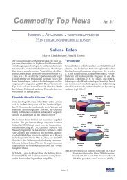
Let us add some remarks for better understanding the zooming process.
This shall be done by discussing a 4-layer case very often occuring in hy-
drogeological prospecting for groundwater. The layer sequence is given in
Fig.18 in logarithmic scale.
Observing the current density j between M and N
at the surface the high resistant second layer will
increase j at the beginning of the zooming process
quite simitar to the simple 2-layer example in
Fig.12-14. The current lines are pushed onto the
surface. Continuing the process, however, the well
conducting third layer will collect the current lines
(pull them downwards) thus causing a decrease of
j at the surface. Finally the aquifer, i.e. the fourth
layer (100Ωm) will push again the current up-
wards.
Fig.18

26
Simulating this zooming by enlarging the distance L between the current
electrodes we shall record a sounding graph ρa( L
2 ) as shown in Fig.19.
Fig.19
The "push and pull"-process can easily be recognized. But looking at the
depth scale on top using the L/2-scale simultaneously we will find no con-
nection between these two scales with respect to the depth of the layer
interfaces and the maximum and mini-
mum of the curve. An optical check will
only result in the resistivity of the first
and of the last layer and the fact that a
4-layer case is concerned. This seems to
be a striking illustration to the final re-
mark in chapter 1.4.: "How deep are you
now?"
The zooming process underlines very
clearly that the logarithmic scale is the
adequate measure for geoelectrical
sounding. Looking at Fig.20 we find at
the right the log. profile of our 4-layer
case (see Fig.18) with interfaces at 2m,
6m and 26m depth. If we multiply these
depths by 10 we get interfaces at 20m,
60m and 260m below surface. This profile

27
is also plotted in log. scale and we see at once that it is congruent to the
first one only shifted along the depth scale. Now "zooming" just means
"shifting along the depth scale" .If we start with the latter case (20, 60,
260m) we will pass during zooming the former case (2, 6, 26m) .The
shape of the sounding graph will not change, i.e. the quality of informa-
tion will always be the same. This has important consequences concerning
the power of solution in sounding graphs. Comparing the profiles in linear
scale on the left side of Fig.20 with the log. profiles on the right side we
find that f.i. the clay-layer (10 Ωm) of 200m thickness in 60 m depth
causes the same minimum in the sounding graph as a 20 m-clay layer in
6m depth.
The authors know that they surpass the aim of this manual by adding
these remarks. But from our opinion the field surveyor should know these
facts to bring him to an advanced level especially in discussions with ge-
ologists: Geologists are thinking "linearely" (bore profiles, well-logging
and even reflection seismics) .In geoelectrics we have to think "logarith-
mically". Here to find a common language is already necessary during
fieldwork; i.e. belongs to the field surveyors duty. If not he will drop back
into a level which can be described by: "He doesn't know what he does!"

28
1.6. Shifting of potential electrodes
In using the Schlumberger arrangement the potential electrodes M and N
are left in their position and only the current electrodes are shifted along
the AB-layout. Of course there will be a limit depending on the sensitivity
of the direct voltage amplifier recording the voltage U. This means that
reaching this limit we are forced to enlarge the spacing MN = a. There
then arise consequences from the theoretical point of view and the
change in surface conditions (lateral effects) around the centre point as
well. In this chapter only the theoretical part shall be discussed. We shall
do this by aid of the 4-layer graph from chapter 1.5. We know that ρa de-
pends on the electrode configuration at the surface. There is a difference
between the apparent resistivity ρa (S) after Schlumberger and ρa (W) after
Wenner. In Fig.21 both curves ρa (S) and ρa (W) are plotted in the same L/2-
diagram.
We observe that the Wenner-curve is a bit "lazy" compared with the
Schlumberger-curve: The ρa (W) curve seems to be pushed to the right;
ascending and decending is not as steep as in ρa (S) ; maximum and mini-
mum of ρa (W) are less extreme than in ρa (S) .This is an important fact to be
taken into account when shifting the potential electrodes.
We will follow this process looking at Fig.22. The initial position of the four
electrodes usually is L/2=1,5m, a/2=0,5m, i.e. we start with Wenner.
Enlarging L/2 and leaving the potential electrodes in their initial position
a/2=0,5m. the recorded ρa-data will smoothly change over from ρa (W) to
ρa (S) . We get the curve branch (1).
At L/2=15 m the U-values recorded by the direct voltage amplifier be-
come very low * . We observe that at least at L/2 = 20 m we will have to
shift the potential electrodes. Branch (1) now is running within the real
Schlumberger curve. Changing the spacing a/2 from 0,5 m to 5 m means
a changing over from Schlumberger to Wenner. The ρa (W) -value at
L/2=15m "drops down" into the Wenner-curve, thus starting branch (2).
* This is only assumed for the present example. In practice we mostly can
run the first branch up to greater L/2-values.

29
The process will be repeated: Enlarging L/2 and keeping a/2=5m fixed we
get a smooth change from ρa (W) into ρa (S) . Assuming we are forced to shift
the potential electrodes again at L/2=60m the ρa (W) -value "jumps" again
but now upward into the dotted Wenner-curve forming the starting point
of branch (3). At L/2=120m we just pass the curve minimum. Due to the
instrument another shifting of the potential electrodes is necessary. In
this position we will record crossing branches (3) and (4).The field opera-
tor should not be irritated. His record is correct because it is a conse-
quence from theory. As this chapter is only dealing with basic laws, prac-
tical advices concerning the shifting of potential electrodes will be given
later on in chapter 2 but making use of the theoretical knowledge just de-
scribed.
As there will be no description of instruments in this manual only one re-
mark should be made concerning unpolarisable potential electrodes. The
main principle is a copperstick put into a solution of copper sulphate con-
tacting the earth via porous porcelain. The type used in our institute is
shown in Fig.23. There are other types, f.i. having a larger bottom or be-
ing porous only in the deeper part. The principle is the same and we must
take care that no crust on the porcelain will interrupt the contact to the
surrounding earth.

30
Fig.21
Fig.22
Fig23

2. Field activities
31
This second chapter should be a guide for field work based on what has
been discussed in the first chapter. It contains advices to the field crew
how to go on to supply the interpreter with optimal data, i.e. the smooth
sounding graphs without errors. From this aim the following - of course
important - points will not be discussed.
1. Instruments: There is a large variety of instruments offered at the
market to carry out direct current resistivity measurements: power supply
by batteries, generators, D.C. amplifiers to feed the current electrodes A
and B, voltmeters as compensators (zero-instruments) or direct voltage
amplifiers to get the voltage between the potential electrodes M and N.
The advices in this manual are independent of the kind of instrument. But
for simplicity a car-borne equipment is taken for demonstration. The ad-
vices can easily be transformed to portable equipments.
2. Safety: As high voltage power (200 V and more) is used safety is a
very severe problem. The assistants at the current electrodes A and B can
be provided by rubber gloves and boots, the steel electrodes can be insu-
lated, an electrical grounding control can be installed at the instrument
etc. Here general advices can of course not be given because the danger
depends on the local situation and the safety is within the responsibility of
the chief surveyor.

32
2.1. How to carry out a field measurement
Now we drive on a measuring car into the field to record a sounding
curve. For this we choose a suitable point in the considered measuring
area, which is the centre point of the measuring lay-out. One shall pay
attention to the potential electrodes. Their site should always be on natu-
rally grown earth.
The direction of the lay-out can be determined by an angle reflector. Then
the measuring car will drive into the right position to the site of the po-
tential electrodes.
In Fig.24 we show a wrong placing of the car. The distance between
measuring car and the potential electrodes is too small, so that already
low leakage currents can more or less influence the potential electrode
voltage. Those leakage currents flow into the earth either via the car or
the cable drums, depending on the resistivity of the first layer.
In Fig.25 the right placing of the measuring car is to be seen. The dis-
tance to the potential electrodes should amount to at least 20m and the
car as well as the cable drums should stand on the “0”-line between the
potential electrodes, running vertically to the potential electrode extent.
This placing of the measuring car should be desirable in every case.
The following processing is schematically demonstrated in Fig.26. When
the car has the right position, the measuring lay-out can be built up. The
cable drums are taken out of the car and set to ground. In order to
enlarge the insulation between the cable drums and the ground, it is rec-
ommended to pose a rubber-mat below each cable drum (Fig.27). On
each drum there is in addition to the electrode cable a 100m long meas-
uring tape (wire of insulating material), on which points are marked for
usual electrode distances according to the table with the geometric factors
K (on page 36). The assistants are walking (or better running) in opposed
directions pulling the measuring tapes. By a stick they fix these measur-
ing tapes at both ends.

Fig25
Fig.26
33
Fig.24

L/2
a/2
1,5 6,28
2 11,8
2,5 18,9
34
Table of K-factors
0,5 1 2 2,5 5 10 20 25 50
3 27,5 12,6
4 49,5 23,6
5 77,7 37,7
6 112 55,0 25,1
(7,5) 176 86,8 41,0 31,4
8 200 990 47,1 36,3
10 313 155 75,4 58,9
12 452 225 110 86,5
(12,5) 490 244 120 94,2
15 706 352 174 137 62,8
20 126 627 311 247 118
25 196 980 488 389 189
30 383 141 704 562 275 126
40 503 251 125 100 495 236
50 785 392 196 157 777 377
60 113 565 282 226 112 550 251
(75) 177 883 441 353 176 868 410 314
80 201 100 502 402 200 990 471 363
100 314 157 785 628 313 155 754 589
120 452 226 113 904 452 225 110 865
(125) 491 245 123 981 490 244 120 942
150 707 353 177 141 706 352 174 137 628
200 628 314 251 126 627 311 247 118
250 982 491 393 196 980 488 389 189
300 141 707 565 283 141 704 562 275
400 126 100 503 251 125 100 495
500 196 157 785 392 196 157 777
600 283 226 113 565 282 226 112
800 503 402 201 100 502 402 200
1000 785 628 314 157 785 628 313

35
The necessary holes for potential electrodes are drilled (f.i. by a cylindri-
cal tube) on those points, which have special signs on the measuring
tape.
One has to pay attention to the holes, which are drilled slightly greater in
comparison to the diameter of the potential electrodes. After the potential
electrodes have been placed into the bore-holes and additionally pressed
closely, in order to maintain the transition resistance between potential
electrodes and ground very low, the cables are connected to the measur-
ing equipment. Finally the electrodes are brought into the initial position
and also connected to the cable drums and measuring equipment respec-
tively.
In order to avoid any influence on the potential electrode voltage the sur-
rounding of the centre point should be kept free ("holy" district). This dis-
trict - to say it again - should be large enough for, even if the cables are
perfectly insulated, "weak" points cannot be avoided where the metal core
is connected to the drums (Fig.27).
Another version of building up the lay-out not using the 100m-measuring
tapes is often applied by field parties where enough labourers are avail-
able, i.e. at least two (better three) of them on the A-direction and the B-
direction as well. By help of a normal tape measure (25m long) small
sticks are put into the ground at the L/2-distances from the centre point
according to the table of K-factors. These sticks carry the L/2 values in
[m] (Fig.28).
No leakage currents then can creep along the measuring tape because
this does not exist. Errors are avoided because each single stick shows
the exact distance.

36
Fig.27 Fig.28
Before we start the measurement we will repeat the preparations looking
at Fig.26 and adding some details:
1 The chief surveyor checks the well at the farm. The depth of the
water table may be of interest for the interpretation of the sound-
ing graph.
2 The "holy" district has to be chosen very carefully. It is recom-
mended to plant 4 potential electrodes at the very beginning:
MN = 1m
and M ' N'
= 10m
and connect them to the equipment by a
double wire (Fig.27). This brings great advantages :
a) during measuring with the smaller distance MN the potential
electrodes M’ and N’ get already "accustomed" to the ground;
b) the overlapping of the Schlumberger branches (see chapter 1.5)
can be done by the operator at the instrument, because calling
the labourers at the current electrodes back and forward again
often leads to errors.
3+4 Assistants marking the lay-out by a tape measure.

37
5+6 Labourers pulling the current cable to the initial position in a wide
bend around the "holy" district. On the drums the cable always
should run from the top (Fig.27).
Now the measurement can start; at each point along the measuring tape
the apparent resistivity ρa is calculated from current I, voltage U and fac-
tor K. In order to determine immediately the right order of the resistivity,
with which the curve starts, significant importance is due to the calcula-
tion of the first value for the apparent resistivity. For L/2=1,5m and
a/2=0,5m the geometrical factor K is 2π=6,28 (exactly 2πa after Wenner,
see chapter 1.3). If now the electrode current I will be adjusted numeri-
cally to the factor K, the potential electrode voltage U is numerically equal
to the apparent resistivity ρa. This results from formula (13) in chapter
1.4
ρ
a
=
U
K
I
In practice normally the following three possibilities at the starting point
result from this:
a.) ρ a[
Ωm] =
U[
mV ]
× 6,
28m
0,
628mA
= U[
mV ] × 10
U[
mV ]
b.) ρ a[
Ωm] = × 6,
28m
= U[
mV ] × 1
6,
280mA
U[
mV ]
c.) ρ a[
Ωm] = × 6,
28m
= U[
mV ] × 0,
1
62,
80mA
Using dry batteries the process I=K cannot be realized. ρa then has to be
calculated on a slide rule or nowadays on a pocket-computer.
The ρa-data are directly plotted on bi-logarithmic transparent paper, and
for a better control written in a minute-book.
Besides the date, site (with height above m.s.l.) and number of the
sounding this minute-book should also contain the measured electrode
current I[mA], the measured potential electrode voltage U[mV] and of
course the apparent resistivity ρa. An additional column seems desirable
for remarks like industrial current, tellurics, weather (rain, sun, wind,
thunderstorm) and perhaps a short description of the field (mash-wire

38
fence, ditch) especially, if the U-data are very low and in the most sensi-
tive ranges of the instrument. For a communication between the operator
and the assistants at the current electrodes surely a loud-voiced
calling is sufficient, and later the motor-horn of the measuring car. For
larger electrode distances a walkie-talkie should be used. Signals can also
be given by coloured flags especially if a portable equipment is used and
L/2 a/2
1,5 0,5
M.B.
[mV]
(164)
300
M.B.
[mA]
(6,28)
ρ
a
=
10 164
2,5 0,5 300 30 248
4 0,5 300 100 282
6 0,5 300 300 270
8 0,5 300 300 255
10 0,5 300 1000 242
12 0,5 300 1000 220
15 0,5 30 100 149
20 0,5 30 300 106
25 0,5 10 300 83,5
25 5,0 100 300 85
30 0,5 10 300 76
30 5,0 100 300 77
40 0,5 10 1000 85
40 5,0 10 1000 82
50 5,0 10 100 90
60 5,0 10 300 97
75 5,0 30 300 108
100 5,0 3 100 121
125 5,0 3 100 126
150 5,0 3 100 143
175 5,0 3 100 157
200 5,0 3 300 164
250 5,0
(0,99)
1
(100)
100 194
U
K
I

39
wireless communication is not permitted.
Knowing how to go on from the initial arrangement L/2=1,5m, a/2=0,5m
we shall proceed step by step looking into the minute book dated
11.Sept.1974 during a survey in the Kalantan-delta around Kota Bharu in
Malaysia near to the coast of the South China Sea. Sounding graph 54 is
concerned. The original data are given on page 40.
As an exercise the reader now should take a sheet of transparent bi-log.
paper and plot the sounding graph after the minute book and the advices
given in the following text.
The initial reading with L/2=1,5m, a/2=0,5m is 164 within the U-range of
300 mV putting the current intensity to 6.28 within the 10 mA-range. This
means from formula (13) an apparent resistivity ρa=164Ωm. We plot this
value on the transparent bi-log paper and write it in order to be sure on
the scale just at this point in the diagram. As long as we use the tech-
nique of putting I=K we only write the range of mV and mA in the minute
book and denote the ρa-value at the right.
Going on with L/2=2,5 m we get an ascending branch up to a maximum
at about L/2=5m. After this a descending branch is recorded until below
100Ωm (L/2=25m) the U-voltage decreases below 10mV. Here we shift
the potential electrodes following the description in chapter 1.6 by a proc-
ess of overlapping the curve branches. In the bi-log. diagram the left
branch should be plotted in small circles (◦) the following branch in
crosses (+). As we shift within the curve minimum we get crossing
branches due to the theory explained in chapter 1.6 (Fig.22).
In this case both pairs of potential electrodes MN and M’N’ were con-
nected to the instrument by using double coil as shown in Fig.26 and 27.
Thus the overlapping could be done by switching from a/2=0,5m to
a/2=5m at the instrument at 3 positions of the current electrodes:
L/2=25, 30, 40m. The advantage of this procedure is obvious: The assis-
tants at the current electrodes A and B will not be aware of the overlap-
ping process. They are marching straight on without being irritated. Call-
ing them back and forward which cannot be avoided when using only sin-
gle coils to the potential electrodes often mistakes will happen as known

40
by experience. The measurement is now continued up to L/2=250m
(K=196).
As under the given circumstances 196mA for the current intensity I could
not be verified, the I=K technique was replaced by taking the reading in
the 100mA range using the full scale. A voltage U=0,99mV was recorded
in the 1mV range. The result was ρa=294Ωm.
Normally the I=K technique is very handy for the operator at the instru-
ment. But running down into lower ranges especially in the U-range, he
should try to use the highest power available for the current end to take
the reading at the right part of the scales on this instrument in order to
get a better accuracy.
In our example L/2 surpasses 100m, i.e. the final point of the measuring
tape or - using the lay-out in Fig. 28 - the last stick. In order to get the
exact distances L/2 at 125m, 150m… coloured marks fixed on the current
cable can be used controlled by a surveyor at the centre point. This is the
most simple way if only one assistant is pulling the current cable. If two
men are working at each current electrode, they can fix the next position
for the electrode by a tape measure (see f.i. (3) + (4) in Fig.26).
In curve 54 under discussion one will miss the readings at L/2= 2, 3 and
5m. To spare time these data are not necessary because the top layer is
not of much interest. We must only know the rough structure of the first
10m in Kota Bharu-area but details in greater depth. To get these details
the curve has to be smooth in its rear branch for an optimal interpreta-
tion. "Jumping" data from say f.i. L/2=100m will bring no information
here and could be thrown off.
If the sounding is finished the assistants at A and B will get a signal by
horn, flag or wireless. They have to disconnect the cable from the elec-
trodes, drop the cable and return with the electrode only to the centre
point. Never take back the end of the cable! The cable has to remain in a
straight line! Otherwise complication may arise in pulling it back to the

41
cable drums. Rewinding it on the drums can be done either by hand or by
an electro-motor driven by the car batteries.
Depending on the surface conditions pulling the current cables very often
is a hard work in case of L/2-distances >300m. This difficulty can be
overcome by adding additional drums brought to A and B by car. Con-
necting them to the ends of the first cables has to be done carefully with
respect to the insulation. This is a really "weak point". We must be sure
that there will be no "leakage" of current. Finally it should be mentioned
that the unpolarisable potential electrodes (see chapter 1.6) are to be
transported - all four of them - within a big plastic bottle filled with a
saturated solution of copper sulphate. Thus the porous porcelain is sur-
rounded by the fluid from in- and outside and cannot dry out. In any case
the electrodes have to be controlled before starting the next measure-
ment that there is enough fluid inside and no crust outside in order to get
a good contact to the ground within the "holy" district.

42
2.2. Possible errors influencing the measurement
It sometimes happens that one or more points of a sounding graph drop
out. The resulting curve cannot be smooth. Some of these possible rea-
sons shall be explained in the following.
2.2.1. Current electrode wrongly grounded: remain standing
When an assistant has not noticed the signal for shifting the electrode and
is remained standing, while the other is moved on, then the distance be-
tween the electrodes A and B is too short in comparison to the configura-
tion factor K. The K used for calculating ρa is therefore too large. This
means, that the apparent resistivity ρa will be too high, i.e. when an assis-
tant is remained standing the point drops out upwards.
2.2.2. Current electrode wrongly grounded: surpassing
When an assistant has missed the following L/2 mark after the signal for
shifting the electrodes and has surpassed it, then the distance between
the electrodes A and B is too large in comparison to the configuration fac-
tor K. The K used for calculating ρa is therefore too small. A too small K,
however, means that a lower apparent resistivity ρa will be recorded. i.e.
when an assistant has surpassed an L/2-mark the point drops out down-
wards.
2.2.3. Wire-mesh-fence (Fig.26/27)
We assume that a wire-mesh-fence in its lower part touches the ground.
With this, a conductive connection to the underground parallel to the
measuring range exists. When the electrode reaches the beginning of the
wire-mesh-fence, there are still no effects at the sounding graph. But
when the electrode passes the wire-mesh-fence and is grounded near to
the fence, it seems that the current flows into the ground at the beginning
of the fence; that means: when the electrode is shifted from the begin-
ning to the end of the fence, it seems that the electrode effectively has
not been moved at all. According to case 2.2.1. the point drops out up-
wards.

43
This result seems to be a paradoxon as we believe that now a nearly per-
fect conductor (wire-mesh-fence) exists and consequently the resistivity
should be reduced. But just the opposite happens, because the current
already flows into the ground nearer to the centre point. This fact shall be
explained once again by observing the current density j between the po-
tential electrodes M and N.
Fig.29
The current electrodes are in position A and B on the surface. In the cen-
tre of the lay-out between the potential electrodes M and N the current
density "below our feet" will be recorded by formula (11) in chapter 1.3.
Without the wire-mesh-fence the current density in position A is greater
than in position A’. But with the wire-mesh-fence it seems after moving
from A to A' that we still have the same current density as in the position
A, i.e. higher than it should be in A'. A higher density effects a higher
voltage between the potential electrodes: the ρa point at A' drops out up-
wards.
On the other hand passing a wooden fence when the connecting wires are
not touching the ground (Fig.29b) the curve will remain smooth.

2.2.4. Crossing a ditch (Fig.26/29)
44
The importance of observing the current density between M and N may be
demonstrated now in the case of a good conducting thin surface layer (ρ1)
underlain by a second layer of higher resistivity (ρ2 > ρ1). This very often
happens in nature, f.i. sand with a thin clayey overburden. We assume
that the current electrode A is crossing a dry ditch cut through the clay as
shown in Fig.29a.
When the electrode A reaches a position just before the ditch, we observe
a high, but a quite normal current density due to the clay cover. But when
the electrode is just behind the ditch (A’) the current lines within the clay
are interrupted. The current has to pass the second layer underneath the
ditch (dotted current lines).
The current density between the potential electrodes will be reduced and
the ρa-point drops out of the sounding graph downwards.
Our conclusion is: when a good conductor (wire-mesh-fence) appears as a
disturbance, the point of a sounding curve drops out upward, when a bad
conductor appears (ditch cutting the first layer) the point drops out
downwards. This is due to the definition of the apparent resistivity. The
apparent resistivity doesn’t deal with the distribution of resistivity in the
underground, but with the current density at the potential electrodes be-
tween M and N.
The current density j is the parameter which is fundamental at all consid-
erations in field works. One has to think in current densities, in order to
get the right conclusions out of the possible disturbances.
2.2.5. Water-pipe parallel to the measuring lay-out (Fig.26/30)
The effect of a water-pipe buried parallel to the measuring lay-out is simi-
lar to that of a wire-mesh-fence, but much more dangerous for interpreta-
tion if both the pipe and L/2-line are running close to each other along a
road or path up to the end of the lay-out. We look at the electrode B in
Fig.26 and 30.

45
Up to the beginning of the water-pipe (dotted line) no effects will influ-
ence the sounding graph. But when the electrode is grounded along the
pipe it seems to remain standing at the beginning of the water-pipe. We
get the upward trend described in 2.2.1. but here as a steady process.
The result is a smooth rear curve branch which may be interpreted as a
high resistant bedrock in greater depth.
If the field surveyor has a bad feeling looking at this ascending branch
which perhaps only appears in just this single sounding and not in graphs
measured at stations in the surrounding area, he has either to try to de-
tect the water-pipe or, if this is not possible because the pipe is buried, to
help himself by a special technique now to be described:
The AB-lay-out normally should be a straight line. A simple trigonometric
calcu-lation, however, shows that the relative error in the ρa-value is less
Fig.30
Fig.30
Fig.30
than even 1% if one
electrode is placed 20%
of the L/2 distance per-
pendicular outside of
the straight lay-out.
With other words:
At L/2=100m the elec-
trode can be shifted
perpendicular to the
AB-line 20m aside hav-
ing an error in the
sounding graph only in
"pencil-thickness" on
the log-log paper.
This surprising fact is
mostly kept as a "se-
cret" not to irritate the
assistants and labour-
ers building up the field
array. If they know that

46
accuracy is not so important they may perhaps be lazy in measuring the
distance from the centre point to the electrode. But this L/2-distance
must be accurate because as we have already seen the K-factor is of
great influence and 1% error in L/2 causes 1% error in the sounding
graph.
In order to check whether the electrode is placed on top of a water-pipe
(or on a buried cable) the electrode may be shifted aside perpendicular to
the normal lay-out. (Doing this one has to take care on a correct right
angle!)
If there is a change in the recorded ρa-value, than the curve is disturbed;
the ascending branch is not real. The same can be done passing a wire-
mesh-fence, and also to by-pass obstacles (houses, small lakes, etc.).
Last not least measuring along a railway or a saltwater channel it can be
check whether there is any influence or not.
Crossing a pipeline which runs somehow perpendicular to the lay-out a
kick will be observed in the graph because just on top of the pipe the
point-electrode will be changed into a line-electrode. Further on the influ-
ence will vanish but difficulties remain for the interpreter because at first
he has to smoothen the graph by hand.
2.2.7. Leakage in the cable
We assume that by shifting the electrodes A and B from L/2=75m to
100m the insulation of one of the electrode cables will be spoiled. This
point of leakage may be invisible for the operator and assistant on the
ground near to one of the potential electrodes. Then the current will run
to ground not only at the grounded electrodes, but additionally at the
point of leakage. This cannot to be observed on the ampere meter, be-
cause the amount of leakage current will be relatively small according to
the high contact resistance at the point of leakage. As this point lies near
to a potential electrode, this additional current flows into the ground, the
current density between M and N increases, and the ρa point consequently
drops out of the sounding graph in upward direction.

47
To get a smooth graph we have to stop the measurement at once and
look for the reason:
1. We check the position of the current electrodes A and B whether
one of the assistants has remained standing accordingto2.2.1.. If
this is alright, then
2. the assistant at A is asked to disconnect his current cable from the
electrode and hold the end of the cable (of course where it is insu-
lated!) in his hand high up in the air so that the real end is free.
Then we supply power and look at the voltmeter putting the U-
range down to high sensitivity. As now current can flow between A
and B the voltmeter has to remain on zero. If there is no reaction
we do the same at B. On one side there must be a reading on the
voltmeter of the instrument.
3. We now check the cable at that side by lifting it up step by step and
will quickly find the spoiled spot. After having insulated the cable
we can continue the measurement.

2.2.8. Insulation and leakage current
48
The insulation presents one of the most important problems in geoelec-
trics. In the following quite real case we may use 200V direct voltage for
the power supply of the electrodes A and B. Between the potential elec-
trodes M and N approximately 2mV are assumed to be measured. In this
example the voltage ratio would be 100 000:1.
One could have the opinion, that a sounding curve is susceptible against
leakage current, when the first layer has a perfect conductivity. That is
however a wrong thinking. The poorer the conductivity of the first layer is
the more susceptible is a curve against leakage current. Another paradox?
We have to study this fact in detail.
From chapter 1 we know that the information about the resistivity distri-
bution in the layered underground is reflected to the earth's surface by
the current density j "below our feet" between the potential electrodes M
and N. As we cannot measure j directly we do it by recording the voltage
U between M and N using the formula from chapter 1.3:
U = j ρ
(11)
a
From this voltage U the apparent resistivity is calculated after formula
(13) given in chapter 1.4:
We now compare two cases
U
a K
I
= ρ (13)
I. high resistivity of the surface layer: ρ1 (I) =10 000 Ωm
II. low resistivity of the surface layer : ρ1 (II) = 10 Ωm
We now assume that our measurements are carried out by using the
same current intensity I and that this current I creates by leakage any-
where outside or inside the instrument an additional current density j’
between M and N. This means that this j’ will keep its value if there is no
change in I.
Taking into account this "disturbing" j’ we have to write formula (11) in
the form
U =
( j + j')
ρ
a
1

and formula (13) will then be
49
U K K
ρa = K = jρ1
+ j'ρ
1
I aI aI
For our two cases I and II this means
K ( I ) K
I. ρ a = j × 10 000 + j'
× 10 000
aI
aI
K ( II ) K
II. ρ a = j × 10 + j'
× 10
aI aI
Comparing the current densities j (I) and j (II) and keeping in mind that
only here the information from the underground with respect to its resis-
tivity distribution is concentrated we see that j (I) is only 1‰ (promille!)
of j (II) because the ratio ρ1 (II) :ρ1 (I) is 1:1000.
From this simple calculation we learn that measuring the same voltage U
between M and N the information from the underground is 1000 times
weaker in the case of a highly resistive surface (case I) than in the case
of a well conducting surface (case II).
Now we look on the second term in the last two formulas containing the
disturbing "quasi-constant" current density j’. Perhaps the reader was a
bit surprised on the form of these last formulas I. and II. because the two
terms on the right side are written in a different way. But in the second
j'
"disturbing" term the quotient is constant in both cases I. and II. The
aI
remaining K × ρ1
is 1000 times larger in case I. than in case II. The result
of comparing both cases will be:
In case I. the first term shows a 1000 times weaker j (I) - that is the underground
information - than in case II. On the other hand the "disturb-
ing" second term with j’ is 1000 times larger in case I. than in case II.
The conclusion will be that in case I. the first term can be neglected as
during continuing the measurement we get into the situation
j (I)

50
Fig.31. They are ascending with an angle of ~63.5° (i.e. arctan(2) from
formula (10) in chapter 1.3), drawn in bi-log. scale.
The result:
On a highly resistive surface a disturbing leakage current will suppress the
underground information (j (I) ) and finally the sounding graph will run into
a 63.5° ascending rear branch. This will happen if j' is positive, i.e. really
added to j (I) .

51
Fig.31

52
If j' is negative, i.e. the disturbing leakage acts against the j (I) than in the
sounding graph we will get in the ρa-values a trend steeply downwards
ending in negative resistivities.
But from experience we know, that already before reaching these final
stages, so-called "clouds" in ρa-values will be a signal, that there is some-
thing wrong.
We have to ask for the origin of these "clouds" .Looking at the last equa-
j'
tion where is assumed to be a constant and the surface resistivity ρ1=
aI
10 000Ωm as well and take into account influences from outside (e.g.
wind and rain) than remembering the very low voltages concerned we
should not be surprised, that a few raindrops may change these parame-
ters. Repeating the measurement will bring then of course different ρa-
values. This is the result of simple physics. If we try to get out of the diffi-
j'
culties caused by the factor the only chance would be increasing the
aI
distance a of the potential electrodes. This can only be done up to a=L/3
(Wenner-arrangement). So-called "Over-Wenner" would bring the poten-
tial electrodes into the neighbourhood of the current electrodes A and B
causing additional difficulties not to be discussed here. Increasing the
spacing a of the potential electrodes will bring at the utmost a factor 10,
increasing the underground influence from 1‰ to 1%.
Comparing this effect with the ratio 1:1000 in ρ1, this will not be a real
help. Increasing I will cause an increasing of the disturbing current den-
sity j' and therefore be no help at all.
The only chance is to look for a surface layer with higher conductivity be-
fore starting a measurement. If there is no chance for finding a centre
point at a surface

53
But we will get those differences if it is raining. Then we have to stop the
measurement at once because wet cables are bad and to dry them will
take a long time. The cable drums should always remain dry, as far as
measurements are bound to a high-resistant surface.
This last chapter should be studied very carefully. A final remark - and
this is an important one - shall be added:
Before opening and checking the instrument always look around outside
the car. Errors occur outside!