Computing Visual Correspondence with Occlusions via Graph Cuts
Computing Visual Correspondence with Occlusions via Graph Cuts
Computing Visual Correspondence with Occlusions via Graph Cuts

You also want an ePaper? Increase the reach of your titles
YUMPU automatically turns print PDFs into web optimized ePapers that Google loves.
The corresponding graph is shown in figure 3. The 3 nodes in the top row<br />
form A 0 and the two nodes in the bottom row form A α .Note,forexample,<br />
that the edge from 〈p, w〉 to 〈p, y〉 has weight ∞, since these two assignments<br />
cannot both be active.<br />
6 Experimental results<br />
Our experimental results involve both stereo and motion. Our optimization<br />
method does not have any parameters except for the exact choice of E. We<br />
selected the labels α in random order, and we started <strong>with</strong> an initial solution<br />
in which no assignments are active. For our data term D we made use of the<br />
method of Birchfield and Tomasi [3] to handle sampling artifacts. The choice<br />
of Va1,a2 was designed to make it more likely that a pair of adjacent pixels<br />
in one image <strong>with</strong> similar intensities would end up <strong>with</strong> similar disparities.<br />
If a1 =〈p, q〉 and a2 =〈r, s〉, thenVa1,a2 was implemented as an empirically<br />
selected decreasing function of max(|I(p) − I(r)|, |I(q) − I(s)|) as follows:<br />
<br />
3λ if max(|I(p) − I(r)|, |I(q) − I(s)|) < 8,<br />
Va1,a2 =<br />
λ otherwise.<br />
(8)<br />
The occlusion penalty was chosen to be 2.5λ for all pixels. Thus, the<br />
energy depends only on one parameter λ. For different images we picked λ<br />
empirically.<br />
We compared the results <strong>with</strong> the expansion algorithm described in [8]<br />
<strong>with</strong> the additional explicit label ’occluded’, since this is the closest related<br />
work. For the data <strong>with</strong> ground truth we obtained some recent results due<br />
to Zitnick and Kanade [25]. We also implemented correlation using the L1<br />
19