Constrained Optimization
Constrained Optimization
Constrained Optimization

You also want an ePaper? Increase the reach of your titles
YUMPU automatically turns print PDFs into web optimized ePapers that Google loves.
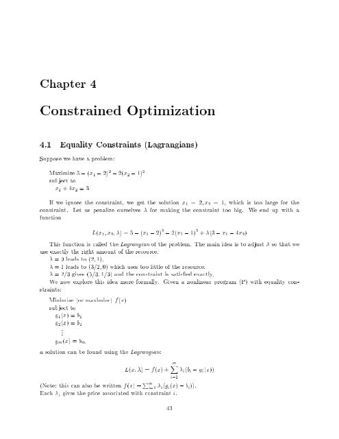
Chapter 4<br />
<strong>Constrained</strong> <strong>Optimization</strong><br />
4.1 Equality Constraints (Lagrangians)<br />
Suppose we have a problem:<br />
Maximize 5 , (x 1 , 2) 2 , 2(x 2 , 1) 2<br />
subject to<br />
x 1 +4x 2 =3<br />
If we ignore the constraint, we get the solution x 1 =2;x 2 = 1, which is too large for the<br />
constraint. Let us penalize ourselves for making the constraint too big. We end up with a<br />
function<br />
L(x 1;x 2; )=5, (x 1 , 2) 2 , 2(x 2 , 1) 2 + (3 , x 1 , 4x 2)<br />
This function is called the Lagrangian of the problem. The main idea is to adjust so that we<br />
use exactly the right amount of the resource.<br />
= 0 leads to (2; 1).<br />
= 1 leads to (3=2; 0) which uses too little of the resource.<br />
=2=3 gives (5=3; 1=3) and the constraint is satis ed exactly.<br />
We now explore this idea more formally. Given a nonlinear program (P) with equality constraints:<br />
Minimize (or maximize) f(x)<br />
subject to<br />
g 1(x) =b 1<br />
g 2(x) =b 2<br />
.<br />
gm(x) =bm<br />
a solution can be found using the Lagrangian:<br />
L(x; )=f(x)+<br />
(Note: this can also be written f(x) , P m i=1 i(gi(x) , bi)).<br />
Each i gives the price associated with constraint i.<br />
43<br />
mX<br />
i=1<br />
i(bi , gi(x))
44 CHAPTER 4. CONSTRAINED OPTIMIZATION<br />
The reason L is of interest is the following:<br />
Assume x =(x 1;x 2;:::;x n) maximizes or minimizes f(x) subject to the<br />
constraints gi(x) =bi, for i =1; 2;:::;m. Then either<br />
(i) the vectors rg 1(x ); rg 2(x );:::;rgm(x ) are linearly dependent,<br />
or<br />
(ii) there exists a vector =( 1 ; 2 ;:::; m) such that rL(x ; )=0.<br />
I.e.<br />
@L<br />
(x ;<br />
@x1 )= @L<br />
(x ;<br />
@x2 )= = @L<br />
(x ;<br />
@xn<br />
)=0<br />
and<br />
@L<br />
(x ;<br />
@ 1<br />
)= = @L<br />
(x ;<br />
@ m<br />
)=0<br />
Of course, Case (i) above cannot occur when there is only one constraint. The following example<br />
shows how it might occur.<br />
Example 4.1.1<br />
Minimize x1 + x2 + x2 3<br />
subject to<br />
x1 =1<br />
x 2<br />
1<br />
+ x2<br />
2 =1:<br />
It is easy to check directly that the minimum is acheived at (x 1;x 2;x 3)=(1; 0; 0). The associated<br />
Lagrangian is<br />
Observe that<br />
and consequently @L<br />
@x2<br />
L(x1;x2;x3; 1; 2)=x1 + x2 + x 2<br />
3 + 1(1 , x1)+ 2(1 , x 2<br />
1 , x2 2):<br />
@L<br />
(1; 0; 0; 1; 2)=1 for all 1; 2;<br />
@x2 does not vanish at the optimal solution. The reason for this is the following.<br />
Let g 1(x 1;x 2;x 3)=x 1 and g 2(x 1;x 2;x 3)=x 2<br />
1 + x 2<br />
2 denote the left hand sides of the constraints.<br />
Then rg 1(1; 0; 0) = (1; 0; 0) and rg 2(1; 0; 0) = (2; 0; 0) are linearly dependent vectors. So Case (i)<br />
occurs here!<br />
Nevertheless, Case (i) will not concern us in this course. When solving optimization problems<br />
with equality constraints, we will only look for solutions x that satisfy Case (ii).<br />
Note that the equation<br />
is nothing more than<br />
@L<br />
(x ; )=0<br />
@ i<br />
bi , gi(x )=0 or gi(x )=bi:<br />
In other words, taking the partials with respect to does nothing more than return the original<br />
constraints.
4.1. EQUALITY CONSTRAINTS (LAGRANGIANS) 45<br />
Once we have found candidate solutions x , it is not always easy to gure out whether they<br />
correspond to a minimum, a maximum or neither. The following situation is one when we can<br />
conclude. If f(x) is concave and all of the gi(x) are linear, then any feasible x with a corresponding<br />
making rL(x ; ) = 0 maximizes f(x) subject to the constraints. Similarly, iff(x) is convex<br />
and each gi(x) is linear, then any x with a making rL(x ; ) = 0 minimizes f(x) subject to<br />
the constraints.<br />
Example 4.1.2<br />
Minimize 2x 2<br />
1<br />
+ x2<br />
2<br />
subject to<br />
x 1 + x 2 =1<br />
L(x1;x2; )=2x2 1 + x2<br />
2 + 1(1 , x1 , x2) @L<br />
(x<br />
@x<br />
1;x2; )=4x1 , 1 =0<br />
1<br />
@L<br />
@x2 (x 1 ;x 2 ; )=2x 2 , 1 =0<br />
@L<br />
@ (x 1;x 2; )=1, x 1 , x 2 =0<br />
Now, the rst two equations imply 2x1 = x2 . Substituting into the nal equation gives the<br />
solution x1 =1=3, x2 =2=3 and =4=3, with function value 2/3.<br />
4<br />
Since f(x1;x2) is convex (its Hessian matrix H(x1;x2)= 0<br />
!<br />
0<br />
is positive de nite) and<br />
2<br />
g(x1;x2)=x1 + x2 constraint.<br />
is a linear function, the above solution minimizes f(x1;x2) subject to the<br />
4.1.1 Geometric Interpretation<br />
There is a geometric interpretation of the conditions an optimal solution must satisfy. Ifwe graph<br />
Example 4.1.2, we get a picture like that in Figure 4.1.<br />
Now, examine the gradients of f and g at the optimum point. They must point in the same<br />
direction, though they may have di erent lengths. This implies:<br />
rf(x )= rg(x )<br />
which, along with the feasibility ofx , is exactly the condition rL(x ; ) = 0 of Case (ii).<br />
4.1.2 Economic Interpretation<br />
The values i have an important economic interpretation: If the right hand side bi of Constraint i<br />
is increased by , then the optimum objective value increases by approximately i .<br />
In particular, consider the problem<br />
Maximize p(x)<br />
subject to<br />
g(x)=b,
46 CHAPTER 4. CONSTRAINED OPTIMIZATION<br />
f(x)=2/3<br />
1<br />
2/3<br />
0<br />
x*<br />
1/3<br />
f= lambda g<br />
g(x)=1<br />
Figure 4.1: Geometric interpretation<br />
where p(x) is a pro t to maximize and b is a limited amount of resource. Then, the optimum<br />
Lagrange multiplier is the marginal value of the resource. Equivalently, ifb were increased by ,<br />
pro t would increase by . This is an important result to remember. It will be used repeatedly<br />
in your Managerial Economics course.<br />
Similarly, if<br />
Minimize c(x)<br />
subject to<br />
d(x) =b,<br />
represents the minimum cost c(x) of meeting some demand b, the optimum Lagrange multiplier<br />
is the marginal cost of meeting the demand.<br />
In Example 4.1.2<br />
Minimize 2x2 1 + x2 2<br />
subject to<br />
x1 + x2 =1,<br />
if wechange the right hand side from 1 to 1:05 (i.e. = 0:05), then the optimum objective function<br />
to roughly<br />
value goes from 2<br />
3<br />
2<br />
3<br />
4 2:2<br />
+ (0:05) =<br />
3 3 :<br />
1
4.1. EQUALITY CONSTRAINTS (LAGRANGIANS) 47<br />
If instead the right hand side became 0:98, our estimate of the optimum objective function value<br />
would be<br />
2<br />
3<br />
4 1:92<br />
+ (,0:02) =<br />
3 3<br />
Example 4.1.3 Suppose we have a re nery that must ship nished goods to some storage tanks.<br />
Suppose further that there are two pipelines, A and B, to do the shipping. The cost of shipping x<br />
units on A is ax 2 ; the cost of shipping y units on B is by 2 , where a>0 and b>0 are given. How<br />
can we ship Q units while minimizing cost? What happens to the cost if Q increases by r%?<br />
Minimize ax 2 + by 2<br />
Subject to<br />
x + y = Q<br />
L(x; y; )=ax 2 + by 2 + (Q , x , y)<br />
@L<br />
(x ;y ;<br />
@x<br />
)=2ax , =0<br />
@L<br />
(x ;y ;<br />
@y<br />
)=2by , =0<br />
@L<br />
(x ;y ; )=Q , x , y =0<br />
@<br />
The rst two constraints give x = b y , which leads to<br />
a<br />
x = bQ<br />
aQ 2abQ<br />
; y = ; =<br />
a + b a + b a + b<br />
and cost of abQ2<br />
a+b . The Hessian matrix H(x 1;x 2)=<br />
2a 0<br />
0 2b<br />
! is positive de nite since a>0 and<br />
b>0. So this solution minimizes cost, given a; b; Q.<br />
If Q increases by r%, then the RHS of the constraint increases by =rQ and the minimum<br />
cost increases by = 2abrQ2<br />
a+b . That is, the minimum cost increases by 2r%.<br />
Example 4.1.4 How should one divide his/her savings between three mutual funds with expected<br />
returns 10%, 10% and 15% repectively, so as to minimize risk while achieving an expected return of<br />
12%. We measure risk as the variance of the return on the investment (you will learn more about<br />
measuring risk in 45-733): when a fraction x of the savings is invested in Fund 1, y in Fund 2 and<br />
z in Fund 3, where x + y + z = 1, the variance of the return has been calculated to be<br />
So your problem is<br />
400x 2 + 800y 2 + 200xy + 1600z 2 + 400yz:<br />
min 400x 2 + 800y 2 + 200xy + 1600z 2 + 400yz<br />
s:t: x + y + 1:5z = 1:2<br />
x + y + z = 1<br />
Using the Lagrangian method, the following optimal solution was obtained<br />
x =0:5 y =0:1 z =0:4 1 = 1800 2 = ,1380
48 CHAPTER 4. CONSTRAINED OPTIMIZATION<br />
where 1 is the Lagrange multiplier associated with the rst constraint and 2 with the second<br />
constraint. The corresponding objective function value (i.e. the variance on the return) is 390.<br />
If an expected return of 12.5% was desired (instead of 12%), what would be (approximately) the<br />
correcponding variance of the return?<br />
Since = 0:05, the variance would increase by<br />
So the answer is 390+90=480.<br />
1 =0:05 1800 = 90:<br />
Exercise 34 Record'm Records needs to produce 100 gold records at one or more of its three<br />
studios. The cost of producing x records at studio 1 is 10x; the cost of producing y records at<br />
studio 2 is 2y 2 ; the cost of producing z records at studio 3 is z 2 +8z.<br />
(a) Formulate the nonlinear program of producing the 100 records at minimum cost.<br />
(b) What is the Lagrangian associated with your formulation in (a)?<br />
(c) Solve this Lagrangian. What is the optimal production plan?<br />
(d) What is the marginal cost of producing one extra gold record?<br />
(e) Union regulations require that exactly 60 hours of work be done at studios 2 and 3 combined.<br />
Each gold record requires 4 hours at studio 2 and 2 hours at studio 3. Formulate the problem of<br />
nding the optimal production plan, give the Lagrangian, and give the set of equations that must<br />
be solved to nd the optimal production plan. It is not necessary to actually solve the equations.<br />
Exercise 35 (a) Solve the problem<br />
max 2x + y<br />
subject to 4x 2 + y 2 =8<br />
(b) Estimate the change in the optimal objective function value when the right hand side increases<br />
by 5%, i.e. the right hand side increases from 8 to 8.4.<br />
Exercise 36<br />
(a) Solve the following constrained optimization problem using the method of Lagrange multipliers.<br />
max ln x +2lny +3lnz<br />
subject to x + y + z =60<br />
(b) Estimate the change in the optimal objective function value if the right hand side of the constraint<br />
increases from 60 to 65.
4.2. EQUALITY AND INEQUALITY CONSTRAINTS 49<br />
4.2 Equality and Inequality Constraints<br />
How dowe handle both equality and inequality constraints in (P)? Let (P) be:<br />
Maximize f(x)<br />
Subject to<br />
g 1(x) =b 1<br />
.<br />
gm(x) =bm<br />
h 1(x) d 1<br />
.<br />
hp(x) dp<br />
If you have a program with constraints, convert it into by multiplying by ,1. Also convert<br />
a minimization to a maximization.<br />
The Lagrangian is<br />
L(x; ; )=f(x)+<br />
The fundamental result is the following:<br />
mX<br />
i=1<br />
i(bi , gi(x)) +<br />
pX<br />
j=1<br />
j(dj , hj(x))<br />
Assume x =(x 1 ;x 2 ;:::;x n) maximizes f(x) subject to the constraints<br />
gi(x) =bi, for i =1; 2;:::;m and hj(x) dj, for j =1; 2;:::;p. Then<br />
either<br />
(i) the vectors rg 1(x );:::;rgm(x ), rh 1(x );:::;rhp(x ) are linearly<br />
dependent, or<br />
(ii) there exists vectors =( 1 ;:::; m) and =( 1 ;:::; p) such<br />
that<br />
rf(x ) ,<br />
mX<br />
i=1<br />
i rgi(x ) ,<br />
pX<br />
j=1<br />
j rhj(x )=0<br />
j (hj(x ) , dj) =0 (Complementarity)<br />
j<br />
0<br />
In this course, we will not concern ourselves with Case (i). We will only look for candidate<br />
solutions x for which we can nd and satisfying the equations in Case (ii) above.<br />
In general, to solve these equations, you begin with complementarity and note that either j<br />
must be zero or hj(x ) , dj = 0. Based on the various possibilities, you come up with one or more<br />
candidate solutions. If there is an optimal solution, then one of your candidates will be it.<br />
The above conditions are called the Kuhn{Tucker (or Karush{Kuhn{Tucker) conditions. Why<br />
do they make sense?<br />
For x optimal, some of the inequalities will be tight and some not. Those not tight can be<br />
ignored (and will have corresponding price j = 0). Those that are tight can be treated as equalities<br />
which leads to the previous Lagrangian stu . So
50 CHAPTER 4. CONSTRAINED OPTIMIZATION<br />
forces either the price j<br />
Example 4.2.1<br />
Maximize x 3 , 3x<br />
Subject to<br />
x 2<br />
The Lagrangian is<br />
So we need<br />
j (hj(x ) , dj) =0 (Complementarity)<br />
to be 0 or the constraint to be tight.<br />
L = x 3 , 3x + (2 , x)<br />
3x 2 , 3 , =0<br />
x 2<br />
(2 , x) =0<br />
Typically, at this point wemust break the analysis into cases depending on the complementarity<br />
conditions.<br />
If = 0 then 3x 2 , 3=0sox =1orx = ,1. Both are feasible. f(1) = ,2, f(,1) = 2.<br />
If x = 2 then = 9 which again is feasible. Since f(2) = 2, we have two solutions: x = ,1 and<br />
x =2.<br />
Example 4.2.2 Minimize (x , 2) 2 +2(y , 1) 2<br />
Subject to<br />
x +4y 3<br />
x y<br />
First we convert to standard form, to get<br />
Maximize ,(x , 2) 2 , 2(y , 1) 2<br />
Subject to<br />
x +4y 3<br />
,x + y 0<br />
L(x; y; 1; 2)=,(x , 2) 2 , 2(y , 1) 2 + 1(3 , x , 4y)+ 2(0 + x , y)<br />
which gives optimality conditions<br />
,2(x , 2) , 1 + 2 =0<br />
,4(y , 1) , 4 1 , 2 =0<br />
0<br />
1(3 , x , 4y) =0
4.2. EQUALITY AND INEQUALITY CONSTRAINTS 51<br />
2(x , y) =0<br />
x +4y 3<br />
,x + y 0<br />
1; 2 0<br />
Since there are two complementarity conditions, there are four cases to check:<br />
1 =0; 2 = 0: gives x =2,y = 1 which is not feasible.<br />
1 =0;x, y = 0: gives x =4=3;y=4=3; 2 = ,4=3 which is not feasible.<br />
2 =0; 3 , x , 4y = 0 gives x =5=3;y=1=3; 1 =2=3 which is O.K.<br />
3 , x , 4y =0;x, y = 0 gives x =3=5;y=3=5; 1 =22=25; 2 = ,48=25 which is not feasible.<br />
Since it is clear that there is an optimal solution, x =5=3;y=1=3 is it!<br />
Economic Interpretation<br />
The economic interpretation is essentially the same as the equality case. If the right hand side<br />
of a constraint ischanged by a small amount , then the optimal objective changes by , where<br />
is the optimal Lagrange multiplier corresponding to that constraint. Note that if the constraint<br />
is not tight then the objective does not change (since then = 0).<br />
Handling Nonnegativity<br />
A special type of constraint is nonnegativity. If you have a constraint xk 0, you can write<br />
this as ,xk 0 and use the above result. This constraint would get a Lagrange multiplier of its<br />
own, and would be treated just like every other constraint.<br />
An alternative is to treat nonnegativity implicitly. If xk must be nonnegative:<br />
1. Change the equality associated with its partial to a less than or equal to zero:<br />
@f(x)<br />
,<br />
@xk<br />
2. Add a new complementarity constraint:<br />
0<br />
@@f(x) ,<br />
@xk<br />
X i<br />
X i<br />
@gi(x)<br />
i ,<br />
@xk<br />
@gi(x)<br />
i ,<br />
@xk<br />
3. Don't forget that xk 0 for x to be feasible.<br />
X j<br />
X j<br />
j<br />
@hj(x)<br />
j<br />
@xk<br />
1<br />
0<br />
@hj(x) A xk =0<br />
@xk
52 CHAPTER 4. CONSTRAINED OPTIMIZATION<br />
Su ciency of conditions<br />
The Karush{Kuhn{Tucker conditions give us candidate optimal solutions x . When are these<br />
conditions su cient for optimality? That is, given x with and satisfying the KKT conditions,<br />
when can we be certain that it is an optimal solution?<br />
The most general condition available is:<br />
1. f(x) is concave, and<br />
2. the feasible region forms a convex region.<br />
While it is straightforward to determine if the objective is concave by computing its Hessian<br />
matrix, it is not so easy to tell if the feasible region is convex. A useful condition is as follows:<br />
The feasible region is convex if all of the gi(x) are linear and all of the hj(x) are convex. If this<br />
condition is satis ed, then any point that satis es the KKT conditions gives a point that maximizes<br />
f(x) subject to the constraints.<br />
Example 4.2.3 Suppose we can buy a chemical for $10 per ounce. There are only 17.25 oz available.<br />
We can transform this chemical into two products: A and B. Transforming to A costs $3 per<br />
oz, while transforming to B costs $5 per oz. If x 1 oz of A are produced, the price wecommand for<br />
Ais$30 , x 1;ifx 2 oz of B are produced, the price we get for B is $50 , x 2. How much chemical<br />
should we buy, and what should we transform it to?<br />
There are many ways to model this. Let's let x 3 be the amount ofchemical we purchase. Here<br />
is one model:<br />
Maximize x1(30 , x1)+x2(50 , 2x2) , 3x1 , 5x2 , 10x3 Subject to<br />
x1 + x2 , x3 0<br />
x3 17:25<br />
The KKT conditions are the above feasibility constraints along with:<br />
30 , 2x 1 , 3 , 1 =0<br />
50 , 4x 2 , 5 , 1 =0<br />
,10 + 1 , 2 =0<br />
1(,x 1 , x 2 + x 3)=0<br />
2(17:25 , x 3)=0<br />
1; 2 0<br />
There are four cases to check:<br />
1 =0; 2 = 0. This gives us ,10 = 0 in the third constraint, so is infeasible.<br />
1 =0;x 3 =17:25. This gives 2 = ,10 so is infeasible.<br />
,x 1 , x 2 + x 3 =0, 2 = 0. This gives 1 =10;x 1 =8:5;x 2 =8:75;x 3 =17:25, which is feasible.<br />
Since the objective is concave and the constraints are linear, this must be an optimal solution. So<br />
there is no point in going through the last case (,x 1 , x 2 + x 3 =0,x 3 =17:25). We are done with<br />
x 1 =8:5;x 2 =8:75; and x 3 =17:25.<br />
What is the value of being able to purchase 1 more unit of chemical?
4.3. EXERCISES 53<br />
This question is equivalent to increasing the right hand side of the constraint x3 17:25 by 1<br />
unit. Since the corresponding lagrangian value is 0, there is no value in increasing the right hand<br />
side.<br />
Review of Optimality Conditions.<br />
The following reviews what we have learned so far:<br />
Single Variable (Unconstrained)<br />
Solve f 0 (x) = 0 to get candidate x .<br />
If f 00 (x ) > 0 then x is a local min.<br />
f 00 (x ) < 0 then x is a local max.<br />
If f(x) is convex then a local min is a global min.<br />
f(x) is concave then a local max is a global max.<br />
Multiple Variable (Unconstrained)<br />
Solve rf(x) = 0 to get candidate x .<br />
If H(x ) is positive de nite then x is a local min.<br />
H(x ) is negative de nite x is a local max.<br />
If f(x) is convex then a local min is a global min.<br />
f(x) is concave then a local max is a global max.<br />
Multiple Variable (Equality constrained) Form Lagrangian L(x; )=f(x)+ P i i(bi , gi(x))<br />
Solve rL(x; ) = 0 to get candidate x (and ).<br />
Best x is optimum if optimum exists.<br />
Multiple Variable (Equality and Inequality constrained)<br />
Put into standard form (maximize and constraints)<br />
Form Lagrangian L(x; )=f(x)+ P i i(bi , gi(x)) + P j j(dj , hj(x))<br />
Solve<br />
rf(x) , P i irgi(x) , P j jrhj(x) =0<br />
gi(x) =bi<br />
hj(x) dj<br />
j(dj , hj(x)) = 0<br />
j<br />
0<br />
to get candidates x (and , ).<br />
Best x is optimum if optimum exists.<br />
Any x is optimum if f(x) concave, gi(x) convex, hj(x) linear.<br />
4.3 Exercises<br />
Exercise 37 Solve the following constrained optimization problem using the method of Lagrange<br />
multipliers.<br />
max 2lnx 1 +3lnx 2 +3lnx 3<br />
s.t. x 1 +2x 2 +2x 3 =10
54 CHAPTER 4. CONSTRAINED OPTIMIZATION<br />
Exercise 38 Find the two points on the ellipse given by x2 1+4x2 2 = 4 that are at minimum distance<br />
of the point (1; 0). Formulate the problem as a minimization problem and solve itbysolving the<br />
Lagrangian equations. [Hint: To minimize the distance d between two points, one can also minimize<br />
d2 . The formula for the distance between points (x1;x2) and (y1;y2)isd2 =(x1 ,y1) 2 +(x2 ,y2) 2 .]<br />
Exercise 39 Solve using Lagrange multipliers.<br />
a) min x2 1 + x2<br />
2 + x2<br />
3 subject to x1 + x2 + x3 = b, where b is given.<br />
b) max p x 1 + p x 2 + p x 3 subject to x 1 + x 2 + x 3 = b, where b is given.<br />
c) min c 1x 2<br />
1 + c 2x 2<br />
2 + c 3x 2<br />
3 subject to x 1 + x 2 + x 3 = b, where c 1 > 0, c 2 > 0, c 3 > 0 and b are given.<br />
d) min x 2<br />
1 + x 2<br />
2 + x 2<br />
3 subject to x 1 + x 2 = b 1 and x 2 + x 3 = b 2, where b 1 and b 2 are given.<br />
Exercise 40 Let a, b and c be given positive scalars. What is the change in the optimum value<br />
of the following constrained optimization problem when the right hand side of the constraint is<br />
increased by 5%, i.e. a is changed to a + 5<br />
100 a.<br />
Give your answer in terms of a, b and c.<br />
max by , x 4<br />
s.t. x 2 + cy = a<br />
Exercise 41 You want toinvest in two mutual funds so as to maximize your expected earnings<br />
while limiting the variance of your earnings to a given gure s2 . The expected yield rates of Mutual<br />
Funds 1 and 2 are r1 and r2 respectively, and the variance of earnings for the portfolio (x1;x2)is 2 2 x1 + x1x2 + 2x2.Thus the problem is<br />
2<br />
max r 1x 1 + r 2x 2<br />
s.t. 2 x 2<br />
1 + x 1x 2 + 2 x 2<br />
2 = s 2<br />
(a) Use the method of Lagrange multipliers to compute the optimal investments x 1 and x 2 in<br />
Mutual Funds 1 and 2 respectively. Your expressions for x 1 and x 2 should not contain the<br />
Lagrange multiplier .<br />
(b) Suppose both mutual funds have the same yield r. Howmuch should you invest in each?<br />
Exercise 42 You want to minimize the surface area of a cone-shaped drinking cup having xed<br />
volume V 0. Solve the problem as a constrained optimization problem. To simplify the algebra,<br />
minimize the square of the area. The area is r p r 2 + h 2 . The problem is,<br />
min<br />
s.t.<br />
2 r 4 + 2 r 2 h 2<br />
1<br />
3 r2 h = V 0:<br />
Solve the problem using Lagrange multipliers.<br />
Hint. You can assume that r 6= 0 in the optimal solution.
4.3. EXERCISES 55<br />
Exercise 43 A company manufactures two types of products: a standard product, say A, and a<br />
more sophisticated product B. If management charges a price of pA for one unit of product A and<br />
a price of pB for one unit of product B, the company can sell qA units of A and qB units of B,<br />
where<br />
qA = 400 , 2pA + pB; qB = 200 + pA , pB:<br />
Manufacturing one unit of product A requires 2 hours of labor and one unit of raw material. For<br />
one unit of B, 3 hours of labor and 2 units of raw material are needed. At present, 1000 hours of<br />
labor and 200 units of raw material are available. Substituting the expressions for qA and qB, the<br />
problem of maximizing the company's total revenue can be formulated as:<br />
max 400pA + 200pB , 2p2 A , p2<br />
B +2pApB<br />
s.t. ,pA , pB ,400<br />
,pB<br />
,600<br />
(a) Use the Khun-Tucker conditions to nd the company's optimal pricing policy.<br />
(b) What is the maximum the company would be willing to pay for<br />
{ another hour of labor,<br />
{ another unit of raw material?
56 CHAPTER 4. CONSTRAINED OPTIMIZATION