Cyclic Voltammetry
Cyclic Voltammetry
Cyclic Voltammetry

You also want an ePaper? Increase the reach of your titles
YUMPU automatically turns print PDFs into web optimized ePapers that Google loves.
<strong>Cyclic</strong> <strong>Voltammetry</strong><br />
Denis Andrienko<br />
January 22, 2008
2<br />
Literature:<br />
1. Allen J. Bard, Larry R. Faulkner “Electrochemical Methods: Fundamentals and Applications”<br />
2. http://www.cheng.cam.ac.uk/research/groups/electrochem/teaching.html
Chapter 1<br />
<strong>Cyclic</strong> <strong>Voltammetry</strong><br />
1.1 Background<br />
<strong>Cyclic</strong> voltammetry is the most widely used technique for acquiring qualitative information about electrochemical<br />
reactions. it offers a rapid location of redox potentials of the electroactive species.<br />
A few concepts has to be introduced before talking about this method.<br />
1.1.1 Electronegativity<br />
Electronegativity is the affinity for electrons. The atoms of the various elements differ in their affinity for<br />
electrons. The term was first proposed by Linus Pauling in 1932 as a development of valence bond theory.<br />
The table for all elements can be looked up on Wikipedia: http://en.wikipedia.org/wiki/Electronegativity.<br />
Some facts to remember:<br />
• Fluorine (F) is the most electronegative element. χF = 3.98.<br />
• The electronegativity of oxygen (O) χO = 3.44 is exploited by life, via shuttling of electrons between<br />
carbon (C, χF = 2.55) and oxygen (O): Moving electrons against the gradient (O to C) - as occurs<br />
in photosynthesis - requires energy (and stores it). Moving electrons down the gradient (C to O) -<br />
as occurs in cellular respiration - releases energy.<br />
• The relative electronegativity of two interacting atoms plays a major part in determining what kind<br />
of chemical bond forms between them.<br />
Examples:<br />
• Sodium (χNa = 0.93) and Chlorine (χCl = 3.16) = Ionic Bond: There is a large difference in<br />
electronegativity, so the chlorine atom takes an electron from the sodium atom converting the<br />
atoms into ions (Na + ) and (Cl − ). These are held together by their opposite electrical charge<br />
forming ionic bonds. Each sodium ion is held by 6 chloride ions while each chloride ion is, in turn,<br />
held by 6 sodium ions. Result: a crystal lattice (not molecules) of common table salt (NaCl).<br />
• Carbon (C) and Oxygen (O) = Covalent Bond. There is only a small difference in electronegativity,<br />
so the two atoms share the electrons. a covalent bond (depicted as C:H or C-H) is formed, where<br />
atoms are held together by the mutual affinity for their shared electrons. An array of atoms held<br />
together by covalent bonds forms a true molecule.<br />
• Hydrogen (H) and Oxygen (O) = Polar Covalent Bond. Moderate difference in electronegativity,<br />
oxygen atom pulls the electron of the hydrogen atom closer to itself. Result: a polar covalent bond.<br />
Oxygen does this with 2 hydrogen atoms to form a molecule of water.<br />
Molecules, like water, with polar covalent bonds are themselves polar; that is, have partial electrical<br />
charges across the molecule; may be attracted to each other (as occurs with water molecules); are good<br />
solvents for polar and/or hydrophilic compounds. May form hydrogen bonds.<br />
3
4 CHAPTER 1. CYCLIC VOLTAMMETRY<br />
1.2 Electrode Reactions<br />
A typical electrode reaction involves the transfer of charge between an electrode and a species in solution.<br />
The electrode reaction usually referred to as electrolysis, typically involves a series of steps:<br />
1. Reactant (O) moves to the interface: this is termed mass transport<br />
2. Electron transfer can then occur via quantum mechanical tunnelling between the electrode and<br />
reactant close to the electrode (typical tunnelling distances are less than 2 nm)<br />
3. The product (R) moves away from the electrode to allow fresh reactant to the surface<br />
The ‘simplest’ example of an electrode reaction is a single electron transfer reaction, e.g. Fe 3+ + e − =<br />
Fe 2+ . Several examples are shown in Fig. 1.1<br />
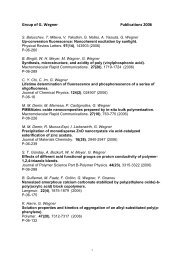
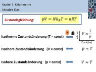
Figure 1.1: Simple electrode reactions: (left) A single electron transfer reaction. Here the reactant<br />
Fe 3+ moves to the interface where it undergoes a one electron reduction to form Fe 2+ . The electron is<br />
supplied via the electrode which is part of a more elaborate electrical circuit. For every Fe 3+ reduced<br />
a single electron must flow. By keeping track of the number of electrons flowing (ie the current) it is<br />
possible to say exactly how many Fe 3+ molecules have been reduced. (middle) Copper deposition at a<br />
Cu electrode. In this case the electrode reaction results in the fomation of a thin film on the orginal<br />
surface. It is possible to build up multiple layers of thin metal films simply by passing current through<br />
appropriate reactant solutions. (right) Electron transfer followed by chemical reaction. In this case an<br />
organic molecule is reduced at the electrode forming the radical anion. This species however is unstable<br />
and undergoes further electrode and chemical reactions.<br />
1.3 Electron Transfer and Energy levels<br />
The key to driving an electrode reaction is the application of a voltage. If we consider the units of volts<br />
V = Joule/Coulomb (1.1)<br />
we can see that a volt is simply the energy required to move charge. Application of a voltage to an<br />
electrode therefore supplies electrical energy. Since electrons possess charge an applied voltage can alter<br />
the ’energy’ of the electrons within a metal electrode. The behaviour of electrons in a metal can be<br />
partly understood by considering the Fermi-level. Metals are comprised of closely packed atoms which<br />
have strong overlap between one another. A piece of metal therefore does not possess individual well<br />
defined electron energy levels that would be found in a single atom of the same material. Instead a<br />
continum of levels are created with the available electrons filling the states from the bottom upwards.<br />
The Fermi-level corresponds to the energy at which the ’top’ electrons sit.
1.4. KINETICS OF ELECTRON TRANSFER 5<br />
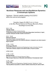
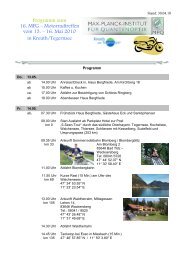
Figure 1.2: Representation of the Fermi-Level in a metal at three different applied voltages (left).<br />
Schematic representation of the reduction of a species (O) in solution (right).<br />
This level is not fixed and can be moved by supplying electrical energy. Electrochemists are therefore<br />
able to alter the energy of the Fermi-level by applying a voltage to an electrode.<br />
Figure 1.2 shows the Fermi-level within a metal along with the orbital energies (HOMO and LUMO)<br />
of a molecule (O) in solution. On the left hand side the Fermi-level has a lower value than the LUMO<br />
of (O). It is therefore thermodynamically unfavourable for an electron to jump from the electrode to<br />
the molecule. However on the right hand side, the Fermi-level is above the LUMO of (O), now it is<br />
thermodynamically favourable for the electron transfer to occur, ie the reduction of O.<br />
Whether the process occurs depends upon the rate (kinetics) of the electron transfer reaction and the<br />
next document describes a model which explains this behavior.<br />
1.4 Kinetics of Electron Transfer<br />
In this section we will develop a quantitative model for the influence of the electrode voltage on the rate<br />
of electron transfer. For simplicity we will consider a single electron transfer reaction between two species<br />
(O) and (R)<br />
O + e − kred<br />
−−→ R (1.2)<br />
R kox<br />
−−→ O + e −<br />
The current flowing in either the reductive or oxidative steps can be predicted using the following<br />
expressions<br />
iO = F AkoxcR<br />
iR = −F AkredcO<br />
For the reduction reaction the current iR is related to the electrode area A, the surface concentration<br />
of the reactant cO, the rate constant for the electron transfer kred and Faraday’s constant F . A similar<br />
expression is valid for the oxidation, now the current is labelled iO, with the surface concentration that of<br />
the species R. Similarly the rate constant for electron transfer corresponds to that of the oxidation process.<br />
Note that by definition the reductive current is negative and the oxidative positive, the difference in sign<br />
simply tells us that current flows in opposite directions across the interface depending upon whether we<br />
are studying an oxidation or reduction. To establish how the rate constants kox and kred are influenced<br />
by the applied voltage we will use transition state theory.<br />
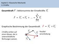
In this theory the reaction is considered to proceed via an energy barrier, as shown in Fig 1.3. The<br />
summit of this barrier is referred to as the transition state. Using this picture the corresponding reaction<br />
rates are given by<br />
<br />
−∆Gred,ox<br />
kred,ox = Z exp<br />
(1.6)<br />
kBT<br />
If we plot a series of the free energy profiles as a function of voltage the free energy of R will be<br />
invariant with voltage, whereas the right handside (O + e) shows a strong dependence.<br />
(1.3)<br />
(1.4)<br />
(1.5)
6 CHAPTER 1. CYCLIC VOLTAMMETRY<br />
Figure 1.3: Transition occurs via a barrier ∆G.<br />
This can be explained in terms of the Fermi level diagrams noted earlier: as the voltage is altered the<br />
Fermi level is raised (or lowered) changing the energy state of the electrons.<br />
However it is not just the thermodynamic aspects of the reaction that can be influenced by this<br />
voltage change as the overall barrier height (ie activation energy) can also be seen to alter as a function<br />
of the applied voltage. We might therefore predict that the rate constants for the forward and reverse<br />
reactions will be altered by the applied voltage. In order to formulate a model we will assume that the<br />
effect of voltage on the free energy change will follow a linear relationship (this is undoubtedly an over<br />
simplification). Using this linear relationship the activation free energies for reduction and oxidation will<br />
vary as a function of the applied voltage as follows (Buttler-Volmer model)<br />
∆Gred = ∆Gred(V = 0) + αF V (1.7)<br />
∆Gox = ∆Gox(V = 0) − (1 − α)F V (1.8)<br />
The parameter α is called the transfer coefficient and typically is found to have a value of 0.5.<br />
Physically it provides an insight into the way the transition state is influenced by the voltage. A value of<br />
one half means that the transition state behaves mid way between the reactants and products response to<br />
applied voltage. The free energy on the right hand side of both of the above equations can be considered<br />
as the chemical component of the activation free energy change, ie it is only dependent upon the chemical<br />
species and not the applied voltage. We can now substitute the activation free energy terms above into<br />
the expressions for the oxidation and reduction rate constants, which gives<br />
kred = Z exp<br />
kox = Z exp<br />
−αF V<br />
exp<br />
kBT kBT<br />
(1 − α)F V<br />
exp<br />
kBT<br />
−∆GV =0<br />
red<br />
−∆GV =0<br />
ox<br />
kBT<br />
(1.9)<br />
(1.10)<br />
These results show us the that rate constants for the electron transfer steps are proportional to the<br />
exponential of the applied voltage. So the rate of electrolysis can be changed simply by varying the applied<br />
voltage. This result provides the fundamental basis of the experimental technique called voltammetry<br />
which we will look at more closely later.<br />
In conclusion we have seen that the rate of electron transfer can be influenced by the applied voltage<br />
and it is found experimentally that this behaviour can be quantified well using the simple model presented<br />
above. However the kinetics of the electron transfer is not the only process which can control the<br />
electrolysis reaction. In many circumstances it is the rate of transport to the electrode which controls<br />
the overall reaction.<br />
1.5 Mass transport<br />
In the electrode kinetics section we have seen that the rate of reaction can be influenced by the cell<br />
potential difference. However, the rate of transport to the surface can also effect or even dominate the<br />
overall reaction rate and in this section we look at the different forms of mass transport that can influence<br />
electrolysis reactions.
1.5. MASS TRANSPORT 7<br />
Figure 1.4: Diffusion of the reactants to the electrode<br />
We have already seen that a typical electrolysis reaction involves the transfer of charge between an<br />
electrode and a species in solution. This whole process due to the interfacial nature of the electron<br />
transfer reactions typically involves a series of steps.<br />
In the section on electrode kinetics we saw how the electrode voltage can effect the rate of the electron<br />
transfer. This is an exponential relationship, so we would predict from the electron transfer model that<br />
as the voltage is increased the reaction rate and therefore the current will increase exponentially. This<br />
would mean that it is possible to pass unlimited quantities of current. Of course in reality this does not<br />
arise and this can be rationalized by considering the expression for the current that we encountered in<br />
the electrode kinetics section<br />
Clearly for a fixed electrode area (A) the reaction can be controlled by two factors. First the rate<br />
constant kred and second the surface concentration of the reactant (Csurf O ). If the rate constant is large,<br />
such that any reactant close to the interface is immediately converted into products then the current will<br />
be controlled by the amount of fresh reactant reaching the interface from the bulk solution above. Thus<br />
movement of reactant in and out of the interface is important in predicting the current flowing. In this<br />
section we look at the various ways in which material can move within solution - so called mass transport.<br />
There are three forms of mass transport which can influence an electrolysis reaction<br />
• Diffusion<br />
• Convection<br />
• Migration<br />
In order to predict the current flowing at any particular time in an electrolysis measurement we will need<br />
to have a quantitative model for each of these processes to complement the model for the electron transfer<br />
step(s).<br />
Diffusion occurs in all solutions and arises from local uneven concentrations of reagents. Entropic<br />
forces act to smooth out these uneven distributions of concentration and are therefore the main driving<br />
force for this process. One example of this can be seen in the animation below. Two materials are held<br />
separately in a single container separated by a barrier. When the barrier is removed the two reagents<br />
can mix and this processes on the microscopic scale is essentially random. For a large enough sample<br />
statistics can be used to predict how far material will move in a certain time - and this is often referred<br />
to as a random walk model. Diffusion is particularly significant in an electrolysis experiment since the<br />
conversion reaction only occurs at the electrode surface. Consequently there will be a lower reactant<br />
concentration at the electrode than in bulk solution. Similarly a higher concentration of product will<br />
exist near the electrode than further out into solution.<br />
The rate of movement of material by diffusion can be predicted mathematically and Fick proposed<br />
two laws to quantify the processes. The first law<br />
∂cO<br />
JO = −DO<br />
∂x<br />
(1.11)<br />
relates the diffusional flux JO (ie the rate of movement of material by diffusion) to the concentration<br />
gradient and the diffusion coefficient DO. The negative sign simply signifies that material moves down a<br />
concentration gradient i. e. from regions of high to low concentration. However, in many measurements<br />
we need to know how the concentration of material varies as a function of time and this can be predicted<br />
from the first law. The result is Fick’s second law<br />
∂cO<br />
∂t<br />
= −∂JO<br />
∂x<br />
(1.12)
8 CHAPTER 1. CYCLIC VOLTAMMETRY<br />
Figure 1.5: Schematic of the setup.<br />
In this case we consider diffusion normal to an electrode surface (x direction). The rate of change of the<br />
concentration cO as a function of time t can be seen to be related to the change in the concentration<br />
gradient. So the steeper the change in concentration the greater the rate of diffusion. In practice diffusion<br />
is often found to be the most significant transport process for many electrolysis reactions.<br />
Fick’s second law is an important relationship since it permits the prediction of the variation of<br />
concentration of different species as a function of time within the electrochemical cell. In order to solve<br />
these expressions analytical or computational models are usually employed.<br />
1.6 <strong>Voltammetry</strong><br />
<strong>Voltammetry</strong> is one of the techniques which electrochemists employ to investigate electrolysis mechanisms.<br />
There are numerous forms of voltammetry<br />
• Potential Step<br />
• Linear sweep<br />
• <strong>Cyclic</strong> <strong>Voltammetry</strong><br />
For each of these cases a voltage or series of voltages are applied to the electrode and the corresponding<br />
current that flows monitored. In this section we will examine potential step voltammetry, the other forms<br />
are described on separate pages<br />
For the moment we will focus on voltammetry in stagnant solution. The figure below shows a schematic<br />
of an electrolysis cell. There is a working electrode which is hooked up to an external electrical circuit.<br />
For our purposes at the moment we will not worry about the remainder of the circuit, obviously there<br />
must be more than one electrode for current to flow. But as we shall see later it is only the so called<br />
working electrode that controls the flow of current flow in the electrochemical measurement. The essential<br />
elements needed for an electolysis measurement are as follows:<br />
• The electrode: This is usually made of an inert metal (such as Gold or Platinum)<br />
• The solvent: This usually has a high dielectric constant (eg water or acetonitrile) to enable the<br />
electrolyte to dissolve and help aid the passage of current.<br />
• A background electrolyte: This is an electrochemically inert salt (eg NaCl or Tetra butylammonium<br />
perchlorate, TBAP) and is usually added in high concentration (0.1 M) to allow the current to pass.<br />
• The reactant: Typically in low concentration 10 −3 M.<br />
1.6.1 Potential Step <strong>Voltammetry</strong><br />
In the potential step measurement the applied voltage is instantaneously jumped from one value V1 to<br />
another V2 The resulting current is then measured as a function time. If we consider the reaction<br />
Fe 3+ (s) + e − kred<br />
−−→ Fe 2+ (s) (1.13)
1.7. LINEAR SWEEP VOLTAMMETRY 9<br />
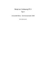
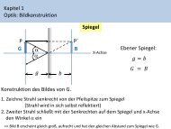
Figure 1.6: Potential step voltammetry: voltage vs time, current versus voltage, and concentration versus<br />
distance from the electrode plotted for several times.<br />
Figure 1.7: Linear increase of the potential vs time.<br />
Usually the voltage range is set such that at V1 the reduction of (Fe 3+ ) is thermodynamically unfavorable.<br />
The second value of voltage (V2) is selected so that any Fe 3+ close to the electrode surface is converted<br />
to product (Fe 2+ ). Under these conditions the current response is in Fig. 1.6.1<br />
The current rises instantaneously after the change in voltage and then begins to drop as a function<br />
of time. This occurs since the instant before the voltage step the surface of the electrode is completely<br />
covered in the reactant and the solution has a constant composition below<br />
Once the step occurs reactant (Fe 3+ is converted to product Fe 2+ and a large current begins to flow.<br />
However now for the reaction to continue we need a supply of fresh reactant to approach the electrode<br />
surface. This happens in stagnant solution via diffusion. As we noted in a previous section the rate of<br />
diffusion is controlled by the concentration gradient. So the supply of fresh Fe 3+ to the surface (and<br />
therefore the current flowing) depends upon the diffusional flux. At short times the diffusional flux of<br />
Fe 3+ is high, as the change in concentration between the bulk value and that at the surface occurs over<br />
a short distance<br />
As the electrolysis continues material can diffuse further from the electrode and therefore the concentration<br />
gradient drops. As the concentration gradient drops (see concentration profiles below) so does<br />
the supply of fresh reactant to the surface and therefore the current also decreases.<br />
Solving the mass transport equation in 1D case we obtain<br />
i = nF Akredc bulk<br />
O<br />
<br />
D<br />
∝ t−1/2<br />
πt<br />
(1.14)<br />
Here the current is related to the bulk reactant concentration. Step voltammetry allows the estimation<br />
of the diffusion coefficients of the species to be obtained.<br />
1.7 Linear Sweep <strong>Voltammetry</strong><br />
In linear sweep voltammetry (LSV) a fixed potential range is employed much like potential step measurements.<br />
However in LSV the voltage is scanned from a lower limit to an upper limit as shown below. The<br />
characteristics of the linear sweep voltammogram depend on a number of factors including:
10 CHAPTER 1. CYCLIC VOLTAMMETRY<br />
Figure 1.8: Linear increase of the potential vs time.<br />
• The rate of the electron transfer reaction(s)<br />
• The chemical reactivity of the electroactive species<br />
• The voltage scan rate<br />
In LSV measurements the current response is plotted as a function of voltage rather than time, unlike<br />
potential step measurements.<br />
The scan begins from the left hand side of the current/voltage plot where no current flows. As the<br />
voltage is swept further to the right (to more reductive values) a current begins to flow and eventually<br />
reaches a peak before dropping. To rationalise this behaviour we need to consider the influence of voltage<br />
on the equilibrium established at the electrode surface. Here the rate of electron transfer is fast in<br />
comparsion to the voltage sweep rate. Therefore at the electrode surface an equilibrum is established<br />
identical to that predicted by thermodynamics. You may recall from equilibrium electrochemistry that<br />
the Nernst equation<br />
The exact form of the voltammogram can be rationalised by considering the voltage and mass transport<br />
effects. As the voltage is initially swept from V1 the equilibrium at the surface begins to alter and the<br />
current begins to flow. The current rises as the voltage is swept further from its initial value as the<br />
equilibrium position is shifted further to the right hand side, thus converting more reactant. The peak<br />
occurs, since at some point the diffusion layer has grown sufficiently above the electrode so that the flux<br />
of reactant to the electrode is not fast enough to satisfy that required by the Nernst equation. In this<br />
situation the curent begins to drop just as it did in the potential step measurements. In fact the drop in<br />
current follows the same behaviour as that predicted by the Cottrell equation.<br />
The above voltammogram was recorded at a single scan rate. If the scan rate is altered the current<br />
response also changes. The figure 1.8 shows a series of linear sweep voltammograms recorded at different<br />
scan rates. Each curve has the same form but it is apparent that the total current increases with increasing<br />
scan rate. This again can be rationalised by considering the size of the diffusion layer and the time taken<br />
to record the scan. Clearly the linear sweep voltammogram will take longer to record as the scan rate is<br />
decreased. Therefore the size of the diffusion layer above the electrode surface will be different depending<br />
upon the voltage scan rate used. In a slow voltage scan the diffusion layer will grow much further from<br />
the electrode in comparison to a fast scan. Consequently the flux to the electrode surface is considerably<br />
smaller at slow scan rates than it is at faster rates. As the current is proportional to the flux towards the<br />
electrode the magnitude of the current will be lower at slow scan rates and higher at high rates. This<br />
highlights an important point when examining LSV (and cyclic voltammograms), although there is no<br />
time axis on the graph the voltage scan rate (and therefore the time taken to record the voltammogram)<br />
do strongly effect the behaviour seen. A final point to note from the figure is the position of the current<br />
maximum, it is clear that the peak occurs at the same voltage and this is a characteristic of electrode<br />
reactions which have rapid electron transfer kinetics. These rapid processes are often referred to as<br />
reversible electron transfer reactions.<br />
This leaves the question as to what would happen if the electron transfer processes were ‘slow’ (relative<br />
to the voltage scan rate). For these cases the reactions are referred to as quasi-reversible or irreversible
1.7. LINEAR SWEEP VOLTAMMETRY 11<br />
Figure 1.9: Change of the rate constant.<br />
Figure 1.10: Voltage as a function of time and current as a function of voltage for CV<br />
electron transfer reactions. The figure below shows a series of voltammograms recorded at a single voltage<br />
sweep rate for different values of the reduction rate constant kred<br />
In this situation the voltage applied will not result in the generation of the concentrations at the<br />
electrode surface predicted by the Nernst equation. This happens because the kinetics of the reaction<br />
are ’slow’ and thus the equilibria are not established rapidly (in comparison to the voltage scan rate).<br />
In this situation the overall form of the voltammogram recorded is similar to that above, but unlike the<br />
reversible reaction now the position of the current maximum shifts depending upon the reduction rate<br />
constant (and also the voltage scan rate). This occurs because the current takes more time to respond<br />
to the the applied voltage than the reversible case.<br />
1.7.1 <strong>Cyclic</strong> <strong>Voltammetry</strong><br />
<strong>Cyclic</strong> voltammetry (CV) is very similar to LSV. In this case the voltage is swept between two values<br />
(see below) at a fixed rate, however now when the voltage reaches V2 the scan is reversed and the voltage<br />
is swept back to V1<br />
A typical cyclic voltammogram recorded for a reversible single electrode transfer reaction is shown in<br />
below. Again the solution contains only a single electrochemical reactant<br />
The forward sweep produces an identical response to that seen for the LSV experiment. When the<br />
scan is reversed we simply move back through the equilibrium positions gradually converting electrolysis<br />
product (Fe 2+ back to reactant (Fe 3+ . The current flow is now from the solution species back to the<br />
electrode and so occurs in the opposite sense to the forward seep but otherwise the behaviour can be<br />
explained in an identical manner. For a reversible electrochemical reaction the CV recorded has certain<br />
well defined characteristics.<br />
1. The voltage separation between the current peaks is<br />
2. The positions of peak voltage do not alter as a function of voltage scan rate
12 CHAPTER 1. CYCLIC VOLTAMMETRY<br />
Figure 1.11: Scan rate and rate constant dependence of the I-V curves.<br />
3. The ratio of the peak currents is equal to one<br />
4. The peak currents are proportional to the square root of the scan rate<br />
The influence of the voltage scan rate on the current for a reversible electron transfer can be seen in<br />
Fig. 1.11 As with LSV the influence of scan rate is explained for a reversible electron transfer reaction<br />
in terms of the diffusion layer thickness. The CV for cases where the electron transfer is not reversible<br />
show considerably different behaviour from their reversible counterparts.<br />
By analysing the variation of peak position as a function of scan rate it is possible to gain an estimate<br />
for the electron transfer rate constants.