Sniffer Adaptive Application Analyzer: Adaptive Mode ... - NetScout

EARLY FIELD TRIAL 

Sniffer ® Adaptive Application Analyzer: 

Adaptive Mode User’s Guide 

733-0204 Rev A 

NetScout ® Systems, Inc. 

Westford, MA 01886 

Telephone: 978.614.4000 

Fax: 978.614.4004 

Web: http://www.netscout.com

accompanies the product at the time of shipment. 

Notice of Restricted Rights: Use, duplication, release, modification, transfer, or disclosure (for purposes 

of this section, "Use") of the Software is restricted by the terms of NetScout Systems, Inc.’s End User 

License Agreement and further restricted in accordance with FAR 52.227-14 for civilian Government 

agency purposes and 252.227-7015 of the Defense Federal Acquisition Regulations Supplement 

("DFARS") for military Government agency purposes, or the similar acquisition regulations of other 

applicable Government organizations, as applicable and amended. The Use of Software and the Product 

is restricted by the terms of NetScout Systems, Inc.’s End User License Agreement, in accordance with 

DFARS Section 227.7202 and FAR Section 12.212. The information in this manual is subject to change 

without notice. 

NetScout, the NetScout logo, Network General, the Network General logo, nGenius, Quantiva, NetVigil, 

InfiniStream, Business Container, and Sniffer are registered trademarks of NetScout Systems, Inc. and/ 

or its affiliates in the United States and/or other countries. The CDM logo, MasterCare, the MasterCare 

logo, Visualizer, and HyperLock are trademarks of NetScout Systems, Inc. All other registered and 

unregistered trademarks herein are the sole property of their respective owners. NetScout Systems, 

Inc. reserves the right, at its sole discretion, to make changes at any time in its technical information, 

specifications, service and support programs. 

All other brand names, company identifiers, trademarks, service trademarks, registered trademarks and 

registered service marks mentioned in this document or the NetScout Systems license agreement are 

properties of their respective owners, and protected as such against unlawful use or distribution. 

This product includes software developed by the Apache Software Foundation 

(http://www.apache.org/). Copyright 1997-2008 The Apache Software Foundation. All rights reserved. 

THE SOFTWARE DEVELOPED BY APACHE SOFTWARE FOUNDATION AND INCLUDED HEREIN IS 

PROVIDED "AS IS" AND ANY EXPRESSED OR IMPLIED WARRANTIES, INCLUDING, BUT NOT LIMITED 

TO, THE IMPLIED WARRANTIES OF MERCHANTABILITY AND FITNESS FOR A PARTICULAR PURPOSE ARE 

DISCLAIMED. IN NO EVENT SHALL THE APACHE SOFTWARE FOUNDATION OR ITS CONTRIBUTORS BE 

LIABLE FOR ANY DIRECT, INDIRECT, INCIDENTAL, SPECIAL, EXEMPLARY, OR CONSEQUENTIAL 

DAMAGES (INCLUDING, BUT NOT LIMITED TO, PROCUREMENT OF SUBSTITUTE GOODS OR SERVICES; 

LOSS OF USE, DATA, OR PROFITS; OR BUSINESS INTERRUPTION) HOWEVER CAUSED AND ON ANY 

THEORY OF LIABILITY, WHETHER IN CONTRACT, STRICT LIABILITY, OR TORT (INCLUDING 

NEGLIGENCE OR OTHERWISE) ARISING IN ANY WAY OUT OF THE USE OF THIS SOFTWARE, EVEN IF 

ADVISED OF THE POSSIBILITY OF SUCH DAMAGE. 

EARLY FIELD TRIAL Use of this product is subject to the NetScout Systems, Inc. End User License Agreement, which


"This product includes software developed by the OpenSSL Project for use in the OpenSSL Toolkit 

(" 

Copyright (c) 1998-2006 The OpenSSL Project. All rights reserved. 

THIS SOFTWARE IS PROVIDED BY THE OpenSSL PROJECT "AS IS" AND ANY EXPRESSED OR IMPLIED 

WARRANTIES, INCLUDING, BUT NOT LIMITED TO, THE IMPLIED WARRANTIES OF MERCHANTABILITY 

AND FITNESS FOR A PARTICULAR PURPOSE ARE DISCLAIMED. IN NO EVENT SHALL THE OpenSSL 

PROJECT OR ITS CONTRIBUTORS BE LIABLE FOR ANY DIRECT, INDIRECT, INCIDENTAL, SPECIAL, 

EXEMPLARY, OR CONSEQUENTIAL DAMAGES (INCLUDING, BUT NOT LIMITED TO, PROCUREMENT OF 

SUBSTITUTE GOODS OR SERVICES; LOSS OF USE, DATA, OR PROFITS; OR BUSINESS INTERRUPTION) 

HOWEVER CAUSED AND ON ANY THEORY OF LIABILITY, WHETHER IN CONTRACT, STRICT LIABILITY, 

OR TORT (INCLUDING NEGLIGENCE OR OTHERWISE) ARISING IN ANY WAY OUT OF THE USE OF THIS 

SOFTWARE, EVEN IF ADVISED OF THE POSSIBILITY OF SUCH DAMAGE. 

"This product includes cryptographic software written by Eric Young (eay@cryptsoft.com) 

" 

"This product includes software written by Tim Hudson (tjh@cryptsoft.com) 

" 

Copyright (c) 1995-1998 Eric Young (eay@cryptsoft.com) All rights 

reserved. 

THIS SOFTWARE IS PROVIDED BY ERIC YOUNG "AS IS" AND ANY EXPRESS OR IMPLIED WARRANTIES, 

INCLUDING, BUT NOT LIMITED TO, THE IMPLIED WARRANTIES OF MERCHANTABILITY AND FITNESS 

FOR A PARTICULAR PURPOSE ARE DISCLAIMED. IN NO EVENT SHALL THE AUTHOR OR CONTRIBUTORS 

BE LIABLE FOR ANY DIRECT, INDIRECT, INCIDENTAL, SPECIAL, EXEMPLARY, OR CONSEQUENTIAL 

DAMAGES (INCLUDING, BUT NOT LIMITED TO, PROCUREMENT OF SUBSTITUTE GOODS OR SERVICES; 

LOSS OF USE, DATA, OR PROFITS; OR BUSINESS INTERRUPTION) HOWEVER CAUSED AND ON ANY 

THEORY OF LIABILITY, WHETHER IN CONTRACT, STRICT LIABILITY, OR TORT (INCLUDING 

NEGLIGENCE OR OTHERWISE) ARISING IN ANY WAY OUT OF THE USE OF THIS SOFTWARE, EVEN IF 

ADVISED OF THE POSSIBILITY OF SUCH DAMAGE. 

Sniffer ® Adaptive Application Analyzer: 

733-0204 Rev A 

Copyright 2010 NetScout Systems, Inc. Printed in the USA. 

All rights reserved.

The best way to contact Customer Support is to submit a Support Request: 

https://my.netscout.com/pages/mcplanding.asp 

Telephone: In the US, call 888-357-7667; outside the US, call 

+011 978-614-4000. Phone support hours are 8 a.m. to 8 p.m. Eastern Standard Time (EST). 

E-mail: support@netscout.com 

When you contact Customer Support, the following information can be helpful in diagnosing and 

solving problems: 

— Type of network platform 

— Software and firmware versions 

— Hardware model number 

— License number and your organization’s name 

— The text of any error messages 

— Supporting screen images, logs, and error files, as appropriate 

— A detailed description of the problem 

Sales 

Call 800-357-7666 for the sales office nearest your location. 

Training 

Course listings and information on nGenius Certification are available at: 

http://www.netscout.com/training 

An extensive library of online course listings, discussion groups, podcasts and best practices is 

available at nGenius Learning 360: 

http://www.netscout.com/training/learning360 

Documentation 

Send comments or questions about nGenius documentation to the following address: 

contact_doc@netscout.com 

User Forum 

To join a customer-driven user group connecting the worldwide community of NetScout users, visit 

the following website: 

http://www.netscoutuserforum.com/ 

RoHS and WEEE 

For compliance information on RoHS and WEEE, visit the NetScout Systems website: 

http://www.netscout.com 

EARLY FIELD TRIAL Customer Support


Contents 

Section 1 

Introduction 

1 Sniffer Adaptive Application Analyzer Overview . . . . . . . . 13 

Overview . . . . . . . . . . . . . . . . . . . . . . . . . . . . . . . . . . . . . . . . . . . . . . 13 

About Sniffer Adaptive Application Analyzer . . . . . . . . . . . . . . . . . . . . . . 13 

About Sniffer Adaptive Intelligence . . . . . . . . . . . . . . . . . . . . . . . . . . . . 16 

Protocols Supported for Sniffer Adaptive Processing . . . . . . . . . . . . . . 18 

What’s Different? . . . . . . . . . . . . . . . . . . . . . . . . . . . . . . . . . . . . . . . . 19 

Key Differences for InfiniStream Console Users . . . . . . . . . . . . . . . . . 19 

Key Differences for Sniffer Portable/Sniffer Global Users . . . . . . . . . . . 22 

Key Terms . . . . . . . . . . . . . . . . . . . . . . . . . . . . . . . . . . . . . . . . . . . . . 23 

2 Quick Start – Five Steps . . . . . . . . . . . . . . . . . . . . . . . . 27 

Overview . . . . . . . . . . . . . . . . . . . . . . . . . . . . . . . . . . . . . . . . . . . . . . 27 

Step 1 – Connecting to the Local Agent . . . . . . . . . . . . . . . . . . . . . . . . . 28 

Step 2 – Selecting Data in the Graph Panel . . . . . . . . . . . . . . . . . . . . . . 31 

Step 3 – Viewing Network Statistics . . . . . . . . . . . . . . . . . . . . . . . . . . . 32 

Step 4 – Capturing Data . . . . . . . . . . . . . . . . . . . . . . . . . . . . . . . . . . . 33 

Step 5 – Mining Packet Data . . . . . . . . . . . . . . . . . . . . . . . . . . . . . . . . 37 

Adaptive Postcapture Analysis . . . . . . . . . . . . . . . . . . . . . . . . . . . . . 39 

Classic Postcapture Analysis . . . . . . . . . . . . . . . . . . . . . . . . . . . . . . 40 

Section 2 

Getting Started 

3 Working with the 

Quick Select Window . . . . . . . . . . . . . . . . . . . . . . . . . . 45 

Overview . . . . . . . . . . . . . . . . . . . . . . . . . . . . . . . . . . . . . . . . . . . . . . 45 

Launching Sniffer Adaptive Application Analyzer . . . . . . . . . . . . . . . . . . . 45 

Introducing the Navigation Panel . . . . . . . . . . . . . . . . . . . . . . . . . . . . . 47 

User’s Guide 5

EARLY FIELD TRIAL Chapter 1 

Opening a Network Interface for Monitoring . . . . . . . . . . . . . . . . . . . . 48 

Other Navigation Panel Tasks . . . . . . . . . . . . . . . . . . . . . . . . . . . . . 49 

Introducing the Graph Panel . . . . . . . . . . . . . . . . . . . . . . . . . . . . . . . . 49 

Using the Time Selector . . . . . . . . . . . . . . . . . . . . . . . . . . . . . . . . . 51 

Viewing “Hover” Statistics . . . . . . . . . . . . . . . . . . . . . . . . . . . . . . . . 53 

Using the Graph Panel Controls . . . . . . . . . . . . . . . . . . . . . . . . . . . . 54 

Introducing the Graph Panel Tabs . . . . . . . . . . . . . . . . . . . . . . . . . . . . . 57 

Global Statistics . . . . . . . . . . . . . . . . . . . . . . . . . . . . . . . . . . . . . . . 57 

Selected Statistics . . . . . . . . . . . . . . . . . . . . . . . . . . . . . . . . . . . . . 59 

Pie Chart . . . . . . . . . . . . . . . . . . . . . . . . . . . . . . . . . . . . . . . . . . . . 61 

Column Chart . . . . . . . . . . . . . . . . . . . . . . . . . . . . . . . . . . . . . . . . 63 

Time Series Chart . . . . . . . . . . . . . . . . . . . . . . . . . . . . . . . . . . . . . 65 

Capture Panel Tab . . . . . . . . . . . . . . . . . . . . . . . . . . . . . . . . . . . . . 66 

Viewing Reports on the Spreadsheet Tab . . . . . . . . . . . . . . . . . . . . . . . . 67 

Using Custom Colors in the Quick Select Window . . . . . . . . . . . . . . . . . . 67 

Sample S2DPalette.ini File . . . . . . . . . . . . . . . . . . . . . . . . . . . . . . . . 69 

4 Using the Statistics Panel . . . . . . . . . . . . . . . . . . . . . . . 71 

Overview . . . . . . . . . . . . . . . . . . . . . . . . . . . . . . . . . . . . . . . . . . . . . . 71 

About the Statistics Panel . . . . . . . . . . . . . . . . . . . . . . . . . . . . . . . . . . 71 

Introducing the Statistics Panel Tabs . . . . . . . . . . . . . . . . . . . . . . . . . . 72 

Spreadsheet Tabs . . . . . . . . . . . . . . . . . . . . . . . . . . . . . . . . . . . . . 72 

Reports Tabs . . . . . . . . . . . . . . . . . . . . . . . . . . . . . . . . . . . . . . . . . 87 

Working with the Statistics Panel . . . . . . . . . . . . . . . . . . . . . . . . . . . . . 93 

Using Statistics Filtering . . . . . . . . . . . . . . . . . . . . . . . . . . . . . . . . . 93 

Refreshing Statistics . . . . . . . . . . . . . . . . . . . . . . . . . . . . . . . . . . . . 97 

Selecting and Deselecting Rows . . . . . . . . . . . . . . . . . . . . . . . . . . . . 97 

Sorting Statistics Panel Tabs . . . . . . . . . . . . . . . . . . . . . . . . . . . . . . 98 

Using the Statistics Panel Tools . . . . . . . . . . . . . . . . . . . . . . . . . . . . 99 

Modifying Statistics Panel Columns and Tabs . . . . . . . . . . . . . . . . . . . . 104 

Adding New Columns . . . . . . . . . . . . . . . . . . . . . . . . . . . . . . . . . . 104 

Adding New Tabs . . . . . . . . . . . . . . . . . . . . . . . . . . . . . . . . . . . . . 106 

Reordering and Deleting Columns and Tabs . . . . . . . . . . . . . . . . . . . 106 

Section 3 

Capturing and Mining Data 

5 Capturing and Mining Data . . . . . . . . . . . . . . . . . . . . . 109 

6 Sniffer Adaptive Application Analyzer


Contents 

Overview . . . . . . . . . . . . . . . . . . . . . . . . . . . . . . . . . . . . . . . . . . . . . 109 

About Capture . . . . . . . . . . . . . . . . . . . . . . . . . . . . . . . . . . . . . . . . . 110 

Configuring and Starting Capture . . . . . . . . . . . . . . . . . . . . . . . . . . . . 111 

Mining Packet Data . . . . . . . . . . . . . . . . . . . . . . . . . . . . . . . . . . . . . . 115 

Using the Mining Summary Dialog . . . . . . . . . . . . . . . . . . . . . . . . . 116 

Using the Progress Panel . . . . . . . . . . . . . . . . . . . . . . . . . . . . . . . . . . 118 

6 Using Filters in the Quick Select Window . . . . . . . . . . . 119 

Overview . . . . . . . . . . . . . . . . . . . . . . . . . . . . . . . . . . . . . . . . . . . . . 119 

About Quick Select Filters . . . . . . . . . . . . . . . . . . . . . . . . . . . . . . . . . 120 

Defining Quick Select Filters . . . . . . . . . . . . . . . . . . . . . . . . . . . . . . . 124 

Working with Auto Filters . . . . . . . . . . . . . . . . . . . . . . . . . . . . . . . 125 

Working with the Filter List Pane (a) . . . . . . . . . . . . . . . . . . . . . . . . 125 

Working with the Filter Editor Pane (c) . . . . . . . . . . . . . . . . . . . . . . 126 

Adding Terms to the Create/Edit Filters Dialog Box . . . . . . . . . . . . . . 129 

Using Pattern Matches with Mining Filters . . . . . . . . . . . . . . . . . . . . 131 

Applying Quick Select Filters . . . . . . . . . . . . . . . . . . . . . . . . . . . . . . . 132 

Applying Mining Filters . . . . . . . . . . . . . . . . . . . . . . . . . . . . . . . . . 133 

Applying Source Filters . . . . . . . . . . . . . . . . . . . . . . . . . . . . . . . . . 134 

Applying Adaptive Display Filters . . . . . . . . . . . . . . . . . . . . . . . . . . 136 

Applying Statistics Filters . . . . . . . . . . . . . . . . . . . . . . . . . . . . . . . 138 

Section 4 

Analyzing Data 

7 Adaptive Session Analysis . . . . . . . . . . . . . . . . . . . . . 141 

Overview . . . . . . . . . . . . . . . . . . . . . . . . . . . . . . . . . . . . . . . . . . . . . 141 

Postcapture Analysis by Capture Mode . . . . . . . . . . . . . . . . . . . . . . . . 141 

Adaptive Mode Postcapture Analysis . . . . . . . . . . . . . . . . . . . . . . . . . . 143 

How Adaptive Processing Works . . . . . . . . . . . . . . . . . . . . . . . . . . . . . 144 

Adaptive Postcapture Analysis Views . . . . . . . . . . . . . . . . . . . . . . . . . . 146 

Adaptive Session View . . . . . . . . . . . . . . . . . . . . . . . . . . . . . . . . . 147 

Adaptive Decode View . . . . . . . . . . . . . . . . . . . . . . . . . . . . . . . . . 153 

Searching Adaptive Views . . . . . . . . . . . . . . . . . . . . . . . . . . . . . . . 158 

Using Filters with Adaptive Postcapture Views . . . . . . . . . . . . . . . . . 159 

Enabling VLAN Data Collection . . . . . . . . . . . . . . . . . . . . . . . . . . . . . . 159 

User’s Guide 7

8 Raw Capture Mode Postcapture Analysis . . . . . . . . . . . 161 


Overview . . . . . . . . . . . . . . . . . . . . . . . . . . . . . . . . . . . . . . . . . . . . . 161 

Introducing the Raw Mode Postcapture Window . . . . . . . . . . . . . . . . . . 162 

Introducing the Packet Decode Tab . . . . . . . . . . . . . . . . . . . . . . . . . . . 165 

Navigating the Decode Tab . . . . . . . . . . . . . . . . . . . . . . . . . . . . . . . . 167 

Selecting Packets in the Decode Tab . . . . . . . . . . . . . . . . . . . . . . . . 170 

Using the Decode Tab Toolbar . . . . . . . . . . . . . . . . . . . . . . . . . . . . 170 

Working with Display Filters . . . . . . . . . . . . . . . . . . . . . . . . . . . . . . . . 172 

Types of Display Filters . . . . . . . . . . . . . . . . . . . . . . . . . . . . . . . . . 173 

Using Automatic Display Filters . . . . . . . . . . . . . . . . . . . . . . . . . . . 174 

Using Quick Filters . . . . . . . . . . . . . . . . . . . . . . . . . . . . . . . . . . . . 178 

Combining Filter Components (“Add to Last Filter”) . . . . . . . . . . . . . 179 

Selecting Filters / Combining Multiple Filters . . . . . . . . . . . . . . . . . . 180 

Using Manual Filters (Display > Define Filter) . . . . . . . . . . . . . . . . . 183 

Using the Manual Display Filter Tabs . . . . . . . . . . . . . . . . . . . . . . . . 185 

Importing and Exporting Filters . . . . . . . . . . . . . . . . . . . . . . . . . . . 190 

Setting Display Setup Options . . . . . . . . . . . . . . . . . . . . . . . . . . . . . . 191 

Display Setup > General Options . . . . . . . . . . . . . . . . . . . . . . . . . . 192 

Display Setup > Summary Display Options . . . . . . . . . . . . . . . . . . . 193 

Display Setup > Packet Selection Options . . . . . . . . . . . . . . . . . . . . 195 

Setting Protocol Aliases for the Postcapture Display . . . . . . . . . . . . . 196 

Searching for Frames in the Decode Display . . . . . . . . . . . . . . . . . . . . . 197 

Printing Decoded Packets . . . . . . . . . . . . . . . . . . . . . . . . . . . . . . . 207 

Using the Matrix Tab . . . . . . . . . . . . . . . . . . . . . . . . . . . . . . . . . . . . . 209 

Using the Host Table Tab . . . . . . . . . . . . . . . . . . . . . . . . . . . . . . . . . . 212 

Using the Protocol Distribution Tab . . . . . . . . . . . . . . . . . . . . . . . . . . . 214 

Using the Statistics Tab . . . . . . . . . . . . . . . . . . . . . . . . . . . . . . . . . . . 216 

Enabling VLAN Data Collection . . . . . . . . . . . . . . . . . . . . . . . . . . . . . . 217 

9 Expert Analysis . . . . . . . . . . . . . . . . . . . . . . . . . . . . . 219 

Overview . . . . . . . . . . . . . . . . . . . . . . . . . . . . . . . . . . . . . . . . . . . . . 219 

Expert Analysis . . . . . . . . . . . . . . . . . . . . . . . . . . . . . . . . . . . . . . . . 219 

Rearranging Expert Panes . . . . . . . . . . . . . . . . . . . . . . . . . . . . . . . 221 

Setting Automatic Expert Display Filters . . . . . . . . . . . . . . . . . . . . . 222 

Displaying Context-Sensitive Explain Messages . . . . . . . . . . . . . . . . 223 

Postcapture Expert/Decode Statistics and CRCs . . . . . . . . . . . . . . . . 224 

Extra Characters in Expert Displays for High Counts? . . . . . . . . . . . . 224 

Saving Expert Objects with Trace Files . . . . . . . . . . . . . . . . . . . . . . 224 



Contents 

Setting Expert Options . . . . . . . . . . . . . . . . . . . . . . . . . . . . . . . . . . . 225 

Objects Tab . . . . . . . . . . . . . . . . . . . . . . . . . . . . . . . . . . . . . . . . . 226 

Alarms . . . . . . . . . . . . . . . . . . . . . . . . . . . . . . . . . . . . . . . . . . . . 229 

Protocols . . . . . . . . . . . . . . . . . . . . . . . . . . . . . . . . . . . . . . . . . . . 231 

Subnet Masks . . . . . . . . . . . . . . . . . . . . . . . . . . . . . . . . . . . . . . . 233 

RIP Options Settings . . . . . . . . . . . . . . . . . . . . . . . . . . . . . . . . . . . 234 

VoIP Options Settings . . . . . . . . . . . . . . . . . . . . . . . . . . . . . . . . . . 236 

Oracle Options . . . . . . . . . . . . . . . . . . . . . . . . . . . . . . . . . . . . . . . 237 

Mobile Options . . . . . . . . . . . . . . . . . . . . . . . . . . . . . . . . . . . . . . . 237 

IP Options . . . . . . . . . . . . . . . . . . . . . . . . . . . . . . . . . . . . . . . . . . 239 

Exporting Expert Data . . . . . . . . . . . . . . . . . . . . . . . . . . . . . . . . . . . . 239 

Section 5 

Additional Information 

10 Setting Quick Select Options . . . . . . . . . . . . . . . . . . . 243 

Overview . . . . . . . . . . . . . . . . . . . . . . . . . . . . . . . . . . . . . . . . . . . . . 243 

Setting General Tab Options . . . . . . . . . . . . . . . . . . . . . . . . . . . . . . . 243 

Setting Connection Tab Options . . . . . . . . . . . . . . . . . . . . . . . . . . . . . 245 

Setting Graph Tab Options . . . . . . . . . . . . . . . . . . . . . . . . . . . . . . . . . 247 

Setting Files Tab Options . . . . . . . . . . . . . . . . . . . . . . . . . . . . . . . . . . 248 

Setting Aliases Tab Options . . . . . . . . . . . . . . . . . . . . . . . . . . . . . . . . 250 

Using Group Aliases Effectively . . . . . . . . . . . . . . . . . . . . . . . . . . . 252 

Setting Options in the Mining Options Tab . . . . . . . . . . . . . . . . . . . . . . 254 

11 Using the Address Book . . . . . . . . . . . . . . . . . . . . . . . 255 

Section 6 

Reporting 

Overview . . . . . . . . . . . . . . . . . . . . . . . . . . . . . . . . . . . . . . . . . . . . . 255 

Introducing the Address Book . . . . . . . . . . . . . . . . . . . . . . . . . . . . . . 255 

Using the Address Book Toolbar . . . . . . . . . . . . . . . . . . . . . . . . . . . 257 

Adding Addresses Manually . . . . . . . . . . . . . . . . . . . . . . . . . . . . . . . . 258 

12 Running Reports . . . . . . . . . . . . . . . . . . . . . . . . . . . . 261 

Overview . . . . . . . . . . . . . . . . . . . . . . . . . . . . . . . . . . . . . . . . . . . . . 261 

User’s Guide 9


Generating Reports . . . . . . . . . . . . . . . . . . . . . . . . . . . . . . . . . . . . . . 261 

Generating Reports from the Spreadsheet Tab . . . . . . . . . . . . . . . . . 261 

Generating Reports From the Reports Tab . . . . . . . . . . . . . . . . . . . . 264 

Modifying the Report Data Window . . . . . . . . . . . . . . . . . . . . . . . . . . . 265 

Printing Reports . . . . . . . . . . . . . . . . . . . . . . . . . . . . . . . . . . . . . . . . 265 

Index . . . . . . . . . . . . . . . . . . . . . . . . . . . . . . . . . . . . 267 



SECTION 1 

Introduction 

Sniffer Adaptive Application Analyzer Overview on 

page 13 

About Sniffer Adaptive Intelligence on page 16 

What’s Different? on page 19 

Key Terms on page 23 

Quick Start – Five Steps on page 27

EARLY FIELD TRIAL


Sniffer Adaptive Application 

Analyzer Overview 

Overview 

1 

This guide describes how to use Sniffer ® Adaptive Application Analyzer 

in Adaptive mode. For information on the Classic mode, refer to the 

Sniffer Adaptive Application Analyzer: Classic Mode User’s Guide. 

This section introduces Sniffer Adaptive Application Analyzer, describes 

the Sniffer Adaptive Intelligence technology, summarizes the major 

features of the software, and orients you to the product as a whole. The 

following topics are covered. 

About Sniffer Adaptive Application Analyzer 

About Sniffer Adaptive Intelligence 

Protocols Supported for Sniffer Adaptive Processing 

What’s Different? 

Key Terms 

About Sniffer Adaptive Application Analyzer 

You can use Sniffer Adaptive Application Analyzer in either Adaptive or 

Classic mode, depending on which entry you select in the Start menu: 

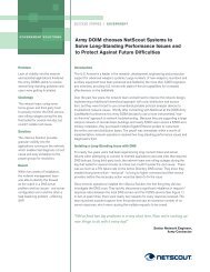
Adaptive Mode – Combines the familiar user interface of the 

InfiniStream ® Console’s Quick Select window with a local Ethernet 

interface and packet buffer (Figure 1-2). In addition, Adaptive 

Intelligence condenses packet information for a range of 

application types while augmenting it with session-awareness, 

providing both the top-down view of a complete session as well as 

its critical packet-level details. 

Classic Mode – Provides all of the functionality traditionally 

associated with NetScout’s Sniffer Portable Professional product, 

including Wi-Fi support, real-time Expert, and full decodes. 

NOTE: Adaptive and Classic modes have separate interfaces. 

Although both interfaces can be open at the same time, 

simultaneously monitoring/capturing data from the Adaptive and 

Classic interfaces is not supported. 

User’s Guide 13


14 Sniffer Adaptive Application Analyzer 

Figure 1-1. Sniffer Adaptive Application Analyzer – One Product, Two 

Modes


Figure 1-2. Adaptive Mode Summary 

Sniffer Adaptive Application Analyzer Overview 

User’s Guide 15

About Sniffer Adaptive Intelligence 



Sniffer Adaptive Application Analyzer introduces new Adaptive Session 

Intelligence technology that streamlines packet-level analysis for 

critical protocols while augmenting it with session-awareness. The 

Adaptive capture mode stores both Adaptive Session Packets (ASPs) for 

bit-level analysis and correlated Adaptive Session Records (ASRs) for 

session analysis: 

Adaptive Session Intelligence extracts and preserves key fields 

from supported packet types, storing condensed Adaptive 

Session Packets (ASPs) rather than raw packets for supported 

protocols. 

ASPs include compressed packet headers through the transport 

layer and an intelligently “derived” payload rather than the actual 

payload. ASPs are much smaller than their raw counterparts and 

can be stored and analyzed much more efficiently. They are also 

correlated with parent Adaptive Session Records for session 

analysis. 

The exact fields preserved in an ASP vary by protocol but include 

compressed MAC/IP headers and key data fields (for example, SQL 

calls embedded in the data portion of an HTTP packet). 

Adaptive Session Records (ASRs) store metadata for flow 

analysis, providing end-to-end transaction metrics, including: 

Source/Destination Identifiers 

Session start/end times 

Latency metrics, success/failure codes, and error messages. 

Application-specific metrics for HTTP, DNS, Media (RTP), Mail 

(SMTP/POP), FTP, and so on. 

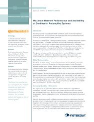
You work with ASRs and ASPs in separate Session and Decode views 

(Figure 1-3). The Adaptive Session and Decode views are very similar to 

the classic Sniffer decode window, allowing you to perform network 

analysis in Summary and Detail panes. Correlation between a session 

and its underlying ASPs let you drill back and forth between the two 

views. You get both the top down view of a complete session and the 

constituent packet level details.



Adaptive Session Packets are 

available for viewing in the 

Adaptive Decode view. 

Standard Summary and Detail 

panes let you browse through 

the events. Here we see one of 

the FTP packets associated 

with the session listed above. 

Use the Open ASR command 

to drill up to the session file 

containing the parent flow. 

Adaptive capture produces 

session records for supported 

protocols. Here we see flow 

statistics for an FTP session. 

Use the Adaptive Packet Drill 

Down command to view the 

underlying packet events. 

Figure 1-3. Sniffer Adaptive Processing – Sessions and Packets 

User’s Guide 17


Using Traditional Packet Capture 


In addition to the new Adaptive capture mode, the Expert analysis and 

raw packet decodes traditionally available in Sniffer products are also 

available in Sniffer Adaptive Application Analyzer. You can change the 

capture mode by clicking the Configure Capture button in the 

Capture toolbar and setting Capture Type to Raw instead of Adaptive 

(the default; Figure 1-4). 

Select the Capture Mode in the 

Configure Capture dialog box. 

Figure 1-4. Setting the Capture Mode 

Protocols Supported for Sniffer Adaptive Processing 

Sniffer Adaptive Application Analyzer supports the following protocols 

for adaptive processing, storing ASPs with derived payloads. For all 

other protocols, you have the choice of capturing full packets, sliced 

packets, or filtering them out entirely. 

HTTP 

FTP 

DNS 

SMTP 

POP3 

RTP 

RTCP 

SIP 

Cisco Skinny


Sample Trace Files 

What’s Different? 


Sniffer Adaptive Application Analyzer is provided with several sets of 

sample trace files in the \Netscout\Sniffer Adaptive 

Application Analyzer\traces folder. Each set contains both a raw packet 

capture (.cap) file and the corresponding Adaptive Traces (.asp/.asr) 

generated by replaying the capture file. 

Each raw packet capture file contains flows using the protocols 

supported for ASI processing listed above. This way, you can compare 

the raw packet file and its corresponding Adaptive Session files to 

understand how the ASI technology works. 

In particular, you can see how Adaptive Intelligence stores key elements 

of supported protocols. For example, the key elements captured for a 

HTTP flow are Host and URL details, while for a RTP flow, the Caller and 

Callee Media Addresses are stored. The sample trace files also 

demonstrate the compression achieved by Adaptive processing – you 

can see at a glance the size differences between the raw and Adaptive 

traces. 

Sniffer Adaptive Application Analyzer’s Adaptive mode combines a 

modified version of the InfiniStream Console user interface with the local 

network interface and packet buffer familiar to users of Sniffer Portable 

Professional and Sniffer Global Application. This section summarizes 

some of the differences users of those products will notice as they work 

with Sniffer Adaptive Application Analyzer in Adaptive mode. 

Key Differences for InfiniStream Console Users 

Users accustomed to working with the InfiniStream Console will notice 

some key differences in Sniffer Adaptive Application Analyzer. Most of 

the differences are due to the differences in how capture/monitoring 

takes place – rather than operating as a unified Console with 

connections to multiple persistent stream-to-disk interfaces on remote 

InfiniStream appliances, Sniffer Adaptive Application Analyzer uses a 

single local Ethernet interface capturing data to a local buffer. 

Key differences between Sniffer Adaptive Application Analyzer and the 

InfiniStream Console summarized below: 

User’s Guide 19

Table 1-1. Key Differences in Sniffer Adaptive Application Analyzer for InfiniStream 

Console Users 

Feature Description 

Local Capture Buffer • The InfiniStream Console connects to remote capture interfaces on 

multiple independent InfiniStream appliances. 

• Sniffer Adaptive Application Analyzer works with a single local 

Ethernet network interface. The Navigation Panel only lists the local 

PC – you can’t add additional remote devices. The local device is 

identified both by its Windows system name and the loopback IP 

address of 127.0.0.1. 

Capture • In the InfiniStream model, capture is “always on,” persistently 

streaming data to vast packet stores spanning multiple disks/array. 

• Sniffer Adaptive Application Analyzer captures data on demand – 

similar to Sniffer Portable/Global, packets are only available after 

you’ve started capture manually. 

Monitoring Statistics • In the InfiniStream model, the InfiniStream appliance tabulates 

RMON statistics persistently. 

• Sniffer Adaptive Application Analyzer only tabulates RMON statistics 

once you’ve opened the local network interface by double-clicking 

its entry in the Navigation Panel at the left of the Quick Select 

window. Once monitoring begins, new statistics are available for 

display in 15 second buckets – you can select a time window from 

the Graph Panel as you normally would. 

Adaptive Analysis Only available in Sniffer Adaptive Application Analyzer. 

Alerts/Alarms Not available in Sniffer Adaptive Application Analyzer. 

InfiniStream 

Administration 

Window 



Not available in Sniffer Adaptive Application Analyzer. 

Sniffer Intelligence Not available in Sniffer Adaptive Application Analyzer. 

Stream Merging Not available in Sniffer Adaptive Application Analyzer.



Table 1-1. Key Differences in Sniffer Adaptive Application Analyzer for InfiniStream 

Console Users 


Sniffer Expert Available when capturing in Raw mode instead of Adaptive mode. Sniffer 

Adaptive Application Analyzer automatically determines which capture 

mode you are using and displays the appropriate analysis interface when 

you click the Mine button to retrieve packet data from a time selection: 

• Adaptive Capture Mode – ASPs are analyzed in the Adaptive 

Session Trace Session and Decode views with drilldowns available 

between the two perspectives. 

• Raw Capture Mode – Packets are analyzed in the traditional 

postcapture Display window with Expert, tri-pane Decode, Matrix, 

Host Table, Protocol Distribution, and Statistics tabs. 

Trace Files • The InfiniStream Console can open Sniffer (.cap) trace files both 

into the Quick Select window and into the postcapture Decode 

window. 

• Sniffer Adaptive Application Analyzer only opens Sniffer trace files 

into the postcapture Decode window using File > Open; you can’t 

add them to the Navigation panel for Quick Select analysis as you 

can with the InfiniStream Console. However, you can also open 

Adaptive trace files (.asr and .asp; refer to Key Terms on page 23 

for a description of these file types). 

User’s Guide 21

Key Differences for Sniffer Portable/Sniffer Global Users 



Users coming to Sniffer Adaptive Application Analyzer’s Adaptive mode 

from Sniffer Portable and Sniffer Global Application will notice some key 

differences. The most obvious difference is the user interface itself – 

rather than using the Sniffer Portable look and feel, Sniffer Adaptive 

Application Analyzer adapts the InfiniStream Console user interface for 

use with a portable network analysis model. 

NOTE: Keep in mind that all traditional Sniffer Portable features are 

still available in Sniffer Adaptive Application Analyzer’s Classic 

mode. 

Key differences between Adaptive and Classic mode are summarized in 

the table below. These same differences also exist between Adaptive 

mode and Sniffer Portable/Sniffer Global Application. 

Table 1-2. Key Differences in Sniffer Adaptive Application Analyzer for Sniffer Portable/ 

Sniffer Global Users 


User Interface Sniffer Adaptive Application Analyzer’s Adaptive mode is based on the 

InfiniStream Console user interface. The Postcapture Display window 

displayed for a Sniffer-format (.cap) trace file is mostly the same 

between the two products, but other features follow the InfiniStream 

Console model. 

Capture • Sniffer Portable/Global provides a Dashboard and Capture Panel 

with live packet counts as well as real-time Expert analysis and 

decodes. 

• Sniffer Adaptive Application Analyzer also provides a Capture Panel, 

though the statistics displayed are not the same. You can observe 

real-time capture in the Graph Panel, make a time selection for realtime 

statistics, and mine any portion of the stream for postanalysis. 

Real-time Expert analysis is not available. 

Monitoring Statistics • In Sniffer Portable/Global, monitoring statistics are collected once 

an adapter is opened and are presented in separate monitor 

applications available from the Monitor menu. 

• Sniffer Adaptive Application Analyzer collects RMON monitoring 

statistics once a network interface is opened and presents them in 

separate tabs in the Statistics panel at the base of the Quick Select 

window instead of in separate applications available from the 

Monitor menu. 

Wi-Fi Analysis Only available in Classic mode (or Sniffer Portable/Sniffer Global 

Application). Sniffer Adaptive Application Analyzer only provides support 

for 100/1000 Mbps Ethernet. 

Adaptive Analysis Only available in Sniffer Adaptive Application Analyzer.


Key Terms 

Table 1-3. Key Terms (1 of 3) 

Terms Definition 

Adaptive Session 

Intelligence 

ASI Protocol 

Interpreters 


Packets (ASPs) 


Records (ASRs) 

Adaptive Capture 

Mode 


The following table defines terms and concepts used in this manual. 

Adaptive Session Intelligence is a Sniffer technology used to streamline 

network analysis by extracting key fields from supported protocols and 

preserving them in a .asp trace file. The .asp trace file is associated with 

a corresponding .asr trace file where correlated session level metadata is 

stored. 

Adaptive Session Intelligence (ASI) Protocol Interpreters condense raw 

packets into Adaptive Session Packets. For supported protocols, ASI 

Protocol Interpreters extract key fields and generate Adaptive Session 

Packets with derived payloads. Other protocols can be captured with the 

raw payload intact or with an optional slice size. 

Condensed “packet events” generated by ASI Protocol Interpreters for 

supported protocols. ASPs consists of compressed headers through Layer 

4 along with key fields extracted from the application payload. 

Adaptive Session Records store session-level metadata for transactions 

observed using supported protocols – for example, an HTTP session, an 

email exchange, and so on. Adaptive Session Records let you view 

combined statistics for entire sessions not available in a single packet. 

Adaptive Session Records are stored in .asr files and are associated with 

corresponding .asp files. You can drill between separate decode views for 

each to see both top-level session statistics and the packet-level details. 

Network capture with Adaptive payload generation enabled (the default). 

You can also use traditional packet capture; refer to Using Traditional 

Packet Capture. 

User’s Guide 23



Network Interface 

(Stream) 

Capture Buffer 

(Store) 



A network interface is the local source of network traffic for Sniffer 

Adaptive Application Analyzer monitoring and capture. Sniffer Adaptive 

Application Analyzer supports a single network interface for monitoring/ 

capture – the Ethernet interface on the local PC. This interface is listed 

under the local laptop’s entry in the Navigation Panel at the left of the 

user interface, like this: 

local laptop/desktop 

network interface 

InfiniStream Console users may be accustomed to referring to the 

network interface as a “stream.” The basic idea is the same – it’s the 

console’s representation of a packet/data gathering interface. However, 

there are several key differences: 

• The Sniffer Adaptive Application Analyzer network interface is on the 

local PC; streams are on remote InfiniStream appliance. 

• Sniffer Adaptive Application Analyzer begins monitoring statistics on 

the network interface when it is opened in the Navigation Panel. 

Packets themselves are only gathered when capture is started 

manually. In contrast, packets/statistics are continuously gathered 

for active streams on InfiniStream appliances. 

• Sniffer Adaptive Application Analyzer only has a single network 

interface – the Ethernet interface on the local laptop (identified in 

the list using the loopback IP address of 127.0.0.1). In contrast, the 

InfiniStream Console works with multiple remote appliances, each 

with multiple network streams. 

Sniffer Adaptive Application Analyzer stores captured packet and 

metadata in an in-memory capture buffer on the local PC. Recorded data 

stored in the capture buffer can be saved to trace files for permanent 

storage. 

InfiniStream Console users may be accustomed to referring to the 

capture buffer as “the store.” The basic idea is the same – a place to 

keep capture packets/metadata. However, there are several key 

differences between the Sniffer Adaptive Application Analyzer capture 

buffer and the store on an InfiniStream appliance: 

• Capture buffer is on the local PC; the store is on a remote 

InfiniStream appliance. 

• Capture buffer is designed for short-term recording and is filled on 

demand when capture starts; the store is a persistent stream-todisk 

operation designed for long-term forensic storage and analysis. 

• Capture buffer is relatively small (up to 1GB) and can be saved to 

trace files; the store is massive, typically spanning multiple disks/ 

arrays. 

• Capture buffer is dynamic and is removed when the application 

shuts down; the store is persistent.





Statistical Data Statistical Data refers to the RMON network statistics tabulated and 

presented in the Statistics panel at the base of the Quick Select window. 

Statistical Data includes traditional packet/byte counts broken out by 

MAC address, IP address, application port, conversation, and so on. 

Sniffer Adaptive Application Analyzer begins monitoring statistical data 

when you double-click the local network interface in the Navigation Panel 

– the Graph Panel will begin to update and display traffic volume over 

time. However, Sniffer Adaptive Application Analyzer does not record 

packets until you manually start capture. 

You can use the color-coded Availability Meter at the base of the Graph 

Panel to determine where both packets and statistics are available and 

where only statistics are available. Refer to Availability Meter on page 56 

for details. 

Time Selection After Sniffer Adaptive Application Analyzer begins capturing packets, you 

can select a segment of the available packets in the Graph Panel for 

analysis. That segment – a portion of the available packets with a 

beginning and end time – is called a time selection. You must make a 

time selection before you can analyze or mine the stream’s data. 

Data Mining Data mining, or mining, refers to your ability to retrieve some of the 

packets in the capture buffer using your own custom search criteria. 

Mining allows you to locate specific sets of packets and conversations 

within the available data. 

Mining Filter A mining filter is a user-configured set of packet criteria and Boolean 

logic you can use to sift through data in the capture buffer. 

Source Filter A source filter is a user-configured set of packet criteria and Boolean 

logic Sniffer Adaptive Application Analyzer uses to filter unwanted 

packets before they are used for RMON monitoring or recorded to the 

capture buffer. Use these with care, since those packets you filter out are 

irretrievable. 

User’s Guide 25




Quick Start – Five Steps 

Overview 

This section describes how to get started using Sniffer Adaptive 

Application Analyzer: 

Step 1 – Connecting to the Local Agent on page 28 

Step 2 – Selecting Data in the Graph Panel on page 31 

Step 3 – Viewing Network Statistics on page 32 

Step 4 – Capturing Data on page 33 

Step 5 – Mining Packet Data on page 37 

NOTE: Sniffer Adaptive Application Analyzer should be installed on 

a machine that meets or exceeds the system requirements before 

using these steps. 

Refer to the Sniffer Adaptive Application Analyzer Installation Guide for 

system requirements, as well as details on which NetScout 

applications can be installed on the same machine as Sniffer 

Adaptive Application Analyzer. 

2 

User’s Guide 27

Step 1 – Connecting to the Local Agent 



Once you’ve installed Sniffer Adaptive Application Analyzer, you’re ready 

to start the application, open the local network interface in the 

Navigation panel, and view its traffic in the Graph and Statistics panels. 

1 On the Console machine, go to Start > (All) Programs > 

NetScout > Sniffer Adaptive Application Analyzer > and 

select the Sniffer (Adaptive Mode) entry to launch Sniffer 

Adaptive Application Analyzer. The Quick Select window appears 

displaying the Navigation, Graph, and Statistics panels (Figure 

2-1): 

Navigation 

Panel 

The Navigation panel lists the network interfaces available 

for monitoring and capture on the local PC. See Using the 

Navigation Panel on page 41. 

The Graph panel displays a graphical representations of the 

local network interface’s traffic. The Graph controls let you 

browse the available data statistics and select a specific time 

period for analysis. See Working with the Quick Select Window 

on page 45. 

The Statistics panel displays the data statistics for a variety 

of traffic elements within the time selection in the Graph 

panel. See Using the Statistics Panel on page 71. 

Graph Panel 

Statistics Panel 

Figure 2-1. Initial View of the Quick Select Window


Double-click the local PC’s entry in 

the Navigation Panel. The local PC is 

indicated with both the MS-Windows 

system name and the loopback IP 


The local PC’s entry cascades open to 

show the network interface available 

for monitoring. Double-click the 

interface to start monitoring. 

Monitoring begins. Data is available 

for display in the Graph and Statistics 

panels after the completion of the 

first 15-second collection bucket. 


2 When you first start Sniffer Adaptive Application Analyzerin 

Adaptive mode, the Graph and Statistics panels are both empty. 

Open a network interface for monitoring to start statistics 

collection: 





selected for monitoring 

NOTE: Note that the console assigns a color and letter to the 

interface. The letter indicates the order in which interfaces 

were opened (for example, the first interface is assigned the 

letter A). These designations are used for stream merging and 

are cosmetic in this release – only a single network interface is 

supported. 

3 Once the first bucket of statistics is collected, click either the Next 

Time Selection or Current Time button above the Graph 

Panel to populate it with bars illustrating the progress of statistics 

collection (Figure 2-2). 

User’s Guide 29



Figure 2-2. Graph Panel with Statistics Collection in Progress



Step 2 – Selecting Data in the Graph Panel 

Once you’ve opened a network interface for monitoring and the Graph 

Panel is illustrating the progress of statistics collection, you can make a 

time selection to view statistics in detail: 

1 In the Graph panel, drag the Time Selector (a) handles to the 

area in the stream you would like to analyze. See Using the Time 

Selector on page 51 for more information. 

Use the Graph panel controls (b) to travel in time within the stream 

and climb/descend the data window axis. See Using the Graph 

Panel Controls on page 54 for more information. 

Figure 2-3. Graph Panel 

b 

a 

a 

User’s Guide 31

Step 3 – Viewing Network Statistics 



1 The Statistics panel displays traffic statistics for the time selection 

made in the Graph panel. You can check IP addresses and/or other 

entries in the Statistics panel tabs to display only selected statistics 

in the Graph panel. See Using the Statistics Panel Tools on page 99 

for more information. 

Figure 2-4. Statistics Panel 

2 Using the Statistics panel controls, filter and sort the data until you 

have isolated the packets you would like to analyze. See the 

following sections for details on Statistics panel tasks: 

Working with the Statistics Panel on page 93 

Using Statistics Filtering on page 93 

Selecting a Statistics Filter on page 94 

Working with the Top N Feature on page 95 

Selecting and Deselecting Rows on page 97 

Using the Statistics Panel Tools on page 99 

Showing/Clearing Highlights on page 100 

Collapsing and Expanding Column Data on page 100 

Using the Mining Summary Dialog on page 116


Step 4 – Capturing Data 


RMON statistics are valuable for understanding the network entities and 

traffic volumes on your network. Network troubleshooting, however, 

usually requires packet analysis. Use the following procedure to set the 

capture mode and start capture. 

1 Click the Configure Capture button and select the capture mode 

(Figure 2-5) – either Adaptive Capture or Raw Capture. 

Figure 2-5. Configuring the Capture Mode 

The table below summarizes the differences between the two 

modes as well as the postcapture analysis views available for each: 

User’s Guide 33

Capture 


Adaptive 

Capture 

(Default) 

Raw 

Capture 


Summary Postcapture Analysis 

In Adaptive Capture mode, Sniffer Adaptive 

Application Analyzer extracts key fields 

from supported protocols and generates 

Adaptive Session Packets (ASPs) with 

derived payloads and compressed packet 

headers through the transport (TCP/UDP) 

layer. Hexadecimal bytes are not displayed 

for ASPs. 

In addition, Sniffer Adaptive Application 

Analyzer stores metadata correlating ASPs 

with parent sessions to provide a flowaware 

view of network data. You can drill 

between the session view and the decode 

view during postcapture analysis to get 

both the top-down and bottom-up 

perspective. 

In Raw Capture mode, Sniffer Adaptive 

Application Analyzer records packets as 

seen on the wire, including payloads (an 

optional packet slice setting can be used). 

In addition session statistics are not 

available. Instead, traditional tri-paned 

packet decodes, Expert analysis, and postanalysis 

tabs are available. 


Separate, correlated views provide 

session and packet statistics: 

• Adaptive Session View provides 

access to adaptive session records 

(ASRs). 

• Adaptive Decode View provides 

line by line interpretation of 

adaptive session packets (ASPs). 

Refer to About Sniffer Adaptive 

Intelligence on page 16 for a summary 

of these two views. 

• Tri-pane packet decodes 

• Expert analyzer 

• Post-analysis tabs (Host Table, 

Matrix, Protocol Distribution, 

Statistics) 

2 Specify the Capture Buffer size (200 MB - 1 GB).


Capture 



Capture 

(Default) 

Raw 

Capture 


3 Set the Packet Slice Size option for your capture mode: 

Available Packet 

Slice Option 

Adaptive Packet 

Slice Size 

Raw Packet Slice 

Size 

Description 

When Adaptive capture is enabled, Sniffer Adaptive 

Application Analyzer generates Adaptive Session Packets for 

all protocols with an ASI Protocol Interpreter. You use the 

Adaptive Packet Slice Size option to specify how much of 

each packet without an ASI protocol interpreter Sniffer 

Adaptive Application Analyzer should capture. 

There are two classes of packets without an ASI Protocol 

Interpreter: 

• Standard IPv4 Protocols on Well-Known TCP/UDP 

Ports 

Sniffer Adaptive Application Analyzer still records generic 

session metadata for these protocols, either listing them 

using hardcoded aliases or identifying them as GENERIC 

(refer to Session View for GENERIC Protocols on page 150 

for details. 

• Others (Non-IPv4) 

Sniffer Adaptive Application Analyzer does not record any 

session metadata for these packets. 

Refer to Protocols Supported for Sniffer Adaptive Processing 

on page 18 for a list of protocols with ASI protocol 

interpreters. 

When Raw capture is enabled, you use the Raw Packet 

Slice Size option to specify how much of each packet to 

capture. 

4 Click OK in the Configure Capture dialog box when you have 

finished configuring capture. 

5 Start capture with either the Start Capture button in the toolbar 

or the Quick Select > Start Capture menu item. 

6 Once you start capturing packets, the Availability Meter at the base 

of the Graph panel changes from Yellow to Green (Figure 2-6), 

indicating that both packets and monitoring statistics are available. 

You can view statistics in the Statistics panel, as well as mine this 

portion of the stream for packets. Refer to Availability Meter on 

page 56 for details. 

User’s Guide 35



Figure 2-6. Availability Meter after Capture Starts 

Availability Meter changes from yellow 

to green when capture starts, 

indicating packets and statistics are 

available for the time selection.


Step 5 – Mining Packet Data 

Capture 



Capture 

(Default) 


You mine available packet data (adaptive or raw) for postcapture 

analysis by making a time selection in the Graph Panel and clicking the 

Mine button at the base of the Quick Select window: 

1 Use the Availability Meter to identify and select a segment of packet 

data in the the Graph Panel. Packet data is indicated by green in 

the Availability Meter. 

2 Create an optional Auto Mining Filter by selecting entities in the 

Statistics Panel. For example, you could create an Auto Mining 

Filter by selecting individual IP addresses in the IP Address tab. 

3 Click Mine. 

4 If you created an optional Auto Mining Filter, click Edit Filter in the 

Summary dialog box to use it for mining. 

5 Refine your mining request as desired and click OK to begin packet 

mining. 

Postcapture Analysis by Capture Mode – Adaptive or Packets 

Sniffer Adaptive Application Analyzer mines the selected time window 

and automatically launches the postcapture analysis views 

corresponding to your capture mode, as summarized in the table and 

Figure 2-7: 

Postcapture Analysis Views Refer to: 

Separate, correlated views provide session and packet 

statistics: 

• Adaptive Session View 

• Adaptive Decode View (two-pane) 

Raw Capture • Tri-pane packet decodes 


• Post-analysis tabs (Host Table, Matrix, Protocol 

Distribution, Statistics) 


Postcapture 

Analysis on page 39 

Classic Postcapture 

Analysis on page 40 

User’s Guide 37



Figure 2-7. Postcapture Analysis by Capture Mode (Adaptive or Raw)


Adaptive Postcapture Analysis 


When capturing in Adaptive mode, clicking Mine displays the selected 

packet data in the Adaptive Decode and Adaptive Session views (Figure 

2-8). 

Adaptive Session Packets are 

available for viewing in the 

Adaptive Decode view. 

Standard Summary and Detail 

panes let you browse through 

the events. Here we see one of 

the FTP packets associated 

with the session listed above. 





session records for supported 

protocols. Here we see flow 

statistics for an FTP session. 




Figure 2-8. Adaptive Session Intelligence Postcapture Analysis 

User’s Guide 39

Classic Postcapture Analysis 



When capturing in Classic mode, clicking Mine displays the selected 

packets in the postcapture display window (Figure 2-9): 

The postcapture display window features two main tabs – Expert and 

Decode – as well as a variety of others providing different views of the 

data. Available tabs are summarized in the table below: 

a b 

Postcapture display tabs. The Decode 

tab always appears. The other tabs 

appear by default, but can be disabled. 

c d e 

Figure 2-9. Classic Postcapture Analysis


Table 2-1. Postcapture Display Tabs 

Tab Description 


Expert Displays the results of proprietary Expert analysis, showing network objects, 

symptoms, and diagnoses by network layer: 

•The Expert Overview (a) pane shows the network analysis layers (similar in 

concept to the ISO layers) and the Expert overview statistics (objects, 

symptoms, or diagnoses) for each layer. 

•The Expert Summary (b) pane shows key summary information for the layer 

and statistics selected in the Expert Overview panel. 

•The Protocol Statistics (c) pane displays the amount of traffic (in frames 

and bytes) for each protocol encountered for the layer you selected in the 

Expert Overview panel. 

•The Detail Tree (d) pane shows a hierarchical listing of all layers below those 

selected in the Expert Overview and Expert Summary panels. 

•The Expert Details (e) pane is a collection of information tables for the data 

selected in the Summary pane. 

See Expert Analysis on page 219. 

Decode Provides classic, line-by-line protocol decodes in a tri-pane window. Sophisticated 

automatic filtering features let you select a packet in the Summary pane and 

automatically filter on different components of the packet (source/destination 

addresses, ports, and so on). 

See Introducing the Packet Decode Tab on page 165. 

Matrix Provides statistics on conversations taking place on the network. 

See Using the Matrix Tab on page 209 

Host Table Provides statistics broken out for each host detected on the network. Different tabs 

let you focus on IP hosts, MAC hosts, and so on. 

See Using the Host Table Tab on page 212. 

Protocol 

Distribution 

Provides statistics broken out by protocol family. You can focus on MAC, IP, or IPX 

layer protocols. 

See Using the Protocol Distribution Tab on page 214. 

Statistics Provides a variety of global statistics, including capture start/stop times, average 

speeds, and packet counts for a variety of basic categories. 

See Using the Statistics Tab on page 216. 

Filtered 

Tabs 

By default, display filters return the filtered frames in a new tab at the bottom of 

the postcapture display window. If you prefer, you can enable the Select 

matching option. When this option is enabled, frames matching the filter appear 

“marked” in the leftmost column of the active Decode tab – their checkboxes are 

checked. 

See Working with Display Filters on page 172 for more information on how to use 

display filters in the Decode tab. 

User’s Guide 41



6 You can optionally apply a Display Filter to isolate specific packets, 

including Automatic and Quick display filters. Display filters are 

helpful when working with large volumes of data. Use Display 

Filters to reduce large data sets when you are looking for 

something in particular. See Working with Display Filters on page 

172. 

7 Click the Quick Select icon to jump back to the Quick Select 

window. Then, you can: 

Adjust your time window selection and visually inspect the 

traffic skyline for anomalies. 

Select a time window and visually inspect the statistics related 

to specific IP addresses or protocol ports. 

Save the capture file and close it.


SECTION 2 

Getting Started 

Using the Navigation Panel on page 41 

Working with the Quick Select Window on page 45 

Using the Statistics Panel on page 71

EARLY FIELD TRIAL


Working with the 

Quick Select Window 

Overview 

3 

This section introduces the Navigation and Graph panels. After reading 

the topics in this section, you will be able to load statistics from the local 

network interface and select a block of time from a stream. The following 

topics are covered: 

Launching Sniffer Adaptive Application Analyzer on page 45 

Introducing the Navigation Panel on page 47 

Opening a Network Interface for Monitoring on page 48 

Introducing the Graph Panel on page 49 

Using the Time Selector on page 51 

Using the Graph Panel Controls on page 54 

Introducing the Graph Panel Tabs on page 57 

Viewing Reports on the Spreadsheet Tab on page 67 

Using Custom Colors in the Quick Select Window on page 67 

Launching Sniffer Adaptive Application 

Analyzer 

Go to Start > (All) Programs > NetScout > Sniffer Adaptive 

Application Analyzer and select the Sniffer (Adaptive Mode) entry 

to launch the application. The Quick Select window appears with three 

resizable panels. 

User’s Guide 45

a 

c 

b 


Figure 3-1. Quick Select Window 


In the following sections, Capture Engine refers to the local network 

interface. 

The Navigation (a) panel lists the local network interface 

available for monitoring and capture. The local PC is identified both 

by its MS-Windows system name and the loopback IP address of 

127.0.0.1. See Introducing the Navigation Panel on page 47. 

The Graph (b) panel displays a graphical representation of the 

local interface’s network traffic. The graph’s controls let you browse 

the available data statistics so you can select a specific time period 

for analysis. See Working with the Quick Select Window on page 

45. 

The Statistics (c) panel displays data statistics for a variety of 

traffic elements occurring within the time selection in the Graph 

panel. See Using the Statistics Panel on page 71 for details on how 

to use the panel controls for viewing, filtering, and mining.


Introducing the Navigation Panel 

Working with the Quick Select Window 

The Navigation panel lists the network interface(s) available for 

monitoring and capture on the local PC. Interfaces are listed under the 

local laptop’s entry in the Navigation Panel, as in Figure 3-2: 



Figure 3-2. Navigation Panel 

From the Navigation Panel, you can open a network interface for 

monitoring and capture, as well as access a variety of configuration and 

management features. Refer to the following sections for details: 

Opening a Network Interface for Monitoring on page 48 

Other Navigation Panel Tasks on page 49 

User’s Guide 47

Opening a Network Interface for Monitoring 

Double-click the local PC’s entry in 

the Navigation Panel. The local PC is 

indicated with both the MS-Windows 

system name and the loopback IP 


The local PC’s entry cascades open to 

show the network interface available 

for monitoring. Double-click the 

interface to start monitoring. 

Monitoring begins. Data is available 

for display in the Graph and Statistics 

panels after the completion of the 

first 15-second collection bucket. 



When you first start Sniffer Adaptive Application Analyzer, the Graph 

and Statistics panels are both empty. Open a network interface for 

monitoring to start statistics collection: 

local PC 

local PC 




NOTE: Note that the console assigns a color and letter to the 

interface. The letter indicates the order in which the interfaces were 

opened (for example, the first interface is assigned the letter A). 

These designations are used for stream merging and are cosmetic 

in this release – only a single network interface is supported. 

Once the first bucket of statistics is collected, click either the Next Time 

Selection or Current Time button above the Graph Panel to 

populate it with bars illustrating the progress of statistics collection 

(Figure 3-3).


Other Navigation Panel Tasks 


The Navigation Panel provides access to additional features via rightclick 

context menus. 

Right-click the local PC’s entry in the Navigation panel to access the 

following commands: 

Configure Connection lets you specify how the local PC should 

appear in the Navigation Panel. You can use the system name, the 

IP address (loopback), or a custom name. Note that this option is 

only available before you connect to the local agent. Refer to 

Setting Connection Tab Options on page 245 for details. 

Connect opens the local agent and displays its network interfaces. 

Right-click a network interface in the Navigation panel to access the 

following commands: 

Open/Close starts/stops monitoring on the selected interface. 

Apply Source Filter opens a dialog box in which you can select (or 

create) a filter to be used as a source filter. Packets removed by a 

source filter are remove at the source and are not available for 

either monitoring or capture. Refer to Applying Source Filters on 

page 134 for details. 

Reset Buffer empties the current capture buffer, removing all 

stored packet data and session metadata. 

Introducing the Graph Panel 

The Graph panel displays time indicators at the top and bottom of the 

window that provide useful information about the data stream displayed 

in the work space. The figure below indicates where the time indicators 

are located in the Graph panel. 

The Start and End (a) times represent the location of the left and 

right edges of the graph window. Use the horizontal scroll bar to 

move the window to another location within the stream. 

The Data Start and Data End (b) times represent the start and 

end of the stream. The length of the data stream is the Duration. 

The Selected (c) value represents the number of packets and 

bytes in the current time selection. If checkbox selections are made 

on the Statistics panel, the Selected (c) value reflects data from 

the checked selections only. 

NOTE: The Selected value is an accurate depiction of the total 

User’s Guide 49



traffic seen during the time selection when Top N is set to All. 

See Working with the Top N Feature on page 95 for details on 

how this counter works when Top N is enabled. 

NOTE: The Selected value does not appear when the 

Summary, Errors, or Destination tab is active in the Statistics 

panel. 

a a 

W 

b c 

b 

Figure 3-3. Graph Panel 

Updating Graph Panel Statistics 

The Console reads and reports the time values in the Graph Panel 

when a stream is opened and, by default, whenever the graph 

selection changes. You can change the default behavior using the 

Refresh statistics whenever graph selection changes option 

in Quick Select > Options > General; refer to Setting General 

Tab Options on page 243 for details. 

On actively capturing streams, the Console does not automatically 

update the Available End time – your most recent capture time. 

You can update the stream to the most current data by clicking 

either the Current Time or the Active Monitor button . See 

Monitoring for Updates – Active Monitor Mode on page 54 for more 

on updating stream data in the Graph window. 

NOTE: One-second selections – the smallest supported selection – 

results in identical Start and End times. For instance, a one-second 

time selection setup at Noon displays a Start and End time of 

12:00:00.


Using the Time Selector 


The Time Selector (a) appears in the form of a shaded bar which 

travels parallel along the Graph panel’s horizontal scroll bar. Two gray 

handles appear on either side of the Time Selector, which you drag to 

set the Start and End times. 

Figure 3-4. Time Selector (Full View and Close-up) 

When you initially open a stream, the time selector appears over the last 

one minute of the stream data (though you’ll need to wait for the first 

15 seconds of monitoring to pass before statistics/packets are 

available): 

Make adjustments by dragging one (or both) of the time selector 

handles to the desired location. 

Drag the entire Time Selector by grabbing the gray connecting bar. 

Watch the selection’s Start and End times change when you shift 

the selector’s position. When moving the time selector, the handles 

automatically snap to the closest 15 second time increment, unless 

you manually override this default. See Adjusting the Time 

Selection on page 52. 

NOTE: The snapping time increment changes depending on the 

Graph Panel zoom level. 

a 

User’s Guide 51


Adjusting the Time Selection 


Right-click the Time Selector’s sliding bar to display the Adjust time 

selection dialog box. 

Figure 3-5. Adjusting Time Selection 

See Using the Mining Summary Dialog on page 116 for details on 

adjusting the time selection up to the length of the stream. 

Click the First Statistics button to move your start time to the first 

statistics in the stream while maintaining your existing duration. 

Click the Last Packet button to move your end time to the last 

packet in the stream while maintaining your existing duration. 

Enter a new Start Time to override the existing start time. 

Enter a new Duration in days, hours, minutes and seconds to 

override the existing duration. 

NOTE: You can select any duration, up to the full length of the 

stream, with the Adjust Times button on the Summary dialog. 

See Using the Mining Summary Dialog on page 116. 

NOTE: You can only make time selections between the 

stream's Data Start and Data End times. An error message will 

appear if the Start Time or End Time is outside of the stream’s 

Data Start and Data End boundaries. 

Selecting Non-Aligned Time Boundaries 

If you use the Adjust time selection dialog to manually override the 

Graph panel's snap-to-15-second-boundaries behavior and select an 

unaligned time (such as 1:00:05 - 1:00:12), the Statistics panel 

displays the contents of the entire 15-second bucket (or buckets, 

depending on the boundaries selected) surrounding the time selection.



The Adjust Time Selection dialog box will warn you when this is 

happening with the message, “The times specified do not align with 

statistical boundaries, making statistical data inaccurate.” 

Additionally, the Statistics panel will show the resulting statistics in gray 

to communicate the inaccuracy. In most cases, these unaligned time 

selections will begin and end in two separate buckets, resulting in the 

Quick Select window displaying the excess contents of buckets on both 

ends of the time selection. 

Viewing “Hover” Statistics 

a 

The Graph panel also includes “hover” statistics. If you let your mouse 

cursor hover over a particular area in the graph panel, a popup will 

appear showing you the date, time, and traffic rate at the location of the 

mouse cursor (a in the figure below). The traffic rate will be expressed 

according to the current Data type selection in the right-click context 

menu – Packets/s, Bytes/s, Bits/s, or Utilization. 

IMPORTANT: The values shown in the “hover” statistics are based on 

the instance of time where the mouse cursor is located. In contrast, the 

same statistics presented in the Statistics panel are based on the entire 

window of time selected in the Time Selector. Because of this, they will 

usually be different. 

User’s Guide 53

Using the Graph Panel Controls 

Table 3-1. Graph Panel Controls 

Butto 

n 



The Graph panel controls let you change the size of the data window, 

move up and down the x and y axis, travel through time on the data 

stream, and actively monitor incoming stream data. Use the following 

buttons to perform functions described in this table. 

Name Description 

Up Press this button to climb the y axis, increasing the y-axis interval for the 

selected Data Type (Packets, Bytes, Bits, or Utilization). 

Down Press this button to step down the y axis, decreasing the y-axis interval for 

the selected Data Type (Packets, Bytes, Bits, or Utilization). 

Oldest 

Packet 

Previous 

Time 

Selection 

Next 

Time 

Selection 

Current 

Time 

Active 

Monitor 

Press this button to rewind to the beginning of the stream. 

Press this button to rewind one interval. An interval is determined by the 

amount of time you have configured in the time selector. 

Press this button to fast forward one interval. An interval is determined by 

the amount of time you have configured in the time selector. 

Press this button to fast forward to the end of the stream or the last 

captured packets in a trace file. 

Press this button to start real-time monitoring. See Monitoring for Updates – 

Active Monitor Mode. 

Pause Press this button to pause real-time monitoring. See Monitoring for Updates 

– Active Monitor Mode. 

Monitoring for Updates – Active Monitor Mode 

Press the Active Monitor button to start real-time monitoring. Active 

Monitor mode displays new data on the Graph panel as it arrives from 

the stream. Configure the default monitor update time interval from the 

Quick Select > Options > Graph tab. See Setting Graph Tab Options 

on page 247 for details.


Zoom Menu 


Use the Zoom menu to change the selected window size. The Graph 

panel window restricts time selections to a maximum 10 day window. 

NOTE: The values available in the Zoom menu are approximate 

because a larger Quick Select window can hold a relatively larger 

time span. 

Figure 3-6. Zoom Drop Down Menu 

As you zoom in or out, the Graph panel maintains your time selection on 

a best-effort basis. 

When you zoom out to a larger window, the Graph panel attempts 

to center your selection in the window except when your selection 

is near one end of the stream. 

When you zoom in to a smaller window, the Graph panel will never 

alter your Start time. However, if you choose to zoom in to a 

window that is smaller than your current time selection, the Graph 

panel truncates the time selection Start and End times to fit in the 

Graph Panel window. 

User’s Guide 55


Availability Meter 


The Availability Meter (a) is a colored line that runs parallel along the 

bottom of the Graph panel. It indicates the type of data that is available 

in the stream at each point in time. This line appears green, red, or 

yellow at any given second within a stream. 

a 

Figure 3-7. Availability Meter 

Green = Capture Enabled, Packets/Adaptive Data Available. 

A green meter indicates the stream was actively capturing traffic 

with both traffic statistics and packet data available. You can view 

statistics in the Statistics panel, as well as mine this portion of the 

stream. 

NOTE: The type of packet data available for mining depends 

on the capture mode. In Adaptive mode, Adaptive Session 

Packets and Session Records are available for mining. In Raw 

mode, actual packet data is available. 

Yellow = Statistics Only. A yellow meter indicates capture was 

not started. The statistics from the yellow period are available in 

the Statistics panel but no packet data is available for mining. 

Red = No Data or Statistics. A red meter indicates that no 

statistics or packets are available. This happens when a stream was 

not opened for statistical monitoring or capture. 

NOTE: You can use the Stream Visibility options in the Quick 

Select > Options > General tab to specify whether streams with 

both Green and Yellow coded portions should open with the stream 

start time set to the Yellow (Statistics only) or Green (Earliest 

packet data) portion. See Setting General Tab Options on page 243 for 

details.


Introducing the Graph Panel Tabs 

Global Statistics 

a 


Use the following Graph panel tabs to view a stream’s traffic in a variety 

of graphical formats. 

Global Statistics on page 57 

Selected Statistics on page 59 

Pie Chart on page 61 

Column Chart on page 63 

Time Series Chart on page 65 

Capture Panel Tab on page 66 

The Global Statistics tab (a) displays a graphical representation of the 

data stream selected in the Navigation pane. You can use this tab to 

view a summary of the stream’s traffic volume over time. 

Send the output to your printer using the button at the right of the Graph 

panel. 

Figure 3-8. Global Statistics Tab 

User’s Guide 57


Changing the Data and Graph Styles 


Right-click the Graph panel to access the Data and Graph Styles context 

menu. Use this menu to modify the data representation and choose from 

a variety of formats. Changing the data type alters the data display 

because each data point on the graph is an average over the current 

interval (that is, from one second to one hour). 

NOTE: These options affect the data display in both the Global 

Statistics and Selected Statistics tabs in the Graph panel. 

Table 3-2. Data and Graph Styles Context Menu 

Option Description 

Data Type Packets - display the stream by total number of packets per second. 

Bytes - display the stream by total number of bytes per second. 

Bits - display the stream by total number of bits per second. 

Utilization - display the stream by percentage of utilization. 

Graph Style Stacked Bars - change the graph style to a stacked bar format. 

Lines - change the graph style to a line format. 

Graph Scale Linear - displays graph in linear format. 

Logarithmic - displays graph in logarithmic format. 

NOTE: The current setting is shown in the upper right corner of the graph. 

Data 

Source 

Selected Rows - displays all of the data you have selected in a stacked format. 

Filter Results - displays the number of packets you will retrieve if you press the 

Mine button. This option is useful when applying mining filters, as it lets you gauge 

whether the volume of packets returned will be adequate for your analysis goals. 

Note that this field is not updated during capture in Adaptive mode. 

NOTE: The Data Source options only appear when you are working in the Graph 

panel’s Selected Statistics tab. 

Orientation Selected Values - displays the selected values for all streams as a single 

aggregate. 

Selected Streams - displays up to four streams using colors assigned in the 

Navigation panel. 

NOTE: The current setting is shown in the upper right corner of the graph. 

NOTE: Configure your Data and Graph Style preferences in the 

Quick Select > Options > Graph tab. See Setting Quick Select 

Options on page 243.


Selected Statistics 


Line Speed Changes and Graph Panel Utilization Values 

The Graph Panel’s Global Statistics and Selected Statistics tabs can both 

display streams according to the percentage of network utilization 

consumed over time. Although it does not happen often, the line speed 

of a given network can change while a stream is still active. When this 

happens, the Utilization values shown in the Graph panel will be accurate 

up until the point at which the line speed changed. After that, they will 

be off by the same factor as the change in line speed. 

For example, if the line speed changes from 1000 Mbps to 100 Mbps, 

utilization values shown in the Graph panel will be off by a factor of 10 

until the stream is closed and reopened. Once the stream is closed and 

reopened, the correct line speed will again be used for utilization values. 

The Selected Statistics tab displays selections you make in the 

Statistics panel. Check items in the Statistics panel (a) to represent data 

in the Selected Statistics tab (b). Make selections in the Statistics panel 

and watch the Selected Statistics tab dynamically update. 

In the figure below, the selected IP address’ data statistics are displayed 

in the Selected Statistics tab and designated by a unique color for easy 

identification. 


panel. 

NOTE: If the Graph panel’s Data Type option is set to Packets, a 

Packets column must appear in the Statistics panel for the Selected 

Statistics tab to display data. Similarly, if Data Type is set to any 

other options (Bytes, Bits, or Utilization), the Bytes column must 

appear in the Statistics panel. 

User’s Guide 59


Figure 3-9. Selected Statistics Tab 


a 

b


Pie Chart 


The Pie Chart tab displays data statistics from the Statistics panel. It 

displays the first N entries in the active Statistics panel tab, by default. 

The entries are sorted according to the current sort order in place in the 

active Statistics panel tab. If no sort order is in place, the entries are 

sorted by order of the leftmost column in the active Statistics panel tab. 

IMPORTANT: The Pie Chart tab requires at least one Statistics panel 

column (for example, Bytes) to draw a chart. 

Charting Selected Data 

You can also display the Pie Chart using only data from selected entries. 

To do this, select entries in the Statistics panel, then right-click the 

Graph panel and choose Chart selections only to update the Pie Chart 

values. The items checked in the Statistics panel (a) are now displayed 

in the Pie Chart (b). Deselect Chart selections only to toggle back to 

the default values. 

NOTE: You can select up to 15 items when Chart selections only is 

enabled. 

In the figure, the selected data statistics are displayed in the Graph 

panel’s pie chart. You can click on one of the Statistics tab’s column 

headers to change the sorted statistic or sort order and modify the pie 

chart accordingly. 


panel. 

NOTE: Because the Pie Chart tab truncates percentage values to a 

tenth of a percent, the percentage values shown in the pie chart 

legend will occasionally not sum exactly to the Total: 100% shown 

in the display. The true values do always sum to 100%, but the 

Console must truncate them to a tenth of a percent for display 

purposes. 

Choose another Statistics panel tab to view a different report. See 

Viewing Reports on the Spreadsheet Tab on page 67 for a list of available 

reports. 

User’s Guide 61


Figure 3-10. Pie Chart Tab 


a 

b


Column Chart 


The Column Chart tab displays data statistics from the Statistics panel. 

It displays the first N entries in the active Statistics panel tab, by default. 

The entries are sorted according to the current sort order in place in the 

active Statistics panel tab. If no sort order is in place, the entries are 

sorted by order of the leftmost column in the active Statistics panel tab. 

IMPORTANT: The Column Chart tab requires at least one Statistics 

panel column (for example, Bytes) to draw a chart. 

Charting Selected Data 

You can also display the Pie Chart using only data from selected entries. 

To do this, select entries in the Statistics panel, then right-click the 

Column Chart and choose Chart selections only to update the display. 

The items checked in the Statistics panel (a) are now displayed in the 

Column Chart (b). Deselect Chart selections only to toggle back to the 

default values. 

NOTE: You can select up to 15 items when Chart selections only is 

enabled. 

In the figure, the selected data statistics are displayed in the Graph 

panel’s chart. You can click on one of the Statistics tab’s column headers 

to change the sorted statistic or sort order and modify the pie chart 

accordingly. 


panel. 

Choose a another Statistics panel tab to view a different report. See 

Viewing Reports on the Spreadsheet Tab on page 67 for a list of available 

reports. 

User’s Guide 63


Figure 3-11. Column Chart Tab 


a 

b


Time Series Chart 


The Time Series Chart tab displays data statistics from the Statistics 

panel. It displays the Average Bytes per second, so you can clearly 

discern spikes in the stream within intervals. 

The interval displayed in the Time Series Chart tab varies depending on 

the amount of time selected on the Global Statistics tab. For example, if 

more than seven hours are selected, each column shown in the Time 

Series Chart will be one hour in width. In contrast, if a minute is 

selected, five-minute columns will be displayed. 

Select data in the Statistics panel, then right-click the Graph panel and 

choose Chart selections only to update the Time Series Chart values. 

The items checked in the Statistics panel (a) are now displayed in the 

Time Series Chart (b). Deselect Chart selections only to toggle back 

to the default values. 


panel. 

a 

b 

Figure 3-12. Time Series Chart Tab 

User’s Guide 65

Capture Panel Tab 


c 

a 


The Capture Panel tab provides a summary of your current capture 

configuration, as well as meters showing buffer usage and packet length 

statistics. You can see at a glance how the compression achieved with 

Adaptive Session Processing saves system memory. 

The Capture Panel tab provides several main areas, as illustrated in 

Figure 3-13. 

Capture Configuration status indicators (a) show you the current 

settings from the Configure Capture dialog box (refer to 

Configuring and Starting Capture on page 111 for information on 

setting these options): 

Capture Type is either Adaptive or Raw. 

Capture Buffer Size shows the currently configured size of 

the capture buffer. 

Raw Packet Slice Size shows you the current packet slice 

size set in the Configure Capture Options dialog box. Refer to 

Configuring and Starting Capture on page 111 for information 

on how the slice size is used in both Adaptive and Raw capture 

mode. 

b 

Figure 3-13. Capture Panel Tab Gauges



Capture Statistics (b) illustrate the memory savings achieved by 

capturing in Adaptive mode. The graph compares the overall length 

of captured packets as seen on the wire versus their stored length 

as Adaptive Session Packets. The Compression value restates the 

statistics as a percentage, showing you by what percentage the 

wire length was reduced during adaptive packet generation. 

Buffer Status (c) shows the percentage of capture buffer space 

currently in use. 

Viewing Reports on the Spreadsheet Tab 

The Pie Chart and Column Chart tabs display reports based on the data 

shown in the Statistics panel’s Spreadsheet tab. When viewing Pie 

Chart and Column Chart reports in the Statistics panel, sort a column in 

the Statistics tab and the report will update accordingly. 

NOTE: By default, all reports initially display data by total Bytes. 

Sorting the Statistics panel tabs by different columns causes the Pie 

Chart and Column Chart reports to update dynamically. You can sort by 

both index and statistics columns and the reports will still update 

accordingly. For example, you can sort the VLAN tab by VLAN ID to see 

the highest or lowest VLAN IDs. Then, you can sort the same tab again 

by Bytes to see the VLAN IDs with the most bytes. 

See Running Reports on page 261 for details on viewing and printing 

reports appearing on the Reports tab. Be sure to use the Print Report 

button to print reports. The File > Print menu option is not supported 

in the Quick Select window. 

Using Custom Colors in the Quick Select 

Window 

The Quick Select window uses a set of 15 colors in the Graph and 

Statistics panels to identify different entities: 

Graph panel tabs all use color to identify different entities. For 

example, the Pie Chart tab assigns different colors to each slice of 

its pie. Similarly, the Column Chart tab assigns different colors to 

each bar in its chart. 

User’s Guide 67



Statistics panel tabs assign colors to rows as you select them. 

When you select a row, a colored box appears next to the index 

column for the entry. This color is carried over into the Graph panel 

and identifies data appearing in the charts. 

Colors are always assigned in the same order, either sequentially (for 

example, in order of selection on a Statistics tab) or hierarchically (for 

example, in order of bytes in a Top Talkers report). 

You can override the default colors used in the Quick Select window by 

editing the S2DPalette.ini configuration file in the C:\Program 

Files\NetScout\Sniffer Adaptive Application Analyzer\bin 

directory. This file specifies the palette to be used. 

IMPORTANT: After editing the S2DPalette.ini file, you must restart 

the Console application for your new custom colors to take effect. 

The S2DPalette.ini file contains a line following the entry line for each 

custom color in the palette. Color definitions appear in the file with the 

color index number (COLx, starting with zero), followed by the RGB 

values for the color. These entries look like this: 

COLx=r,g,b 

Where: 

x is the number of the color, beginning with 0 and 

incrementing sequentially. 

r,g,b are the RGB (Red, Green, Blue) specifications for the 

color. 

Obtaining RGB Values for Colors 

You can obtain RGB values for colors from a variety of sources. One easy 

way is to use the Custom Color dialog box in the Paint application 

provided with Microsoft Windows. 

To obtain RGB values using Microsoft Windows Paint: 

1 Start Paint (Start > All Programs > Accessories > Paint). 

2 Select the Colors > Edit Colors command. 

3 Click the Define Custom Colors button in the dialog box that 

appears. 

4 Use the color matrix and luminosity slider to mix a color to your 

liking. Note the Red, Green, and Blue values that appear for the 

color and enter them in the S2DPalette.ini file.



Custom Colors Do Not Apply to Navigation Panel 

Keep in mind that custom colors will not be applied to the stream icons 

in the Navigation panel. 

Sample S2DPalette.ini File 

Here is an example of a properly constructed S2DPalette.ini file: 

[PALETTE] 

COL0=234,56,78 

COL1=34,56,78 

COL2=41,156,78 

COL3=115,67,89 

COL4=67,89,112 

COL5=227,189,012 

COL6=89,123,45 

COL7=229,123,45 

COL8=13,57,190 

COL9=35,179,024 

COL10=234,56,78 

COL11=34,78,56 

COL12=41,78,156 

COL13=115,89,67 

COL14=67,112,89 

User’s Guide 69




Using the Statistics Panel 

Overview 

4 

This section introduces the Statistics panel and describes the various 

data sorting controls you can use prior to packet analysis. The following 

major topics are covered: 

About the Statistics Panel on page 71 

Introducing the Statistics Panel Tabs on page 72 

Working with the Statistics Panel on page 93 


Modifying Statistics Panel Columns and Tabs on page 104 

About the Statistics Panel 

Using the Statistics panel, you can: 

Filter addresses, ports, VLAN IDs, conversations, or protocols. 

Preview filtered results prior to analysis. 

Collapse columns to identify top access patterns (for example, port 

scanners). 

Sort tables by any available metric. 

Highlight and reduce large volumes of data prior to packet analysis. 

Use Auto Filter capabilities to automatically generate mining filters 

based on your selections. 

The Statistics panel is optimized to browse statistics without 

downloading significant amounts of data. The Statistics panel’s tabbed 

interface provides preconfigured sets of statistics, as well as the 

potential to create custom columns within each tab. 

NOTE: The Statistics Filtering drop down list lets you limit the 

amount of data displayed in the Statistics panel to improve data 

retrieval times. See Using Statistics Filtering on page 93. 

User’s Guide 71

Introducing the Statistics Panel Tabs 

Spreadsheet Tabs 



The Statistics panel includes two tabs: 

Spreadsheet Tabs on page 72 

Reports Tabs on page 87 

The following sub-tabs are available on the Spreadsheet tab: 

Summary Tab on page 73 

Errors Tab on page 74 

IP Address Tab on page 76 

Port Tab on page 77 

Network Tab on page 79 

MAC Address Tab on page 80 

Destination Tab on page 81 

Conversation Tab on page 82 

Advanced Tab on page 84 

VLAN ID Tab on page 85 

IP Protocol Tab on page 86 

on page 87


Summary Tab 

a 


The Summary tab (a) displays an overview of the stream’s statistics 

including counts for Accepted, Rejected, and Dropped packets. The 

Rejected and Dropped counts can be charted on the Pie Chart and 

Column Chart tabs according to their Bytes values, but they cannot be 

filtered, because rejected and dropped packets are not retrievable. 

NOTE: Columns cannot be added or deleted from this tab – extra 

columns are labeled . However, you can rearrange 

the columns by right-clicking in a body cell and using the Move Left 

and Move Right commands. 

Figure 4-1. Summary Tab 

About the Rejected Counter in the Summary Tab 

The Rejected counter tabulates the number of packets rejected by a 

Source Filter. 

User’s Guide 73


Errors Tab 

a 


The Errors tab (a) displays error statistics for the stream, including 

Fragments, Oversizes, Runts, Jabbers, CRC Errors, and Other 

errors. The various error counts can be charted on the Pie Chart and 

Column Chart tabs according to their Bytes values, but they cannot be 

filtered. 

NOTE: Columns cannot be added or deleted from this tab, as a 

result the extra columns are labeled . However, you 

can rearrange the columns by right-clicking in a body cell and using 

the Move Left and Move Right commands. 

7 

Figure 4-2. Errors Tab



CRCs and Statistics Panel Packet Sizes vs. Postcapture Packet 

Sizes 

Packet size is reported differently in the Quick Select window than it is 

in postcapture Decode and Expert statistics. Postcapture Decode and 

Expert statistics do not take into account the CRC bytes attached to 

frames, while Statistics panel counters do. Because of this, postcapture 

views will show average frame sizes that are smaller than those reported 

in the Quick Select window. For Ethernet, the difference will be 4 bytes. 

User’s Guide 75


IP Address Tab 

a 


The IP Address tab (a) displays statistics for individual IP Addresses 

appearing on the network. Packets, Bytes, Packets/sec, and Bytes/ 

sec are displayed by default for each address. Use the Statistics panel 

controls to filter, sort, select, collapse, and expand the statistical data. 

See Using the Statistics Panel Tools on page 99. 

Figure 4-3. IP Address Tab


Port Tab 


The Port tab (a) displays traffic by port and IP protocol. TCP and UDP 

values in the Packets column are often a subset of values under other 

tabs because many packets are not addressed to ports. 

Packets, Bytes, Packets/sec, and Bytes/sec are displayed by 

default for each entry in the tab. Use the Statistics panel controls to 

filter, sort, select, collapse, and expand the statistical data. See Using 

the Statistics Panel Tools on page 99. 

a 

Figure 4-4. Port Tab 

User’s Guide 77



Doubled Counts for Packets with Same Source and Destination 

Port 

The Statistics panel's Port tab includes a Packets column tabulating 

the number of packets seen with a particular port designation. When a 

packet has the same source and destination port, it will be counted in 

this column twice – once for the source port and once for the 

destination port. 

For example, a single packet with the source and destination port both 

set to 137 (a NetBIOS port) would be counted twice in the Packets 

column for the 137 port. This is the way that the IP Address, TCP/ 

UDP Port, and MAC Address columns are all displayed, because there 

are two of each of these addresses per each applicable packet. 

As shown in the figure below, you can create a custom tab that will 

display a correct count of packets containing any or all of these index 

types (IP Address, TCP/UDP Port, MAC Address) by adding columns for 

both sides of the connection. This way, you can see the directionality of 

the exchange broken out. For example, in this case, you could create a 

custom tab that included: 

Port A 

Port B 

Packets TX 

Packets RX 

Packets 

Summary tab shows total of 111 packets 

accepted, but Port tab shows 118 packets on 

port 137 because of doubled counts for packets 

with same source and destination ports. 

Custom tab broken out for directionality shows 

the true packet count – 59 packets with the 

same source and destination port were counted 

twice to arrive at the 118 total. 

Figure 4-5. Interpreting Packets with the Same Source/Destination Port.


Network Tab 


The Network tab (a) provides statistics for individual subnets. 





a 

Figure 4-6. Network Tab 

IMPORTANT: By default, the IP Address column is collapsed – it 

simply indicates the number of unique nodes seen in the subnet. This 

helps make the Network tab a concise list of the individual subnets 

seen. You can expand this data using the right-mouse menu to see each 

of the IP addresses seen on the subnet. See Collapsing and Expanding 

Column Data on page 100. 

IMPORTANT: If you collapse the Network column, the resulting 

Packets and Bytes counters are the sum of the Packets and Bytes values 

for all networks. Packets sent to a foreign network are only counted 

User’s Guide 79



once, but packets that traveled from one subnet to another subnet, both 

in the same collapsed network, will be counted twice – once for each 

network. 

MAC Address Tab 

The MAC Address tab (a) provides statistics for individual MAC 

addresses on the network. Packets, Bytes, Packets/sec, and Bytes/ 

sec are displayed by default for each entry in the tab. Use the Statistics 

panel controls to filter, sort, select, collapse, and expand the statistical 

data. See Using the Statistics Panel Tools on page 99. 

a 

Figure 4-7. MAC Address Tab


Destination Tab 


The Destination tab (a) provides statistics for packets based on their 

destination type – MAC Unicast, MAC Multicast, MAC Broadcast, and 

ARP. Packets, Bytes, Packets/sec, and Bytes/sec are displayed by 

default for each entry in the tab. 

The Destination counts can be charted on the Pie Chart and Column 

Chart tabs according to their Bytes values, but they cannot be filtered. 

NOTE: Columns cannot be added or deleted from this tab, as a 

result the extra columns are labeled . However, you 

can rearrange the columns by right-clicking in a body cell and using 

the Move Left and Move Right commands. 

a 

Figure 4-8. Destination Tab 

User’s Guide 81


Conversation Tab 


The Conversation tab (a) provides statistics for IP Address 

conversations on the network (IP Address A and IP Address B). 





Figure 4-9. Conversation Tab 

a 

IMPORTANT: The IP Address A and IP Address B columns are not 

based on directionality and do not imply source or destination. The A side 

will be either the well known port if it exists, or the lower numbered port 

if both or neither of the ports are well known. 

IMPORTANT: You can collapse the IP Address B column using the rightmouse 

menu to see a simplified list of IP addresses transmitting data in 

this selection. When you do this, the IP Address B column will simply 

list the number of IP addresses to which the station in IP Address A has 

transmitted data. 

Note that when you collapse the IP Address B column, the resulting



Packets and Bytes counters are the sum of all Packets and Bytes sent by 

the IP address listed in the IP Address A column. 

Multiple Entries for Same Pair of IP Addresses 

Occasionally, you may encounter multiple entries in the Conversation 

tab for the same pair of IP addresses, even though the Show 

Conversation Reciprocals option is not enabled (see Showing and 

Hiding Conversation Reciprocals on page 101). This can happen when 

the same pair of IP addresses is communicating on multiple different 

ports. 

The Conversation tab displays conversations based on unique 

combinations of IP addresses and port numbers. If the same pair of IP 

addresses is communicating on two different sets of ports, the traffic will 

be rolled up and displayed in two separate entries in the Conversation 

tab as follows: 

All traffic for the IP addresses where the destination port number 

is less than then source port number. 

All traffic for the IP addresses where the destination port number 

is greater than the source port number. 

User’s Guide 83


Advanced Tab 


The Advanced tab (a) displays traffic by IP Address and Port. Packets, 

Bytes, Packets/sec, and Bytes/sec are displayed by default for each 

entry in the tab. Use the Statistics panel controls to filter, sort, select, 

collapse, and expand the statistical data. See Using the Statistics Panel 

Tools on page 99. 

Figure 4-10. Advanced Tab 

To identify port scanners on your network and their source IP addresses, 

set up the columns in the following order: 

1 Column 1 -IP Address 

2 Column 2 - Port (collapsed and sorted in ascending order) 

3 Column 3 - Packets 

To identify high-use ports and the most frequent users (IP addresses) of 

those ports, setup the columns in the following order: 

1 Column 1 - Port 

2 Column 2 - IP Address 

3 Column 3 - Packets (sorted in ascending order) 

a


VLAN ID Tab 


The VLAN tab (a) provides statistics for individual VLAN IDs on your 

network. Packets, Bytes, Packets/sec, and Bytes/sec are displayed 

by default for each entry in the tab. Use the Statistics panel controls to 



NOTE: If Sniffer Adaptive Application Analyzer is connected to a 

switch SPAN port, make sure you enable VLAN data collection on 

the network interface card to prevent VLAN IDs from being stripped 

before the application sees them. 


details on usin g the sniffer_vlan_edit.exe tool included with the 

product to enable VLAN data collection for adapters using Intel and 

Broadcom chipsets. 

Figure 4-11. VLAN Tab 

a 

User’s Guide 85


IP Protocol Tab 


The IP Protocol tab (a) lists the IP protocols detected in the network 

traffic. Both the decimal notation and the common name are included. 

If an alias is defined for the protocol under Quick Select > Options > 

Aliases, the alias appears instead of the common name. 

NOTE: For a list of mappings between the decimal notation and the 

common names, see http://www.iana.org/assignments/protocolnumbers. 





Figure 4-12. IP Protocol Tab 

a


 

Reports Tabs 


You can also create new Statistics panel tabs including just those fields 

in which you are interested. See Modifying Statistics Panel Columns and 

Tabs on page 104. 

The following sub-tabs are included on the Reports tab: 

Top Talkers on page 88 

Top Conversations on page 89 

Top Applications on page 90 

Multicast Protocols on page 91 

Multicast Groups on page 92 

on page 92 

User’s Guide 87


Top Talkers 


The Top Talkers (a) tab displays the IP Addresses that are most active 

on the network in the Talkers report. 


choose Chart selections only to update the report values. The items 

checked in the Statistics panel are now displayed in the chart. Deselect 

Chart selections only to toggle back to the default values. 

Modify the chart’s data time window by changing the selection in the 

Time Selection drop down list (b). Using a different time selection will 

dynamically update the chart. Send the output to your printer using the 

button at the right of the Graph panel. 

a b 

Figure 4-13. Top Talkers Tab


Top Conversations 


The Top Conversations tab (a) displays the ports that are most active 

on the network in the Conversations report. 









a 

b 

Figure 4-14. Top Conversations Tab 

User’s Guide 89


Top Applications 


The Top Applications tab (a) displays the ports that are most active on 

the network in the Applications report. 









b 

a 

Figure 4-15. Top Applications Tab


Multicast Protocols 


The Multicast Protocols tab (a) displays the IP Protocols that are most 

active in network multicasts, in the Multicast Protocols report. 









b a 

Figure 4-16. Multicast Protocols Tab 

User’s Guide 91


Multicast Groups 

 


The Multicast Groups tab (a) displays the multicast source and 

destination addressing that are most active on the network in the Top N 

Multicast Groups report. 









b a 

Figure 4-17. Multicast Groups Tab 

You can also create new Reports tabs including just those fields in which 

you are interested. See Modifying Statistics Panel Columns and Tabs on 

page 104.


Working with the Statistics Panel 


This section describes how to perform different tasks in the Statistics 

panel, including how to set Statistics Filters, work with the Top N 

feature, and so on. It includes the following topics: 


Refreshing Statistics on page 97 

Selecting and Deselecting Rows on page 97 

Sorting Statistics Panel Tabs on page 98 

Using the Statistics Panel Tools on page 99 

Using Statistics Filtering 

The Statistics Filtering features are found below the Statistics panel 

(Figure 4-18). These features let you limit the data displayed in the 

Statistics panel. Sniffer Adaptive Application Analyzer includes the 

following Statistics Filtering features: 

Statistics Filter – Lets you select any currently defined Mining 

Filter and apply it as a Statistics filter. See Selecting a Statistics 

Filter on page 94. 

NOTE: Filters with a Pattern Match component cannot be used 

as Statistics filters. An error message will appear if you 

attempt to select such a filter. 

Top N (approx.) – Lets you limit the number of conversation 

records displayed. The Console will only display the Top N 

conversation records in each of the time buckets required to satisfy 

the current Graph panel selection. See Working with the Top N 

Feature on page 95. 

Figure 4-18. Statistics Filtering Options 

Statistics Filters versus Top N 

The Statistics Filters and Top N features serve different, 

complementary purposes: 

User’s Guide 93



In general, Statistics Filters are most useful when you know what 

sort of data you would like to focus on in the Statistics panel. You 

can quickly focus the Statistics panel displays on all traffic related 

to a particular IP subnet, a particular combination of ports, a VLAN 

ID, and so on, temporarily eliminating the data that does not 

interest you. Because you can apply any Quick Select filter as a 

Statistics filter, you have a high degree of control in determining 

exactly what data is displayed. 

In contrast to Statistics Filters, which limit data upload quite 

precisely and are usually most useful in network analysis situations 

with specific needs, the Top N feature is a more generalized way 

to improve performance, limiting the number of unique 

conversation items displayed to the specified number. 

You will most likely apply and remove different Statistics Filters 

depending on your short-term analysis needs. In contrast, you will 

probably want to find a value for Top N that optimizes the 

Console’s performance in your particular network and let it remain 

set. 

Statistic Filtering and the Global Statistics Tab 

When using Statistics filters on a stream to reduce data in the Graph 

panel, the Global Statistics tab will not reflect the filtered data set. This 

behavior is intentionally designed to prevent the Sniffer Adaptive 

Application Analyzer PC from becoming bogged down by filtering 

massive data flows associated with Gigabit Ethernet traffic. Use the 

Selected Statistics tab to view filtered data in the Graph panel. 

Selecting a Statistics Filter 

The Statistics Filter dropdown includes all filters set up using the 

adjacent Create/Edit Filter controls. As described in Capturing and 

Mining Data on page 109,filters can be quite complex combinations of 

different addresses, ports, protocols, and so on. You can set up filters to 

focus the Statistics panel on exactly the data you want to see. 

NOTE: Filters that include a Pattern Match component cannot be 

used as Statistics filters. An error message will appear if you 

attempt to select such a filter. 

To apply a Statistics Filter: 

1 Use the Create/Edit Filter controls to define at least one filter. See 

Using the Mining Summary Dialog on page 116 for details on how 

to do this.



2 Click the Statistics Filter dropdown to list the filters available for 

application as Statistics Filters. 

3 Select the Statistics Filter to apply from the list. 

The data in the Statistics panel tabs for the current Graph panel 

selection is filtered according to the selected filter. 

To remove a Statistics Filter, click the Statistics Filter dropdown 

again and set it to [None]. All data statistics in the Graph panel 

selection will be displayed. 

Working with the Top N Feature 

The Top N feature provides a way to optimize Console performance by 

limiting the number of records displayed in the Statistics panel. Instead 

of downloading all data for the period selected in the Graph panel, you 

can set a Top N value to limit the number of unique conversation 

records transferred to the Top N. 

IMPORTANT: The Top N conversation records are sorted by bytes. 

The lower you set this option, the more responsive the Console will be 

when viewing statistics from a very busy network. However, this 

responsiveness comes at the expense of data accuracy and 

completeness. Conversely, you can disable the Top N feature entirely 

by setting it to All. In this case, all conversation records will be 

displayed, but at the expense of Console performance. 

IMPORTANT: The value you specify for N will almost always NOT be the 

exact number of conversation records returned. See Top N – The Details on 

page 96 for the details on how this works. 

Setting the Top N Value 

Set a default value for the Top N feature in the Quick Select > Options 

> General tab. This value will be in force for all streams by default. 

However, while connected to a stream, you can always change the 

current setting temporarily by clicking the Change button next to the 

Top N entry below the Statistics panel and entering a new value (Figure 

4-18 on page 93). 

User’s Guide 95



The new Top N setting will take effect the next time the Statistics panel 

refreshes, either automatically or in response to the Refresh button. It 

will remain in effect until you close the stream or change the value again. 

Note, however, that the next time you open this stream, it will use the 

default Top N value specified in the Quick Select > Options > General 

tab. To change the Top N value permanently, you must change the 

setting in the General tab. 

Tabs Affected by the Top N Value 

The Top N value affects all tabs populated using Conversation records. 

This includes the following tabs: 

IP Address 

Port 

Network 

Conversation 

Advanced 

VLAN ID 

IP Protocol 

IMPORTANT: The Top N feature does not affect the use of RMON 

statistics in the Statistics panel’s Summary, Errors, or Destination 

tabs. Because of this, when a Top N value is specified, the statistics 

shown in the Summary, Errors, and Destination tabs reflect the entire 

stream, while the other tabs reflect only a subset of the total data seen 

on the stream. 

Top N – The Details 

The Top N feature does not result in the display of exactly the number 

of conversation records specified for N. Instead, it results in the display 

of approximately N number of conversation records from each bucket 

of conversation records required to represent the current Graph 

panel time selection. 

This will almost always be an approximate multiple of N depending on 

the number of buckets required to represent the current time selection 

and the number of records in those buckets.


Refreshing Statistics 


By default, the Console automatically refreshes the Graph and Statistics 

panel data each time you adjust the time selector and scroll bar. You can 

change the default by disabling the Refresh statistics whenever 

graph selection changes option on the Quick Select > Options > 

General tab. When the automatic refresh is disabled, you must click the 

Refresh button to refresh the Statistics panel data after a new time 

selection. 

Canceling a Statistics Refresh 

Whenever a statistics refresh is in progress, the Refresh button changes 

into a Cancel button. You can click the Cancel button to stop a statistics 

refresh in progress. After clicking the Cancel button on an in-progress 

statistics refresh, the Availability meter will temporarily appear in red. 

The meter will return to its correct state at the next automatic or manual 

refresh. 

Selecting and Deselecting Rows 

From the Statistics panel, select a row by clicking the row’s checkbox. A 

unique color is assigned (a) for each selection and appears next to the 

entry. This color is carried over into the Graph panel, and identifies data 

appearing in the charts. Use either the eraser icon or the Clear All 

Selections command in the right-click context menu to clear all 

selections on the currently selected tab. 

NOTE: You can change the default colors assigned to selected rows. 

See Using Custom Colors in the Quick Select Window on page 67. 

Selecting a row also makes that row part of the current settings eligible 

for an Auto Filter. For example, if you select a row in the IP Address 

tab, set the Create/Edit Filter dropdown to Auto Filter, and click 

Create, the Create/Edit Filters dialog box automatically populates with 

a filter template containing traffic to and from the selected IP address. 

You can either accept the Auto Filter as is or refine it further using the 

options in the Create/Edit Filters dialog box. See Using the Mining 

Summary Dialog on page 116 for details. 

NOTE: The eraser icon does not clear selections made on inactive 

tabs. 

User’s Guide 97



Figure 4-19. IP Address Tab (with some rows selected and highlighted) 

Sorting Statistics Panel Tabs 

You can sort the Statistics panel tabs by any available entity or metric 

by clicking in a column heading. Click a second time to reverse the sort 

order. For example, you can sort the IP Address tab by packets by 

clicking in the Packets column heading. In response, the IP Address 

with the most packets will be shown at the top of the tab. Clicking a 

second time shows the IP Address with the least amount of packets at 

the top of the tab. 

Sorts Not Applied to Aliases 

When you sort on a tab’s index column, the sort is not applied to 

aliases. Instead, the sort applies to the underlying values for any entity 

displayed with an alias. This is true of both predefined and custom 

aliases. 

For example, if you sorted the IP Protocol tab by the IP Protocol 

column, the addresses would be sorted by their numerical identifiers 

rather than the textual aliases. This means that after a sort by IP 

Protocol, TCP would appear ahead of RSVP because its numerical ID 

(6) is less than RSVP’s (46) even though its alias is alphabetically after 

RSVP. 

Sorts and “0.0.0.0” IP Addresses 

When you sort a Statistics Panel tab on an IP Address column, the 

0.0.0.0 IP address, if present in the selected traffic, appears in the 

opposite position of what you would normally expect: 

When an ascending sort is applied and addresses are sorted from 

least to greatest (for example, from 192.168.1.1 to 192.168.1.75), 

the 0.0.0.0 address, if present in the selected traffic, would appear 

at the end of the list, after 192.168.1.75. 

When a descending sort is applied and addresses are sorted from 

greatest to least (for example, from 192.168.1.75 to 192.168.1.1), 

the 0.0.0.0 address, if present in the selected traffic, would appear 

at the start of the list, before 192.168.1.75. 

a



NOTE: The IP address 0.0.0.0 is sometimes used as a client IP 

address in DHCP Discover and Request packets. 

Using the Statistics Panel Tools 

The Statistics panel includes controls that let you change the way data 

is displayed in the Statistics panel tabs. You can expand and collapse 

columns, show and hide aliases and alias groups, and so on. Most of 

these tools are accessed by right-clicking a cell in a Statistics tab and 

selecting from the context menu that appears (Figure 4-20). The exact 

options available depend up on the cell in which you right-click. 

Figure 4-20. Statistics Panel Tools (Context Menu) 

The following topics describe how to use these tools: 

Clearing Selections 

Clearing Selections on page 99 

Showing/Clearing Highlights on page 100 

Collapsing and Expanding Column Data on page 100 

Showing and Hiding Aliases and Alias Groups on page 101 

Showing and Hiding Conversation Reciprocals on page 101 

Resolving DNS Names on page 103 

Use either the eraser icon or the Clear All Selections command in 

the context menu to clear all selections on the currently selected tab. 

User’s Guide 99


Showing/Clearing Highlights 


When working with large volumes of data, viewing a long list of statistics 

may require significant scrolling within the Statistics window. To reduce 

the volume of displayed data, click the data cells you want to focus on 

in an Index column, then right-click the cell and choose Show Highlight 

Only. 

Show Highlight Only removes all of the data that is not 

highlighted, leaving only the rows you have selected. Continue 

reducing data in this window until you have isolated just the items 

you need for analysis. 

Clear Highlights restores the original data set. 

When you select a cell all duplicate entries are automatically selected. 

To remove the highlight treatment from a data cell, click the highlighted 

cell again. 

Collapsing and Expanding Column Data 

If two or more index columns exist on a Statistics Panel tab, any of the 

index columns can be collapsed to display the number of entities in that 

column that are associated with the neighbor index column. 

For example, if you want to isolate which IP Address is scanning ports 

on your network, select the Advanced tab and right-click the Port 

column (b), then select Collapse. The collapse command shuffles and 

reorders data to display how column (b) data relates to data in the 

neighbor column (a). 

In this example, the Port (b) column shows the number of ports to 

which each IP Address (a) sent messages. 

a 

b 

Figure 4-21. Collapsing Columns 

NOTE: Click Expand to reverse the Collapse command and display 

all data values as they originally appeared. Collapsing or expanding 

an index column will clear all the checkbox selections on the current 

Statistics panel tab.


Showing and Hiding Aliases and Alias Groups 


Sniffer Adaptive Application Analyzer provides a wide variety of aliasing 

options in the Quick Select > Options > Aliases tab. You can set up 

custom aliases for a wide variety of network entities, including IP 

addresses, IP protocols, TCP/UDP ports, VLAN IDs, and so on. 

In this release, you can also add aliases for groups of addresses, ports, 

IDs and protocols so that, for example, you can automatically roll up and 

display statistics for all IP addresses belonging to a particular subnet. 

By default, aliases are substituted in all Statistics panel displays, as well 

as the Filter dialog box. However, you can use the Statistics panel tools 

to quickly show or hide aliases in a particular column in the Statistics 

panel. Right-click in a Statistics panel column and choose from the 

following options: 

Hide/Show Aliases – Toggle to specify whether aliases are 

substituted in the Statistics panel. 

Show/Hide Alias Groups – Toggle to specify whether group 

aliases are substituted in the Statistics panel. 

Show Alias Groups Only – Only entities belonging to a group 

alias appear in the Statistics panel. 

NOTE: The Hide Aliases and Show Alias Groups/Show Alias 

Groups Only options are mutually exclusive. Group alias options 

cannot be enabled until the Show Aliases option is enabled. Also, 

the Hide Aliases option is unavailable until the Hide Alias Groups 

option is enabled. 

NOTE: See Setting Aliases Tab Options on page 250 for details on how 

to set up aliases. 

Showing and Hiding Conversation Reciprocals 

By default, Statistics panel tabs showing conversations provide only a 

single entry for a particular conversation – they hide conversation 

reciprocals. For example, a conversation between the IP addresses 

192.168.1.25 and 192.168.1.50 would result in a single entry on the 

Conversations tab with one address in the IP Address A column and 

the other in the IP Address B column. 

User’s Guide 101



You can use the Show Conversation Reciprocals option in the rightclick 

context menu to specify that the Statistics panel provide two 

entries for this conversation – one with 192.168.1.25 in the IP Address 

A column and one with 192.168.1.50 in the IP Address A column. 

When you enable this feature, the data for each conversation is shown 

twice – once in each row. However, this feature does provide you with a 

means of seeing all addresses participating in conversations in a single 

column. 

NOTE: By default, this feature is only available in the 

Conversations tab. However, if you modify one of the other tabs to 

include an Address B column so that the tab ends up showing 

conversations (for example, you add a MAC Address B column to 

the MAC Address tab), the feature becomes available. 

The figure below provides a simple illustration of how this works: 

Reciprocals hidden 

Use context menu 

Reciprocals shown 

Figure 4-22. Showing\Hiding Conversation Reciprocals


Resolving DNS Names 


You can resolve DNS names on either a selected IP address or all IP 

addresses visible in the Statistics panel. 

Right-click an IP address in the Statistics panel and select the 

Resolve DNS Name command to perform a DNS lookup of the 

selected IP address. 

Right-click in a Statistics panel tab displaying IP addresses and 

select the Resolve Visible DNS Names command to perform DNS 

lookups on all IP addresses visible in the display. 

In both cases, the name(s) returned from the DNS (if any) will be 

substituted for the IP address(es) in Statistics panel displays. 

NOTE: Once the DNS name has been resolved, it cannot be hidden 

again. 

User’s Guide 103

Modifying Statistics Panel Columns and Tabs 



In the Statistics panel, you can add new columns and tabs, modify the 

tab order, and modify the column order: 

Adding New Columns 

Adding New Columns 

Adding New Tabs on page 106 

Reordering and Deleting Columns and Tabs on page 106 

To add a new column, click the heading and a list of 

categories appear. Categories vary according to the data type available 

on each tab. A complete list of categories are listed in the following table. 

Note, however, that the exact meanings of these statistics change 

depending on the tab in which it is displayed. 

NOTE: Statistics columns cannot be added until there is at least 

one index column added on the Statistics panel tab. Note, however, 

that adding an index column will clear all existing checkbox and 

highlighted selections on the current Statistics panel tab. 

Table 4-1. New Column Heading Options (1 of 3) 

Column Category Description 

MAC Address A The hardware address for a station sending packets on the 

network. 

MAC Address B The hardware address for a station receiving packets on the 

network. 

VLAN ID The ID for a VLAN on the network. 

NOTE: This statistic is only available for VLAN stream types. 

Layer 2 The layer two protocol for the selected statistic. For example, 

IP_ARP, Spanning_Tree, and so on. 

Network A subnet address on the network, including the mask. For 

example, 192.168.1.0/24 indicates the 192.168.1 subnet with a 

24-bit (Class C) subnet mask. 

IP Address A The IP address for a station sending packets on the network. 

IP Address B The IP address for a station receiving packets.





IP Protocol The next layer protocol indicated in the IP header. Both the decimal 

notation and the common name are included. If an alias is defined 

for the protocol under Quick Select > Options > Aliases, the 

alias appears instead of the common name. 

For a list of mappings between the decimal notation and the 

common names, see http://www.iana.org/assignments/protocolnumbers. 

Port A The source port for transmitted network data. For well-known or 

aliased ports, the display includes the common or aliased name as 

well. 

For a list of well-known TCP/UDP port numbers, see http:// 

www.iana.org/assignments/port-numbers. For port aliases, see 

Quick Select > Options > Aliases. 

Port B The destination port for transmitted network data. 

ToS Depending on the implementation, the value of the Type of 

Service or Differentiated Services (Diff-Serv, or DSCP) field in 

the IP header. 

The ToS field is used in IP to assign different priority levels to 

different packets, allowing for efficient allocation of bandwidth to 

the applications that need it most. DSCP is an evolution of the 

original IPv4 ToS field that allows for greater granularity in traffic 

prioritization. 

MAC Broadcast Src The hardware address of the client that is transmitting to the 

broadcast address. 

MAC Multicast Src The hardware address of the client that is transmitting to the 

multicast group. 

MAC Multicast Dst The destination hardware multicast address. 

IP Multicast Src The IP address of the service that is transmitting to the multicast 

client. 

IP Multicast Dst The destination multicast IP address. 

Bytes The number bytes transmitted and received. 

Bytes TX The number of bytes transmitted. 

Bytes RX The number of bytes received. 

Bits The number of bits transmitted and received. 

Bits TX The number of bits transmitted. 

Bits RX The number of bits received. 

Packets The number of packets transmitted and received. 

Packets TX The number of packets transmitted. 

User’s Guide 105



Packets RX The number of packets received. 

Bits/sec. The number of bits per second. 

Bytes/sec. The number of bytes that have been recorded per second. 

Packets/sec. The number of packets that have been recorded per second. 

Adding New Tabs 



To add a new tab, click the heading and the New Tab Name 

dialog box appears. Enter a new name in the field provided and click OK. 

Then, add columns to the new tab using the instructions in Adding New 

Columns on page 104. 

Reordering and Deleting Columns and Tabs 

To reorder or delete tabs, right-click a tab header and the Configure 

Statistics Tabs dialog box appears. Use the dialog box controls to reorder 

or delete the tabs in the Statistics panel. 

To reorder or delete columns, right-click a tab cell and select Move 

Right, Move Left, or Delete from the menu options. 

Adding or removing an index column will clear all existing checkbox and 

highlighted selections on the current Statistics panel tab. Reordering 

index columns will clear all existing highlighted selections on the current 

Statistics panel tab.


SECTION 2 


Capturing and Mining Data on page 109 

Using Filters in the Quick Select Window on page 119

EARLY FIELD TRIAL



Overview 

5 

This section describes how to start capture and mine captured packets. 

The following topics are covered. 

About Capture on page 110 

Configuring and Starting Capture on page 111 

Mining Packet Data on page 115 

Using the Mining Summary Dialog on page 116 

Using the Progress Panel on page 118 

User’s Guide 109

About Capture 



Unlike the monitoring function, which stores statistical measurements 

about your network traffic, capture collects and stores packet data from 

your network in a capture buffer. The packet data stored during capture 

can be either Adaptive Session Packets or raw packets, depending on 

your capture mode (refer to Configuring and Starting Capture on page 

111 for details on selecting a capture mode). 

Capture Mode Packet Data Captured 

Adaptive • Adaptive Session Packets for supported protocols. 

• Other packets can be captured in raw form with 

an optional slice size or filtered entirely. 

Packet Packets are captured as they are seen on the wire 

(with an optional slice size). 

After packet data has been captured, you use the Mining feature to 

decode and display the packets in the capture buffer, providing you with 

detailed information about network transactions (postcapture analysis). 

When you click the Mine button to launch postcapture analysis, Sniffer 

Adaptive Application Analyzer automatically launches the postcapture 

view corresponding to your selected capture mode, Adaptive or Packet; 

refer to Adaptive Session Analysis on page 141 for details.


Configuring and Starting Capture 


You start, stop, and configure capture using the Capture Controls in the 

Sniffer Adaptive Application Analyzer toolbar (Figure 5-1). 

Start Capture 

Stop Capture 

Figure 5-1. The Capture Controls 

Select a Capture Mode 

Select a capture mode by clicking the Configure Capture button and 

enabling either Adaptive Capture or Raw Capture (Figure 5-2). The 

table below summarizes the differences between the two capture 

modes: 

Figure 5-2. Configuring Capture Options 

Configure Capture 

User’s Guide 111

Capture 



Capture 

(Default) 

Raw 

Capture 


Summary Postcapture Analysis 

In Adaptive Capture mode, Sniffer Adaptive 

Application Analyzer extracts key fields from 

supported protocols and generates Adaptive Session 

Packets (ASPs) with derived payloads and 

compressed packet headers through the transport 

(TCP/UDP) layer. Hexadecimal bytes are not 

displayed for ASPs. 

In addition, Sniffer Adaptive Application Analyzer 

stores metadata correlating ASPs with parent 

sessions to provide a flow-aware view of network 

data. You can drill between the session view and the 

decode view during postcapture analysis to get both 

the top-down and bottom-up perspective. 

In Raw Capture mode, Sniffer Adaptive Application 

Analyzer records packets as seen on the wire, 

including payloads (an optional packet slice setting 

can be used). In addition session statistics are not 

available. Instead, traditional tri-paned packet 

decodes, Expert analysis, and post-analysis tabs are 

available. 

Set a Capture Buffer Size 


Use the Capture Buffer Size field to specify the size of the Sniffer 

Adaptive Application Analyzer capture buffer. You can enter values from 

200 MB - 1 GB. Capture stops automatically when the buffer fills. 

Set the Packet Slice Size 

Separate, correlated views 

provide session and packet 

statistics: 


provides access to 

adaptive session 

records (ASRs). 

• Adaptive Decode View 

provides line by line 

interpretation of 

adaptive session 

packets (ASPs). 

•Tri-pane packet 

decodes 


• Post-analysis tabs 

(Host Table, Matrix, 

Protocol Distribution, 

Statistics) 

The Configure Capture dialog box provides a different slicing option 

depending on the selected capture mode. The table below summarizes 

how to configure packet slicing for both Adaptive and Raw mode.


Capture 



Capture 

(Default) 

Raw 

Capture 

Available Packet 

Slice Option 

Adaptive Packet 

Slice Size 

Raw Packet Slice 

Size 

Start Capture! 

Description 


When Adaptive capture is enabled, Sniffer Adaptive 

Application Analyzer generates Adaptive Session Packets for 

all protocols with an ASI Protocol Interpreter. You use the 

Adaptive Packet Slice Size option to specify how much of 

each packet without an ASI protocol interpreter Sniffer 

Adaptive Application Analyzer should capture. 

There are two classes of packets without an ASI Protocol 

Interpreter: 

• Standard IPv4 Protocols on Well-Known TCP/UDP 

Ports 

Sniffer Adaptive Application Analyzer still records generic 

session metadata for these protocols, either listing them 

using hardcoded aliases or identifying them as GENERIC 

(refer to Session View for GENERIC Protocols on page 150 

for details. 

• Others (Non-IPv4) 

Sniffer Adaptive Application Analyzer does not record any 

session metadata for these packets. 

Refer to Protocols Supported for Sniffer Adaptive Processing 

on page 18 for a list of protocols with ASI protocol 

interpreters. 

When Raw capture is enabled, you use the Raw Packet 

Slice Size option to specify how much of each packet to 

capture. 

Once you have finished configuring the capture session, start capture 

with either the Start Capture button in the toolbar or the Quick 

Select > Start Capture menu item. 

Once you start capturing packets, the Availability Meter at the base of 

the Graph panel changes from Yellow to Green (Figure 5-3), indicating 

that both packet data (adaptive or raw) and monitoring statistics are 

available. You can view statistics in the Statistics panel, as well as mine 

this portion of the stream for packets. Refer to Availability Meter on page 

56 for details. 

User’s Guide 113



Figure 5-3. Availability Meter after Capture Starts 

Availability Meter changes from yellow 

to green when capture starts, 

indicating packets and statistics are 

available for the time selection.


Mining Packet Data 


In general, mining packet data is as simple as making a selection in the 

Graph Panel and clicking the Mine button. Sniffer Adaptive Application 

Analyzer automatically launches the postcapture analysis views 

corresponding to the current capture mode, Adaptive or Packet (Figure 

5-4). 

You can also apply a Mining filter as part of the request. Mining filters 

limit the data returned in the postcapture analysis views according to the 

filter’s definition. The procedure below describes how to select a Mining 

filter; refer to Using Filters in the Quick Select Window on page 119 for 

details on creating filters. 

1 Select a segment of packet data in the the Graph Panel. Available 

packet data (ASPs or raw packets) is indicated by green in the 

Availability Meter (Figure 5-3 on page 114). 

2 If you want to use a Mining filter to limit the data returned in the 

postcapture analysis views, use one of the following options: 

Select an existing filter from the Mining Filtering dropdown. 

Create an Auto Mining Filter by selecting entities in the 

Statistics Panel. For example, you could create an Auto Mining 

Filter by selecting individual IP addresses in the IP Address 

tab. 

3 Click Mine. 

The Summary dialog box appears, summarizing the mining request 

and allowing you to fine-tune the time selection and/or filter. 

4 If you created an optional Auto Mining Filter, click Edit Filter and 

select the Auto Filter entry to use it for mining. 

5 Refine your mining request as desired and click OK to begin packet 

mining. 

NOTE: Refer to Using the Mining Summary Dialog for details on 

how to use Summary dialog options. 

Postcapture Analysis by Capture Mode – Adaptive or Raw 

Sniffer Adaptive Application Analyzer mines the selected time window 

and automatically launches the postcapture analysis views 

corresponding to your capture mode, as summarized in the table below. 

Refer to Capturing and Mining Data on page 109 for details on using the 

postcapture analysis views. 

User’s Guide 115

Capture 



Capture 

(Default) 

Using the Mining Summary Dialog 


Postcapture Analysis Views Refer to: 

Separate, correlated views provide session and packet 

statistics: 


• Adaptive Decode View (two-pane) 

Raw Capture • Tri-pane packet decodes 


• Post-analysis tabs (Host Table, Matrix, Protocol 

Distribution, Statistics) 


When you click Mine, the Console displays an optional mining Summary 

dialog box providing a quick synopsis of your Time Selection and Mining 

Filter settings. 

Figure 5-4. Summary Dialog Box 

Adaptive Mode 

Postcapture 

Analysis on page 

143 

Raw Capture Mode 

Postcapture 

Analysis on page 

161 

NOTE: The Summary dialog box automatically appears when you 

click Mine unless you’ve disabled the Mining Request Summary 

option in the Quick Select > Options > Mining Options tab. 

This dialog box provides an opportunity to modify your time and filter 

selections before analyzing packet data. Use the following options to 

fine-tune both the time selection and the filter:



Adjust Times – Click this button to access the Adjust Time 

Selection dialog box (Figure 5-5) and make time adjustments up to 

the length of the available packet data displayed in the Graph 

window. 

Figure 5-5. Adjust Time Selection Dialog Box 

First packet lets you move your start time to the first packet 

in the stream while maintaining your existing duration. 

Last packet lets you move your end time to the last packet 

in the stream while maintaining your existing duration. 

Start Time lets you enter a new start time, overriding the 

existing start time. 

Duration lets you enter a new time window (in days, hours, 

minutes, seconds), while overriding the existing duration. Use 

this option to specify a duration up to the full length of your 

selected stream. 

Edit Filter – Click this button to make adjustments to the filter 

settings in the Create/Edit Filters dialog box. See Defining Quick 

Select Filters on page 124. 

User’s Guide 117

Using the Progress Panel 



The Progress panel at the bottom right of the Quick Select window, 

gauges the progress of your mining operations. During a transaction the 

following is displayed: 

Scanning indicates that Sniffer Adaptive Application Analyzer is 

searching the total number of packets for your requested packets. 

Found indicates that Sniffer Adaptive Application Analyzer has 

identified the total number of packets matching your filter criteria. 

Items indicates the items count that replaces the Scanning and 

Found results when you click a Statistics panel tab. The Items value 

represents the total number of rows in the current tab list. 

Progress time is Sniffer Adaptive Application Analyzer’s current 

“scanning time” location in the stream. 

Progress bar is the bar that fills based on the progress of a variety 

of Sniffer Adaptive Application Analyzer operations.


Using Filters in the Quick 

Select Window 

Overview 

6 

This section explains how to use filters in the Quick Select window. The 

following topics are covered: 

About Quick Select Filters on page 120 

Defining Quick Select Filters on page 124 

Applying Quick Select Filters on page 132 

Applying Mining Filters on page 133 

Applying Source Filters on page 134 

Applying Adaptive Display Filters on page 136 

Applying Statistics Filters on page 138 

NOTE: Sniffer Adaptive Application Analyzer also provides a 

separate display filter mechanism for the traditional postcapture 

packet decode display. Refer to Working with Display Filters on page 

172 for information on these filters. 

User’s Guide 119

About Quick Select Filters 



Sniffer Adaptive Application Analyzer provides centralized filter creation 

and management using the Mining Filtering controls at the base of the 

Quick Select window (Figure 6-1). 

Figure 6-1. Centralized Filter Creation in Sniffer Adaptive Application 

Analyzer 

Quick Select filters let you include/exclude packets matching precise 

combinations of network criteria, including MAC addresses, IP 

addresses, ports, IP protocols, pattern matches, and so on. 

Quick Select filters can be very simple, consisting of a single term, or 

very sophisticated, involving multiple terms connected by Boolean AND/ 

OR/NOT operators. You can also specify that specific terms be included 

or excluded.


Reusable Filters with Multiple Filter Points 

Using Filters in the Quick Select Window 

Once you have created a filter from the Quick Select window, you can 

use (and reuse) it as a Mining filter, Source filter, Display filter, or 

Statistics filter. Table 6-1 summarizes the differences between each of 

these filter points. Figure 6-2 illustrates the Source, Mining, and 

Statistics filter points; refer to Applying Adaptive Display Filters on page 

136 for information on using Quick Select filters as Display filters with 

Adaptive Session/Packet data. 

Table 6-1. Quick Select Window Filters 

Filter Type & Description How Applied? Mode? 

Source Filters 

Source Filters are applied at the network interface. 

They exclude packets matching specified criteria 

from monitoring or capture: 

• Monitor statistics in the Quick Select window 

will not include packets excluded by a source 

filter. This includes both the Graph panel and all 

Statistics panel tabs. 

• Postcapture analysis will not include packets 

excluded by a source filter. This includes both 

Adaptive and raw packet postcapture views. 

Note: Because source filters prevent matching 

packets from ever being seen by Sniffer Adaptive 

Application Analyzer, you should apply them 

carefully. 

Mining Filters 

Mining filters are applied when you click the Mine 

button to retrieve stored packet data (ASPs or raw 

packets) from the capture buffer. They are used to 

focus postcapture analysis on packet data matching 

specified criteria. 

Right-click a stream in the 

Navigation panel, choose Apply 

Source Filter, and select the 

filter to use as a source filter. 

Once you’ve applied a source 

filter to a stream, its entry in the 

Navigation panel appears with a 

distinctive icon when selected. 

Select a filter from the Mining 

Filtering dropdown at the base 

of the Quick Select window 

before clicking the Mine button. 

Alternatively, you can use the 

Edit Filter button in the 

Summary dialog box that 

appears after clicking Mine. 


and Raw 


and Raw 

User’s Guide 121

Table 6-1. Quick Select Window Filters 

Filter Type & Description How Applied? Mode? 

Adaptive Display Filters 

Display filters are applied after you’ve mined 

adaptive session packets and session records into 

the postcapture display. Display filters open a new 

postcapture display window containing just those 

ASPs or ASRs matching the selected filter. 

Statistics Filters 

Statistics filters are applied when displaying metrics 

in the Statistics panel based on the current selection 

in the Graph panel. They are used to focus the 

Statistics panel displays on particular network 

entities, temporarily eliminating the data that does 

not interest you. 



Use Create/Apply Filter 

command, either from the 

Display menu or from the rightclick 

context menu. Note that 

the filter only applies to the 

currently active window, 

Adaptive Session or Adaptive 

Decode, and not both 

simultaneously. 

Select a filter from the 

Statistics Filter dropdown at 

the base of the Quick Select 

window. The Statistics panel 

automatically refreshes based 

on the selected filter. 


only 


and Raw


Figure 6-2. Applying Quick Select Window Filters 


User’s Guide 123

Defining Quick Select Filters 

a 

b 



You work with Quick Select filter definitions in the Create/Edit Filters 

dialog box. The Create/Edit Filters dialog box lets you manage your 

existing filter list, create new filters, or fine-tune an existing filter’s 

definitions. You can save filters for temporary analysis, save edited 

filters with new names, and so on. 

The Create/Edit Filters dialog box (Figure 6-3) appears whenever you 

click the Create or Edit button in the Mining Filtering controls at the 

base of the Quick Select window (refer to Figure 6-1 on page 120). 

d 

Figure 6-3. Create/Edit Filters Dialog Box 

The Create/Edit Filters dialog box is divided into the Filter List (a) and 

Filter Editor (c) panes, each with its own set of corresponding buttons. 

Working with Auto Filters on page 125 

Working with the Filter List Pane (a) on page 125 

Working with the Filter Editor Pane (c) on page 126 

Adding Terms to the Create/Edit Filters Dialog Box on page 129 

Using Pattern Matches with Mining Filters on page 131 

c


Working with Auto Filters 


You also use the Create/Edit Filter dialog box to work with Auto Filters. 

After making checkbox selections in the Statistics panel, Sniffer 

Adaptive Application Analyzer automatically reads your selections and 

constructs a custom filter based on them and the Auto Filter option 

appears in the Create/Edit Filter dropdown. 

Click Edit to fine-tune the Auto Filter in the Create/Edit Filters 

dialog box 

Click Mine to apply the filter right away. 

NOTE: Once you edit an Auto Filter, you can set it as a 

temporary filter for one-time use, save it for future use, or 

save it under a different name. 

Working with the Filter List Pane (a) 

The Filter List (a in Figure 6-3 on page 124) pane lists each of the 

currently defined filters in the filter list. Select a filter entry and its 

definition appears in the adjacent Filter Editor. The Filter List includes 

each filter with the following information: 

Filter Name – The name assigned to this filter. 

Modified – Whether or not the selected filter has unsaved 

changes. If you edit an existing filter, an asterisk will appear in the 

Modified column until your changes are saved. 

NOTE: If the Create/Edit Filters dialog was opened from Edit Auto 

Filter, the Filter List (a) will only list the current filter. The Filter List 

(a) will list all the saved filters if you select a saved filter and press 

the Edit button. 

Filter List Buttons 

Use the following Filter List buttons (b) to manage the filter list: 

User’s Guide 125

Table 6-2. Filter List Buttons 

Button Description 

New Creates a new entry in the filter list with the default name New Filter x (where x 

increments sequentially as new filters are added to the list – New Filter 1, New 

Filter 2, and so on). You can rename the filter to something more meaningful by 

selecting its entry and clicking the Rename button. 

Delete Removes the selected filter(s) from the list. 

NOTE: You can use familiar Ctrl-Click and Shift-Click techniques to select 

multiple entries in the list for deletion. 

NOTE: You can delete all of the entries in the list quickly by selecting the topmost 

filter and pressing the Delete button repeatedly until all entries are deleted. 

However, if you select a filter entry in the middle of the list and press the Delete 

button repeatedly, you will only be able to delete entries from the selected filter 

to the end of the list. When you reach the end of the list, the filter above the 

selected entry will not be automatically selected in order to protect you from 

inadvertently deleting the entire list. 

Rename Opens a dialog box where you can supply a new name for the selected filter. 

Save Saves the currently selected filter(s). 

NOTE: You can use familiar Ctrl-Click and Shift-Click techniques to select 

multiple entries in the list for saving. 

NOTE: The Create/Edit Filters dialog box will not let you save empty filters – 

filters with no associated terms. 

Clone Creates a duplicate of the selected filter with the name New Filter x (where x 

increments sequentially as new filters are added to the list – New Filter 1, New 

Filter 2, and so on). 

TIP: Cloning a filter is particularly useful when you want to tweak an existing 

filter’s definition for a particular analysis situation without losing the original filter. 

Working with the Filter Editor Pane (c) 



The Filter Editor workspace (c in Figure 6-3 on page 124) shows the 

current filter settings in a tree-like diagram with Boolean logical 

operators connecting different terms. A summary of each logical level of 

the filter appears adjacent to the operator. 

You can select a portion of the filter and use the Filter Editing (d) 

buttons to edit the filter’s definition. Filter Editing buttons let you 

manage terms and operators at the location specified in the Filter Editor, 

as described in the table below: 

IMPORTANT: You can also right-click in the Filter Editor workspace to 

access the context menu. The context menu gives you easy access to 

most of the same functionality as the buttons in the table below and also


Table 6-3. Filter Editing Buttons 

Button Description 


adds Copy and Paste functionality. See Using the Filter Editor Context 

Menu on page 128. 

Add AND/OR Adds a new AND/OR operator at the specified location. 

You can toggle the new operator between AND and OR by double-clicking its 

entry in Filter Editor or by clicking the Toggle AND/OR button. 

Toggle AND/OR Toggles the selected operator between AND and OR. You can perform the 

same operation by double-clicking its entry in the Filter Editor. 

Toggle NOT Toggles the selected term between Include and Exclude (NOT). You can 

perform the same operating by double-clicking a term’s entry in the Filter 

Editor. 

Direction Opens a dialog box in which you can select whether to mine packets in both 

directions on the selected conversation, from the Source to the Destination 

only, or from the Destination to the Source only. 

NOTE: This button is only available when a “directional” term is selected – for 

example, a conversation between two IP stations. 

Edit Item Opens a dialog box in which you can edit the selected term’s definition. The 

exact options that appear depend on the type of term selected. See Adding 

Terms to the Create/Edit Filters Dialog Box on page 129 for information on 

the options that can appear. 

Delete Item Removes the selected item from the Filter Editor. 

Add Opens a dialog box in which you can define the term selected in the adjacent 

dropdown list for addition to the Filter Editor. For example, if IP Address is 

selected, a dialog box appears in which you can specify the IP address and 

subnet mask to be added to the Filter Editor. 

See Adding Terms to the Create/Edit Filters Dialog Box on page 129 for 

details on the different terms you can add and how to define them. 

Clear Removes all definitions in the Filter Editor and creates a blank workspace. 

Other Buttons in the Create/Edit Filters Dialog Box 

OK accepts the current filter definitions and exits the Create/Edit 

Filters dialog box. When you click the OK button, the Create/Edit 

Filters dialog box takes the following actions: 

Saves all changes made to named filters. 

Sets the currently selected filter for mining analysis. 

If the Auto Filter or Temporary filter is selected, saves the 

settings as the new temporary filter and sets it for analysis. 

The old temporary filter will be overwritten. 

User’s Guide 127



IMPORTANT: Clicking OK only saves changes to an Auto 

Filter or Temporary filter if it is selected. If it is not selected, 

changes made to an Auto Filter or Temporary filter will not be 

saved when you click OK. 

IMPORTANT: The Auto Filter and Temporary filters are 

special, reserved filters used by the system. These filter types 

provide you with the ability to set up filters quickly without 

worrying about saving them right away. The Auto Filter and 

Temporary filter settings stay preserved in memory until a 

new temporary filter is created. 

NOTE: If you click OK after editing an Auto Filter, the Auto 

Filter will be saved as a Temporary filter. You can still return 

to the Create/Edit Filters dialog box and save it with a 

permanent name, but you must do so before creating a new 

Temporary filter. Creating a new Temporary filter remove’s 

the previous Temporary filter’s settings from memory. 

Cancel cancels all actions and returns you to the Quick Select 

window. 

Help displays context-sensitive help for the Create/Edit Filters 

dialog box. 

Using the Filter Editor Context Menu 

You can right-click in the Filter Editor workspace to access the context 

menu (Figure 6-4). The context menu gives you easy access to most of 

the same functionality as the buttons described in Table 6-3 on page 127 

and also adds Copy, Cut, and Paste functionality. You can insert and 

delete terms and operators, rename terms, toggle operators and terms, 

and change directions, just as you would with the buttons at the base of 

the Filter Editor workspace. 

Figure 6-4. Filter Editor Context Menu



Adding Terms to the Create/Edit Filters Dialog Box 

When adding terms to a filter, different options appear depending on the 

type of term you are adding, as described in the table below. 

For all terms, you can either Exclude the term by checking the Exclude 

box in the dialog box that appears when you click Add, or Include the 

term by leaving the box blank. You can toggle this selection later using 

the Toggle NOT button. 

Maximum Number of Filter Terms 

The maximum number of filter terms supported for a single filter is 140. 

Filter Validation 

Table 6-4. Adding Terms to a Filter 

Term Options 

MAC Address 

(VLAN/MPLS) 

When you click the Mine button at the base of the Quick Select window, 

the Sniffer Adaptive Application Analyzer will evaluate the selected filter 

to see if it contains any terms that do not apply to the selected stream 

or trace file. If the selected filter is incompatible with the selected stream 

or trace file, you will be prompted to select a new filter or modify the 

current filter. 

Filter Criteria for Adaptive Workflows 

When creating filters from the Adaptive Session or Decode views, only 

IP Address and Port criteria are available for use. 

Filters created from the Quick Select window that include criteria other 

than IP addresses and ports (for example, a MAC address) will not return 

any matching data when used against the Adaptive views. 

Supply in hexadecimal format. 

IP Address Supply in familiar dotted-quad notation with the appropriate number of 

subnet mask bits in the Mask field. 

Port Supply either a single port number, or click the Port Range button to add a 

range of ports. 

VLAN (VLAN) Supply a VLAN ID. 

IP Protocol Supply the IP protocol number. 

NOTE: For a list of mappings between the decimal notation for IP Protocol 

numbers and the common names, see http://www.iana.org/assignments/ 

protocol-numbers. 

User’s Guide 129

Table 6-4. Adding Terms to a Filter 

Term Options 

Layer 2 Use the Protocol Dialog to select the Layer 2 protocols to be used as part of 

this filter. 

ToS Supply the ToS value as an integer. 

Network Supply an IP subnet address in familiar dotted-quad notation with the 

appropriate number of subnet mask bits in the Mask field. 

Pattern Match Supply up to 32 bytes of Hex or ASCII pattern, along with a fixed offset into 

the packet. Optional masking allows you to turn specific pattern bits on or 

off for more complex patterns. See Using Pattern Matches with Mining 

Filters on page 131. 




Using Pattern Matches with Mining Filters 


Sniffer Adaptive Application Analyzer includes a Pattern Matching 

feature that lets you search for any data pattern at a fixed offset within 

your captured packet data. This is extremely useful when you're 

searching for packets containing addresses in encapsulated frames or a 

custom application value that occurs at a predetermined offset in the 

packet. Pattern Matching optimizes your mining performance by 

returning only those packets that match your pattern-specific search 

parameters. 

NOTE: For ASCII Pattern Match filtering to be successful, you must 

supply the exact offset at which the specified ASCII string will be 

found. ASCII data must be within the valid range of printing ASCII 

characters (33-126 decimal; 0x21 - 0x7F hexadecimal). 

To add a Pattern Match filter term: 

1 Open the Mining Filters window by clicking either the Create or 

Edit button in the Mining Filtering controls at the base of the Quick 

Select window. 

2 Add a Pattern Match term by clicking the dropdown listing available 

filter terms, selecting Pattern Match, and clicking Add. 

3 The Edit Pattern dialog box appears. Use this dialog to configure 

your new filter term. 

Figure 6-5. Edit Pattern Dialog Box 

Pattern Match terms can include up to 32 bytes of Hex or ASCII pattern, 

along with a fixed offset into the packet. Optional masking allows you to 

turn specific pattern bits on or off for more complex patterns. 

User’s Guide 131



IMPORTANT: Be careful to use a hexadecimal offset value rather than 

decimal for best results. 

Notes on Pattern Match Filters 

Keep in mind the following when using Pattern Match filters: 

No Pattern Matches in Statistics Filters – Mining filters that include 

a Pattern Match component cannot be used as Statistics filters. An 

error message will appear if you attempt to select such a filter. 

Special Characters Not Allowed – Special characters such as 

periods (.) are not allowed when entering ASCII for pattern match 

filters. Only ASCII characters from the valid printable range are 

allowed (decimal 33-126). 

Pattern Match Filters and IPv6 – When using fixed-offset Pattern 

Match filters on IPv6 traffic, you must set the From option to Frame 

and not IP, TCP, or UDP for successful results. 

Applying Quick Select Filters 

This section describes how how to apply filters created using the Create/ 

Edit Filters dialog box. You can apply filters as mining, source, or 

statistics filters – refer to Table 6-1 on page 121 for a summary of the 

differences between these filter types. 

Applying Mining Filters on page 133 

Applying Source Filters on page 134 

Applying Adaptive Display Filters on page 136 

Applying Statistics Filters on page 138 

NOTE: Sniffer Adaptive Application Analyzer also provides a 

separate display filter mechanism for the traditional postcapture 

packet decode display. Refer to Working with Display Filters on page 

172 for information on these filters.


Applying Mining Filters 


Use the Mining Filtering controls at the base of the Quick Select 

window to select an existing filter for use as a Mining filter. Mining filters 

are used to retrieve a specific set of packets (Adaptive Session Packets 

or raw packets) from the time selection in the Graph panel. Mining filters 

are applied when you click the Mine button. 

NOTE: Refer to Figure 6-2 on page 123 for a summary of where the 

different filter types are applied. 

Figure 6-6. Mining Filtering 

The dropdown lists all filters created using the Create/Edit Filters 

dialog box. You can select an existing Mining Filter from the 

dropdown list. 

Select (None) to disable filtering and return all of the packets 

within your time selection. 

Click Edit to change the settings for the currently selected filter. If 

the dropdown is set to (None), this button reads Create; click it 

to start the filter creation process. 

Using the Frame Slice Option – Raw Packet Capture Only 

Frame Slicing is a performance optimization tool that truncates each 

frame to a specified length during mining. This option can be used when 

capturing in raw packet mode to limit mined packets to headers and 

some portion of the payload. 

IMPORTANT: This option is not supported when capturing in Adaptive 

mode. Sniffer Adaptive processing already intelligently condenses packet 

contents to just those details necessary for analysis. Slicing doesn’t 

make sense in this context. 

When capturing in raw packet mode, frame slicing can decrease the time 

it takes to return a mining request and the size of a trace file, however 

it can also limit analysis capabilities. The Expert analyzer uses a best 

effort approach in its analysis of sliced frames based on the specified 

packet length. 

User’s Guide 133



Apply frame slicing to the filter using the values defined in the Frame 

Slice dropdown list. Options include, Full Packet, 64 bytes, 128 

bytes, 256 bytes, 512 bytes, 768 bytes, and 1024 bytes. 

Applying Source Filters 

Apply source filters by right-clicking a stream’s entry in the Navigation 

panel and selecting the Apply Source Filter command (Figure 6-7). 

Figure 6-7. Applying Source Filters 

As summarized in the figure above, Source Filters are applied at the 

network interface. They exclude packets matching specified criteria from 

monitoring or capture:



Monitor statistics in the Quick Select window will not include 

packets excluded by a source filter. This includes both the Graph 

panel and all Statistics panel tabs. 

Postcapture analysis will not include packets excluded by a source 

filter. This includes both Adaptive and raw packet postcapture 

views. 

Using the Apply Source Filter Dialog Box 

The Apply Source Filter dialog box appears when you right-click a stream 

in the Navigation panel and select the Apply Source Filter command 

(Figure 6-7): 

Use the Select Filter dropdown to select an existing filter for use 

as a Source filter. The dropdown includes all filters constructed 

using the Create/Edit Filter dialog box. 

Once you select a filter from the dropdown, the Filter Summary 

populates with a synopsis of its settings. 

Use the Edit Filter button to launch the Create/Edit Filter dialog 

box. From here, you can either fine-tune the selected filter or 

create an entirely new filter. 

Indication of Source Filter Usage 

Because source filters prevent matching packets from ever being seen 

by Sniffer Adaptive Application Analyzer, it’s important to understand 

when one is applied (and what it’s removing!). Because of this, Sniffer 

Adaptive Application Analyzer displays streams with a source filter 

applied with a distinctive icon (Figure 6-8). The stream returns to its 

normal appearance when a source filter is no longer applied. 

“Source Filter Applied” icon 

appears when source filter is 

applied. 

Stream returns to 

normal color/letter 

designation when 

source filter is removed. 

Figure 6-8. Source Filter Indication in Navigation Panel 

User’s Guide 135

Applying Adaptive Display Filters 



Apply Quick Select filters as Adaptive display filters from either the 

Adaptive Session or Adaptive Decode view by choosing the Create/ 

Apply Filter command, either from the Display menu or from the rightclick 

context menu (Figure 6-9). 

Figure 6-9. Using Quick Select Filters as Adaptive Display Filters


Adaptive Display Filter Notes 


Keep in mind the following notes when using display filters with Adaptive 

Session (ASR) and Adaptive Decode (ASP) data: 

Display filters used with the Adaptive views can only include IP 

address and Port criteria. Other criteria are not available when 

creating filters from the Adaptive views. 

Filters created from the Quick Select window that include criteria 

other than IP addresses and ports (for example, a MAC address) 

will not return any matching data when used against the Adaptive 

views. 

Display filters must be applied separately against the Adaptive 

Session (ASR) and Adaptive Decode (ASP) views. 

Sniffer Adaptive Application Analyzer also provides a separate 

display filter mechanism for the traditional postcapture packet 

decode display. Refer to Working with Display Filters on page 172 

for information on these filters. 

User’s Guide 137

Applying Statistics Filters 



Use the Statistics Filtering controls at the base of the Quick Select 

window to select an existing filter for use as a Statistics filter. Statistics 

filters are applied when displaying metrics in the Statistics panel based 

on the current selection in the Graph panel. They are used to focus the 

Statistics panel displays on particular network entities, temporarily 

eliminating the data that does not interest you. 

Refer to Using Statistics Filtering on page 93 for details on Statistics 

filtering use cases. 

NOTE: Refer to Figure 6-2 on page 123 for a summary of where the 

different filter types are applied. 

Figure 6-10. Statistics Filtering 

The dropdown lists all filters created using the Create/Edit Filters 

dialog box. You can select an existing filter from the dropdown list. 

Alternatively, you can select (None) to disable filtering and return 

all statistics within your time selection.


SECTION 3 

Analyzing Data 

Postcapture Analysis by Capture Mode on page 141 

Adaptive Mode Postcapture Analysis on page 143 

Raw Capture Mode Postcapture Analysis on page 161 

Expert Analysis on page 219

EARLY FIELD TRIAL


Adaptive Session Analysis 

Overview 

7 

This chapter describes postcapture analysis views for data captured in 

Adaptive mode. In Adaptive mode, Sniffer Adaptive Application Analyzer 

stores condensed Adaptive Session Packets for supported protocols 

while also recording session-based metadata. 

IMPORTANT: Refer to Raw Capture Mode Postcapture Analysis on page 

161 for information on the postcapture views available for Raw mode. 

Also, refer to Postcapture Analysis by Capture Mode on page 141 for a 

discussion of the postcapture views available for different capture modes. 

The section includes the following major topics: 

Postcapture Analysis by Capture Mode on page 141 

Adaptive Mode Postcapture Analysis on page 143 

How Adaptive Processing Works on page 144 

Adaptive Postcapture Analysis Views on page 146 

Postcapture Analysis by Capture Mode 

When you mine captured data, Sniffer Adaptive Application 

Analyzerautomatically displays the postcapture analysis views 

corresponding to your capture mode – Adaptive or Raw Capture. The 

available views are summarized in Figure 7-1: 

Adaptive Mode – Adaptive Session and Adaptive Decode views. 

Refer to Adaptive Mode Postcapture Analysis on page 143 for 

details on these views. 

Raw Mode – Expert, Decode, Matrix, Host Table, Protocol 

Distribution, and Statistics tabs. Refer to Raw Capture Mode 

Postcapture Analysis on page 161 and Expert Analysis on page 219 

for details on these tabs. 

User’s Guide 141



Figure 7-1. Postcapture Analysis by Capture Mode (Adaptive or Packet)


Adaptive Mode Postcapture Analysis 


When you mine data captured in Adaptive mode, Sniffer Adaptive 

Application Analyzer presents separate Adaptive Session (ASR) and 

Adaptive Decode (ASP) views with correlated drilling between the two 

views. 

This section discusses how Adaptive processing works, how to work with 

the Adaptive postcapture views, and details on the individual protocols 

supported for Adaptive processing in this release. Refer to the following 

topics for details: 

How Adaptive Processing Works on page 144 

Adaptive Postcapture Analysis Views on page 146 

Adaptive Session View on page 147 

Adaptive Decode View on page 153 

Searching Adaptive Views on page 158 

Using Filters with Adaptive Postcapture Views on page 159 

User’s Guide 143

How Adaptive Processing Works 



Adaptive Session processing works differently than traditional packet 

capture, condensing packet data in to Adaptive Session Packets (ASPs) 

and recording end-to-end session metrics in Adaptive Session Records 

(ASRs). This section summarizes how Adaptive processing works, as 

well as how the results are presented (Figure 7-2). 

Adaptive Packet Processing in the Adaptive Decode View 

Packets with an ASI protocol interpreter are condensed into 

Adaptive Session Packets (ASPs). 

ASPs include compressed packet headers through the transport 

layer and an intelligently “derived” payload rather than the actual 

payload. ASPs are much smaller than their raw counterparts and 

can be stored and analyzed much more efficiently. The exact fields 

preserved in an ASP vary by protocol but include compressed MAC/ 

IP headers and key data fields (for example, SQL calls embedded 

in the data portion of an HTTP packet). 

TCP/UDP v4 packets without an ASI protocol interpreter are 

captured with compressed headers and a raw application payload 

(with an optional slice size starting after the TCP/UDP header). 

Generic session data is also available for these packets. 

Other IP packets (including IPv6) can be captured as raw packets 

with an optional slice size. No session data is available for these 

packets. 

Sniffer Adaptive Application Analyzer presents ASPs in the Adaptive 

Decode view. ASPs are also correlated with their parent ASRs for drillup 

analysis. 

Adaptive Session Processing in the Adaptive Session View 

In addition to condensing packets into ASPs, Sniffer Adaptive Application 

Analyzer also records flow-based metadata in Adaptive Session 

Records (ASRs) for session analysis. 

Session analysis for flows with an ASI protocol interpreter include 

application-specific metrics in addition to standard transaction 

metrics, including: 

Source/Destination Identifiers 

Session start/end times 

Latency metrics, success/failure codes, and error messages.



Sniffer Adaptive Application Analyzer also provides session analysis 

for TCP/UDP v4 flows without an ASI protocol interpreter, providing 

transaction metrics under GENERIC entries in the Session Decode 

view. 

Sniffer Adaptive Application Analyzer presents ASRs in the Adaptive 

Session view. ASRs are also correlated with their underlying ASPs for 

drilldown analysis. 

Figure 7-2. Postcapture Views for Adaptive Mode 


session statistics. Here we 

see flow statistics for an FTP 

session. 




Packet events are available 

for viewing in the Adaptive 

Decode view. Standard 

Summary and Detail panes let 

you browse through the 

events. Here we see one of the 

FTP packets associated with 

the session listed above. 




User’s Guide 145

Adaptive Postcapture Analysis Views 




Application Analyzer presents the Adaptive Session View summarizing 

end-to-end session metrics for TCP/UDP-based sessions seen in the 

Graph Panel time selection. From there, you can drill down to the 

underlying ASPs using the Adaptive Packet Drill Down command. 

This section describes the Adaptive Session and Decode views: 

Adaptive Session View on page 147 

Drilling Down to Adaptive Session Packets on page 151 

About the ASR File Format on page 152 

Adaptive Decode View on page 153 

Searching Adaptive Views on page 158 

Using Filters with Adaptive Postcapture Views on page 159 

Adaptive Session/Decode View Mechanics 

The Adaptive Session and Decode Views use the same familiar interface 

as the standard Decode tab for raw packets. Because of this, the general 

mechanics of working with the views are very similar to those described 

in Raw Capture Mode Postcapture Analysis on page 161. 

In general, options for navigating the line-by-line display, setting 

Display Setup Options, printing the contents of the display, and using 

context-menu commands are all identical or quite similar to the Decode 

tab. Any Raw mode commands that aren’t supported with Adaptive data 

are grayed out of the interface when working with the Adaptive views. 

For general operating information on working with Decode views, refer 

to the following topics: 

Introducing the Packet Decode Tab on page 165 

Navigating the Decode Tab on page 167 

Setting Display Setup Options on page 191 

IMPORTANT: Keep in mind that the Address Book feature available for 

use with data captured in Raw mode is not used for the Adaptive 

postcapture displays. Network stations still appear with their addresses 

in the Adaptive displays even if they have an entry in the Address Book.


Adaptive Session View 

a 

b 


The Adaptive Session View (Figure 7-3) appears when Sniffer Adaptive 

Application Analyzer mines data captured in Adaptive mode, providing 

end-to-end transaction metrics for TCP/UDP-based sessions. 

The mechanics of the Adaptive Session View will be familiar to anyone 

accustomed to traditional Sniffer decodes – individual sessions are listed 

line-by-line in a Summary pane (a) at the top of the window. Selecting 

a session in the Summary pane populates the lower Detail pane (b) with 

statistics for the selected session. 

Figure 7-3. Adaptive Session View 

The actual data presented in the Adaptive Session View is much different 

than traditional packet decodes, however. Instead of listing individual 

raw packets, the Session View rolls up statistics for entire TCP/UDPbased 

sessions between a Client (requesting station) and Server 

(responding station). You get true source/destination identification, 

along with packet/byte counts broken out by direction. Separate Detail 

pane “layers” provide the following information (Figure 7-3): 

Overview – A summary of the selected session, including start/ 

end times, duration, application, and, for protocols with an ASI 

protocol interpreter, a short session description (for example, the 

URL of an HTTP session). 

TCP/UDP Connection Details – TCP/IP statistics for the session, 

including endpoint addresses/ports, packet/octet counts in each 

direction, and TCP statistics. 

User’s Guide 147



Protocol-Specific Metrics – Protocols with an ASI protocol 

interpreter include protocol-specific metrics, as summarized below. 

Each of these sections can be cascaded open/closed using the +/- icons 

in the left margin. 

Session View for Protocols with an Adaptive Interpreter 

Session statistics for protocols with an ASI protocol interpreter are 

augmented with protocol-specific metrics. Consider the HTTP session 

shown in Figure 7-3. The Detail view for this session includes both the 

standard Overview and TCP/UDP Connection Details provided for any 

session. In addition, however, there is also a separate list of HTTP 

Transactions detailing individual transactions, result codes, and 

response times for the session – in this case, a series of GET Request/ 

Response exchanges. Figure 7-4 shows the entire set of metrics 

provided for the HTTP Session selected in Figure 7-3.


Session Overview 

provides a quick 

summary of the session. 

Connection Details break 

out TCP/UDP statistics 

for the session. 

Sessions with an ASI 

protocol interpreter have 

additional protocolspecific 

metrics. 

Figure 7-4. Adaptive Session Details (HTTP) 


User’s Guide 149

Sessions without an ASI 

Protocol Interpreter are 

listed as GENERIC. 

GENERIC Sessions 

are still listed with a 

Session Overview 

and TCP/UDP 

statistics. 



Session View for GENERIC Protocols 

Sniffer Adaptive Application Analyzer still records statistics for sessions 

using protocols without an ASI interpreter. These sessions are listed as 

GENERIC in the Summary panel (Figure 7-5). 

Statistics provided for GENERIC sessions are limited to the Overview and 

TCP/UDP Connection information, as shown in Figure 7-5. 

Figure 7-5. Detail Pane View for GENERIC Sessions


Drilling Down to Adaptive Session Packets 


You can drill down to the Adaptive Session Packets for a session by rightclicking 

its entry in the Summary pane and selecting the Adaptive Packet 

Drill down command. Sniffer Adaptive Application Analyzer 

automatically retrieves the ASPs for the selected session and displays 

them in a new Adaptive Decode view (Figure 7-6). 

Refer to Adaptive Decode View on page 153 for information on working 

with ASPs in the Adaptive Decode View. 

Figure 7-6. Drilling Down to ASPs from the Session View 

User’s Guide 151


No ASPs for Session? 


Sessions do not always start and end neatly within the specified mining 

window. Because of this, it’s possible that the Adaptive Session view will 

show sessions that are continuations of ongoing sessions that started 

earlier than the specified mining window. In cases like these, Adaptive 

Packet Drill Down will not produce any packets. You can address this by 

refining the mining request to start at an earlier time. 

About the ASR File Format 

The Adaptive Session View is populated using Adaptive Session Records. 

These records are saved in .asr files. Each .asr file has a companion 

Adaptive Session Packet (.asp) file where the packet-level details are 

stored. 


Application Analyzer automatically creates temporary .asr/.asp files for 

the mining request and stores them in the Sniffer Adaptive Application 

Analyzer program directory under \bin\Local-x. You can use standard 

File > Open commands to open .asr/.asp files. You must use File > 

Save As to save any mined Adaptive trace files permanently. 

IMPORTANT: The exact name of the folder varies according to the 

number of NICs/agents in the PC – Sniffer Adaptive Application Analyzer 

uses separate \Local-x folders for each local agent. 

IMPORTANT: The .asr/.asp files are paired – make sure you don’t 

delete one half of the pair and expect to perform full analysis on the 

other. For example, if you delete an .asp file, you will not be able to drill 

down to adaptive session packets from the companion Session (.asr) file.


Adaptive Decode View 

a 

b 


The Adaptive Decode View (Figure 7-7) provides line-by-line protocol 

decodes for data captured in Adaptive mode. You can display the 

Adaptive Decode View in either of the following ways: 

Drill down from the Adaptive Session view using the Adaptive 

Packet Drill Down command (refer to Drilling Down to Adaptive 

Session Packets on page 151 for details on how to do this). 

Drilling down from the Session View opens just those ASPs 

associated with flow selected in the Session view. 

Open an Adaptive Session Packet (.asp) file directly using File > 

Open. Depending on how the ASP file was saved, this could 

produce just those ASPs retrieved during a drilldown, or, if you 

open the full ASP file automatically saved during mining, all packet 

data in the time selection, including raw packets. Refer to Opening 

ASP Files on page 155 for more information on opening ASP files. 

Adaptive Decode View Mechanics 

The mechanics of the Adaptive Decode View will be familiar to anyone 

accustomed to traditional Sniffer decodes – individual ASPs are listed 

line-by-line in a Summary pane (a) at the top of the window. Selecting 

an ASP in the Summary pane populates the lower Detail pane (b) with 

the Adaptive decode for the selected packet. In contrast to the 

traditional, tri-pane Sniffer decode window, the Hex pane is not present. 

Figure 7-7. Adaptive Decode View 

User’s Guide 153


Drilling Up to Adaptive Session Records 


You can drill up to the Adaptive Session Records (ASR) file for an ASP by 

right-clicking its entry in the Summary pane and selecting the Open 

ASR command. Sniffer Adaptive Application Analyzer automatically 

opens the Session file corresponding to the selected ASP file and 

displays the session in an Adaptive Session view (Figure 7-8). 

Refer to Adaptive Session View on page 147 for information on working 

with ASRs in the Adaptive Session View. 

Figure 7-8. Drilling Up to ASRs from the Adaptive Decode View


Opening ASP Files 


The Adaptive Decode View is populated using Adaptive Session Packets. 

These packets are saved in .asp files. Each .asp file has a companion 

Adaptive Session Record (.asr) file where the session-level metadata is 

stored. 


Application Analyzer automatically creates temporary .asr/.asp files for 

the mining request and stores them in the Sniffer Adaptive Application 

Analyzer program directory under \bin\Local-x. You can use standard 

File > Open commands to open .asr/.asp files. 

IMPORTANT: The exact name of the folder varies according to the 

number of NICs/agents in the PC – Sniffer Adaptive Application Analyzer 

uses separate \Local-x folders for each local agent. 

IMPORTANT: The .asr/.asp files are paired – make sure you don’t 

delete one half of the pair and expect to perform full analysis on the 

other. For example, if you delete an .asr file, you will not be able to drill 

up to session metadata from the companion ASP file. 

Opening ASP Files Directly vs. Drilling Down 

Keep in mind that the Adaptive Decode View will show different results 

when drilling down from the Session View vs. opening an ASP file 

directly: 

When you drill down from the Session View, Sniffer Adaptive 

Application Analyzer displays just those ASPs belonging to the 

selected session. This generally results in an ASP view with only a 

few events shown, all of which are ASPs. 

In contrast, when you open an ASP file directly using File > Open, 

you see all captured ASPs in the mined time selection. This includes 

ASPs with an ASI Protocol Interpreter and those without. 

So, for example, where a drill down to ASPs may show only a few FTP 

ASPs, opening an ASP file directly will typically produce a wide variety of 

packet data, including raw packets and packets without an ASP protocol 

interpreter. Note the following in Figure 7-9: 

The total number of ASPs shown in the title bar of the Session View 

is far greater when opening an ASP file directly. 

The directly-opened ASP file includes packets without an IP layer 

(ARP and BPDUCONFIG) captured as raw packets. 

User’s Guide 155



The directly-opened ASP file includes IPv4 packets without an ASI 

protocol interpreters (UDP, in this case). 

Both files include all packets supported for Adaptive processing.


Figure 7-9. Opening ASPs Directly vs. Drilling Down 


User’s Guide 157

Searching Adaptive Views 



Because the postcapture display can include thousands and thousands 

of entries, it can be useful to search for particular frames. Using Sniffer 

Adaptive Application Analyzer’s powerful search abilities, you can search 

for frames in the Adaptive Session and Decode views that match a text 

string in either the Summary or Detail views. 

NOTE: In addition to searching for frames, you can also advance to 

a particular frame in the Decode tab by specifying its number. Do 

this by selecting the Go to Frame command from the Display menu 

and supplying the frame number in the dialog box that appears. 

To search for packets matching a text string: 

1 Display the Find Frame dialog box using any of the following 

commands: 

Select Find Frame from the Display menu. 

Select Find Frame from the Decode tab’s context menu 

(activated by right-clicking anywhere on the Decode tab). 

Use the Alt-F3 keyboard shortcut. 

The Find Frame dialog box contains only a Text tab when launched 

from an Adaptive view. The Text tab lets you search for frames 

containing a specified text string. 

2 Enter the text to search in the field provided. The dropdown list 

includes previously performed text searches. 

3 Specify in which portion of the Decode tab to search for the 

specified from the options provided. 

4 Specify whether the search is case-sensitive using the Match case 

option. 

5 Specify the search direction. 

6 Click OK. If the string is found, the entry containing the text will be 

displayed in the postcapture. Press F3 to search for the next packet 

matching the same criteria.


Using Filters with Adaptive Postcapture Views 


You can use filters created from the Quick Select window independently 

against both the Adaptive Session and Adaptive Decode views. Use the 

the Create/Apply Filter command, either from the Display menu or 

from the right-click context menu. Keep in mind that display filters used 

with Adaptive views are limited to IP Address and Port criteria. 

Refer to Applying Adaptive Display Filters on page 136 for details on 

using filters with Adaptive views. 

Enabling VLAN Data Collection 

If Sniffer Adaptive Application Analyzer is connected to a switch SPAN 

port, make sure you enable VLAN data collection on the network 

interface card to prevent VLAN IDs from being stripped before the 

application sees them. With VLAN data collection enabled, you’ll be able 

to see VLAN IDs in postcapture decodes. 





User’s Guide 159




Raw Capture Mode 

Postcapture Analysis 

Overview 

8 

This chapter describes postcapture analysis views for data captured in 

Raw Capture mode. In Raw Capture mode, Sniffer Adaptive Application 

Analyzer stores raw packets rather than condensed Adaptive Session 

Packets. Sniffer Adaptive Application Analyzerautomatically displays the 

postcapture analysis views corresponding to your capture mode – 

Adaptive or Raw Capture. 

IMPORTANT: Refer to Adaptive Session Analysis on page 141 for 

information on the postcapture views available for data captured in 

Adaptive mode. Also, see Postcapture Analysis by Capture Mode on page 

141 for a discussion of the postcapture views available for different 

capture modes. 

When you mine data captured in raw Raw Capture mode, Sniffer 

Adaptive Application Analyzer displays the selected packets in a variety 

of formats, including the Expert tab, classic line-by-line decode tab, and 

a variety of other formats. This section includes the following major 

topics: 

Introducing the Raw Mode Postcapture Window on page 162 

Introducing the Packet Decode Tab on page 165 

Navigating the Decode Tab on page 167 

Working with Display Filters on page 172 

Setting Display Setup Options on page 191 

Searching for Frames in the Decode Display on page 197 

Using the Matrix Tab on page 209 

Using the Host Table Tab on page 212 

Using the Protocol Distribution Tab on page 214 

Using the Statistics Tab on page 216 

User’s Guide 161

Introducing the Raw Mode Postcapture 

Window 



When you mine data captured in Raw Mode, Sniffer Adaptive Application 

Analyzer automatically displays the results of analysis in the Raw Mode 

postcapture display window (Figure 8-1): 

The Raw Mode postcapture display window features two main tabs – 

Expert and Decode – as well as a variety of others providing different 

views of the data. Available tabs are summarized in the table below: 

Postcapture display tabs. The Decode 

tab always appears. The other tabs 

appear by default, but can be disabled. 

Figure 8-1. Raw Mode Postcapture Display Window


Table 8-1. Postcapture Display Tabs 

Tab Description 

Selecting Tabs for Postcapture Display 

Raw Capture Mode Postcapture Analysis 

Expert Displays the results of proprietary Expert analysis, showing network objects, 

symptoms, and diagnoses by network layer. 

See Expert Analysis on page 219. 

Decode Provides classic, line-by-line protocol decodes in a tri-pane window. Sophisticated 

automatic filtering features let you select a packet in the Summary pane and 

automatically filter on different components of the packet (source/destination 

addresses, ports, and so on). 

See Introducing the Packet Decode Tab on page 165. 

Matrix Provides statistics on conversations taking place on the network. 

See Using the Matrix Tab on page 209 

Host Table Provides statistics broken out for each host detected on the network. Different tabs 

let you focus on IP hosts, MAC hosts, and so on. 

See Using the Host Table Tab on page 212. 

Protocol 

Distribution 

Provides statistics broken out by protocol family. You can focus on MAC, IP, or IPX 

layer protocols. 

See Using the Protocol Distribution Tab on page 214. 

Statistics Provides a variety of global statistics, including capture start/stop times, average 

speeds, and packet counts for a variety of basic categories. 

See Using the Statistics Tab on page 216. 

Filtered 

Tabs 

By default, display filters return the filtered frames in a new tab at the bottom of 

the postcapture display window. If you prefer, you can enable the Select 

matching option. When this option is enabled, frames matching the filter appear 

“marked” in the leftmost column of the active Decode tab – their checkboxes are 

checked. 

See Working with Display Filters on page 172 for more information on how to use 

display filters in the Decode tab. 

The Matrix, Host table, Protocol Distribution, and Statistics tabs appear 

at the bottom of the Display window only if the Post analysis tabs box 

is checked on the General tab of the Display > Display Setup dialog 

box. Similarly, the Expert tab only appears if the Expert tab box is 

checked. Refer to Figure 8-1, below. 

User’s Guide 163



Figure 8-2. Display > Display Setup Dialog Box


Introducing the Packet Decode Tab 


The Decode tab provides classic, line-by-line protocol interpretation of 

captured packets. When you display mined packets or a capture 

file,Sniffer Adaptive Application Analyzer interprets and decodes the 

higher-level protocols within the captured packets using its protocol 

interpreters. The Decode tab shows the results of this protocol analysis 

in three color-coded viewing panes: summary, detail, and hex. Figure 

8-3 shows a sample Decode display. 

a 

c 

b 

Figure 8-3. Decode Tab 

(a) Summary pane shows an overview of the packets captured in 

line-by-line summarized format. Each summary line shows the 

packet number for this capture period, packet status, source and 

destination addresses, the protocol layer, a summary of key packet 

information, packet length, relative time from the beginning of the 

capture, delta time from the previous packet captured, and the 

date and time. See Understanding Timestamps on page 166 for 

more information. 

Additionally, the Status column in the Summary pane shows the 

letter associated with this stream in the Quick Select window’s 

Navigation panel so you can quickly associate a packet with its 

stream when working with merged data. 

NOTE: The position and size of each column can be adjusted 

by dragging the column title border with the mouse. 

User’s Guide 165



(b) Detail pane shows the detailed contents of the packet 

currently selected in the Summary pane. Each layer of the protocol 

is interpreted and displayed. Display the detailed protocol layers in 

three different views – fully expanded decode, one-line summary, 

or a mixture of the two. 

By default, the application expands underlying protocol layers in 

the Detail pane. To save viewing space, click the minus (-) sign in 

front of the protocol sub-layer line. To expand the protocol display, 

click the plus (+) sign. 

NOTE: You can control the maximum number of lines allowed 

in the Detail Display by right-clicking anywhere in the Decode 

tab, selecting the Display Setup option, and setting the 

Maximum # of Detail Lines option in the General tab of the 

dialog box that appears. 

(c) Hex pane shows the selected packet in hexadecimal and ASCII 

(or EBCDIC) format. 

When you select a packet on the Summary pane, or a detailed 

protocol field in the Detail pane, the equivalent hexadecimal octets 

in the packet are highlighted in the Hex pane. This quickly shows 

you the correspondence between the protocol field and its 

equivalent bytes in the packet. 

Understanding Timestamps 

Once a frame is received, a timestamp is attached. The timestamp 

records the time according to the capturing device’s internal clock at the 

moment it received the last byte of the frame. All displays of time (for 

example, the Delta Time and Relative Time fields in the Summary pane) 

are computed from the absolute value recorded with each frame. 

As a general rule, the timestamps are: 

Resolved to the nearest microsecond (see Table 8-2 for the 

details). 

Have accuracy that can vary from 20 microseconds to several 

milliseconds, depending on ongoing operating system tasks and/or 

ongoing processing of arriving packets. 

IMPORTANT: 10/100/1000/10000-BaseT adapters timestamp packets 

in software. Under most circumstances, this provides acceptable 

performance – up to 250 microseconds granularity and correct packet 

sequencing.


Granularity in Decode Timestamps 


The Decode tab provides both Relative Time and Delta Time values. 

The following table summarizes the units for these timestamps in Sniffer 

Adaptive Application Analyzer. 

Table 8-2. Granularity in Decode Timestamps 

Topology Relative Time Delta Time 

Ethernet hr:min:sec.millisec sec.millisec.microsec 

Gigabit Ethernet sec.millisec.microsec.nanosec sec.millisec.microsec.nanosec 

Navigating the Decode Tab 

You navigate Decode tabs with a combination of keyboard, mouse, and 

toolbar, moving between the different panes and zooming as necessary 

to see exactly the lines you’re interested in. 

Each pane can be resized by clicking and dragging the separator bar 

between the panes. Each pane also contains scroll bars that let you use 

the mouse to manipulate the viewing position in the pane. You can also 

use the cursor control keys to provide a similar function for the pane that 

has the focus. 

To maximize efficiency in scanning packets for details, follow these 

suggestions: 

Adjust the Packet Display size, and the individual pane to maximize 

the viewing area for your particular interests. 

Select the starting packet of interest in the Summary pane by 

clicking on it. 

Click the Detail pane to gain focus. The cursor movement and PgUp 

/ PgDn keys will now apply to the Detail pane. 

Use the F7 key to move to the previous packet. Use the F8 to move 

to the next packet. 

Use the mouse wheel to scroll in any Decode pane (Summary, 

Detail, or Hex). 

If you want to move the viewing area in the Detail pane, use the 

mouse wheel, cursor, or Page Up / Page Down keys. 

You can search for packets by selecting the Find Frame command 

from either the Display menu or the context menu (accessed by 

right-clicking on the Display window). See Searching for Frames in 

the Decode Display on page 197 for details. 

User’s Guide 167



You can copy text from the Detail pane. You can copy either a 

selected line in the pane (Copy Highlights in the right-click 

context menu or the Ctrl-C keyboard shortcut) or all of the text in 

the pane (Copy All in the right-click context menu 

Use the keys shown in Table 8-4 to navigate the Decode display. You can 

also use the corresponding commands in the Display menu. 

Table 8-3. Keyboard Shortcuts for the Display Pane 

Page Up View the previous page in the active 

pane. 

Page Down View the next page in the active pane. 

Cursor Up View the previous line in the active pane. 

Cursor Down View the next line in the active pane. 

F2 - Next Selected Move the display to the next selected 

packet in the summary pane. 

Shift+F2 - Previous Selected Move the display to the previous 

selected packet in the summary pane. 

Ctrl+F2 - Select Toggle Toggle the packet between selected and 

unselected state. 

Alt+F3 - Find Frame Open the Find Frame dialog box to 

specify what to search for in the Display 

pane. 

Shift+F3 Toggle Two-Station format on and off. 

F3 - Find Next Frame Repeat the last search performed in Find 

Frame dialog box. 

F4 - Zoom Pane Zoom in/out of the selected Decode 

pane. 

F7 - Previous View the previous packet in the 

summary pane. 

F8 - Next View the next packet in the summary 

pane.


Packet Status Flags in the Summary Pane 


The Status column in the Summary pane is empty if the packet is 

normal with no errors, symptoms, or diagnoses associated with it. 

Otherwise, Table 8-5 lists the flags used in the Status column of the 

Summary pane. 

Table 8-4. Status Flags 

M Packet is marked. Mark a packet to return quickly to a 

particular spot in a decoded set of frames. 

A Packet was captured from Port A on the pod or adapter 

card. 

B Packet was captured from Port B on the pod or adapter 

card. 

# Packet has a symptom or diagnosis associated with it. 

Trigger Packet is an event filter trigger 

CRC CRC error packet with normal packet size 

Jabber CRC error packet with oversize error 

Runt Packet size is less than 64 bytes (including the 4 CRC 

bytes) but with valid CRC 

Fragment Packet size is less than 64 bytes (including the 4 CRC 

bytes) with CRC error 

Oversize Packet size is more than 1518 (including the 4 CRC bytes) 

but with valid CRC 

Collision Packet was damaged by a collision 

Alignment Packet length is not an integer multiple of 8 bits. 

User’s Guide 169

Selecting Packets in the Decode Tab 



You can select individual packets or a group of packets in the summary 

pane. Selecting packets allows you to mark key packets that are of 

interest to you, so that you can view and use them more easily. You can: 

Save the selected packets to a file (Display > Save Selected). 

Treat the selected packets as bookmarks, and use F2 to advance 

from one selected packet to the next. 

Using the Decode Tab Toolbar 

The Decode tab provides a toolbar at the top of the window with 

shortcuts to useful functionality (Figure 8-4). Each of the buttons in the 

toolbar is described in the table that follows. 

Figure 8-4. Decode Tab Toolbar 

Table 8-5. Decode Tab Toolbar Buttons 

Button Title Description 

Two Station Format Toggles the two-station format on and off. The 

two-station format splits the display into left 

and right panes, showing traffic between two 

stations. See Display Setup > General Options 

on page 192 for details. 

Show/Hide All Layers Toggles the Show All Layers option on and off. 

If enabled, the Summary pane shows one line 

for each protocol level contained in a frame. If 

disabled, only one line (for the highest enabled 

protocol level) is shown. 

Display Setup Displays the Display Setup dialog box. See 

Setting Display Setup Options on page 191. 

Automatic Filter Type 

Selection 

Use this dropdown to specify which information 

in the currently selected packet should be used 

to automatically populate the Define Filter 

dialog box’s fields when you click the Define 

Display Filter or Add to Last Filter button. 

You can populate based on source/destination 

IP addresses, ports, and MAC addresses. 

See Using Automatic Display Filters on page 

174.


Table 8-5. Decode Tab Toolbar Buttons 

Button Title Description 


Define Display Filter Displays the Define Filter dialog box with 

settings automatically populated based on the 

currently selected packet and the setting of the 

adjacent Filter Type Selection dropdown. 

See Using Automatic Display Filters on page 

174. 

Add to Last Filter Takes the type of information specified in the 

Filter Type Selection dropdown from the 

currently selected packet and adds it to the last 

filter used in the Define Filter dialog. 

See Combining Filter Components (“Add to Last 

Filter”) on page 179 for details. 

Quick Filter Automatically filters the display based on the 

selected information in the currently selected 

packet. For example, if the Filter Type Selection 

dropdown is set to Connection, clicking Quick 

Filter will filter the display based on the source/ 

destination addresses and ports (that is, the 

connection). 

Use the Display > Display Setup > Packet 

Selection tab to specify how Quick Filters will 

be applied (for example, whether matching 

packets are returned in a new tab or shown 

selected in the active tab, and so on). 

See Using Quick Filters on page 178 for details. 

User’s Guide 171

Working with Display Filters 



A filter applied to the display of captured data is called a display filter. 

Display filters let you select the packets you want to display in a Decode 

tab. Display filters do not affect the contents of the capture buffer. They 

just prevent some of the data from being displayed. 

You can use display filters to view only: 

Packets transmitted between network nodes (or address pairs) 

Packets that belong to one or more protocol groups 

Packets that match predefined data patterns 

Error packets 

Packets that belong to a certain size range 

Packets that match various combinations of the above 

specifications


Types of Display Filters 


Sniffer Adaptive Application Analyzer provides several types of display 

filters: 

NOTE: Display filters are separate from Quick Select window filters. 

Refer to Using Filters in the Quick Select Window on page 119 for 

information on how to create Quick Select window filters and apply 

them as source, mining, and statistics filters. 

Table 8-6. Sniffer Adaptive Application Analyzer Display Filters 

Filter Type Description 

Automatic Display Filters 

Using Automatic Display 

Filters on page 174 

Quick Display Filters 

Using Quick Filters on page 

178 

Manual Display Filters 

(Display > Define Filter) 

Using Manual Filters (Display 

> Define Filter) on page 183 

Expert Display Filters 

Setting Automatic Expert 

Display Filters on page 222 

You can automatically populate the Define Filter - Display dialog 

box’s tabs with filter settings based on selected portions of the 

currently selected packet in the Decode tab. You do this by using 

the dropdown at the top of the Decode tab to specify which portion 

of the selected packet you want to use as a filter (for example, just 

the source IP address) and clicking the Define Display Filter 

button. 

Quick Display Filters are similar to automatic display filters – they 

filter the active Decode tab based on selected portions of the 

currently selected packet in the Decode tab. The main difference is 

that they take effect immediately without displaying the Define 

Filter dialog box first. 

You set Quick Filters by using the dropdown at the top of the 

Decode tab to specify which portion of the selected packet you 

want to use as a filter (for example, just the source port) and 

clicking the Quick Filter button. 

Note: You set global options for how Quick Filters are applied in the 

Display > Display Setup > Packet Selection tab. These options 

specify to which packets Quick Filters should be applied (all or 

selected) and how results should be returned (by selecting/clearing 

packets in the active tab or by showing a new filtered tab at the 

base of the postcapture display window). 

You can set Display filters manually in the Define Filter - Display 

dialog box. This dialog box is available by using the Display > 

Define Filter command. Then, you have full access to the 

standard Define Filter tabs described in Using Manual Filters 

(Display > Define Filter) on page 183. 

You can also set automatic Expert filters that only display data 

associated with a particular network object, symptom, or diagnosis. 

You do this by displaying the Expert tab, selecting an object, 

symptom, or diagnosis and clicking the Display Filter button. 

User’s Guide 173

Using Automatic Display Filters 



You can automatically populate the Define Filter - Display dialog box’s 

tabs with filter settings based on selected portions of the currently 

selected packet in the Decode tab. 

To set an automatic display filter: 

1 In a Decode tab, select the packet to use as a filter source. 

2 Use the Automatic Filter Type Selection dropdown in the 

Decode toolbar to specify which portion of the packet you want to 

use as a filter (Figure 8-5). 

Figure 8-5. Selecting the Automatic Filter Type 

You can select from the following options: 

Table 8-7. Automatic Filter Type Selection Options 

Connection 

IP Source Address 

IP Destination 

Address 

IP Addresses 

Source Port 

Destination Port 

Use both the source/destination IP 

addresses and source/destination ports as a 

filter. 

Use only the source IP address as a filter. 

Use only the destination IP address as a 

filter. 

Use both the source and destination IP 

addresses as a filter (traffic flowing between 

these two addresses only). 

Use only the source port as a filter. 

Use only the destination port as a filter.



Table 8-7. Automatic Filter Type Selection Options 

b 

Ports 

Source Application 

Destination 

Application 

MAC Addresses 

3 Click the Define Display Filter button . 

The Define Filter - Display dialog box appears populated based on 

the specified portion of the selected frame (Figure 8-6). Notice that 

the settings already populated in this dialog box correspond to 

those shown in the selected packet in the Summary pane in Figure 

8-5. 

Figure 8-6. Define Filter - Display Dialog Box 

Use both the source and destination port as 

a filter. 

Use both the source IP address and port as 

a filter. 

Use both the destination IP address and port 

as a filter. 

Use the source and destination MAC 

addresses as a filter. 

Note the following important points about the Define Filter - Display 

dialog box: 

You can change which parts of the selected frame are used for 

an automatic filter by clicking the dropdown at the top of the 

Define Filter dialog box (a in Figure 8-6) and selecting a 

different option. 

a 

User’s Guide 175



You can reset all Define Filter fields by clicking Reset. 

You can specify how the filter is applied and how results are 

returned using the Select matching, Clear selected, and 

Apply on selected set options (b in Figure 8-6). See Filtered 

Tabs or Marked Frames? on page 176 for details. 

4 When you have set the options in the Define Filter - Display dialog 

box as desired, click Apply to filter the active tab with your filter 

settings. 

Filtered Tabs or Marked Frames? 

When you apply a display filter, Sniffer Adaptive Application Analyzer 

examines the packets in the active tab, looking for matches. Then, it 

returns the matching packets, either in a new tab at the bottom of the 

display window (b in Figure 8-7), or by “selecting” all matching packets 

in the Summary pane (a in Figure 8-7). 

“Selected” packets appear in the Summary pane with the boxes in the 

leftmost column checked. Additionally, if you’ve enabled the Highlight 

selected frames option in the Display Setup > Summary Display 

tab, selected frames will appear highlighted in the Summary pane. 

You specify how you would like matching packets returned in the Define 

Filter dialog box’s Summary tab (Figure 8-6 on page 175): 

If neither the Select matching nor Clear selected option is 

enabled, a new filter tab will appear each time you apply a display 

filter. 

If the Select matching option is enabled, Sniffer Adaptive 

Application Analyzer will mark packets matching the filter in the 

currently active Decode tab. 

If the Clear selected option is enabled, Sniffer Adaptive 

Application Analyzer will deselect packets matching the filter in the 

currently active Decode tab. 

NOTE: Quick filters provide this same functionality. However, for 

Quick filters, you set the Select matching option in the Display 

Setup dialog box’s Packet Selection tab. See Display Setup > Packet 

Selection Options on page 195 for details.


a 

The “Apply on Selected Set” Option 


You can also use the Apply on selected set option together with either 

the Select matching or Clear selected options to apply a filter to only 

a subset of the packets in the active Decode tab. When using the Apply 

on selected set option, you may want to use the Display > Select 

Range command to select a large set of packets quickly. 

Figure 8-7. Selected Packets 

b 

User’s Guide 177

Using Quick Filters 



Quick Display Filters are similar to the automatic display filters described 

in Using Automatic Display Filters on page 174 – they filter the active 

Decode tab based on selected portions of the currently selected packet 

in the Decode tab. 

The main differences between Quick Filters and Automatic Display Filters 

are as follows: 

Quick Filters take effect immediately without displaying the Define 

Filter dialog box. 

The Select matching, Clear selected, and Apply on selected 

set options all work the same way for Quick Filters as they do for 

Automatic Display Filters, as described in Filtered Tabs or Marked 

Frames? on page 176. However, instead of using the Define Filter 

- Display dialog box to set these options, you set them globally for 

Quick Filters in the Display > Display Setup > Packet Selection 

tab (see Display Setup > Packet Selection Options on page 195). 

To set a Quick Filter: 


2 Use the Automatic Filter Type Selection dropdown in the Decode 

toolbar to specify which portion of the packet you want to use as a 

filter (Figure 8-8). 


You can select from the same options available for Automatic 

Display Filters, as described in Table 8-7 on page 174. 

3 Click the Quick Filter button .



Sniffer Adaptive Application Analyzer sifts through the packets in 

the active tab, looking for matches. Then, it returns the matching 

packets, either in a new tab at the bottom of the display window (b 

in Figure 8-7 on page 177), or by “selecting” all matching packets 

in the Summary pane (a in Figure 8-7 on page 177). You choose 

which action the Console takes by setting the options in the 

Display > Display Setup > Packet Selection tab (see Display 

Setup > Packet Selection Options on page 195). 

Combining Filter Components (“Add to Last Filter”) 

You can use the Add to Last Filter button to add a new filter 

component from the currently selected packet to the last filter used in 

the Define Filter dialog box. 

For example, if the last filter you created was based on the Source Port 

in the selected frame, you could add source and destination addresses 

to the same filter by setting the Automatic Filter Type Selection 

dropdown to IP Addresses and clicking the the Add to Last Filter 

button. 

To use the Add to Last Filter button: 


2 Use the Automatic Filter Type Selection dropdown in the Decode 

toolbar to specify which portion of the packet you want to use as a 

filter (Figure 8-9). 


You can select from the same options available for Automatic 

Display Filters, as described in Table 8-7 on page 174. 

3 Click the Add to Last Filter button . 

User’s Guide 179



The Console displays the Define Filter dialog box with the specified 

component of the selected frame added to the last used filter 

definition. You can edit the settings in this dialog box, if necessary. 

When you are satisfied with the filter definition, click Apply to filter 

the active tab. 

Selecting Filters / Combining Multiple Filters 

You use the Display > Select Filter command to display a dialog box 

in which you can select display filters to apply. The dialog box lists all 

display filters you have created. 

You can either use a single listed filter or check the Multiple Filter Mode 

option and check the boxes for multiple filters. 

To select a display filter: 

1 Use the Display > Select Filter command. 

The Select Filter dialog box appears (Figure 8-10). 

Figure 8-10. The Select Filter Dialog Box 

2 Do you want to use a single filter or combine multiple filters from 

the list? 

Multiple Filter Mode. If you want to combine multiple filters 

from the list, enable the Multiple Filter Mode option. Then, 

check the boxes corresponding to the filters you want to use.



Multiple filter mode allows you to select two or more display 

filters to apply. Select options from the list of available filters 

to create a single filter using combinations of existing filters. 

If you select a parent category, all the filters within the 

category are selected automatically. When the parent 

category is unselected, all the filters within the category are 

deselected. 

NOTE: When the combination filter is applied, it acts as an 

“OR” between the selected filters. Because of this, Multiple 

Filter Mode may return unexpected results when using Exclude 

filters (filters set to remove matching traffic). See Multiple 

Filter Mode and Exclude Filters on page 182 for details. 

Single Filter Mode. If you are using only a single filter, leave 

Single Filter Mode enabled and check the box corresponding to 

the filter you want to use. 

Single filter mode functions as a regular, single filter. With 

the Single Filter Mode option, you are limited to only one 

filter selection in the Select Filter dialog box. Selecting one 

filter automatically deselects the previously selected filter. 

Selecting a “parent” filter is not a valid filter. You must 

specify a single filter within the parent grouping. 

3 Use the Select matching, Clear selected, and Apply on 

selected set options to specify how the display filter will be applied 

and its results returned. See Filtered Tabs or Marked Frames? on 

page 176 and The “Apply on Selected Set” Option on page 177 for 

more information. 

4 Click OK to apply the selected filter(s) on the active Decode tab. 

User’s Guide 181


Multiple Filter Mode and Exclude Filters 


When combining multiple filters in Multiple Filter Mode,Sniffer Adaptive 

Application Analyzer joins the filter with a logical OR rather than an AND. 

Because of this, joining multiple Exclude filters will always result in ALL 

packets passing the filter and being returned. Consider the following 

examples: 

Combing Include Filters in Multiple Filter Mode 

For example, suppose you set up the following filters: 

Filter 1 includes all packets of type A 

Filter 2 includes all packets of type B 

Combining these filters in Multiple Filter Mode and applying them to a 

trace file with packets of type A,B and C, will result in a filtered display 

with just packets of Type A and B. 

Combing Exclude Filters in Multiple Filter Mode 

Now, let’s apply the same logic to Exclude filters: 

Filter 1 excludes all packets of type A 

Filter 2 excludes all packets of type B 

Combining these filters in Multiple Filter Mode and applying them to a 

trace file with packets of type A,B and C, will result in a filtered display 

with packets of Type A, B, and C – all packets will pass the filter. 

This happens because the Exclude filters are joined with an OR condition 

between the filters. For a packet to be excluded from the filtered display, 

both the conditions must return FALSE. If even one condition returns 

TRUE, the packet gets included. 

The Boolean logic for this is: 

Not (Filter A or Filter B) = Not Filter A AND Not Filter B.



Saving Sets of Filtered Frames / Creating New Windows 

You can save sets of filtered frames by selecting File > Save As with a 

filtered tab selected. A new window is created with the set of filtered 

frames in it, followed by the appearance of the Save As dialog box. 

When you use the Save As command on a set of filtered frames, the 

filtered frames in the new window are renumbered sequentially with new 

sequence numbers - the original sequence numbers are not preserved. 

You can also create new windows for filtered sets of frames by rightclicking 

a filtered tab and selecting the Create New Window command. 

A new postcapture window with just the filtered frames will appear. 

For a description of how to define a filter, see Using Manual Filters 

(Display > Define Filter) on page 183. 

Using Manual Filters (Display > Define Filter) 

This section describes how to use the Display Filter dialog box to create, 

manage, and apply manual display filters. 

Each time you create a new filter, you start by clicking the Profiles 

button in the Define Filter dialog box (Display > Define Filter). Then, 

click the New button to open a dialog that lets you assign the filter a 

profile name. Once you have successfully created a filter profile, it will 

appear in the Settings For panel so you can fine tune and apply the 

filter whenever you like. 

To create a filter profile: 

1 Go to Display > Define Filter and the Define Filter dialog box 

appears. 

or 

Click the Define Filter icon 

2 Click the Profiles button. 

The Capture Profiles dialog box appears, listing the filter profiles 

previously defined. 

User’s Guide 183



Figure 8-11. The Capture Profiles Dialog Box 

3 Click the New button to create a new filter profile. The New 

Capture Profile dialog box appears. 

Figure 8-12. The New Capture Profile Dialog Box 

4 Use the New Capture Profile dialog box to enter a name for the filter 

profile. In addition, you can copy the settings for this filter from 

either an existing defined profile (Copy Existing Profile option) or 

from one of the many samples provided with Sniffer Adaptive 

Application Analyzer (Copy Sample Profile option). 

5 Click OK. 

6 Click Done in the Capture Profiles dialog box. 

The filter appears in the Settings For panel of the Define Filter dialog 

box. At this point, you can fine tune the settings for this filter in the other 

tabs of the Define Filter dialog box (Address, Data Pattern, 

Advanced, and so on).


Using the Manual Display Filter Tabs 


Use the following tabs to filter using a variety of criteria: 

Filtering by Address 

Filtering by Address on page 185 

Filtering by Port on page 186 

Filtering by Data Pattern on page 187 

Filtering by Packet Size, Protocol, and Packet Types on page 189 

Use the options on the Address tab to set up a filter to display packets 

between up to ten pairs of network nodes by their addresses. 

To filter by address: 

1 Go to Display > Define Filter, then click the Profiles button. 

Assign the filter a name and configure the settings. 

If you are modifying an existing filter, ensure that filter is selected 

from the Settings For: list before continuing. 

2 Click the Address tab. 

3 From the Address type dropdown list, define the address as either 

a network Hardware, IP, or IPX address. 

4 Under Mode, select Include or Exclude to include or exclude 

packets that match the address specification. 

5 Drag and drop a symbolic address from the Known Address list into 

the Station 1 or Station 2 fields. Known addresses come from 

Broadcast Addresses, the Host Table, or the Address Book. 

You can also just type in an address manually. When entering a 

specific IP address, you can use an asterisk (*) to designate a wild 

card, for instance 10.20.90.*, 10.20.*.9, 10.*.90.9, or *.20.90.9 

6 Select which direction the traffic flows by setting the Dir option 

between stations. 

7 Click OK. 

User’s Guide 185


Filtering by Port 

Figure 8-13. Setting Address Filters 


Use the options on the Port tab to define a filters for specific network 

traffic traveling on designated software ports. Filtering can be performed 

between TCP and UDP ports using various directional flows. 

NOTE: Port filters are software-based filters and do not support 

hardware ports. You must select either IP or IPX in the Address 

tab for the Known Ports tree to display the known IP or IPX ports. If 

Hardware is selected in the Address tab, the Port tab is disabled. 

To filter by Port: 





2 Click the Port tab. 

3 The Known Ports box includes ports already known to Sniffer 

Adaptive Application Analyzer. You can click and drag ports from 

the Known Ports box into the Port 1 or Port 2 fields to filter on 

these ports. 

You can also enter a port manually in the Port 1 and Port 2 fields 

provided. Port 1 and Port 2 columns identify which ports are 

assigned to the filter. 

4 Select which direction the traffic flows between the ports by setting 

the Dir option.


5 Click OK. 

Figure 8-14. Setting Port Filters 

Filtering by Data Pattern 


Use the Data Pattern tab to define a filter that will capture or display 

packets that match a data pattern you specify. A data pattern is a 

particular sequence of bits, the length of the sequence, or the offset 

position within the packet. The maximum data pattern length is 32 

bytes. You can specify the offset from the beginning of the packet or 

from the protocol boundary. 

A data pattern filter can be simple, consisting of a single data pattern, 

or very sophisticated, involving multiple data patterns connected by 

Boolean operators AND, OR, and NOT. 

See Copying a Data Pattern from the Decode Screen on page 189. 

To filter by data pattern: 





2 Click the Data Pattern tab. 

3 From the buttons available, you can define or modify a data pattern 

using the following: 

User’s Guide 187



Add AND/OR. Click to create a new Boolean Operator AND/ 

OR. 

Toggle AND/OR. Click to toggle the selected Boolean 

operator between AND and OR. 

Toggle NOT. Click to turn on or off the NOT operator. 

Add NOT. Creates a NOT operator. 

Add Pattern. Click Add Pattern to create a new data 

pattern. 

Edit Pattern. Click to modify the selected data pattern. 

Delete. Click to delete the selected Boolean operator or data 

pattern. If the operator has child operators or data patterns, 

they will be deleted with the parent. 

Evaluate. Evaluates the Boolean equation immediately. If the 

equation is incomplete, an error message is generated. 

NOTE: You can use a wildcard to look for an ASCII or Hexadecimal 

string within the boundaries you define. 

4 Click OK. 

Figure 8-15. Setting Data Pattern Filters



Copying a Data Pattern from the Decode Screen 

You can copy the data pattern for your filter from the display decode 

screen. To do this, select the packet before you invoke the define filter 

function. In the Data Pattern tab, select Add Pattern, then Set Data. 

This copies the data field from the selected packet into the data pattern 

fields, and calculates the offset and length. In addition, you can use the 

selected pattern as a template, editing it in the display to suit your 

needs. 

Filtering by Packet Size, Protocol, and Packet Types 

Use options on the Advanced tab to define a filter based on packet size, 

protocol type, or packet type. 

To create packet size, protocol, and packet type filters: 





2 Click the Advanced tab. 

3 To define a new filter, first click the Profiles button and give the 

new filter a name. Then, configure your settings. 



4 Specify one or more network protocols on which to filter. All 

network protocols with a check mark will be included. 

You can select one or more protocols or sub protocols to act as a 

filter. If the packet matches one of the selected protocol types, it 

will pass through the filter. If no protocol is selected, all protocol 

types will be captured. 

If a protocol you need is not defined in the protocol list, you can 

define your own protocol filter using the data pattern filter controls. 

NOTE: Not all protocols in the list are supported by the 

Expert. For a list of currently supported protocols for Expert, 

see the online Help. 

5 From the Packet Size dropdown list, specify the packet size on 

which to filter. You can specify packets that are equal to, greater 

than, or less than a specific packet size, or in a range or outside of 

a range of packet sizes. 

User’s Guide 189

Importing and Exporting Filters 



Using the Display Profiles dialog box, you can import and export filters 

between Sniffer Adaptive Application Analyzer machines. 

To import and export Display filters: 

1 Go to Display > Define Filter and the Define Filter Display 

window appears. 

2 Click Profiles and the Display Profiles dialog appears. 

3 Click Export to select a default directory, such as a network 

location. Map to a common network share that multiple 

installations can access, then save the Display filter. 

or 

Click Import to select a Display filter from a network location to 

save locally on the Sniffer Adaptive Application Analyzer machine.


Setting Display Setup Options 


You can customize the way data is displayed in the decode display. You 

can: 

Exclude certain subprotocols from the summary pane (this is a 

more detailed control than a display filter). 

Set the summary address field format (network or hardware). 

Specify whether the two-station display format should be used. 

Select optional fields to be shown in the summary display. 

Color-code packets displayed in the summary pane based on their 

protocol. 

Select the font for the detail display. 

To set the display options: 

1 Select Display Setup from the Display menu. The Display Setup 

dialog tabs are summarized in the following table. 

Table 8-8. Display Setup Options 

Display Setup Tab Settings for... 

General Select which tabs show on the Display. You 

can show/hide the Expert tab and the post 

analysis tabs (Host Table, Matrix, Protocol 

Distribution, and Statistics). The Decode 

tab is always displayed. You can also set 

options that affect how fast data is 

decoded. See Display Setup > General 

Options on page 192. 

Summary Display Specify the symptoms and protocol detail 

in the Decode Summary pane. See Display 

Setup > Summary Display Options on 

page 193. 

Protocol Color Click here to change the colors used for 

protocols in the summary pane. 

Protocol Expand Click here to set each protocol’s display 

mode in the Detail pane to fully expanded 

or one-line summary. 

User’s Guide 191


Table 8-8. Display Setup Options 

Display Setup > General Options 


Display Setup Tab Settings for... 

Decode Font Click here to change font type, style, and 

size for the text in the Decode display. 

Packet Selection Click here to specify whether or not you 

would like a new tab created when you are 

filtering in the Decode > Summary pane 

(Decode tab) or mark the selected packets 

in the Decode > Summary pane. See 

Display Setup > Packet Selection Options 

on page 195. 

The Display > Display Setup > General tab contains options that can 

improve decode performance when working with large buffers or trace 

files. 

In previous releases, when decoding a trace file or buffer, protocol 

interpreters would start by performing a prescan of the entire trace or 

buffer. For large trace files and buffers, this process could take a long 

time. 

To address this issue, Sniffer Adaptive Application Analyzer provides the 

option of a windowed approach. Using the windowed approach, Sniffer 

Adaptive Application Analyzer starts by prescanning a user-specified 

portion of the trace file or buffer. When moving from window to window 

within the buffer or trace file, the previous prescanned information will 

be cleared from memory so the new window can be scanned. This way, 

decoded information is available more quickly. 

You specify both whether to use the windowed approach and the size of 

the window to be used in the Display > Display Setup > General tab. 

Set the reassembly options as follows: 

Reassemble entire trace file— Enable this option if you would 

like to reassemble the entire trace file or buffer before displaying 

decoded data. Disable this option if you would like to reassemble 

the trace file in “chunks.” 

Reassembly window size — Use this option to specify the size 

(in terms of the number of frames) of the “chunk” to be 

reassembled and displayed. As you move between chunks, one 

chunk is cleared out and scan another is scanned. 

The default and minimum value for the Reassembly window size 

is 5000. This value is configurable, but it is recommended that you 

edit this value only if it is absolutely necessary.



NOTE: When Frame Slicing is enabled on the Capture > Define 

Filter > Buffer tab, windowed reassembly is not supported. 

Enabling windowed reassembly and frame slicing can result in some 

minor display problems. 

Display Setup > Summary Display Options 

The following table summarizes the options you can set in the Display 

Setup > Summary Display tab. 

Table 8-9. Summary Display Options 

Show Expert symptoms If enabled, the Summary display shows 

the last symptom found (if any) for each 

frame. 

Show all layers If enabled, the Summary pane shows one 

line for each protocol level contained in a 

frame. If disabled, only one line (for the 

highest enabled protocol level) is shown. 

Show network address If enabled, the Summary pane shows 

addresses as network addresses. If 

disabled, the Summary pane shows 

addresses as hardware (DLC) addresses. 

Display vendor ID on MAC 

Address 

Resolve name on Network 

address 

Use Address Book to resolve 

name 

If enabled, the Summary pane shows 

vendor names for the first portion 

(manufacturer’s ID) of MAC addresses 

instead of numerical addresses. 

If enabled, the Summary pane shows 

names for network addresses instead of 

numerical addresses. 

If enabled, the Summary pane will 

substitute names for addresses for any 

stations that are named in the Address 

Book. 

User’s Guide 193




Two-station format If enabled, splits the display into left and 

right panes, showing traffic between two 

stations. 

When you examine network activity, you 

often want to focus on traffic between a 

pair of stations. To do this, you can set up 

display filters that define the two stations 

and enable the Two-station format in 

the Summary Display tab. 

The two-station format shows transmission 

from one station (the station that was 

detected first) on the left side of the screen 

and transmissions from the other station 

on the right. The Source and Destination 

columns from the single station display are 

removed. Instead, there are two columns, 

title From xxx and From yyy. A frame 

from the station on the left is assumed to 

be addressed to the station on the right, 

and vice versa. 

If you do not set filters limiting the display 

of frames to two stations, Sniffer Adaptive 

Application Analyzer will display frames 

from additional stations in the usual 

format. Since this is inconsistent with the 

two-station format, it makes the feature 

less useful. 

Highlight selected frames If enabled, selected frames are highlighted 

in the Summary pane.



Display Setup > Packet Selection Options 


Optional Fields • Status. Flags associated with a 

frame. See Packet Status Flags in the 

Summary Pane on page 169 for a 

description of the flags that can 

appear in the Status column. 

• Absolute time. When the frame was 

received. 

• Delta time. The interval between the 

current frame and the previous frame. 

• Relative time. The interval between 

the current frame and the marked 

frame. 

• (Len) Bytes. The frame’s length. 

• Cumulative bytes. The length of all 

frames, starting with the marked 

frame and including the current 

frame. 

Exclude protocols Checked protocols are excluded from the 

Decode tab. Click All to exclude all 

protocols or click None to include all 

protocols. 

Use the options in the Display Setup > Packet Selection tab to 

specify how Quick Filters are applied and how new tabs of filtered 

frames are named (the Filtered Tab Name option). 

Set the following options: 

Table 8-10. Packet Selection Tab Options 


Select Packets When this option is enabled, quick filters either 

select or clear matching packets in the active 

Decode tab, depending on whether Select 

Matching or Clear Selected is set. 

When this option is not enabled, quick filters return 

matching packets in a new tab of filtered packets. 

Select Matching When this option is enabled, quick filters select 

matching packets in the active Decode tab (check 

the boxes in the leftmost column of the Summary 

pane). 

User’s Guide 195

Setting Protocol Aliases for the Postcapture Display 



Table 8-10. Packet Selection Tab Options 


Clear Selected When this option is enabled, quick filters clear the 

selection of matching packets in the active Decode 

tab. 

Apply on Selected 

Set 

When this option is enabled, quick filters are 

applied only to the currently selected packets in 

the active Decode tab. 

Filtered Tab Name Use this option to specify how new tabs of filtered 

frames are named. New tabs will be added using 

the name you specify here along with a sequence 

number. 

Use the Tools > Options > Protocols tab to specify on what ports the 

postcapture display should expect various upper layer protocols running 

over TCP, UDP, or IPX (separate options are provided for each). The 

commonly established port for each upper layer protocol is provided by 

default. For most networks, the default port number for the listed upper 

layer protocols will be correct. However, If your network uses a 

proprietary implementation of a particular protocol, you can specify 

custom ports here. You can also rename existing protocols by 

overwriting the default name supplied in this tab. 

In addition, you can also add entirely custom protocols by clicking in a 

blank cell at the end of the list and supplying a protocol and port pair for 

a given transport. The postcapture display will provide traffic counts for 

the named protocol/port pair in its Protocol Distribution tab. 

NOTE: The aliases entered on this tab affect data display in the 

Protocol Distribution tab of the postcapture window. They do not 

affect data shown in the Quick Select window. To set aliases for 

data in the Quick Select window, use the Quick Select > Options > 

Aliases tab. See Setting Aliases Tab Options on page 250. 

Exporting and Importing Protocols Tab Settings 

The Tools > Options > Protocols tab includes Import and Export 

buttons that let you change the Protocols tab settings in force: 

The Export button opens a common Save As dialog box, allowing 

you to save out Protocols tab settings to an XML file.



The Import button opens a common Browse dialog box in which 

you can navigate to an XML file of saved Protocols tab settings for 

import. 

The Import and Export buttons are particularly useful in the following 

situations: 

You want to create files of saved Protocols tab settings for use in 

different network environments. For example, you may commonly 

analyze network segments with protocol loads running over known 

but non-standard ports. You can switch Protocols tab settings in 

and out quickly using these buttons. 

You want to share Protocols tab settings with another Sniffer unit 

supporting this feature. You can export your settings to a file and 

then import them on a second unit. 

Searching for Frames in the Decode Display 

Because the Decode display can include thousands and thousands of 

frames, it can be useful to search for particular frames. Using Sniffer 

Adaptive Application Analyzer’s powerful search abilities, you can search 

for frames in the Decode display that match a text string, a certain data 

pattern, a certain status flag, or have an Expert symptom or diagnosis 

associated with them. 

NOTE: In addition to searching for frames, you can also advance to 

a particular frame in the Decode tab by specifying its number. Do 

this by selecting the Go to Frame command from the Display menu 

and supplying the frame number in the dialog box that appears. 

Use the Find Frame dialog box to search for frames. Display the Find 

Frame dialog box using any of the following commands: 


Select Find Frame from the Decode tab’s context menu (activated 

by right-clicking anywhere on the Decode tab). 


The Find Frame dialog box contains the following tabs: 

Text — The Text tab lets you search for frames containing a 

specified text string. 

Time — The Time tab lets you search for frames with specific text 

in the delta, relative, or absolute time fields. 

User’s Guide 197



Data — The Data tab lets you search for frames containing a 

specified data pattern. 

Status — The Status tab lets you search for frames with a 

particular status flag. 

Expert — The Expert tab lets you search for frames with a 

particular associated Expert symptom or diagnosis. 

The following sections describe how to perform searches from each of 

these tabs.


Searching for Frames Matching Text Strings 


To search for packets matching a text string: 


commands: 





2 Click the Text tab. 

3 Enter the text to search in the field provided. The dropdown list 

includes previously performed text searches. 

4 Specify in which portion of the Decode tab to search for the 

specified from the options provided. 

5 Specify whether the search is case-sensitive using the Match case 

option. 

6 Specify the search direction. 

7 Click OK. If the string is found, the frame containing the pattern 

will be displayed in the Decode Display. Press F3 to search for the 

next packet matching the same criteria. 

Figure 8-16. Text Tab of the Find Frame Dialog Box 

User’s Guide 199


Searching for Frames Matching Time Criteria 


To search for frames matching time criteria: 


commands: 





2 Click the Time tab. Search for packets with specific text in the 

Delta Time, Relative Time, or Absolute Time fields in the 

Summary pane here. 

To search for a value in the Delta Time field, enable the Delta 

Time option and supply the text to search for. 

To search for a value in the Relative Time field, enable the 

Relative Time option and supply the text to search for. 

To search for a value in the Absolute Time field, enable the 

Absolute Time option and use the dropdown fields to select 

the value to search for. 

NOTE: You can select any combination of values in the 

dropdown lists. Leaving a field blank will cause the search to 

accept any value for that field. 

3 Use the Up and Down fields to specify whether to search in an 

upward or downward direction from the currently selected frame. 

4 Use the Search Condition fields to specify which type of search 

you would like to perform, as follows: 

Simple Partial Search — A simple partial search will find any 

occurrence of the specified value anywhere within the 

specified field. 

Advanced Complete Search — An advanced complete 

search will find an exact match only. 

5 Click OK.



Figure 8-17. Time Tab of the Find Frame Dialog Box 

User’s Guide 201


Searching for Frames Matching Data Patterns 


You can also search for data patterns by Searching for Frames in the 

Decode Display. 

To search for frame matching specific data patterns: 


commands: 





2 Click the Data tab. 

3 From the Form dropdown list, specify whether to search for data 

from a packet, protocol, or either. 

4 In the Offset field, specify the offset at which to search for the 

specified pattern. 

5 From the Format field, specify the format in which the data to 

search for is specified. 

6 Click Up or Down to specify the search direction. 

7 Click OK. 

NOTE: If desired, click Reset to reset all the fields in the Data tab 

to start a new search.



Figure 8-18. Data Tab of the Find Frame Dialog Box 

User’s Guide 203


Searching for Data Patterns using a Pattern from a Known 

Packet 


In addition to Searching for Frames in the Decode Display, the easiest 

way to search for a data pattern is to use a pattern from a known packet. 

To search for data patterns using a pattern from a known 

packet: 

1 Locate and highlight either: 

A packet in the Summary pane. 

A protocol field or a data pattern in the Detail pane. 

2 Open the Find Frame dialog box by selecting the Find Frame 

command from the Display menu (or from the context menu). 

3 Select the Data tab. 

If you selected a packet in the Summary pane, the Data tab 

will already contain some data from the selected packet. 

If you selected a protocol field or data pattern in the Detail 

pane, the Data tab will already contain the selected field or 

pattern. 

4 Set the From list box to Don’t Care. 

5 You can click the Set Data button to open the Set Data dialog box, 

containing a line-by-line decode of the selected packet. 

Figure 8-19. The Set Data Dialog Box 

6 Select a line from the Set Data dialog box and click OK. 

7 The data from the selected line is placed in the data pattern area 

of the Find Frame dialog box. Adjust the data and the length if 

necessary



8 Click OK to start the search. If a pattern match is found, the packet 

containing the pattern will be displayed in the Decode Display. 

Press F3 to search for the next packet. 

Searching for Frames Matching Packet Status Flags 

To search for packets with a a particular Status flag: 


commands: 





2 Click the Status tab. 

3 Select the status flag(s) to search for. 


5 Click OK. If a frame with one of the specified flags is found, the 

frame containing the will be displayed in the Decode Display. Press 

F3 to search for the next packet matching the same criteria. 

For descriptions of the various possible packet status flags, see Packet 

Status Flags in the Summary Pane on page 169. 

Figure 8-20. Status Tab of the Find Frame Dialog Box 

User’s Guide 205


Searching for Frames with Expert Alarms 


To search for packets exhibiting a particular Expert symptom 

or diagnosis: 


commands: 





2 Click the Expert tab. 

3 Select the Expert alarm to search for from the dropdown list 

provided. The list includes each of the Expert alarms found 

somewhere in the currently displayed Decode tab. 


5 Click OK. If a frame exhibiting the specified Expert alarm is found, 

the frame will be displayed in the Decode Display. Press F3 to 

search for the next packet matching the same criteria. 

Figure 8-21. Expert Tab of the Find Frame Dialog Box


Printing Decoded Packets 


You can print the decoded data packets in the Decode Display. You can 

print a line-by-line list of the packets in the Summary pane, a list of 

protocol fields in the Detail pane, the hex data in the Hex pane, or a 

combination of any of the three panes. 

To print decoded packets, select Print from the File menu to display the 

Print dialog box. Use this dialog box as follows: 

In the Print Range area, select the range of packets you want to 

print. 

In the Format area, select which panes (Summary, Detail, Hex) 

you want to print and whether to print the data in commaseparated 

values format for import into a spreadsheet application. 

If you enable the CSV Format and Print to file options, you may 

want to replace the default .PRN extension for printed output with 

a .CSV extension. The .CSV extension tells most spreadsheet 

applications (including MS-Excel) to expect comma-delimited data 

and import it accordingly (that is, with each comma-separated 

value in its own column). 

NOTE: If you open a CSV Format file saved with the default 

.PRN extension in MS-Excel, you will be prompted to supply 

the character used for the delimiter in the file. As you would 

expect when the CSV Format option is enabled, the delimiter 

used in the saved output file is a comma. 

Check the Print to File option to output the decoded data packets 

to a file. 

During printing, you can use the Abort Printing toolbar button or File 

> Abort Printing menu selection to abort the current print job. 

Changing the Format of Printed Summary Pane Data 

You can control which optional fields in the Summary pane are included 

in printed output, and what order they are printed in. Summary pane 

fields are printed in a "what you see is what you get" ("WYSIWYG") 

format -- columns in the pane are printed in the same order in which 

they are show in the Decode display. Because of this, you can use the 

following techniques to control the format of printed summary data: 

User’s Guide 207



Use the Optional Fields list in the Summary Display tab of the 

Display > Display Setup dialog box to specify which optional 

fields are included in the Summary pane display. The only optional 

fields included in printed output will be those enabled in this list. 

However, printed output will always include the standard nonoptional 

frame number, source address, destination address, and 

summary text fields. 

See Display Setup > Summary Display Options on page 193 for 

information on specifying optional fields for the Summary pane. 

Use standard drag-and-drop techniques to rearrange the columns 

in the Summary pane. Summary pane fields will be printed in the 

same order in which they are shown in the Decode display. 

NOTE: Although you can resize columns in the Summary pane 

display using standard click-and-drag techniques, columns in 

printed Summary pane output are automatically resized to 

accommodate the largest entry in a given column. This way, data is 

not inadvertently truncated in printed output. 

The Summary Field in Printed Summary Pane Data 

The Summary pane of the Decode Display always includes a Summary 

column. The data in this column provides a quick synopsis of the packet 

in question -- it's highest layer protocol, the frame type, any pertinent 

status flags, and so on. The width of the data in the Summary column 

can vary widely and is often much wider than the other columns in the 

Summary pane. Because of this, Sniffer Adaptive Application Analyzer 

treats Summary column data as follows in printed output: 

When packets are printed with the CSV Format option enabled, 

the Summary column will be on the same line as the rest of the 

data for a given packet (Source Address, Dest Address, and so 

on). 

When packets are printed without the CSV Format option enabled 

(either to a printer or to a file), the Summary column will be on its 

own line immediately following a line containing the rest of the 

information for the packet (Status, Source Address, Dest 

Address, and so on, depending on the current selections in 

Display > Display Setup > Summary Display and your own 

drag-and-drop settings).


Using the Matrix Tab 


The Matrix tab collects statistics for conversations between network 

nodes. For LANs, the matrix tab accumulates MAC, IP network, IP 

application, IPX network, and IPX transport-layer information. For WAN 

traces, the matrix tab accumulates link layer (for example, DLCI), IP 

network, IP application, IPX network, and IPX transport-layer 

information. 

By selecting one of the toolbar buttons, you can view traffic as a traffic 

map, as an outline or detail table, or as bar or pie charts showing Top 

10 statistics. 

The traffic map in the figure provides a graphical view of network 

traffic patterns between network nodes. 

The matrix tables show traffic statistics for conversations. The table 

may be sorted by any of its statistical variables, in either ascending 

or descending order. 

To sort a column, click on the column heading. Click a second time to 

sort in reverse order. See Using the Matrix Tab Toolbar on page 210 for 

information about viewing the Matrix Tab data in a variety of formats. 

Figure 8-22. Matrix Tab 

User’s Guide 209


Using the Matrix Tab Toolbar 

Table 8-11. Matrix Tab Toolbar 


Icon Name Description 

Map Provides a birds-eye view of network traffic 

patterns between nodes. You can filter out 

unwanted traffic by deselecting certain 

protocols, or by selecting specific network 

nodes to show. 

Outline Provides a quick summary of total bytes and 

packets transmitted between pairs of network 

nodes. 

Detail Provides a quick summary of the higher layer 

protocol type and its traffic load transmitted in 

and out of each conversation node pair. 

Top N Bar Shows the top 10 busiest conversation node 

pairs in a graphical bar chart format. 

Top N Pie Shows the top 10 busiest conversation node 

pairs as relative percentages of the total load 

of traffic in a graphical bar chart format. 

Display Filter Lets you apply a display filter to the matrix 

data (Map view only). 

Sort Lets you sort the matrix data (TopN Bar and 

TopN Pie views only). 

Export CSV Lets you export data in .csv format (Outline 

and Detail views only). 

Export HTML Lets you export data in HTML format (Outline 

and Detail views only).



Using the Traffic Map to Define a Display Filter 

The traffic map can be used to automatically define a Display filter. You 

can select stations and particular protocols displayed on the traffic map 

and automatically configure a Display filter to match your selections. See 

Working with Display Filters on page 172 for information about creating 

and using Display filters. 

To use the Traffic Map to define a Display filter: 

1 From the Matrix tab open the traffic map. 

2 Highlight any network node(s) you want to filter. To select more 

than one node, hold the Ctrl key down while you click additional 

nodes. 

3 Click the Display Filter icon and the Filter x tab appears, with 

the filtered network node selections you made. 

Using the Traffic Map to Identify Others Protocol Type 

The traffic map’s capacity to create a Display filter provides an ideal way 

to investigate Others protocol types in the capture buffer. Others are 

protocols that do not fall into the protocol categories that are predefined. 

To define a filter to select Others protocols: 

1 From the Matrix tab open the traffic map. 

2 Unchecked all protocols listed in the traffic map except the Others 

box. 

3 Click the Display Filter icon and the Filter x tab appears, with 

the data filtered based on the Others protocol selection. 

User’s Guide 211

Using the Host Table Tab 



The Host Table collects each network node’s traffic statistics. For LANs, 

the Host Table tab accumulates MAC, IP network, IP application, IPX 

network, and IPX transport-layer information. By selecting one of the 

toolbar buttons, you can view traffic as an outline or detail table, or as 

bar or pie charts showing Top 10 statistics. 

For WANs, the Host Table tab accumulates link layer (for example, 

DLCI), IP network, IP application, IPX network, and IPX transportlayer 

information. 

For ATM circuits, the Host Table also includes an ATMCNX view 

that lets you view ATM traffic by VPI.VCI 

The Host Table may be sorted by any of its statistical variables, in either 

ascending or descending order. To sort a column, click on the column 

heading. Click a second time to sort in reverse order. Select a layer from 

the drop down list. Click the plus icon (+) to show protocol information 

and the minus icon (-) to hide the protocol information. 

See Using the Host Table Toolbar on page 213 for information about 

viewing the Host Table data in a variety of formats. 

Figure 8-23. Host Table (Outline View)


Using the Host Table Toolbar 

Table 8-12. Host Table Toolbar 



Outline Shows traffic count statistics for each 

network node, provides a quick 

summary of total bytes and packets 

transmitted in and out of each network 

node. 

Detail Shows traffic count statistics for each 

network node, providing a quick 

summary of the higher layer protocol 

type and its traffic load transmitted in 

and out of each network node. 

Top N Bar Shows the 10 busiest host nodes in real 

time. 

Top N Pie Shows the top 10 busiest conversation 

node pairs as relative percentages of 

the total load of traffic in a graphical bar 

chart format. 

Sort Click to sort data. 

Export CSV Click to export data in .csv format. 

Export HTML Click to export data in HTML format. 

User’s Guide 213

Using the Protocol Distribution Tab 



The Protocol Distribution tab reports network usage based on the 

network-layer, transport-layer, and application-layer protocols. 

Protocol distribution monitors popular IP applications, such as NFS, FTP, 

Telnet, SMTP, POP2, POP3, HTTP (www), Gopher, NNTP, SNMP, X- 

Window, and others. 

It also monitors IPX transport-layer protocols such as NCP, SAP, RIP, 

NetBIOS, Diagnostic, Serialization, NMPI, NLSP, SNMP, and SPX. 

For ATM traces, the Protocol Distribution tab also includes an ATMCNX 

view that lets you view the different types of ATM traffic in the trace (for 

example, PNNI signaling). 

See Using the Protocol Distribution Toolbar on page 215 for information 

about viewing the Protocol Distribution data in a variety of formats. 

Figure 8-24. Protocol Distribution Tab


Using the Protocol Distribution Toolbar 

Table 8-13. Protocol Distribution Toolbar 



Table Shows a tabular summary of the total 

bytes and packets transmitted per 

protocol. 

Top N Bar Shows a summary of the higher layer 

protocol types and traffic load 

transmitted per protocol by number of 

packets or bytes. 

Top N Pie Shows a summary of the higher layer 

protocol types and traffic load 

transmitted per protocol by percentage 

of total packets or bytes. 

Packets Show total number or percentage of 

packets. 

Bytes Show total number or percentage of 

bytes. 

Export CSV Click to export data in .csv format. 

Export HTML Click to export data in HTML format. 

User’s Guide 215

Using the Statistics Tab 



Use the Statistics tab to view statistical information accumulated for 

each capture session, and to help you analyze the network traffic during 

the capture period. A summary of this data appears in a table format. 

The Statistics table shows: 

The date and time of the capture 

The amount of traffic seen during the capture period 

Utilization statistics 

NOTE: The exact statistics that appear in this tab depend on the 

type of network you are analyzing. For example, when showing 

Gigabit Ethernet data, the Statistics tab includes additional Auto 

Config Ordered Sets and Auto Config 10-Bit Codes statistics. 

Figure 8-25. Statistics Tab


Enabling VLAN Data Collection 


If Sniffer Adaptive Application Analyzer is connected to a switch SPAN 

port, make sure you enable VLAN data collection on the network 

interface card to prevent VLAN IDs from being stripped before the 

application sees them. With VLAN data collection enabled, you’ll be able 

to see VLAN IDs in postcapture decodes. 





User’s Guide 217




Expert Analysis 

Overview 


This section describes how to use the Expert analysis available in the 

postcapture analysis window for raw packets. Expert analysis is not 

available for Adaptive Session packets. 

The section includes the following major topics: 

Expert Analysis on page 219 

Setting Expert Options on page 225 

Exporting Expert Data on page 239 

9 

The Expert analyzer alerts you to symptoms and diagnoses in network 

traffic: 

A symptom indicates that a particular traffic element has exceeded 

a threshold and may indicate a problem on your network. 

A diagnosis can be several symptoms analyzed together, high rates 

of recurrence of specific symptoms, or single instances of particular 

network events that cause the Expert to conclude that the network 

has a real problem. A diagnosis should be investigated 

immediately. 

The Expert tab shows the results of Expert analysis (symptoms and 

diagnoses) in five viewing panes. These panes function together so you 

can view and select information on all network levels. 

User’s Guide 219


Figure 9-1. The Expert Tab Panes 


a 

c d e 

The Expert Overview pane (a) shows the network analysis layers 

(similar in concept to the ISO layers) and the Expert overview 

statistics (objects, symptoms, or diagnoses) for each layer. By 

selecting a combination of layer and statistic type, you control the 

display of Expert analysis data in the other Expert panes. Click the 

arrow icon (a) to open/close this pane. 

The Expert Summary pane (b) shows key summary information 

for the layer and statistic selected in the Expert Overview pane. The 

column headings for the Expert Summary display will change, 

depending on what layer and statistic you have selected. 

The Protocol Statistics pane (c) shows the amount of traffic (in 

frames and bytes) for each protocol encountered for the layer you 

selected in the Expert Overview pane. (This pane is not displayed 

when the Expert Overview pane is narrow.) 

The Detail Tree pane (d) shows a hierarchical listing of all layers 

at or below those selected in the Expert Overview and Expert 

Summary panes. You can expand or collapse each layer in a 

manner similar to Windows Explorer. Click on any item in the Detail 

Tree to show its Expert detail data. 

The Expert Details pane (e) is a collection of information tables 

for the data selected by the other panes. The content of the Expert 

Detail pane will vary, depending on what items are selected in the 

various other panes. 

b


Expert Tool Bar 

Table 9-1. Expert Toolbar Icons 


Rearranging Expert Panes 


Display Filter See Exporting Expert Data on page 

239. 

Export HTML See Exporting Expert Data on page 

239. 

Show 

Discovered 

Addresses 

See RIP Options Settings on page 234. 

Export CSV See Exporting Expert Data on page 

239. 

You can rearrange the Expert tab panes into the various viewing 

configurations: 

All five viewing panes appear at the same time (as shown in Figure 

9-2). 

Only the Expert Overview and Expert Summary panes (with or 

without the Protocol Statistics pane). 

Only the Detail tree and Expert Detail panes. 

In the Expert Overview pane, click the arrow icon (a) to open/close 

this pane and the Protocol Statistics pane. Drag the dividing bar (b) up 

to show the Detail Tree and Expert Details panes. Similarly, perform the 

reverse action to hide these panes. 

User’s Guide 221



Figure 9-2. Rearranging the Expert Tab Panes 

Setting Automatic Expert Display Filters 

You can use Expert display filters to automatically display all traffic in the 

capture buffer related to a specific: 

Network object 

Symptom or diagnosis 

You apply an Expert display filter by selecting a network object, 

symptom, or diagnosis in the summary pane of the Expert window and 

clicking the Define Filter button in the upper left corner of the Expert 

window. In response, the Expert adds a new tab to the display window 

(titled Filtered xx, where xx is the sequential number of the filter you 

applied) containing just those frames associated with the selected 

network object, symptom, or diagnosis. 

The frames may be displayed with skipped frame numbers on the 

Filtered tab, because the network object filter does not change the 

frame numbers of frames it selects for display. Thus, you may see frame 

30 followed by frame 35 because the network object filter excluded 

frames 31-34. If you save the filtered frames as a new file (using the 

Save As) command, the filtered frames will be renumbered 

sequentially. 

Limitations of the Expert Filter 

The Expert filter has some limitations: 

a 

b



Some symptoms and diagnoses, such as Broadcast storm, have 

no associated network object on which the analyzer can filter. In 

those cases, the Define Filter button will not appear at the upper 

left of the display, indicating that an Expert filter cannot be set. 

Occasionally you will see the message: 

No frames matched the filter. 

This message appears when one or more of the following conditions 

exist: 

The highlighted object has not sent or received a frame. 

The highlighted object has been filtered out by a standard 

Display filter. 

There are no longer any frames in the buffer associated with 

the object because the capture buffer has wrapped. 

During a capture in which the buffer is set to wrap, some of 

the frames the Expert used to create network objects will 

pass out of the capture buffer to make room for new frames. 

Setting an Expert filter on such an object can result in no 

frames being available for display. 

Other Notes About Expert Filters 

The Expert analyzer uses several algorithms to decide which frames are 

associated with a network object. Sometimes, these algorithms may 

eliminate frames you consider relevant. 

Certain maintenance frames may not be shown. For example, if 

you set an Expert filter on a Novell Netware connection-layer 

connection, the Expert analyzer would show all those related 

frames with NCP layers, but would not show certain connection 

maintenance frames it considers irrelevant. 

When you set a filter on a connection object, the frame that 

initiates the connection is not shown. This is because Expert does 

not create a connection object until the connection is completed. 

When you filter on an application object, TCP continuation frames 

are not shown. 

Displaying Context-Sensitive Explain Messages 

The Expert provides an explanation of the information in each pane of 

the Expert window. Click inside the pane on which you need information 

and press F1. 

User’s Guide 223



The Expert also provides concise explanations for each symptom and 

diagnosis generated. To display a detailed explanation of a symptom or 

diagnosis, click the question mark (?) to the right of the symptom/ 

diagnosis description in the Expert Detail pane. (You may have to scroll 

to the right of the pane to see the ?.) 

Postcapture Expert/Decode Statistics and CRCs 

Postcapture Decode and Expert statistics for raw packets do not take 

into account the CRC bytes attached to frames. This is by design, as the 

CRC bytes are not a part of the frame. Because of this, the Expert will 

show average frame sizes that are smaller than those reported by other 

views that do include the CRC – for example, the Statistics tab in the 

postcapture display, and all displays in the Quick Select window. For 

Ethernet, the difference will be 4 bytes; for WAN PPP, either 2 or 4 bytes, 

depending on how the network implements the CRC field. 

Extra Characters in Expert Displays for High Counts? 

Occasionally, you may see counts in the Expert displays followed by the 

letters M, G, or T. These letters stand for Million, Giga, and Tera, 

respectively. 

Saving Expert Objects with Trace Files 

During capture, the Expert creates Expert objects based on the frames 

it sees. Over a long capture, some of the frames which the Expert used 

to create these objects will most likely pass out of the capture buffer to 

make room for new ones. However, the Expert objects themselves will 

still be in the database. 

You can make sure that all the Expert objects created during a capture 

session are saved along with your trace file by enabling the Save Expert 

Objects checkbox in the Save As dialog box. When this option is 

enabled, all of the Expert objects in the database are written to the end 

of the saved trace file. Then, when you open a trace with saved Expert 

objects, make sure to enable the Load Expert Objects checkbox in the 

Open dialog box. This way, when you reopen a saved trace file, you can 

make sure you see all the Expert objects created during a capture 

session instead of just the ones the Expert creates based on the frames 

still in the file. 

Notes on the Save/Load Expert Objects Feature 

If you enable the Load Expert Objects option when opening a 

trace file that has no saved Expert objects, no error will occur. The 

saved file will simply be loaded normally.


Setting Expert Options 


Configure Expert options for effective network analysis. From the 

Console, select Tools > Expert Options and the Expert UI Objects 

Properties dialog box appears. 

Figure 9-3. Expert UI Object Properties Dialog Box 

You can set options in the following tabs: 

Objects Tab on page 226 

Alarms on page 229 

Protocols on page 231 

Subnet Masks on page 233 

RIP Options Settings on page 234 

VoIP Options Settings on page 236 

Oracle Options on page 237 

Mobile Options on page 237 

User’s Guide 225

Objects Tab 



During analysis, the Expert constructs a database of network objects 

from the traffic it sees and categorizes network problems according to 

the Expert layer at which they occur. The Expert’s network layering 

structure is similar to the OSI model. However, the two schemes do not 

always map on a one-to-one basis.) 

Figure 9-4. Objects Tab 

Configure the following object settings. 

Analyze on page 227 

Max. Objects on page 227 

Max. Objects on page 227 

Recycle Expert Objects on page 227 

Alarm Maximum on page 228 

Data Update Rate on page 228


Analyze 


In addition to using capture filters, which let you select the particular 

traffic you need for network analysis, you can exclude certain Expert 

layers from processing. This enables you to focus on specific network 

problems precisely. 

IMPORTANT: Keep in mind that if you exclude a certain layer from 

Expert processing, you are also automatically excluding Expert 

processing from occurring at any layers above the excluded layer. For 

example, if you exclude the Connection layer from Expert processing, no 

Expert analysis will occur at the Session, Application, or Service layers. 

Expert requires the analysis provided at the supporting layers to provide 

analysis for higher layers. 

Max. Objects 

To reduce the amount of memory needed to create network objects, you 

can specify the maximum number of objects that the Expert can create 

for each Expert layer. To help with configuration, the Expert shows the 

estimated amount of memory needed for the number of objects selected 

for each layer. 

When the maximum number is reached, Expert will recycle old objects 

(if the Recycle Expert Objects options is selected) or stop creating 

new objects. The range for this option is 0 to 99999. 

Est. Memory 

The Est. Memory column to the right of Max Objects shows the 

estimated amount of memory needed to process the number of objects 

specified in the Max Objects column for each Expert layer. The total 

estimated amount of memory needed to process all selected objects is 

shown under the grid. 

Recycle Expert Objects 

The Experts’ database of network objects is built from information 

accumulated in the capture buffer. Because some networks can be 

immensely complex in their structure, at some point the Expert will have 

no more memory for new network objects. If you recycle objects, the 

Expert continues to add new objects to the database, overwriting the 

least interesting objects when it runs out of memory (in general, older 

objects with no associated errors are considered “least interesting”). 

If you don’t recycle objects, the Expert stops creating new objects when 

it runs out of memory, and instead, continues to interpret traffic in 

accordance with the information it has already stored in its database. 

User’s Guide 227


About Reusing Network Objects 


When Expert reuses the memory associated with less interesting 

network objects, it does so using a smart algorithm that, in effect, allows 

it to forget outdated network information. The list below summarizes the 

types of network objects the Expert does and does not reuse. 

Expert does not reuse: 

Network objects that have symptoms or diagnoses associated with 

them. 

A network object currently highlighted in the Expert window. 

Expert does reuse: 

Network objects with ten or fewer associated frames and no 

associated errors. 

Alarm Maximum 

When the maximum number of alarms are reached in the Expert 

database, Expert will either recycle the oldest and lowest priority alarms 

(if the Recycle Alarms option is selected) or stop creating new alarms. 

The default is 1000. The range is 0 to 99999. 

Data Update Rate 

Specify how often the Expert Displays are updated with new data, as 

well as the delay between resorting the Expert’s database of objects and 

refreshing the Expert’s summary display. 

To configure the Expert Objects tab: 

1 Double click the Analyze column to activate the cell’s drop down 

menu. Select Yes to activate the layer or No to exclude the layer 

from Expert processing. 

2 Double click the Max Objects column to specify the maximum 

number of objects that can be created in the Expert database for 

each activated layer. 

3 In the Est. Memory field, enter the estimated amount of memory 

needed for the number of objects specified for each layer shown. 

4 For the Recycle Expert Objects option: 

Check this option if you want Expert to create new objects by 

overwriting older objects when Expert runs out of memory. 

Or


Alarms 


Uncheck this option if you want Expert to stop creating new objects 

and continue interpreting traffic according to information already in 

the database. 

5 In the Alarms area: Enter the maximum number of alarms that 

can be created in the Expert database. 

NOTE: When the maximum number is reached, the Expert will 

either recycle the oldest and lowest priority alarms (if the 

Recycle Alarms option is selected) or stop creating new 

alarms. 

6 In the Data Updated Rate and Resorting Rate fields, specify 

how often you would like Expert to update with new data. 

7 Click OK. 

Configure alarms, thresholds, and severity using the Alarms tab. Expert 

thresholds determine whether the Expert generates a symptom or a 

diagnosis (also called an alarm) based on a given network event. 

Figure 9-5. Alarms Tab 

User’s Guide 229


In the Alarms tab, you can: 


Set the threshold level for Expert alarms (symptoms and 

diagnoses). 

Set the severity level for each Expert alarm. 

Specify that an alarm is recorded in the Sniffer Alarm log (Alarm 

Logged). 

IMPORTANT: The Alarm Logged option is not used by 

InfiniStream appliances. It is only used by Sniffer Portable and 

Sniffer Distributed. 

There are two main columns in this tab: 

The Description column contains the alarms (symptoms and 

diagnoses) organized under the various Expert layers. The relevant 

layers depend upon the currently selected topology; however, in all 

cases the Service, Application, Session, Connection, Station, DLC, 

Global, and Route layers are relevant. 

The Value column contains the values set for each alarm. The 

values are shown only when the Expert layer is expanded and the 

alarms are displayed.


Protocols 

To configure the Expert Alarms: 


1 Click the zero/one icons to expand/collapse all the Expert 

layers. 

or 

Click the plus icon to open an Expert layer and show all the 

symptoms and diagnoses (alarms). 

2 Click the plus icon to show the settings for each alarm. 

3 Double click the Threshold value cell and enter a new threshold 

value. 

NOTE: The Threshold value cell appears last in the Expert 

Alarms setting list. 

4 Repeat this process for all Expert Alarms, and then click OK. 

Concentrate Expert analysis only on the protocols you are interested in 

analyzing (and thereby improve Expert performance). In the Tools > 

Expert Options Protocols tab, select the protocols you would like to 

Expert to analyze for each layer. 

Be default, all protocols are enabled. However, if you are only interested 

in specific protocols at a given layer, you can improve Expert 

performance by disabling some protocols. 

IMPORTANT: Keep in mind that if you exclude a certain layer from 

Expert processing, you are also automatically excluding Expert 

processing from occurring at any layers above the excluded layer. For 

example, if you exclude the Connection layer from Expert processing, no 

Expert analysis will occur at the Session, Application, or Service layers. 

Expert requires analysis provided at the supporting layers to provide 

analysis for higher layers. 

User’s Guide 231


Figure 9-6. Protocols Tab 

To configure Expert Protocols: 


1 Select Tools > Expert Options from the Quick Select window and 

the Expert UI Objects Properties window appears. 

2 Select the Protocols tab and click the zero icon to expand/ 

collapse all the Expert layers. 

or 

Click the plus icon to open an Expert layer and show all the 

protocols. 

3 Double click the Analyze cell and select:Yes to activate Expert 

Analysis for that protocol, or No to deactivate Expert Analysis for 

that protocol. 

4 Click OK. 

Defining Protocols 

Use the Tools > Options Protocols tab to add and group upper-layer 

protocols and ports into user-defined groups. User-defined groups 

appear in the Post Analysis window for improved data assimilation and 

viewing efficiency.


Subnet Masks 

To define protocols: 


1 Select Tools > Options from the Quick Select window and the 

Options window appears. 

2 Enter a protocol name and port(s) in the appropriate tab. 

3 Click OK. 

TCP/IP subnet masks traditionally reserve specific bits within an IP 

network address for the subnet mask depending on the class of address. 

The Expert comes with default subnet mask settings. 

Class A - 255.0.0.0 

Class B - 255.255.0.0 

Class C - 255.255.255.0 

Certain networks may use nontraditional subnet masks. If the Expert is 

attached to a network segment that uses nontraditional subnet masks, 

it may register spurious network objects and diagnoses. This happens 

because the Expert expects address information at a location within the 

address field other than where it actually is. 

If your networks use nontraditional subnet masks, you must add the IP 

network address and appropriate subnet mask for the networks from 

which the Expert will see frames. 

User’s Guide 233


Figure 9-7. Subnet Masks Tab 


To add an IP Network Address and Subnet Mask: 

1 Click the Add button to create a new entry. 

2 Enter the IP address in the IP Net Address column using the x.x.x.x 

format, where each x is an integer from 0 - 255. 

3 Enter the subnet mask associated with the IP address in the Subnet 

Mask column. 

4 Click Apply. 

5 Click OK. 

RIP Options Settings 

The Expert performs RIP (Routing Information Protocol) analysis and 

builds a routing table by parsing RIP and other routing protocols in 

captured frames. RIP analysis is shown in the Route layer in the Expert 

tab and lets you detect common routing problems.You can disable RIP 

analysis, or specify the level of analysis you want to perform (traffic 

counts and misdirected frames, or traffic counts only).


To configure or disable RIP analysis: 


1 From the RIP Options drop down list, select the level of RIP analysis 

you would like to perform: 

No traffic analysis (RIP disabled) disables RIP Expert. 

Traffic counts only 

Full traffic analysis (counts and analysis) produces traffic 

counts and detects misdirected frames. 

2 Check Auto Discover Subnets if you would like Expert to find 

subnets on your network. 

NOTE: Expert discovers the routers on the network and shows 

them in the router table. Similarly, Expert discovers the 

subnets on the network and shows them in the Subnet table. 

The Subnet Source column indicates if the subnet is detected 

by the Expert (network) or added manually (user). 

IMPORTANT: The RIP Expert requires that the IP subnet 

address and subnet mask be configured in the Subnet Masks 

tab. 

User’s Guide 235

VoIP Options Settings 



The VoIP Options tab lets you set options specific to Expert analysis of 

Voice protocols, in particular RTP. 

Figure 9-8. VoIP Options Dialog Box 

RTP Packet Gap (ms) -This option tells the Expert to ignore interpacket 

variations that exceed the stated value when making RFC 

1889 jitter calculations. This way, the RFC1889 jitter calculations 

ignore both legitimate line silence (one reason for large RTP packet 

gaps) and statistical anomalies, resulting in more accurate 

calculations. Setting this option carefully will also result in fewer 

false positive High Jitter alarms. 

NOTE: This option only affects the Expert's classic RFC1889 

jitter calculations (that is, the jitter calculations for the RTP - 

High Jitter alarm). It does not affect the RTCP - High Jitter 

alarm or the RTP - High Variation alarm. 

RTP Inter-Packet Variation - These options let you specify that 

the Expert use a custom Codec Packet Interval for RTP packets in 

the equations used to calculate and average the deviation from the 

expected inter-packet spacing. If this option is not enabled, the 

Expert uses its traditional RFC1889 method for jitter calculations, 

using the actual RTP timestamps to calculate inter-packet spacing 

instead of the Codec Packet Interval.


Oracle Options 

Mobile Options 


Enable Calculation: Enable this option if you would like the 

Expert to use the stated Codec Packet Interval to calculate jitter 

(variation) instead of the timestamps found in the RTP packets. 

Codec Packet Interval: The value (in ms) to use for RTP packet 

spacing in jitter\variation calculations. 

Use the Oracle Options tab to specify the Oracle Error Type numbers 

(Oracle Error Codes) for which you would like the Expert to generate 

alarms. Whenever the Expert sees one of the error codes listed here, it 

will generate the Oracle: ORA Error Type Noticed alarm at the Service 

layer. 

Use this tab as follows: 

Click Add to create a new entry in the grid. Then, type in the 

numerical error code to be monitored. 

Click Delete to delete the selected error code from the table. 

You can modify any entry in the grid by selecting it and revising as 

necessary. 

Set the options in the Mobile Options tab to specify how the Expert 

should analyze Mobile IP data: 

Enable IP Home Agent 

Tunnel Analysis 

Enable GRE Home Agent 

Tunnel Analysis 

Report Mobile Reg Error 

136 

Specifies whether IP Home Agent Tunnel 

Analysis is enabled. Disabling this option 

improves Expert performance. 

Specifies whether GRE Home Agent Tunnel 

Analysis is enabled. Disabling this option 

improves Expert performance. 

Specifies whether a Mobile Registration 

Reply with a Code value of 136 

(Registration Denied by the Home 

Agent - Unknown Home Agent Address) 

should be considered when generating 

Registration Failure Expert alarms. If this 

option is disabled, Registration Failure 

alarms will not be generated when 

registration fails with error code 136. 

User’s Guide 237


Enable GTP 99 IP Tunnel 

Analysis 

Mobile IP Registration List 

Flush Count 

Max Radius Users per 

Object 

Radius Request List Flush 

Count 

GTP 99 Create PDP 

Context Request Flush 

Count 


Specifies whether GTP 99 Tunnel Analysis is 

enabled. When enabled, protocols inside a 

GTP 99 tunnel will be analyzed by the 

Expert. Disabling this option improves 

Expert performance. 

Specifies how often the list of Mobile IP 

Registration requests should be checked for 

registration timeouts and flushed of expired 

Registration Requests. 

NOTE: If you set this field to 0, the Expert 

treats the field as if were set to 1. Only nonzero 

values are supported. 

Specifies the maximum number of user data 

elements to be tracked with each Radius 

object. 

Specifies how often the list of Radius 

requests for a particular Radius object 

should be checked for timeouts and flushed 

of expired entries. 



values are supported. 

NOTE: For most situations, setting this field 

higher than its default of 1 is not 

recommended. Setting the value higher than 

1 decreases the likelihood of seeing any 

Timed Out alarms for Radius Access and 

Accounting requests. 

Specifies how often the list of GTP 99 PDP 

Context Requests for a particular GTP 99 

object should be checked for timeouts and 

flushed of expired requests. When the 

Expert checks this list and sees at least one 

response that exceeds the PDP Context 

Request Timeout threshold or no response 

at all, it generates the GTP 99 PDP 

Context Request Timed Out alarm. 



values are supported.


IP Options 


Use the IP Options tab to exclude specified IP addresses from 

consideration for the Expert’s Duplicate Network Address alarm. The 

Expert will not generate Duplicate Network Address alarms for the IP 

addresses listed in this tab. 

Use this tab as follows: 

Click Add and supply an address to add a new IP address to the list 

of exclusions. 

Select an entry and click Delete to remove the selected IP Address 

from the list. 

Modify entries by selecting them and editing as necessary. 

Exporting Expert Data 

Export the contents of the Expert analyzer’s database of network 

objects, symptoms, and diagnoses to a file saved in comma-separated 

values (CSV) or HTML. 

The CSV file format can easily be imported into most spreadsheet 

programs. 

Click the Export CSV icon in the Expert toolbar and the Export 

dialog appears. Specify which portions of the database you would like 

to export. 

Click the Export HTML icon in the Expert toolbar and the Save dialog 

box appears. 

User’s Guide 239




SECTION 4 

Additional Information 

Setting Quick Select Options on page 243 

Using the Address Book on page 255

EARLY FIELD TRIAL


Setting Quick Select Options 

Overview 

10 

This section describes how to set Quick Select window preferences in the 

Quick Select > Options dialog box tabs. The Options dialog box has 

the following tabs: 

Setting General Tab Options on page 243 

Setting Connection Tab Options on page 245 

Setting Graph Tab Options on page 247 

Setting Files Tab Options on page 248 

Setting Aliases Tab Options on page 250 

Setting Options in the Mining Options Tab on page 254 

Setting General Tab Options 

Set the following options in the General tab: 

The Statistics Refresh option lets you select whether to refresh 

the Quick Select window’s statistics whenever you make changes 

in the Graph panel, such as move the time selector. The default 

setting is Off. 

The Merged Streams Message option enables or disables the 

pop-up warning that is generated when selecting two concurrent 

streams. The default setting is On. 

NOTE: Stream merging is not supported in Sniffer Adaptive 

Application Analyzer. 

The Stream Visibility option lets you indicate where to set the 

stream start time when first opening the stream: 

The earliest statistics-only data. This option exposes the 

history data at the beginning of a wrapped stream. In this 

case, the Data start time reflects the first instance of history 

data in the stream. The system defaults to this setting. 

User’s Guide 243



The earliest available packet (skip over the statisticsonly 

data). This option ignores the statistics-only data at the 

beginning of your selected stream by forcing the Data start 

time to the first instance of packet data in the stream. 

After the stream has wrapped, Sniffer Adaptive Application 

Analyzer begins replacing packet data in a first-in-first-out 

(FIFO) manner, the leading history data will be hidden when 

this option is active. However, you may still see sections of 

history data in your stream because the FIFO algorithm does 

not always reclaim the oldest data, giving priority to leastrecently-used 

(LRU) data over those sections of data you 

analyzed. 

Figure 10-1. General Tab 

The File Path Display option lets you enable or disable the 

capture file (.cap) path from appearing in the Navigation panel. By 

default the path is shown. 

NOTE: This release of Sniffer Adaptive Application Analyzer 

does not support adding .CAP files to the Navigation Panel for 

Quick Select analysis. You can, however, open them directly 

using File > Open.



The Top N option lets you specify the setting for Top N filtering. 

The Top N feature provides a way to optimize Console 

performance. Instead of downloading all data for the period 

selected in the Graph panel, you can set a Top N value to limit the 

number of unique conversation records transferred to the Top N. 

Alternatively, you can enable the All option so that all conversation 

records are transferred. 

See Working with the Top N Feature on page 95 for important 

details on how this feature works. 

Setting Connection Tab Options 

Set the following options from the Connection tab: 

Figure 10-2. Connection Tab 

The Connection Timeout option lets you limit the length of time 

the Console attempts connection to the local agent before aborting. 

The default setting is 5 seconds. 

User’s Guide 245



The Connection Defaults options are not used in this release. The 

Capture Engine Display option lets you specify how to display 

capture device entries in the Navigation panel. Choose from the 

following: Display the IP Address only, Name only, or name with IP 

Address. 

NOTE: Sniffer Adaptive Application Analyzer uses local capture 

interfaces displayed with the loopback IP address of 127.0.0.1. 

NOTE: After enabling the Display the Capture Engine name 

only option, capture devices still appear in the Navigation 

panel with their IP addresses. To remove capture device IP 

addresses from the Navigation panel display entirely, deselect 

the Show IP Address With Name option in the Configure 

Connection dialog box, instead. You can access the Configure 

Connection dialog box by right-clicking a capture device in the 

Navigation panel and selecting the Configure Connection 

command.


Setting Graph Tab Options 


Specify how to display newly opened streams in the Graph Panel: 

Figure 10-3. Graph Tab 

Data Type displays data in either Packets per second, Bytes per 

second, Bits per second, or Utilization. 

Graph Style displays the data in either a Stacked bars or Lines 

graph. 

Data Source displays either the data values you have selected or 

presents the Filtered Results. 

Graph Scale displays graphs in either a Linear or Logarithmic 

format. 

Zoom Level configures the default level in which to display data in 

the Graph panel. 

Monitor Update Frequency lets you select the time interval 

between data updates when operating in Active Monitor Mode. This 

mode displays new data on the Graph panel as it arrives from the 

stream. See Monitoring for Updates – Active Monitor Mode on page 

54. 

User’s Guide 247

Setting Files Tab Options 



Specify how and where the Console stores the results of Raw mode 

mining requests from the Files tab: 

Figure 10-4. Files Tab 

Filename prefix lets you assign the prefix for the saved capture 

files. For instance, ICE is the prefix in the capture file ICE-1.cap 

Generate unique file names lets you avoid overwriting 

previously saved capture files. A new file is generated each 

time a capture file is saved. 

NOTE: When you elect to generate unique files names, 

perform regular data maintenance in the directory where the 

files are stored. Failure to maintain this directory will result in 

data overload. 

Reuse file names lets you overwrite previously created 

capture files. When you select this option, you can select 

Close and overwrite existing files without warning if you 

want to suppress the warning message each time you mine 

with this option selected.



Maximum file size lets you assign a limit on the capture file size. 

The Console stores the requested capture packets in as many .CAP 

files (in the specified size) as necessary to complete the mining 

request. 

Directory lets you assign the location within your file system 

where the capture files are stored. 

Generate an error when available disk space falls below 

x MB lets you assign a value when an out-of-disk space 

warning appears. When Generate unique file names is 

enabled, this option lets you monitor the size of your capture 

directory as well. 

User’s Guide 249

Setting Aliases Tab Options 



The Aliases tab lists the user-defined aliases you have created. Use this 

tab to specify alternate names (aliases) for different network entities. 

Figure 10-5. Aliases Tab 

NOTE: The aliases entered on this tab affect data display in the 

Quick Select window. They do not affect data shown in the 

postcapture display window. To set aliases for data in the 

postcapture window, use the Tools > Options > Protocols tab. See 

Setting Protocol Aliases for the Postcapture Display on page 196. 

The Aliases tab includes the following fields: 

Type lets you select which element you would like to assign an 

alias. Options include IP Address, MAC Address, TCP Port, UDP 

Port, VLAN ID, IP Protocol, PVC (ATM – WAN/ATM SuperTAP 

streams), DLCI (Frame Relay – WAN/ATM SuperTAP streams), 

MPLS (that is, an MPLS label), GROUP_IP Address, 

GROUP_MAC Address, GROUP_TCP Port, GROUP_UDP Port, 

GROUP_VLAN ID, GROUP_IP Protocol, GROUP_MPLS.



The Quick Select window displays these aliases in the Statistics 

panel and Create/Edit Filters dialog box for easy identification 

during analysis and troubleshooting. 

NOTE: User-defined settings are stored in the alias file 

(aliases.adr), which is located at C:\Program 

Files\NetScout\Sniffer Adaptive Application Analyzer\bin. 

Preconfigured settings are stored in the aliases.xml file at the 

same location. 

To create an alias: 

1 From the Alias tab, select the type of Alias you would like to create 

from the Type: drop down list. 

2 Enter the IP address, port, or protocol in the Address field. 

3 Assign and enter a name in the Alias field and click the Add button. 

4 If you are creating a Group alias, the Alias field remains populated 

with the existing Group alias. You can enter a new member of the 

Group and click the Add button to add it to the Group alias. 

5 Click OK. 

User’s Guide 251

Using Group Aliases Effectively 



Group aliases provide you with a powerful tool for viewing statistics. For 

example, you can: 

Create a Group alias for all IP addresses in a particular department, 

allowing you to view aggregated traffic statistics for those hosts. 

Create a Group alias for a particular set of VLANs, allowing you to 

view aggregated statistics for those VLANs. 

Create a Group alias for a particular set of TCP or UDP ports. This 

is particularly helpful when you want to track the performance of 

an application running over dynamically allocated ports within a 

specific range. You can create a GROUP_TCP Port alias (or 

GROUP_UDP Port, depending on the application) and see 

aggregated statistics for the application. See Group Alias Example 

– Adding a Proprietary Financial Application on page 252 for an 

example of this. 

Group Alias Example – Adding a Proprietary Financial 

Application 

Suppose your network runs a proprietary financial application called 

MoneyMan. This application runs over a range of dynamically allocated 

TCP ports between 5400-5405. You could add a Group alias for this 

application as follows: 

1 Display the Quick Select > Options > Aliases tab. 

2 Set the Type dropdown to GROUP_TCP Port. 

3 Enter moneyman in the Alias field 

4 Add the first port by entering 5400 in the Address field and 

clicking Add. 

5 Add ports 5401 - 5405 by repeating the previous step for each port 

in sequence. The moneyman alias will remain in the Alias field so 

you do not have to re-enter it each time. 

6 When you have finished entering ports, the Aliases tab will appear 

with moneyman entries like those shown below. 

Note that there is not a single entry for a moneyman group. 

Instead, you can tell that the ports belong to the same group alias 

by noting that the entry in the Alias column is the same for ports 

5400 - 5405.


Figure 10-6. Adding a Group Alias 


7 Click OK on the Options dialog box. The group alias is saved. Traffic 

seen over ports 5400 - 5405 will be rolled up into a single 

moneyman entry in Port columns in Statistics tab panels, so long 

as the Show Group Aliases option is enabled. Toggle the Show 

Alias Groups setting by right-clicking on a Statistics panel cell and 

selecting either Show Alias Groups or Hide Alias Groups. 

User’s Guide 253

Setting Options in the Mining Options Tab 



Configure the mining window behavior from the Mining Options tab: 

IDH_OPT_IP_PROTOCOLS 

Figure 10-7. Mining Options Tab 

The Mining Request Summary option enables or disables the 

pop-up Summary dialog box when you click the Expert or 

Intelligence button. The Summary dialog box lets you doublecheck 

or override your mining request parameters, such as the 

time selection and filter options. 

The Show Expert option lets you decide whether to show the 

Expert window during mining in Raw mode. Deselect this option to 

suppress the Expert window while mining data in Raw mode.


Using the Address Book 

Overview 

11 

This section explains how to assign familiar and recognizable names to 

your network nodes in the postcapture analysis window for raw packets 

. The following topics are covered: 

Introducing the Address Book on page 255 

Adding Addresses Manually on page 258 

IMPORTANT: Address Book name resolution is not used in the Adaptive 

postcapture views. It is only used for data captured in Raw mode. 

IMPORTANT: You can also assign familiar names to various statistics 

shown in the Statistics panel and Create/Edit Filters dialog box using 

aliases. See Setting Aliases Tab Options on page 250 for details. 

Introducing the Address Book 

The Address Book lets you maintain a symbolic names table for your 

network. Use symbolic names in place of six-byte hardware addresses, 

IP addresses, and IPX addresses in the Expert and postcapture displays 

for data captured in Raw mode. 

IMPORTANT: Address Book name resolution is not used in the Adaptive 

postcapture views. It is only used for data captured in Raw mode. 

Display the address book from Tools > Address Book. See Using the 

Address Book Toolbar on page 257. 

User’s Guide 255


Figure 11-1. Address Book Window 



Using the Address Book Toolbar 

Using the Address Book 

The Address Bar toolbar lets you perform a variety of tasks. The 

following table displays the toolbar icons and defines their corresponding 

tasks. 

Table 11-1. Address Book Toolbar 


New Address Press this button to create address 

entries. 

Edit Address Select an entry in the Address Book, 

then press this button to edit your 

selection’s data. 

Delete 

Address 

Delete All 

Addresses 

Select an entry in the Address Book, 

then press this button to delete the 

address. 

Press this button to delete all addresses 

in the Address Book. 

Undo Press this button to Undo your last 

keystroke. 

Redo Press this button to Redo your last 

keystroke. 

Sort by 

Medium 

Press this button to sort entries by 

medium. 

Autodiscovery Press this button to automatically 

discover address entries. 

Export Press this button to export the Address 

Book data in .csv format. 

Export AP Press this button to export the Address 

Book data in AP format. 

User’s Guide 257

Adding Addresses Manually 



Populate the Address Book by entering names manually, importing an 

external address table, or automatically discovering names during 

Expert analysis. 

To add addresses manually: 

1 Go to Tools > Address Book and the Address Book opens. 

2 Click the New Address icon in the Address Book toolbar and 

the New/Edit Address dialog box appears. Enter address 

information for a network node in this dialog box. 

3 Click Save. 

Figure 11-2. New/Edit Address


SECTION 5 

Reporting 

Generating Reports on page 261 

Modifying the Report Data Window on page 265 

Printing Reports on page 265

EARLY FIELD TRIAL


Running Reports 

Overview 

12 

This section explains how to use the Statistics panel tabs to generate 

reports. The following topics are covered: 

Generating Reports on page 261 

Modifying the Report Data Window on page 265 

Printing Reports on page 265 

Generating Reports 

The Statistics panel lets you generate reports: 

Generating Reports from the Spreadsheet Tab on page 261 

Generating Reports From the Reports Tab on page 264 

Generating Reports from the Spreadsheet Tab 

You can generate reports from any Statistics panel tab. The exact report 

produced depends on the selected column and sort order in place. For 

example, all the Statistics Panel tabs (except the Summary, Errors, and 

Destination tabs) can generate a report with the following different 

combinations: 

The report can be 

First N tab name Items by ... 

Top N tab name Items by ... 

Bottom N tab name Items by ... 

Selected N tab name Items by ... 

Then, each of the above reports can be sorted for each of the statistics 

columns, such as, 

by Value 

by Total Packets 

by Total Packets TX 

User’s Guide 261


by Total Packets RX 

by Total Bytes 

by Total Bytes TX 

by Total Bytes RX 

by Total Bits 

by Total Bits TX 

by Total Bits RX 

by Packets/sec. 

by Bytes/sec. 

by Bits/sec. 


IMPORTANT: The Summary, Errors, and Destination tabs can only 

generate First N tab name Items by Total Value reports. 

The following table provides examples of some of the reports you can 

create: 

Table 12-1. Spreadsheet Reports 

Report Name View in Spreadsheet subtab... 

Local Statistics Summary Tab on page 73 

Top N IP Addresses 

or 

Selected N IP Addresses 

First N Ports by Value 

or 

Selected N Ports by Value 

First N Networks by Value 

or 

Selected N Networks by Value 

Bottom N MAC Addresses by Total Bytes 

or 

Selected N MAC Addresses by Total Bytes 

IP Address Tab on page 76 

Port Tab on page 77 

Network Tab on page 79 

MAC Address Tab on page 80 

First N Destination by Value Destination Tab on page 81


Table 12-1. Spreadsheet Reports 

Bottom N Conversations 

or 

Selected N Conversations 

First N “Advanced” Items by Value 

or 

Selected N “Advanced” Items by Value 

To generate a report from the Spreadsheet: 

1 From the Statistics panel, select the Spreadsheet sub-tab 

associated with the type of report you want to produce. 


Report Name View in Spreadsheet subtab... 

Bottom N VLAN IDs 

or 

Selected N VLAN IDs 

First N IP Protocols by Value 

or 

Selected N IP Protocols by Value 

2 Change the sort order and selected column to fine-tune the report 

displayed in the Graph panel. 

3 Right-click the Graph panel and select Chart Selections Only to 

view Selected N reports. 

or 

Conversation Tab on page 82 

Advanced Tab on page 84 

VLAN ID Tab on page 85 

IP Protocol Tab on page 86 

Deselect Chart Selections Only to toggle back to the default 

report. 

4 In the Graph panel, choose either the Pie Chart or Column Chart to 

select a chart format. 

User’s Guide 263

Generating Reports From the Reports Tab 



As with the Spreadsheet tab, you can generate reports from any Reports 

tab. The exact report produced depends on the selected column and sort 

order in place. 

The following table provides examples of some of the reports you can 

create from the Reports tab: 

Table 12-2. Reports Tab Reports 

Report Name View in Reports sub-tab... 

Top N Talkers 

or 

Selected N Talkers 

Top N Conversations 

or 

Selected N Conversations 

Top N Applications 

or 

Selected N Applications 

Top N IP Multicast Protocols 

or 

Selected N IP Multicast Protocols 

First N IP Multicast Groups by Value 

or 

Selected N IP Multicast Groups by Value 

To create a report from the Reports tab: 

1 From the Statistics panel, select the Reports sub-tab associated 

with the type of report you want to produce. 

2 Change the sort order and selected column to fine-tune the report 

displayed in the Graph panel. 

3 Right-click the Graph panel and select Chart Selections Only to 

view Selected N reports. 

or 

Top Talkers on page 88 

Top Conversations on page 89 

Top Applications on page 90 

Multicast Protocols on page 91 

Multicast Groups on page 92 

Deselect Chart Selections Only to toggle back to the default 

report.



4 In the Graph panel, choose either the Pie Chart or Column Chart to 

select a chart format. 

Modifying the Report Data Window 

Printing Reports 

You can modify the data’s time window in the chart by changing 

selection in the Time Selection drop down list. Using a different time 

selection will dynamically update the charts that are currently displayed. 

Send reports output to your printer by clicking the Print button at the 

right of the Graph panel. 

User’s Guide 265




Index 

A 

About the Statistics panel, 71 

Absolute time, 195 

Active Monitor Intervals 

option, 247 

Address Book 

adding addresses, 258 

introducing, 255 

not for Adaptive, 146 

toolbar, 257 

Adjust times 

jump to first packet, 52, 117 

jump to last packet, 52, 117 

new duration, 52, 117 

new start time, 52, 117 

Adjust Times dialog box 

using, 117 

Advanced tab 

Statistics panel, 84 

Advanced tab (Define Filter), 189 

Alarm 

Expert thresholds, 229 

alarm maximum, 228 

Alias Type 

option, 250 

aliases 

and sorting, 98 

Aliases tab, 250 

options 

type of alias, 250 

Availability meter 

using, 56 

average frame size 

Expert vs. Statistics, 224 

C 

Cancel button 

using, 97 

Capture Engine 

establishing a Connection, 48 

Capture Engine List 

managing, 49 

Capture Engine list entries 

option, 246 

Capture Panel tab, 66 

changing colors, 67 

Color-code packets, 191 

colors 

changing defaults, 67 

custom, 67 

Columns 

adding, 104 

modifying, 104 

reordering, 106 

Configuring 

default routers (Expert), 234 

Connection defaults 

option, 246 

Connection tab, 245 

options 

Capture Engine entries, 246 

defaults, 246 

timeout, 245 

Connection Timeout 

option, 245 

Connection time-out, 245 

Connection Type 

changing, 217 

Conversation tab 

CRC 

CRCs 


not included in Expert 

stats, 224 

User’s Guide 267



and Expert/Decode Statistics and, 224 

and Statistics Panel Packet Sizes vs. Postcapture Packet Sizes, 75 

Cumulative bytes, 195 

custom colors 

and Navigation panel, 69 

redefining colors, 67 

Customizing 

the decode display, 191 

D 

Data pattern filter, 187 

Data Source 

option, 247 

Data Type 

option, 247 

Data type 

changing, 58 

Decode Font, 192 

Decode tab, 165 

Detail panel, 166 

Hex panel, 166 

searching for frames, 197 

Summary panel, 165 

Delta time, 195 

Destination tab 


Detail Tree pane, 41 

Detail tree panel, 220 

Diagnosis in Expert analysis, 219 

directionality 

IP address columns, 82 

Directory 

.CAP directory, 249 

Disabling 

RIP analysis (Expert), 234 

discovered connections 

editing, 217 

Display 

customizing the decode display, 191 

Decode, 165 

Expert, 162 

filters, 172 

formats, 165


Host Table, 212 

menu, 168 

navigating the decode display, 168 

options on General tab, 192 

Protocol Distribution, 214 

setting decode display options, 191 

Display vendor ID on MAC address, 193 

Displaying 

decoded packets, 165 

Expert data, 162 

Expert explain messages, 223 

DNS names 

resolving, 103 

doubled counts 

packets with same source and destination port, 78 

E 

Errors tab 


Exclude protocols, 195 

Expert 

and CRC, 224 

diagnoses, 219 

display, 162 

explain messages, 223 

exporting data, 239 

layers, 226 

M, G, or T indicators, 224 

objects, 226 

RIP analysis, 234 

searching for frames with alarms, 206 

special characters in display, 224 

subnet mask settings, 233 

symptoms, 219 

thresholds, 229 

Expert Data 

exporting, 239 

Expert Detail panel, 41, 220 

Expert Options 

tabs, 225 

Expert Overview panel, 41, 220 

Expert Summary panel, 41, 220 

Expert tab 

User’s Guide 269


toolbar, 221 

Expert window 


rearranging panels, 221 

exporting 

Protocols tab settings, 196 

Exporting Expert data, 239 

F 

File Path 

option, 244 

File prefix 

option, 248 

Files tab, 248 

options 

filename prefix, 248 

Max. size, 249 

Filter Profiles 

using, 183 

filter terms 

maximum, 129 

Filtering 

Filters 

maximum number, 129 

by address, 185 

by Data Pattern, 187 


by packet size, protocol, and packet types, 189 

by port, 186 

data pattern, 187 

display, 172 

error type, 189 

exporting, 190 

importing, 190 

packet size, 189 

protocol type, 189 

finding frames, 197 

Found, 118 

Frame Slicing 

using, 133 

function key shortcuts 

display, 168


G 

General tab, 243, 245 

options 

file path displayed, 244 

merged streams message, 243 

statistics refresh, 243 

stream visibility, 243 

Top N options, 245 

Generate an error when available disk space falls below, 249 

Generate unique file names, 248 

granularity 

timestamps, 167 

Graph panel 

Column Chart tab, 63 

defined, 46 

global statistics tab, 57 


tabs, 57 

time indicators 

data start and data end, 49 

selected, 49 

start and end, 49 

Time Series Chart tab, 65 

Graph panel controls 

using, 54 

Graph Scale 

option, 247 

Graph Style 

changing, 58 

Graph tab, 247 

options 

active monitoring updates, 247 

data source, 247 

data type, 247 

graph scale, 247 

graph type, 247 

zoom level, 247 

Graph Type 

option, 247 

H 

Hide Alias Groups option, 101 

Hide Aliases option, 101 

User’s Guide 271


Highlight selected frames, 194 

Host Table 

display tab, 212 

hover statistics, 53 

I 

importing 

Protocols tab settings, 196 

IP address columns 

directionality, 82 

IP Address tab 


IP Addresses 


multiple entries for same pair, 83 

IP Protocol tab 


Items, 118 

J 

Jump to first packet, 117 

Jump to last packet, 117 

K 

Key Terms, 23 

Keyboard Shortcuts 

using, 167 

Keyboard usage (decode display), 168 

L 

Layer 2 statistic, 104 

line speed 

effect of changes on utilization, 59 

line speed changes 

and Graph Panel Utilization Values, 59 

M 

MAC Address tab 


maximum 

filter terms, 129 

Maximum fie size 

option, 249 

Merged Streams Message


option, 243 

Minding tab, 254 

Mining Filters 

and pattern matches, 131 

applying, 124 

Modified field 

Mining Filters, 125 

Multiple Entries for Same Pair of IP Addresses, 83 

N 

Navigating the decode display, 168 

Navigation panel 

defined, 46 

introduced, 47 

Network tab 


O 

Opening the Console application, 45 

Options 

aliases, 250 

connection, 245 

files, 248 

general, 243 

Graph, 247 

mining, 254 

mining request summary, 243 

P 

Packet capture 

overview, 110 

Packet display, 165 


Packet Selection, 192 

Packets 

color-coding, 191 

selecting, 170 

pattern matches 

and mining filters, 131 

Performance Options 

Port tab 

Connection tab, 245 


User’s Guide 273


Post Analysis 

printing 

Decode tab, 165 

Host Table tab, 212 

Host Table Toolbar, 213 

Matrix tab, 209 

Matrix toolbar, 210 


Protocol Distribution toolbar, 215 

decoded packets, 207 

to file, 207 

Progress bar, 118 

Progress panel 

found, 118 

items, 118 

progress bar, 118 

progress time, 118 

scanning, 118 

using, 118 

Progress time, 118 

Protocol Distribution 

display tab, 214 

Protocol Expand, 191 

Protocol Statistics panel, 41, 220 

Protocols tab options, 196 

Protocols tab settings 

importing/exporting, 196 

Q 

Quick Start in 6 Steps, 27 

R 

Reassemble entire trace file option, 192 

Reassembly window size option, 192 

Refresh button 

using, 97 

Relative time, 195 

Resolve DNS Name command, 103 

Resolve name on Network address, 193 

Resolve Visible DNS Names, 103 

Reuse file names, 248 

RIP analysis, 234


S 

S2DPalette.ini file, 68 

Scanning, 118 


data pattern searches, 202 

Expert alarm searches, 206 

status flag searches, 205 

text searches, 199 

Selecting Data, 51 

Selecting packets, 170 

Show Alias Groups Only option, 101 

Show Alias Groups option, 101 

Show Aliases option, 101 

Show all layers, 193 

Show Expert symptoms, 193 

Show network address, 193 

sorting 

and aliases, 98 

Statistics Panel, 98 

Specify a new duration, 117 

Specify a new start time, 117 

Statistics Panel 

Data 

Port tab, 77 

Statistics panel 

about, 71 

Advanced tab, 84 

controls 

collapsing columns, 100 

deselecting rows, 97 

expanding columns, 100 

selecting rows, 97 

Conversation tab, 82 

Data 

Port tab, 77 

defined, 46 

Destination tab, 81 

Errors tab, 74 

IP Address tab, 76 

IP Protocol tab, 86 

MAC Address tab, 80 

Network tab, 79 

Port tab, 77 

User’s Guide 275


refreshing data, 97 

Summary tab, 73 

VLAN ID tab, 85 

Statistics Refresh 

option, 243 

Stream Visibility 

option, 243 

Subnet mask settings, 233 

Summary dialog 


viewing time selection parameters, 116 

Summary Display, 191 

Summary tab 


Symptom in Expert analysis, 219 

T 

Tabs 

adding, 104 

Graph panel, 57 

modifying, 104 

reordering, 106 

Thresholds 

Expert, 229 

Time Selection 

adjusting time selection, 52 

Time selectors 

using, 51 

Time-out 

connection, 245 

Timestamps 

understanding, 166 

timestamps 

granularity, 167 

Top N 

default vs. override, 95 

details, 96 

setting, 95 

tabs affected, 96 

using, 95 

Top N options, 245 

ToS statistic, 105 

Two-station format, 194


U 

Use Address Book to resolve name, 193 

utilization 

and line speed changes, 59 

V 

VLAN ID tab 


Z 

Zoom Control 

selecting window size, 55 

Zoom Level 

option, 247 

User’s Guide 277

Sniffer Adaptive Application Analyzer: Adaptive Mode ... - NetScout

Create successful ePaper yourself

Delete template?

Save as template?