View - University of Washington

A Lagrangian study of the surface circulation of a fjordic system:
the effects of preceding weather conditions and local geomorphology.
Sam Monk
University of Washington
School of Oceanography
Box 357940
1503 Northeast Boat Street
Seattle
Washington 98195
sammonk@u.washington.edu
May 2010
Running title: Lagrangian study of fjordic surface circulation
Page 1 of 22

Monk, S. A.
Non-Technical Summary
A combination of drifters, based on classical designs with modern twists, was used to
observe the patterns of surface and near surface water circulation in Effingham Inlet, a Canadian
fjord, during late March 2010. The drifters were based on a design that has been used by
oceanographers for over 130 years, but utilize the modern Global Positioning System (GPS) to
record their location. They also utilized a device capable of transmitting its location to a hand
held unit to make recovery simple, and prevent loss of data. Patterns in circulation were observed
at 1 m deep for the surface water, and at 5 m deep for the near surface water motions. Pairs
consisting of one surface and one near surface drifter were deployed at sites with different local
sea floor features to discover how these differences affect the circulation. The preceding weather
data was collected from a weather station 25 km to the south west of the Inlet, at the Bamfield
Marine Science Centre. The results show that when river flows are low, the circulation is
controlled by the preceding wind conditions. The local channel depth and shape also influences
the circulation patterns, acting like a funnel to increase circulation speeds in more confined areas.

Acknowledgements
Page 3 of 22
Lagrangian study of fjordic surface circulation
Thanks goes to Miles Logsdon for providing the drifters, time and much helpful advice
throughout this investigation. Thanks also to the University of Washington Oceanography, and
the 444 Team, for all their help throughout this project and over the whole year. A mention
should also go to the crew of the RV Barkley Star for making sure no drifter was left behind,
even when trapped behind the lines of an oyster farm. Appreciation also goes to the staff of
Bamfield Marine Sciences Centre, for being welcoming and providing hosts, even at such short
notice.

Monk, S. A.
Abstract
Variation in the surface and near surface circulation patterns of Effingham Inlet, a fjord
on the west coast of Vancouver Island, Canada, were measured using Lagrangian drifters over
two days during the early spring of 2010. The track data was compared to weather data collected
from a local weather station. Drifter deployment sites were north and south of a known sill to
assess the influence this bathymetric feature exerts on surface circulation. The drifters were
based on designs similar the Davis Drifters and the Surface Velocity Program Holey Sock
drogue. These drifters were equipped with tracking GPS recorders, enabling the drifters’
velocities to be calculated. Results are in agreement with previous studies that have found
surface motions to be forced by the wind when fresh water terrestrial inputs were low. The
deeper circulation patterns showed a slower tidal forcing. The local geomorphology also
influenced the circulation. The tracks north of the sill in a shallow channel showed reduced
complexity as the water was confined by the local bathymetry. The confined channel also had
speeds recorded by the surface drifter of 0.6 m/s, more than twice that of the speed in a wide
basin. This demonstrated the funneling effect of the local geomorphology on the water
movements.

Introduction
Page 5 of 22
Lagrangian study of fjordic surface circulation
The surface and near surface water circulation patterns of fjords are the result of a host of
processes that link the terrestrial stream flow, surface winds, ocean tides and antecedent
geological formation of the local bathymetry. The classic depiction of circulation within fjords is
a two layer system consisting of a fresher, less dense, surface layer moving seaward over a
deeper more saline layer (Hodgins, 1978, Stiegebrandt, 1980). This circulation varies from
traditional estuaries as fjords are deeper due the glacial processes that carved the channels
(Syvitski and Shaw, 1995). It has been shown by previous studies that the surface currents can be
controlled by prevailing winds acting over the water for periods of 10 hours, if the fresh water
input is low (Gade, 1963, Johannessen, 1968 and Svendsen and Thompson, 1978). Studies
focusing on the deeper currents find that the circulation is generally the result of the tide (Farmer
and Osborn, 1976, Hodgins, 1978).
Fjords also have bathymetric features that lead to further variation in circulation. Sills are
formed by the deposition of glacial sediment (Bennett 2001). Sills have been shown to influence
deep circulation by limiting the flushing of deep water on their landward side (Cannon 1975,
Leonov and Kawase 2009). This study further investigates the contribution to variation in the
circulation patterns by the preceding weather conditions and local geomorphology.
Lagrangian measurements from drifters were used to observe differences between the
motions of the surface and near surface water. The preceding weather conditions were recorded
at a weather station at Bamfield Marine Science Centre, 25 km to the southeast of study Inlet.
Terrestrial fresh water inputs are from small rivers entering from the side of the channel, so
precipitation acts as a good indicator of fresh water input. Deployment sites were north and south
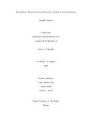
of a known sill in Effingham Inlet on the west coast of Vancouver Island, Canada (Figure 1).

Monk, S. A.
Effingham Inlet connects to Barkley Sound, and then the northeast Pacific, on the west Coast of
Vancouver Island, Canada. A number of sills divide this 17 km long fjord into three basins. The
upper basin has been the focus of several studies, because it is regularly anoxic. This study
reports on observations made on variations in surface circulation that occurs between the two
upper most basins of the inlet. This is where a sill 45 m deep separates a 200 meter deep basin
from a channel 100 meters deep.
There is a long history in using drifters to observe currents; the Challenger Expedition
first used drifters to monitor ocean circulation over 130 years ago (Thompson, 1877).
Historically drifters’ positions were found by radio direction finding triangulation giving sparse
data points (Davis, 1985). The use of GPS means that the location of the drifter can be
determined at shorter time intervals. Improvements have been made to these initial designs, with
the availability of affordable ways to log drifter position, through Global Positioning System
(GPS). These modifications in design allow more accurate measurements to be made in

Page 7 of 22
Lagrangian study of fjordic surface circulation
recording spatial and temporal information, which characterize the individual tracks.
Methods
Drifter Design
Deployment site south of
sill in basin
Deployment site north of sill
in channel
Figure 1. Location of Effingham Inlet, British Columbia Canada.
Triangles depicting the drifter deployment locations. a) Effingham
Inlet, with depth contours note the 45 m sill between the lower and
upper basin, after Kumar and Patterson (2002). b) Geographic
location of Effingham Inlet on Vancouver Island, after Kumar and
Patterson (2002). c) Bathymetric Profile, showing the sill that
separates the deployment sites, after Hay et al (2003).
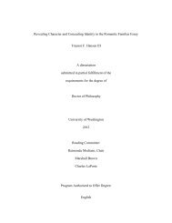
Two different drifter designs were used to record variation in the surface and near surface
circulation patterns in Effingham Inlet. The circulation of the surface 1 m of water was recorded

Monk, S. A.
Figure 2. Surface Drifter. a) Deployment of Surface Drifter in Effingham Inlet, photograph
credit to Kathy Newell. b) Schematic of a Davis Drifter, from NOAA (2006)
using a modified Davis style drifter (Figure 2). This drifter design was first proposed by Davis
(1983, 1985) and was used by the US Coastal Dynamics Experiment (CODE). The design has
been widely used and forms the basis for many drifter designs (Austin and Atkinson, 2004). The
original design allows the drifter to follow the surface movements, without picking up movement
due to wind and waves. The version used in this experiment consisted of a PVC frame; with
fabric sails arranged in a cross, with buoyancy provided by four floats, one on the end of each
arm. The main modification from previous designs to the frame was the inclusion of triangular
sections of fabric between the top arms, to prevent the drifter from tipping.
Technological advances such as GPS have improved the ability of drifters to record more
detailed information about their tracks. The surface drifter utilized two different GPS units, one

Page 9 of 22
Lagrangian study of fjordic surface circulation
to log location and the second to aid in recovery. The position data was logged by the GARMIN
eTrex® H, this sensitive unit is accurate to less than 10 m (root mean square) and waterproof.
The position was logged every 30 seconds, which was then downloaded using the MapSource
software after drifter recovery. The second GPS system was a GARMIN Astro®, this consists of
two GPS units, which can communicate their locations relative to each other using radio waves
within a 8 km radius, line of sight. Obtaining the range and bearing to the drifter was
instrumental in securing a fast drifter recovery, minimizing lost data.
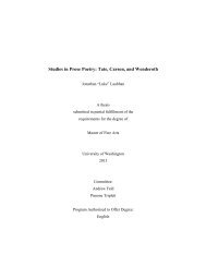
The second type of drifter used to track water at 5 meters below the surface was a
modified “Holey Sock” design (Figure 3). These types of drifters have been used in many
experiments, not limited to the Surface Velocity Program (SVP) and World Ocean Circulation
Experiment (Lumpkin and Pazos, 2007). The basic design is a small floating cylindrical surface
unit, which houses the GPS unit and is small enough to not be significantly affected by the wind.
This is tethered to a fabric tube 3 m below. The tube is 3 m long, 0.5 m in diameter, with holes
with of diameter of 0.2 m, cut at regular intervals. The tube acts as a drogue and the holes act to
catch the water and make sure the drogue follows the water. Work by Niller et al (1995) for the
SVP calculated that in order not to be slipping through the water the drogue needs to have a drag
area ratio greater than 40, and this arrangement, with a tunnel 3 m long and with a diameter of
0.5 m, has a drag area ratio of 39.7. This means it is acceptable to assume the drifter is following
the water motion. This near surface drifter also used the GARMIN eTrex® H to log its position,
however the transmitting GPS unit is not feasible on this design due to the smaller surface unit.

Monk, S. A.
Figure 3. Near Surface Drogue. When deployed only the surface unit remains above water,
and the tube extends to give the “Holey Sock”. a) Labeled photograph of a drifter taken
during deployment, photograph credit to Kathy Newell. Once in the water the tube sinks and
extends. b) An annotated schematic of the drogue after Lumpkin and Pazos (2007).
Drifter Deployment Strategy
The investigation was carried out on the 20 th and 21 st of March 2010, in the Effingham
Inlet. The R.V. Barkley Star from the Bamfield Marine Sciences Centre was the platform from
which operations were mounted. Each day, at slightly different stages in the tidal cycle, two pairs
of drifters were deployed either side of a sill 7 km from the mouth, where Effingham Inlet meets
the Barkley Sound. Each pair consisted of one surface drifter and one near-surface drifter. The
temporal scale for each deployment was between 4 and 6 hours.
Results

Page 11 of 22
Lagrangian study of fjordic surface circulation
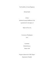
On the first day of this experiment all of the surface drifters and near surface drogues
moved toward the north (Figure 4). The surface drifters traveled further than the near surface
Holey Sock drogues. However the near surface drogue deployed south of the sill failed to deploy
properly, failing to extend to its proper depth and as a result acted somewhat like a surface
drifter.
a) b)
Figure 4. Map showing the paths taken by the surface drifters and near surface drogue,
overlaid on an image of Effingham Inlet. a) Paths for the first deployment. b) Paths for the
second deployment.
The fastest speeds were achieved by the surface drifter deployed north of the sill. This
drifter reached maximum speeds of close 0.55 m/s, over twice as fast as the speeds recorded by
the surface drifter deployed to the south of the sill. This maximum speed was reached in the
afternoon after low speeds in the morning (figure 5a). The near surface drogue north of the sill
traveled slowly for the first hour and half, with a slight increase in speed for the second half of

Monk, S. A.
the deployment (figure 5d). The variation in the speed around 0.03 m/s for this drogue is likely to
be due to the drifter speed being close to the accuracy limit for the GPS.
Surface Drifter Speed
(m/s)
Near Surface Drifter Speed
(m/s)
e)
Depth (m)
a) 3a)
b) 3b)
0.25
0.6
Drifter Speed
0.20
0.15
0.10
0.05
0.00
c)
3c)
0.14 Drogue Speed
0.12
0.10
0.08
0.06
0.04
0.02
0.00
09:00 10:00 11:00 12:00 13:00 14:00
Time
50
100
200
For the 3 days preceding the deployments, no precipitation was measured at the Bamfield
weather station. In the nine hours before the first deployment the prevailing winds were low; less
Drifter Speed m/s
0.5
0.4
0.3
0.2
0.1
0.0
3d)
Drifter Speed
Drogue Speed
Outer Basin Inner Basin
11:00 12:00 13:00 14:00
Time
Figure 5 Drifter Speeds recorded on the 20 March 2010, speeds recorded very 30 seconds
binned into 10 minute bins. The surface drifters displayed in the top line as crosses,
representing their shape, and the deeper drogues shown as circles, representing the Holey
Socks. a) Surface drifter speeds south of the sill in the outer basin. b) Surface drifter speeds
north of the sill, in the inner basin note this moved much faster than other drifter.. c) 5 m
drogue speed south of the sill, this drogue failed to sink. d) 5 m drogue speeds north the sill.
e) Bathymetric profile, arranged to illustrate the differences between the deployment
locations, after Hay et al (2003).
d)

than 3 km/hour and consistently from
southeast (Figure 6). During the first half of
the deployment the winds remained low. In
the afternoon the wind picked up to 10
km/hr and was consistently from the south.
Low tide for Effingham was at 10:10 am
(figure 7).
Figure 7. Tide predictions for the
deployments (indicated by arrows)
On the second day the surface
Wind Speed (km/hour)
Wind Direction (degrees from north)
Page 13 of 22
Lagrangian study of fjordic surface circulation
Wind Speed Recorded at Bamfield Marine Science Centr
20th March 2010
0
00:00 04:00 08:00 12:00 16:00 20:00 00:00
drifters recorded a different route (Figure 4b). Initially the two surface drifters both moved south
a)
b)
14
12
10
8
6
4
2
Time
Wind Direction Recorded at Bamfield Marine Science Centre
20th March 2010
300
250
200
150
100
50
00:00 04:00 08:00 12:00 16:00 20:00 00:00
Time
Figure 6. Wind data recorded by the Bamfield weather
station on the 20 th March 2010. Data recorded every
minute binned into 30 min bins. a) Wind speed in
km/hour. b) Wind Direction, shown in degrees from
north. Grey shaded area indicates deployment times.

Monk, S. A.
toward the mouth of Effingham. Then mid way through the deployment the drifter in the south
basin changed direction and returned north up the channel. The deeper drogues followed similar
paths to the previous day; both continuously moved to the north.
The surface speeds this day showed little variation between the two locations with both
surface drifters reaching average speeds of around 0.15 m/s (Figure 8a and 8b). The speeds of the
surface drifters were at least twice as fast as the speed of the deeper drogues, which averaged
around 0.05 m/s. The speeds of the deeper drogues varied between the two deployment locations
over the duration of the investigation. The near surface drogue south the sill showed little
variation in speed over the day remaining around 0.05 m/s, but the near surface drogue north of

the sill showed a trend of slightly increased speeds after 11:00.
Surface Drifter Speed
(m/s)
Near Surface Drifter Speed
(m/s)
e)
Depth (m)
5a) a) b) 5b)
0.30
0.25
0.20
0.15
0.10
0.05
0.00
c) 5c)
0.10
0.08
0.06
0.04
0.02
Drogue Speed
Drifter Speed
0.00
09:00 11:00 Time13:00
15:00
50
100
200
Page 15 of 22
Lagrangian study of fjordic surface circulation
Drifter Speed
In the 16 hours prior to the second deployment, 30 mm of precipitation was measured at
Bamfield. The prevailing wind was much more varied than the conditions of the previous day, its
d) 5d)
Drogue Speed
Outer Basin Inner Basin
09:00 11:00 Time 13:00 15:0
Figure 8 Drifter Speeds recorded on the 21 March 2010, speeds recorded very 30 seconds
binned into 10-minute bins. The surface drifters displayed in the top line as crosses,
representing their shape, and the deeper drogues shown as circles, representing the Holey
Socks. a) Surface drifter speeds below the sill in the outer basin. b) Surface drifter speeds
above the sill, in the inner basin. c) 5 m drogue speed below the sill, this drogue failed to
sink. d) 5 m drogue speeds above the sill. e) Bathymetric profile, arranged to illustrate the
differences between the deployment locations, after Hay et al (2003).

Monk, S. A.
speed varied by 8 km/hour and its direction varied by 100 degrees (Figure 9). During the
deployment, wind speeds were lower than
the previous day, never going above 8
km/hour. The wind direction was
predominantly from the south and was less
variable than the preceding winds, only
varying by 40 degrees. The low tide was at
11:00, then rising as the deployment
progressed.
A measure of “sinuosity”, or path
complexity, was derived for the path of each
drifter. This metric is often used to describe
the shape complexity of rivers, and is
calculated as the total path length by the
drifter and dividing it by the Euclidean
(straight line) distance traveled (Schumm,
1963). A non-complex path, or straight line,
would have a value of 1, while a complex
path would have a high value. The most
complex tracks were south of the sill (Table
1).
Wind Speed (km/hour)
Wind Direction (degrees from north)
a)
Wind Speed Recorded at Bamfield Marine Science Centre
21st March 2010
12
10
8
6
4
2
0
00:00 04:00 08:00 12:00
Time
16:00 20:00 00:00
b)
Wind Direction Recorded at Bamfield Marine Science Centre
21st March 2010
300
250
200
150
100
50
00:00 04:00 08:00 12:00
Time
16:00 20:00 00:00
Figure 9. Wind data recorded by the Bamfield weather
station on the 21 st March 2010. Data recorded every
minute binned into 30 min bins. a) Wind speed in
km/hour. b) Wind Direction, shown in degrees from
north. Grey shaded area indicates deployment times.

Discussion
Page 17 of 22
Lagrangian study of fjordic surface circulation
Table 1. Track complexity calculated by dividing path length by Euclidean length.
Date Location
20 March
2010
21 March
2010
Surface south of
the sill
Surface north of
the sill
Near surface
north of the sill
Surface south of
the sill
Near surface
south of the sill
Surface north of
the sill
Near surface
north of the sill
Total Path
Length (m)
The surface drifters followed different paths on each day. The tide had shifted little, so
was not the driving factor in controlling the motions. Prior to the first deployment there had been
no precipitation for three days, this would have lead to low terrestrial freshwater input. The
prevailing wind while low was from a constant direction for the nine hours before deployment.
As the river flow was low the prevailing winds were able to drive the surface motion to the
north. Prior to the second deployment 30 mm of rain fell in 16 hours at Bamfield. This
precipitation would increase the terrestrial inputs of fresh water. The prevailing winds were also
much more variable than the previous day, and unable to set up motions in the same way they
had the day before. The higher river flow was the dominant force on the surface motion on this
day, driving the surface flow to the south, towards the ocean.
Euclidean Length
(m)
Complexity
1580 1000 1.6
2205 2040 1.1
250 230 1.1
2840 680 4.2
750 480 1.6
1840 1750 1.1
800 640 1.2

Monk, S. A.
This finding is supported by previous studies which have demonstrated that when the
fresh water inputs are low the prevailing wind is the dominant force in controlling the surface
motions (Gade, 1963, Johannessen, 1968 and Svendsen and Thompson, 1978). Svendsen and
Thompson (1978) conducted research on a Norwegian Fjord and concluded that the surface
motion was setup by wind over a time scale of 10 hours. This is similar to the length of time the
prevailing winds were constant preceding the first deployment.
The near surface drogues moved in the same direction on both deployments, so were not
being controlled by the same driving force as the surface drifters. They traveled at similar
speeds, with small increases over the course of each deployment. The lowest speeds were
achieved at low tide, and increased as the tides flooded. A study in Alberni Inlet, a fjord 15 km
away that also connects to Barkley Sound, concluded that the deeper motions were the result of
the tide (Farmer and Osborn, 1976). This shows that it is likely that the 5 m drogues are
experiencing a tidal forcing. This would be confirmed by a longer deployment, covering an
entire tidal cycle.
The tracks in the basin south of the sill were the most complex and the tracks in the
channel to the south were consistently less complex. This shows that the drifters moved in a
simpler way in the channel. The basin geomorphology was wider and deep, while the channel
was confined by the sill at its mouth, steep walls and narrow width. This allowed the more
complex paths to be followed in the basin. The lower complexities in the channel are the result of
the flow being confined by the geomorphology. The fastest surface speeds were recorded in the
channel on the day when the wind was driving the flow north up Effingham Inlet. The wind was
forcing a large volume of water, north from the wide bay to narrow channel. The geomorphology
of the channel was then funneling this, which caused the speeds to increase. This may also offer

Page 19 of 22
Lagrangian study of fjordic surface circulation
one explanation for the observed increase in near surface speeds north of the sill seen on both
deployments, when there was little variation in the basin. The tide would be focused and the
speeds increased in the same way as the water being driven by the wind.
This study was limited to two consecutive days in spring. The deployments were of short
duration, insufficient to completely sample an entire tidal cycle. Despite these limitations the
results are in agreement with other studies focused on fjord estuaries.
Conclusions
The surface circulation patterns are influenced by many different factors. Prevailing
winds, fresh water inputs and tides combine to act as the major controlling processes in the
surface circulation of Effingham Inlet. There appears to be two separate systems at work to
control the circulation in the upper 1 m and the deeper 5 m layer. The surface layer is
predominantly influenced by the prevailing wind and fresh water input. When the fresh water
input is low the winds act as the dominant forcing. The opposite then holds true when the fresh
water input increases. The deeper layer is tidally forced and over this short term study showed
little response to the freshwater input. This finding is in line with previous results for fjords in
other areas. The local geomorphology of the basin also appears to be important in determining
the circulation patterns. Tracks are less complex in channels than those in basins, where the
water is confined. The geomorphology can funnel the circulation and produce more rapid speeds
under certain conditions.
In the future, conducting similar experiments over a longer time scale and during
different weather patterns would improve the reliability of these results. Another interesting

Monk, S. A.
experimental design should deploy the drifters and drogues in pairs to divergence in multiple
depth layers and specifically assess the spatial and temporal scales of these divergences.

References
Page 21 of 22
Lagrangian study of fjordic surface circulation
Austin, J. and S. Atkinson. 2004. The desgian and testing of small, low cost GPS tracked surface
drifters. Esturaies. 27: 1026-1029.
Bennett, M. 2001. The morphology, structural evolution and significance of push moraines. Earth
Science Reviews. 53:197-236.
Cannon, G. A. 1975. Observations of bottom-water flushing in a fjord like estuary. Estuarine and
Coastal Marine Science. 3:95-102.
Davis, R. E. 1983. Current-following drifters in CODE, Ref 83-4, pp. 74, Scripps Inst. Oceanogr., La
Jolla, Calif.
Davis, R. E. 1985. Drifter observations of coastal surface currents during CODE: the method and
descriptive view. J. Geophys. Res., 90: 4741-4755.
Farmer, D. M. and T. R. Osborn. 1976. The influence of wind on the surface layer of a stratified Inlet:
Part 1 Obersvations. Journal of Physical Oceanography. 6:931-941.
Gade, H. G. 1963. Some Hydrographic observations of the inner Oslofjord during 1959. Hvalradets Skr.,
46.
Hay, H. B., R. Pienitz and R. E. Thomson. 2003. Distribution of diatom surface sediment assemblages
within Effingham Inlet, a temperate fjord on the west coast of Vancouver Island (Canada).
Marine Micropalaeontology. 48: 291-320.
Hodgins, D. O. 1978. A time dependant two layer model of fjord circulation and its application to
Alberni Inlet, British Columbia. Estuarine and Coastal marine Science 8:361-378.
Johannessen, O. M. 1968. Some current measurements in the Droback Sound, the narrow entrance to the
Oslofjord. Hvalradets Skr., 48.
Kumar, A. and T. R. Patterson. 2002. Dinoflagellate cyst assemblages from Effingham Inlet, Vancouver
Island, British Columbia, Canada. Palaeography, Palaeoclimatology, Palaeoecology. 180: 187-
206.
Leonov, D. and M. Kawase. 2009. Sill Dynamics and fjord deep water renewal: Idealized modeling
study. Continental Shelf Research. 29: 22-233.
Lumpkin, R. and M. Pazos. 2007. Measuring surface currents with Surface Velocity Program drifters:
the instrument, its data, and some recent results, p. 39-67. In A. Griffa, A. D. Kirwan, JR., A. J.
Mariano, T. M. Ozgokmen, and T. Rossby [eds.], Lagrangian analysis and prediction of coastal
and ocean dynamics. Cambridge University Press.

Monk, S. A.
Niiler, P. P., A. Sybrandy, K. Bi, P. Poulain and D. Bitterman. 1995. Measurements of the waterfollowing
capability of Holey-sock and TRISTAR drifters. Deep-Sea Res., 42: 1951-1964.
Schumm, S. A. 1963. Sinuosity of alluvial rivers on the Great Plains. Geological society of America.
74:1089-1100.
Stigebrandt, A. 1980. Some aspects of tidal interactions with fjord constrictions. Estuarine and Coastal
Marine Science. 11:151-166.
Svendsen, H. and R. O. R. Y. Thompson. 1978. Wind-driven circulation in a fjord. Journal of Physical
Oceanography. 8:703-712.
Syvitski, J. P. M. and J. Shaw. 1995. Sedimentology and geomorphology of fjords, p113-168. In G. M.
E. Perillo [ed.], Geormorphology and sedimentology of estuaries. Elseview.
Thompson, C. W. 1877. A Preliminary Account of the General Results of the Voyage of the HMS
Challenger. MacMillan, London.